Global Navigation Satellite System (GNSS) radio occultation climatologies mapped by machine learning and Bayesian interpolation

Global Navigation Satellite System (GNSS) radio occultation (RO) is a space-based remote sensing technique that measures the bending angle of GNSS signals as they traverse the Earth's atmosphere. Profiles of the microwave index of refraction can be calculated from the bending angles. High accuracy, long-term stability, and all-weather capability make this technique attractive to meteorologists and climatologists. Meteorologists routinely assimilate RO observations into numerical weather models. RO-based climatologies, however, are complicated to construct as their sampling densities are highly non-uniform and too sparse to resolve synoptic variability in the atmosphere.

In this work, we investigate the potential of machine learning (ML) to construct RO climatologies and compare the results of an ML construction with Bayesian interpolation (BI), a state-of-the-art method to generate maps of RO products. We develop a feed-forward neural network applied to Constellation Observing System for Meteorology, Ionosphere, and Climate-2 (COSMIC-2) RO observations and evaluate the performance of BI and ML by analysis of residuals when applied to test data. We also simulate data taken from the atmospheric analyses produced by the European Centre for Medium-Range Weather Forecasts (ECMWF) in order to test the resolving power of BI and ML. Atmospheric temperature, pressure, and water vapor are used to calculate microwave refractivity at 2, 3, 5, 8, 15, and 20 km in geopotential height, with each level representing a different dynamical regime of the atmosphere. The simulated data are the values of microwave refractivity produced by ECMWF at the geolocations of the COSMIC-2 RO constellation, which fall equatorward of 46° in latitude. The maps of refractivity produced using the neural networks better match the true maps produced by ECMWF than maps using BI. The best results are obtained when fusing BI and ML, specifically when applying ML to the post-fit residuals of BI. At the six iso-heights, we obtain post-fit residuals of 10.9, 9.1, 5.3, 1.6, 0.6, and 0.3 N units for BI and 8.7, 6.6, 3.6, 1.1, 0.3, and 0.2 N units for the fused BI&ML. These results are independent of season.

The BI&ML method improves the effective horizontal resolution of the posterior longitude–latitude refractivity maps. By projecting the original and the inferred maps at 2 km in iso-height onto spherical harmonics, we find that the BI-only technique can resolve refractivity in the horizontal up to spherical harmonic degree 8, while BI&ML can resolve maps of refractivity using the same input data up to spherical harmonic degree 14.

1 Introduction

Earth radio occultation (RO) sounds temperature and water vapor in the Earth's atmosphere by measuring the refraction-induced frequency shifting of the signals of the Global Navigation Satellite System (GNSS) as received by satellites in low-Earth orbit (LEO). The RO remote sensing technique has been thoroughly described in several previous works, e.g., Kursinski et al. (1997, 2000), Melbourne (2004), and Mannucci et al. (2021). As an active limb-sounding technique, it provides highly accurate information on temperature and water vapor with 100 m vertical resolution from the surface to the stratopause but with non-homogeneous, non-uniform, and sparse horizontal sampling. In order to convert the soundings to a gridded dataset, special algorithms must be devised to map the data in the horizontal. The horizontal sampling is non-homogeneous because the orbital configurations of the multiple RO spacecraft have not been coordinated and because of the orbits of the satellites in the GNSS constellations. Consequently, local time coverage is generally incomplete and meridional coverage is at times neglected. Because of orbital dynamics, gaps in the RO sampling pattern occur at specific, well-defined latitudes (Leroy et al., 2012). The horizontal sampling distribution is also sparse because the density of RO soundings has never been high enough to sample every cell of synoptic variability in the atmospheric system, where a cell is approximately described by a span of several hours and the atmospheric Rossby radius of deformation. Mapping RO data requires statistical methods that weight the RO observations that do exist in a manner that minimizes the errors incurred by under-sampling the atmosphere without inducing biases.

Two approaches have been developed to construct gridded RO climatologies. The first approach is referred to as sampling-error removal. It uses the forecasts of a numerical weather prediction (NWP) model to estimate the sampling error associated with synoptic variability and incomplete coverage of the diurnal cycle. In this approach, the forecasts of an NWP system are interpolated to the locations and times of RO soundings, binned and averaged into longitude–latitude boxes just as the actual RO soundings are, and compared to the gridded predictions to estimate the bias associated with the binning and averaging. This estimate of the bias is then subtracted from the actual binned-and-averaged RO data (Foelsche et al., 2008, 2011). The other approach is Bayesian interpolation (BI) on a sphere, wherein linear combinations of spherical harmonics as basis functions are fit to RO data without overfitting the data (MacKay, 1992; Leroy et al., 2012). There have been many other applications of BI, and it has been evaluated in detailed analyses as a method for constructing climatologies of RO data (Leroy et al., 2012, 2021).

In this work, we use machine learning (ML) to produce RO climatologies. The ability of ML to learn from large amounts of data has been shown in many research subjects and applications (Hassanien, 2018). Neural networks are well-suited to the problem of estimating most probable values related to generalized inputs, which is the same problem that affects gridding RO data in the horizontal. Unlike the sampling-error-removal approach, neither BI nor ML requires external datasets to form objective gridded climatologies of RO data. At its core BI superposes spherical harmonics, while ML is based on more general mathematical functions. Spherical harmonics are orthogonal on a sphere but do not necessarily represent structures of atmospheric variability well. The more generalized interpolators of ML should prove to be more capable of resolving complex fine-scale horizontal structure.

ML has already been used successfully on ground-based GNSS observations. For decades, parameters estimated from GNSS data (station coordinates, troposphere, ionosphere, etc.) have been routinely quantified at permanent geodetic stations. In addition, the size and resolution of GNSS networks have increased, following the requirements of meteorologists, geodesists, and geophysicists. Thus, a large amount of data has been produced, which has naturally generated interest in applying ML algorithms to these datasets. Kiani Shahvandi et al. (2022), Gou et al. (2023), and Natras et al. (2022) applied ML to improve the prediction of important parameters needed in GNSS applications, such as polar motion prediction, ultra-rapid orbits, and the ionosphere, while Crocetti et al. (2021) used ML to detect discontinuities in time series of GNSS station coordinates.

ML algorithms have been successfully used to model meteorological products derived from GNSS observations in the past. For instance, in Miotti et al. (2020) and Shehaj (2023), ML was applied to tropospheric observations from ground-based GNSS to model them based on meteorological parameters. Miotti et al. (2020) showed that ML could model the implicit relation between zenith total delays (ZTDs) estimated at ground-based GNSS stations and meteorological parameters measured at permanent meteorological stations. While Miotti et al. (2020) demonstrated the applicability of ML to map time series of GNSS tropospheric observations, in Shehaj et al. (2023) ML and least-squares collocation were combined to produce high-resolution ZTD fields.

In other work, ML has been applied to tropospheric delays estimated at GNSS ground-based stations for the prediction of Alpine foehn (Aichinger-Rosenberger et al., 2022) or to spatially map zenith wet delay at a global scale, as in Crocetti et al. (2024). Kitpracha et al. (2019) used long short-term memory (LSTM) and a combination of singular spectrum analysis and Copula to predict zenith delays based on previous meteorological and delay series; errors of 2 and 1 cm were reported for a prediction of 24 h. In Shamshiri et al. (2019), an ML Gaussian process to model tropospheric delays in InSAR based on zenith delays was used, reporting an improvement of 81 % on the tropospheric corrections of the interferograms. In Zhang and Yao (2021), ML was applied to fuse precipitable water vapor from GNSS, MODIS (Moderate-Resolution Imaging Spectroradiometer), and the numerical weather model ERA5. In Shi et al. (2023), a method to efficiently generate zenith delays for the massive GNSS CORS (continuously operating reference station) network utilizing ML was developed. Gou and Soja (2024) use ML to enhance the global resolution of total water storage anomalies, with a spatial resolution of 0.5°.

While in previous work ML was successfully deployed to map time series of GNSS ground-based atmospheric observations, in this work we apply ML for spatial and temporal mapping of GNSS RO measurements. We exploit the large number of RO measurements (thousands daily) and the ability of ML to learn patterns from large datasets.

We develop a neural network for interpolating RO data in 6 h cycles in order to create gridded climatologies and compare the results to maps generated using BI. We can only compare our ML approach to BI since it provides a posteriori uncertainty but the sampling-error-removal method does not. We also estimate performance with simulation-mapping experiments using the output of an NWP system as a “nature run”. In doing so, we treat the gridded model output as truth against which we compare the output of the various mapping methods we consider. The outcomes are estimates of the uncertainty and the performance of each mapping approach.

Several studies have also applied ML to model residuals of observations, computed as the difference between a model not based on ML and target observations. The most typical cases originate from using physical models for prediction and from training an ML model to predict the residual part. For example, Wang et al. (2017) showed that ML could be used to model the difference between a superior model that is computationally expensive and a simple model to predict the component of the total stress tensor in a fluid. Similarly, Gou et al. (2023) applied several ML and deep learning (DL) algorithms to model the differences between GNSS final orbit products and ultra-rapid-orbit products. Therefore, their ML model could help overcome the limitations of simplified physics-based orbit propagators by training on residuals. Kiani Shahvandi et al. (2023) used a method based on neural networks (NNs) named ResLearner to calibrate the rapid Earth orientation parameters (EOPs) with respect to the final EOPs in a residual manner. In this work, we also propose a loosely coupled combination of ML and BI, in which we first apply BI to the observations and then train the ML model on the BI residuals.

The second section of this paper describes the data that we use. The third section describes the BI and ML mapping algorithms. The fourth section contains the analysis of a numerical experiment that probes the performance of BI and ML. Finally, the fifth section presents a summary and discussion of the results and future work.

2 Data

2.1 COSMIC-2/FORMOSAT-7

The Constellation Observing System for Meteorology, Ionosphere, and Climate-2, COSMIC-2/FORMOSAT-7 mission is operated by the National Oceanic and Atmospheric Administration (NOAA), the US Air Force (USAF), Taiwan's National Space Organization (NSPO), the University Consortium for Atmospheric Research (UCAR), and other partners (UCAR, 2022a; Ho et al., 2020; Schreiner et al., 2020). At present, COSMIC-2 obtains RO soundings from the transmitters of the US Global Positioning System (GPS) and the Russian Globalnaya Navigazionnaya Sputnikovaya Sistema (GLONASS), providing approximately 6000 high-performance profiles of refractivity daily and covering the Earth from latitudes of 46° S to 46° N . We use analyzed refractivity sourced from wetPf2 files from the data portal of the COSMIC project office of UCAR. The wetPf2 NetCDF files contain geometric altitude above mean sea level, geopotential height above mean sea level, longitude, latitude, temperature, pressure, water vapor partial pressure, specific humidity, relative humidity, dry temperature, dry pressure, and refractivity for each level of the atmospheric sounding. In this work, we use geometric altitude above mean sea level, longitude, latitude, and refractivity.

We interpolate the COSMIC-2 refractivity profiles to isohypsic surfaces at 2, 3, 5, 8, 15, and 20 km above mean sea level. These levels show a wide variety of morphologies in spatiotemporal structures because of the very different physical phenomena prevalent at each level.

• 2 km (Fig. 1a). At this height, we notice small-scale structures related to boundary layer clouds and water vapor.

• 3 km (Fig. 1b). At this height, there is still an important contribution from the water vapor to refractivity, but it is just outside the planetary boundary layer. We expect the retrieved refractivity to have higher quality than at 2 km since Abel inversion for refractivity encounters its largest errors within the boundary layer, usually associated with super-refraction and tracking difficulties.

• 5 km (Fig. 1c) and 8 km (Fig. 1d). Synoptic, jet stream, and frontal variability dominate the dynamics of refractivity, with a smaller contribution of water vapor than in the boundary layer.

• 15 km (Fig. 1e). Mixing across the subtropical front by baroclinic eddies in the stratospheric “middle world” dominates. In the midlatitudes, we are in the stratosphere, while in the tropics we are in the troposphere. This is depicted in Fig. 1, where a clear distinction – almost a step function – in refractivity is experienced between the tropics and midlatitudes.

• 20 km (Fig. 1f). Larger structures of the atmosphere relate to planetary-scale waves in the lower stratosphere.

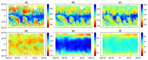
Figure 1 COSMIC-2 RO refractivity distributions on six isohypsic surfaces for the period 1–10 January 2020, illustrating the very different spatiotemporal morphologies at each level. The refractivity at 2, 3, 5, 8, 15, and 20 km is visualized in panels (a), (b), (c), (d), (e), and (f), respectively. The color bar units are N units (ppm), i.e., refractivity units; the x axis is longitude; and the y axis is latitude.

We utilize COSMIC-2 data representing 10 d time series of the four seasons. The measurements spanning 1–10 January 2020 represent boreal winter (40 000 profiles), 1–10 April 2020 represent boreal spring (40 000 profiles), 3–12 July 2020 represent summer (30 000 profiles), and 1–10 October 2020 represent fall (30 000 profiles). The criterion to select these time spans was continuity, meaning that we simply chose the first 10 continuous days with RO profiles for each season of 2020.

2.2 ECMWF operational forecasts

In order to create a nature run on which to test ML mapping schemes, we interpolated the forecasts of the operational weather prediction system of the European Centre for Medium-range Weather Forecasts (ECMWF) to the times and locations of COSMIC-2 RO soundings, spanning 1–10 January 2020. Specifically, we used the output of ECMWF Integrated Forecast System (IFS) cycles 46r1 and 47r1; see ECMWF (2023). Using forecast fields rather than analysis fields, complications that arise from assimilating COSMIC-2 RO data into ECMWF operational analyses are avoided. Forecasts are always physically consistent three-dimensional fields of the atmosphere, in as much as the physics is defined by the prognostic model. NWP analyses, however, are physically inconsistent because the data that constrain the atmospheric state perturb the state in isolated regions away from physical consistency. We obtained NetCDF files of pressure, temperature, water vapor, and geopotential fields with a horizontal resolution of 0.5°. We used 12 h forecast fields, which are published hourly.

We computed refractivity profiles (and geometric altitude above mean sea level) at the times and locations of COSMIC-2 RO soundings at the grid points in operational forecasts. Refractivity N is related to the microwave index of refraction n and atmospheric properties (Rueger, 2002):

$$\begin{array}{}\text{(1)}& \begin{array}{rl}N& =\left(n-\mathrm{1}\right)\times {\mathrm{10}}^{\mathrm{6}}=\left(\mathrm{77.6890}\mathrm{K}{\mathrm{hPa}}^{-\mathrm{1}}\right){\displaystyle \frac{\left(p-p_w\right)}{T}}\\ & +\left(\mathrm{71.2952}\mathrm{K}{\mathrm{hPa}}^{-\mathrm{1}}\right){\displaystyle \frac{p_w}{T}}+\left(\mathrm{375463}{\mathrm{K}}^{\mathrm{2}}{\mathrm{hPa}}^{-\mathrm{1}}\right){\displaystyle \frac{p_w}{T^{\mathrm{2}}}},\end{array}\end{array}$$

where p, p_w, and T are the atmospheric pressure, the partial pressure of water vapor, and temperature, respectively. This formulation of refractivity accounts for fixed and induced dipoles of nitrogen, oxygen, carbon dioxide, and water vapor but neglects compressibility effects. The refractivity of surface air generally falls in the interval of 320–360 N units, about 10 % of which is due to water vapor, with larger values at lower latitudes where more water vapor is present. When interpolating the model to the times and locations of COSMIC-2 RO soundings, we took the model refractivity profile in the cell nearest to the RO sounding and interpolated linearly in altitude, the vertical dimension.

Finally, we interpolated the refractivity for each profile to the six chosen altitudes listed in Sect. 2.1. Using ECMWF data with resolutions of 0.5° in latitude and longitude and 1 h in time, we locate the closest forecast geolocations and times from the COSMIC-2 RO data.

3 Methods

We introduce two RO mapping techniques in this section: Bayesian interpolation on a sphere and machine learning via neural networks.

3.1 Bayesian interpolation (BI)

Bayesian interpolation (BI) works by fitting irregularly gridded and noisy data using a superposition of basis functions without overfitting the data (MacKay, 1992). The input to the method is a set of scalar values with associated longitudes and latitudes and possibly even local (solar) times. The output is an inference of a two-dimensional field and its uncertainty as the coefficients of a spherical harmonic expansion and sines and cosines in the diurnal cycle, along with an associated uncertainty covariance matrix of those coefficients. Diagnostics of the process yield information on the effective degrees of freedom of the signal – and hence the horizontal resolution of the map – a single value describing the “measurement” error in every input value, and on the Bayesian evidence for the fit, otherwise known as the joint probability of the model and the data. While largely an objective method, it nevertheless does involve some tuning of the regularization matrix, the purpose of which is to prevent overfitting of the data. We use a regularization matrix that asymptotes to stable values of Bayesian evidence with increasingly large spherical harmonic expansions (Leroy et al., 2012). In doing so, we assure that output mappings are neither penalized nor rewarded for increasing numbers of basis functions beyond some nominal expansion.

BI is well-suited to map GNSS RO data because the sampling patterns are highly irregular, and synoptic variability acts as a source of noise (Leroy, 1997). On a sphere, the natural basis functions are spherical harmonics, and BI using spherical harmonics as basis functions has been explored in depth to generate level 3 climatologies (i.e., latitude–longitude gridded products) of GNSS RO data (Leroy et al., 2012, 2021). For this work, we use the same Python module developed by Leroy et al. (2012, 2021). We map RO observations in latitude and longitude and use the BI results to compare and combine them with ML. While BI on a sphere is intended for globally distributed non-uniformly sampled data, it also works well when the data are restricted geographically. In our application, COSMIC-2 RO sounding distributions are restricted to the tropics and to the oceans. An example of a BI map is shown in Fig. 5b.

3.2 Machine learning applied to RO

We use the classical artificial neural network algorithm multilayer perceptrons (MLPs) detailed in Haykin (2009). This algorithm is widely applied to large datasets. We apply a fully connected neural network, where the neurons of one layer are connected to all the neurons of the previous one. The first layer consists of the inputs and the last one of the target values. Each neuron is computed as follows (Haykin, 2009):

$$\begin{array}{}\text{(2)}& \mathrm{neuron}=f(\sum _{i=\mathrm{1}}^n\mathrm{neuron}\mathrm{\_}\mathrm{previous}\mathrm{\_}{\mathrm{layer}}_i\cdot w_i+b),\end{array}$$

where a weight w_i is computed for each neuron of the previous layer, and a bias b is added. The bias and weights are the parameters of the neural network.

The inputs and outputs have complex relations. The activation function f defines the nonlinearity. The most common activation function is the rectified linear unit function (ReLU); it suppresses neurons with negative values (Nwankpa et al., 2018):

$$\begin{array}{}\text{(3)}& f\left(x\right)=\max (\mathrm{0},x).\end{array}$$

The training process adapts all the network parameters so that the input/output relation will be accurate. The hidden layers are functions of the neurons in the previous layers. Thus, we relate the output and input layers as follows:

$$\begin{array}{}\text{(4)}& \mathrm{pred}=F\mathit{\{}{\mathrm{feature}}_{\mathrm{1}},\mathrm{\dots }{\mathrm{feature}}_n\mathit{\}},\end{array}$$

where feature_n represents the nth input variable. The prediction pred can be compared to the true value (label) directly. Therefore, a loss function can be calculated with the typical formulation for regression purposes, i.e., the mean-squared error (MSE):

$$\begin{array}{}\text{(5)}& \mathrm{MSE}={\displaystyle \frac{\mathrm{1}}{n}}\sum _{i=\mathrm{1}}^n{\left({\mathrm{pred}}_i-{\mathrm{label}}_i\right)}^{\mathrm{2}}.\end{array}$$

The parameters of the neural network, i.e., the weights and biases, describe the loss function. We aim to minimize the loss function, and thus the set of parameters that best satisfies this condition is defined by the network. The local minimum of the loss function is searched for using stochastic gradient descent.

Another step is the standardization of the data before the training process. This is applied to avoid numerical issues. The mean (μ) and standard deviation (σ) of the training dataset are used to standardize each feature x separately as follows:

$$\begin{array}{}\text{(6)}& x{}^{\prime }=(x-\mathit{\mu })/\mathit{\sigma }.\end{array}$$

Thus, the feature variables are scaled to a standard deviation of 1 and centered around zero. This mainly affects the search for local minima using gradient descent. Introducing features with very different values (and value variations) might result in a steep gradient descent, leading to a solution that is not optimal. For a deeper look into neural networks, we refer the readers to Hastie et al. (2009) and Stanford (2023).

Note that MLP is not necessarily the best algorithm for our research question, but our ultimate goal in this research is not to find the most appropriate one. Our objective is to demonstrate that ML can be used to map RO data and that it provides comparable (or better) results compared to state-of-the-art methods.

3.3 Machine learning applied to Bayesian interpolation residuals

We also develop a method where we combine BI with ML, named BI&ML. In this case, we train on residuals of BI. The procedure is as follows.

• We apply BI to the training dataset. We compute the spherical harmonic coefficients with the same 80 % of the data that are used for training in ML.

• We compute residuals of the BI applied to the training dataset.

• We train the neural network using the BI post-fit residuals (of the training dataset) as a target and using longitude, latitude, and time as inputs. The tuning of the hyperparameters is done as explained in Sect. 4.

• We compute error statistics by comparing BI&ML refractivities with the test dataset.

4 Analysis

Here we apply mapping to real and simulated COSMIC-2 data. Our application is an interpolation problem, with the goal of mapping RO data in longitude, latitude, and time.

In the first step of the analysis, we compare the post-fit residuals of the BI, ML, and BI&ML approaches based on actual COSMIC-2 RO data. In the second step, we evaluate the performance of the BI and BI&ML approaches using the atmospheric analyses of the ECMWF operational products as a nature run. Initially, we compute the (gridded) residuals for simulated ECMWF refractivities at COSMIC RO locations, and then we evaluate the effective horizontal resolution of these two approaches.

To fit the BI and ML models, we use 10 d of COSMIC-2 data and ECMWF forecasts. A longer time span of data does not affect the results of ML; however, BI is more sensitive to the length of data. Indeed, BI is only able to estimate the best spatial fit to an entire 10 d dataset. The atmospheric state evolves over each 10 d period, and thus BI can only estimate a time-average state with less horizontal structure. A period of 10 d is a compromise to have enough data to properly train the ML models and at the same time produce BI climatologies with little averaging over time. Unlike BI, in our tests, ML can produce climatologies with a very high temporal resolution.

In the first subsection (Sect. 4.1), we give the results for hyperparameter tuning for ML and BI&ML. In the second subsection (Sect. 4.2), we compare the relative performance of all three approaches described in Sect. 3 at different heights in the atmosphere. In the third subsection (Sect. 4.3), we analyze the consequences for our ability to resolve spatial and temporal variability in fields that can be measured by RO.

4.1 Tuning hyperparameters

One important step when working with neural networks is tuning the hyperparameters, which define the architecture or how the training process is performed. When defining the hyperparameters that determine the architecture of the network, such as the number of layers and number of neurons per layer, one option is to add layers until the error can no longer be reduced. A larger number of parameters allows for complexity in mappings; thus, adding more layers can improve the complexity of fitting. A larger number of parameters, however, can also lead to overfitting. If necessary, regularization methods (such as dropout) can be used to prevent overfitting.

As is customary in ML, we randomly split the nature dataset into three segments: 72 % of the data for training, 8 % for validation, and 20 % for testing. We point out that the training, validation, and testing datasets do not overlap. By random choice, we mean that we do not split them according to a specific parameter (such as time, geolocation, or refractivity values). Since we neither assume different accuracies of the training and testing datasets nor teach the network any specific random behavior of the test dataset, we expect the accuracy of the model fitted to the training dataset to be similar for the testing dataset. Therefore, a very good fit in the training dataset does not bias the testing. Indeed, we get similar post-fit residuals for both datasets; this is considered a successful evaluation of the model resulting from the training dataset.

In addition, in one exercise, for each block of 10 d of data, we use the first 8 d for training and the last 2 d for testing. This makes our task a prediction problem and not an interpolation problem. We evaluate the quality of this approach by intentionally overfitting the training data, resulting in overly large errors when applied to the testing data as expected. We can explain this result by the fact that there are different structures in the refractivity field for the testing dataset that have not been seen by the network during the training. This exercise demonstrates overfitting in prediction, proving our ML architecture ill-suited for prediction but not for interpolation.

4.1.1 Hyperparameter tuning for the ML approach

After tuning, we settled upon a final architecture consisting of five hidden layers, with the first having 512 neurons and the next four having 128 neurons. It is not unusual for neural networks to have different numbers of neurons in each layer leading to similar error statistics. The input layer consists of three variables, namely longitude, latitude, and time, and the output layer produces microwave refractivity.

We tuned variables that determine how the training is done, where the choice of learning rate, the batch size, and the number of epochs impacted the results the most. The final values that we chose are 0.0001, 100, and 30 000, respectively. Note that we designed different neural networks to train refractivities at the different altitudes (shown in Sect. 2.1). Although we used the same final hyperparameter values for all networks, in some cases a different choice provided similar (but not better) statistics. For instance, at 20 km in altitude for learning rate, batch size, and number of epochs, using 0.0001, 250, and 30000 or 0.001, 250, and 15 000 led to similar results. An example of hyperparameter tuning is shown in Fig. 2, where the best results are shown in more distinct colors. We also trained the number of layers, the optimizer, and the weight decay. However, we did not notice any significant differences when using different optimizers or weight decay.

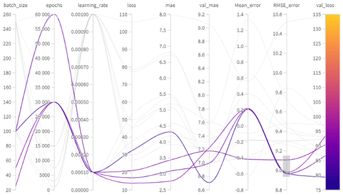
Figure 2 Hyperparameter tuning in ML, visualized in weights and biases (https://wandb.ai/site, last access: 26 September 2023). The first three columns contain the values tried during the tuning process for three main hyperparameters (batch size, epochs, and learning rate). The next columns contain statistics that we can use to evaluate the performance of candidate combinations of tuned hyperparameters. The fourth column (loss) represents the loss function (mean squared error function) of the training dataset. The fifth (mae) and sixth (val_mae) columns represent the mean absolute error in the training and validation dataset. The seventh (mean_error) and eighth (RMSE_error) columns represent the mean error and the root-mean-squared error in the testing dataset. The final column (val_loss) defines the loss function for the validation dataset. The validation loss is the metric chosen to tune the hyperparameters, and the color bar represents its results. Following the curves, we can define the best set of hyperparameters. The validation dataset represents a randomly chosen 10 % of the training dataset, utilized to tune the hyperparameters. The statistics of the validation dataset can be easily computed and were therefore chosen as a metric to select the hyperparameters. The highlighted curves show the best results on the testing dataset in terms of root-mean-squared error for the different tunings, arbitrarily chosen for this visualization.

4.1.2 Hyperparameter tuning for the BI&ML approach

Once more, we trained different neural networks for six refractivity altitudes. The architecture of the MLP is the same as that shown in Sect. 4.1.1, consisting of five hidden layers, with the first having 512 neurons and the next four having 128 neurons. The input layer has three variables, namely longitude, latitude, and time, and the output layer delivers BI residuals of microwave refractivity. The learning rate is again 0.0001 for all networks. The tuned batch size and number of epochs are 25 and 2000, respectively, for the networks of 2, 3, and 5 km in altitude; 50 and 1000 for the network of 8 km in altitude; and 100 and 4000 for the networks of 15 and 20 km in altitude. Again, other possible hyperparameter choices could result in similar (but not better) results; for example, we could choose for the dataset at 5 km in altitude a learning rate of 0.001, batch size of 250, and number of epochs of 1000. Different tunings with similar results were especially encountered when training data at high altitudes. One reason is that the target value variations become very small, and it is possible to learn them with different values for learning rate, number of batch sizes, and/or number of epochs. Training BI residuals instead of total refractivity values leads to a faster training process. One explanation is that the network can learn more quickly when the targets have smaller variations.

4.2 Performance evaluation for real RO data

Using the BI and ML models obtained from the training dataset, we mapped the observations of the test dataset, which is 20 % of the data, and then we computed the residuals for the six chosen heights. Figure 3 displays the residuals for the three methods (BI, ML, and BI&ML), and Table 1 summarizes the statistics in terms of the standard deviation (SD) and mean relative error (MRE). The MRE represents the mean of the residuals scaled by the true values of the refractivity.

• As expected, the residuals are higher at lower altitudes for each method. This is logical since the refractivity values are higher and more spatially variable at lower altitudes (see Fig. 3), and the Abel inversion results in larger errors at lower altitudes. Therefore, the noise in the observations is also higher at lower altitudes.

• The spatial distribution of the larger residuals is different for the different heights. For instance, at the lower heights, we can find most of the high residuals of BI in the tropics, while at 15 km they are located in the mid latitudes. This is the case since the mapping methods miss the high jumps in the refractivity values due to approximation of RO data and low resolution of RO data. At 2 and 3 km, these jumps occur mainly in the tropics, related to higher water vapor, and in the mountainous areas, where the distribution of water vapor can highly vary on the different sides. At 15 km, the mapping functions fail to approximate the large refractivity jumps between the troposphere (in the tropics) and the stratosphere (in the midlatitudes).

• We notice that when we apply ML, the refractivity jumps at 15 km from the tropics to the midlatitudes are captured well.

• From Fig. 3, it might be difficult to understand the benefit of applying ML to RO residuals after applying BI. However, from the statistics in Table 1, we notice an improvement of about 5 %–10 % compared to ML-only. One advantage of applying ML to RO residuals is in terms of interpretation of the dataset used to fit the ML model. For instance, at 15 km we expect ML to learn from the distinct pattern of BI residuals (where the large residuals occur in the midlatitudes) and to further improve these results. In addition, as mentioned in Sect. 4.1.2, ML applied to RO residuals is much more efficient in terms of the time needed to train the ML models. In our experiments, the time to train the neural network is proportional to the number of epochs and the batch size. For example, in the case of two different models, if we use the same batch size, a doubling of the number of epochs doubles the training time. Similarly, if we consider the same number of epochs, a batch size two times smaller doubles the training time. Other hyperparameters can also affect the training time, such as the type of optimizer, the number of neurons, and the learning rate (a smaller learning rate requires a larger number of epochs); however, these parameters are the same for the different neural networks that we use.

The overall best configuration, which we will focus on in Sect. 4.3, is the ML approach applied to the residuals of BI.

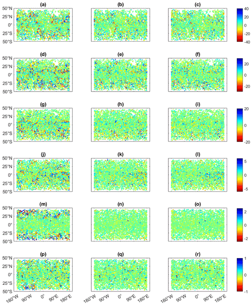
Figure 3 Residuals for the test dataset of the refractivity interpolated with BI, ML, and BI&ML for the six pre-defined isohypsic surfaces for COSMIC-2 RO data. The units are N units (refractivity units), the x axis is longitude, and the y axis is latitude. Panels (a), (d), (g), (j), (m), and (p) display BI residuals at 2, 3, 5, 8, 15, and 20 km, respectively. Panels (b), (e), (h), (k), (n), and (q) display ML residuals at 2, 3, 5, 8, 15, and 20 km, respectively. Panels (c), (f), (i), (l), (o), and (r) display BI&ML residuals at 2, 3, 5, 8, 15, and 20 km, respectively.

Figure 4 displays the increment of BI&ML over the ML-only and BI-only approaches at 3 km in altitude. The increment of BI&ML over BI-only has large values mainly in the geolocations, where we can visualize large jumps in refractivity within few degrees (latitude and/or longitude). The increment of BI&ML over ML-only has a more random distribution of large values. These values happen mainly in locations where the residuals of ML and/or BI&ML (see Fig. 3) have a larger density. By training on BI residuals, we anticipated better results since a part of the refractivity behavior is already removed; however, since the spatial resolution of RO data is not very high, BI does not always capture the spatial refractivity changes very well (especially when sudden refractivity changes happen). This may lead to higher relative changes between the residuals compared to the total values; thus, the trained values in the ML model have larger variations. In addition, since BI is a screen over the 10 d, the mapped refractivity for similar locations can be more accurate for some epochs of the 10 d time span. Since we do not label the noise of each input feature differently when we train the ML models, ML will consider all residuals as having the same weight, which will impact its mapping accuracy. However, from the statistics in Table 1, we can see that ML applied to BI residuals results in better generalization for the entire time span and surface. Indeed, it removes most of the complex atmospheric dynamics and simplifies the entire variation in the target variables.

We expect ML-only to be the best approach when we deal with specific atmospheric structures happening on a specific day during the 10 d time span. For instance, in the case of atmospheric rivers, BI would fail to capture these structures since it will find the best fit of the 10 d dataset. Therefore, it will result in large variations in the residuals, making them more complex to train on than total refractivities.

Results in different seasons at 2 km

We also validated the results obtained for winter 2020 with the other seasons of the same year. Table 2 summarizes the results of the three mapping methods for each season at 2 km in altitude. At 2 km in altitude, RO observations are noisier compared to the other altitudes, because of larger absolute values and larger errors resulting from the Abel inversion. In addition, their uncertainty and variation are higher since it is at this height that the largest percentage of water vapor is located. For all the seasons, the best performance is achieved for the combined solution, resulting in a further improvement compared to BI-only and ML-only. Note again that each of the neural networks was tuned separately to achieve the best possible solution.

Table 1 Statistics of BI, ML, and BI&ML mapping methods at six predefined heights for winter 2020 for COSMIC-2 RO data. The bold-formatted values represent the best statistics amongst the three cases: ML, BI, and BI&ML.

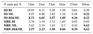
Table 2 Statistics of BI, ML, and BI&ML mapping methods for the four different seasons at 2 km in height for COSMIC-2 RO data. The bold-formatted values represent the best statistics amongst the three cases: ML, BI, and BI&ML.

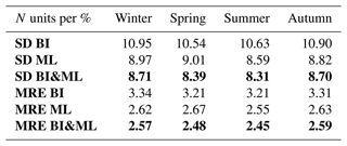
Note that the results displayed in this section (Tables 1 and 2) are a result of one single trained network and not of an ensemble of networks. To further validate our results, we performed additional experiments for the refractivity at 2 km in iso-height, where we trained multiple (10) models for ML and BI&ML. For our architecture, similar results were achieved to the results of the ensemble of the models, with a standard deviation ∼ 0.2 N units worse. In addition, for the ensemble of models, we noticed further improvements (mainly on the standard deviation) when we added more hidden layers. On an ensemble of 10 trained models, a ∼ 0.3 N units improvement can be achieved when using 10 hidden layers, compared to 5 layers for the ML model. However, this further increases the training time, which is especially important for the ML method given that we use a total of 30 000 epochs. A higher number of layers is more suitable for BI&ML, where the number of epochs is much smaller.

We point out that the scope of this study is to present ML as an alternative method to grid RO observations. The results obtained herein indicate better performance compared to BI. Considering our results and the additional tests with multiple models, BI&ML brings additional (small) improvement compared to ML methods, with an obvious advantage in terms of a much shorter time needed to train the model. For future work related to continuous long-term RO-gridded products, an ensemble of models will be trained to also provide the uncertainty related to the models.

4.3 Post-fit residuals of BI, ML, and BI&ML mapping techniques applied to ECMWF

We compare the post-fit residuals of the BI approach, the ML approach, and the combined BI&ML by applying each to the 10 d nature run of ECMWF forecast products. We perform a similar evaluation for ECMWF as we did for the COSMIC-2 data, where we split the data into training and test samples and apply the three methods. We obtain, in terms of standard deviation and mean relative error, 12.4 N units and 3.8 % for BI, 11.1 N units and 3.3 % for ML, and 10.7 N units and 3.1 % for BI&ML. We confirm that mapping ECMWF (forecast) refractivities (interpolated at COSMIC-2 geolocations) results in performance similar to the mapping of COSMIC-2 refractivities.

4.3.1 Structural improvement: spatial and temporal resolution compared to ECMWF maps

We mapped the ECMWF-based simulated refractivities with BI and BI&ML to the same locations as the ECMWF grid points. An example of the maps (at 2 km in height) is displayed in Fig. 5, where the original ECMWF refractivity field for one epoch is displayed as well. We can see the very high resolution of the original ECMWF map compared to the interpolated ones. The BI-mapped field is the screen over the 10 d dataset, while that of the BI&ML represents the interpolation at only one epoch. We produced maps with a resolution of 3 h. The ML-based maps are produced with much higher temporal resolution compared to those with BI (a resolution of 3 d reported in previous works; Leroy et al. (2021). In addition, Fig. 6 displays the difference between the original ECMWF and the mapped refractivity fields. There are several areas where the high differences between the ECMWF and BI-based maps are further smoothed by applying ML to the BI residuals.

Figure 6 displays only 1 map of the total of 80 maps that we produced for the 10 d period. To compare the results for each epoch, Fig. 7 displays the statistics for every map as a function of time. There is an improvement in the intervals: [0.5; 2] N units and [0.5; 1] % in terms of standard deviation and the mean relative error, respectively.

Figure 4 The difference between BI&ML and ML-only(a) and the difference between BI&ML and BI-only (b) for COSMIC-2 RO data. The units are N units, refractivity units; the x axis is longitude; and the y axis is latitude.

Figure 5 ECMWF refractivity grid (a), BI-mapped refractivity grid (b), and BI&ML-mapped refractivity grid (c) for 2 January 2020 at 03:00 UTC. The units are N units, refractivity units; the x axis is longitude; and the y axis is latitude.

4.3.2 Effective horizontal resolution

After fitting the BI and BI&ML models, we can produce refractivity maps with a very high spatial resolution. However, the interpolated resolution is not the actual resolution that the methods can capture for the spatial behavior of the refractivity. To evaluate what level of information BI and BI&ML can produce in terms of horizontal resolution, we use the original and mapped fields to compute spherical harmonic spectral coefficients up to a very high order (such as 120). We visualize the power (and variance of the fit dataset compared to those of ECMWF) as a function of degree (or horizontal resolution).

Each of the datasets can be expressed as a spherical harmonic expansion (Muir and Tkalcic, 2015):

$$\begin{array}{}\text{(7)}& \mathit{\psi }\left(\mathit{\theta },\mathit{\lambda }\right)={\sum }_{l=\mathrm{0}}^{l_{\max }}{\sum }_{m=-l}^{m=l}{Y}_m^l\left(\mathit{\theta },\mathit{\lambda }\right)c_{l,m},\end{array}$$

where $Y_m^l\left(\mathit{\theta },\mathit{\lambda }\right)=N_{l,m}{P}_{l,m}\left(\sin \mathit{\theta }\right)e^{im\mathit{\lambda }}$ is the spherical harmonic of degree l and order m, and the c_l,m are complex spherical harmonics spectral coefficients. We can compute the spherical harmonics spectral coefficients by inverting Eq. (7):

$$\begin{array}{}\text{(8)}& c_{l,m}={\sum }_{j=\mathrm{1}}^{n_g}\left\{{\displaystyle \frac{\mathrm{1}}{\mathrm{2}\mathit{\pi }}}\underset{\mathrm{0}}{\overset{\mathrm{2}\mathit{\pi }}{\int }}\mathit{\psi }\left({\mathit{\theta }}_j,\mathit{\lambda }\right)e^{-im\mathit{\lambda }}d\mathit{\lambda }\right\}{P}_{l,m}\left(\sin {\mathit{\theta }}_j\right)g_j,\end{array}$$

which is computed over a defined Gaussian grid for $j=\mathrm{1}:n_g$ over latitude θ, with Gaussian weights g_j. We can compute the power at each degree as in Muir and Tkalcic (2015):

$$\begin{array}{}\text{(9)}& P\left(l\right)={\sum }_{m=\mathrm{0}}^l{\left|c_{l,m}\right|}^{\mathrm{2}}.\end{array}$$

In addition, we can compute the normalized power $P\mathit{\_}\mathrm{norm}\left(l\right)=P\left(l\right)/\mathrm{Hor}\mathrm{\_}\mathrm{res}\left(l\right)$, where the horizontal resolution is given as a function of the Earth's radius R_E, $\mathrm{Hor}\mathrm{\_}\mathrm{res}\left(l\right)=R_{\mathrm{E}}\sqrt{\mathrm{4}\mathit{\pi }}/(l+\mathrm{1})$.

We also evaluate the explained variance, defined as

$$\begin{array}{}\text{(10)}& \mathrm{Explained}\mathrm{\_}\mathrm{variance}\left(l\right)=\mathrm{1}-{\displaystyle \frac{\mathrm{Var}\left(l\mathrm{|}\mathrm{Fit}-\mathrm{ECMWF}\right)}{\mathrm{Var}\left(l\mathrm{|}\mathrm{ECMWF}\right)}}.\end{array}$$

Considering d_m=1 for m=0 and d_m=2 otherwise, the two variances can be computed as follows:

$$\begin{array}{}\text{(11)}& \begin{array}{rl}\mathrm{Var}& \left(l\mathrm{|}\mathrm{Fit}-\mathrm{ECMWF}\right)=\sum _{m=\mathrm{0}}^l{d}_m\left|c_{l,m}\left(\mathrm{BI}\mathrm{or}\mathrm{BI}\mathit{\&}\mathrm{ML}\right)\right.\\ & {\left.-c_{l,m}\left(\mathrm{ECMWF}\right)\right|}^{\mathrm{2}},\end{array}\end{array}$$

$$\begin{array}{}\text{(12)}& \mathrm{Var}\left(l\mathrm{|}\mathrm{ECMWF}\right)=\sum _{m=\mathrm{0}}^l{d}_m{\left|c_{l,m}\left(\mathrm{ECMWF}\right)\right|}^{\mathrm{2}}.\end{array}$$

To avoid non-orthogonality of spherical harmonics on non-global grids, we must consider observations covering the entire sphere. We randomly select values from the 10 d of the ECMWF forecast data grid, at latitudes that are not covered by the observations, i.e., outside the [−46°, 46°] latitude interval. The only condition we apply is to have the same spatial density as that in the latitude interval [−46°, 46°]. An example of the refractivity field (at 2 km) for 10 d in winter 2020 is shown in Fig. 8. This refractivity field is used to fit the BI and BI&ML models and therefore map the refractivity on the original ECMWF grid.

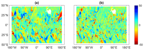
Figure 6 The difference between the ECMWF refractivity field and the refractivity fields mapped with BI for 2 January 2020 at 03:00 UTC (a). The difference between the ECMWF refractivity field and the refractivity fields mapped BI&ML for 2 January 2020 at 03:00 UTC (b). The units are N units, refractivity units; the x axis is longitude; and the y axis is latitude.

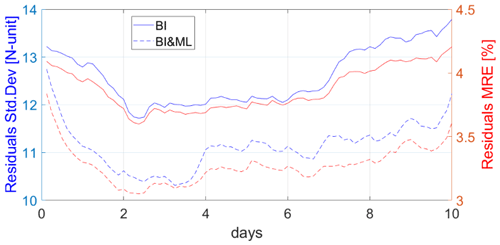
Figure 7 Standard deviation (left y axis) and mean relative error (right y axis) of the difference between the ECMWF refractivity field and those mapped with BI and BI& ML for all epochs.

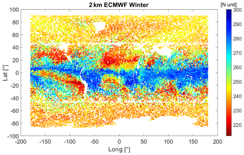
Figure 8 The ECMWF forecast refractivity field for 10 d in winter 2020 at a 2 km isohypsic surface. To compute spherical harmonics, we simulated refractivity at all latitudes. Between 46° S and 46° N, the refractivity is interpolated at the same times and locations as for the COSMIC-2 field. Below 46° S and above 46° N, we randomly chose refractivity values from the ECMWF data, with the criteria to keep the same density as that of COSMIC-2 between latitudes of 46° S and 46° N .

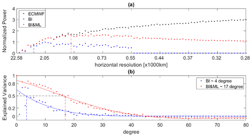
After fitting the BI and BI&ML models, we produce gridded N fields (similar to Fig. 5), which are used to compute the spherical harmonics spectral coefficients (Eq. 8). Figures 9 and 10 display the normalized power and the explained variance for two of the heights evaluated, 2 and 8 km. The power and explained variance displayed here are the average over the entire dataset of 80 maps in 10 d. From the power plots, we notice that the BI&ML curve (red dots) follows the ECMWF curve at a higher spherical harmonics degree (and thus horizontal resolution). We can also see that after 40 degrees the power of BI is zero. This is expected since the degree we chose for the BI was 40 as well.

We evaluate the explained variance at a value of 0.5, which represents the value where the power captured from the mapping methods is half of the original ECMWF power. We use this value as the metric to define the horizontal resolution of each method. From the explained variance plots in Figs. 9 and 10, we can see that BI can capture horizontal structures up to degree 8 (∼ 2500 km) at 2 km in height and up to degree 4 (∼ 4500 km) at 8 km in height. BI&ML can produce maps with a horizontal resolution of degree 14 (∼ 1500 km) at 2 km in height and of degree 16 (∼ 1250 km) at 8 km in height. These results represent the average over the entire set of 80 maps. For both heights and the majority of the maps produced, applying ML to BI residuals improves the spatial resolution by greater than a factor of 2 compared to the BI-only approach.

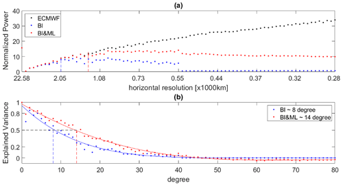
Figure 9 (a) Average (over time) normalized power for ECMWF, BI, and BI&ML, at 2 km in height. (b) Average (over time) explained variance for BI and BI&ML at 2 km in height.

Figure 10 (a) Average (over time) normalized power for ECMWF, BI, and BI&ML at 8 km in height. (b) Average (over time) explained variance for BI and BI&ML at 8 km in height.

5 Discussion and conclusions

In this work, we investigated ML as an alternative approach to mapping GNSS RO observations and compared it to BI, an approach used for many years to map GNSS RO data. In addition, we developed a combined solution where we map the residuals of BI using ML, referred to as BI&ML.

Starting with 10 d of COSMIC-2 GNSS RO profiles in boreal winter 2020, we mapped microwave refractivity at six predefined heights: (a) 2 km, where we notice small structures related to boundary layer clouds and water vapor; (b) 3 km, where there is still a large amount of water vapor; (c) 5 km, related to synoptic disturbances, pressure fields, storms, and precipitation; (d) 8 km, similar to 5 km but with smaller refractivity; (e) 15 km, where the eddy mixing in the stratospheric middle world occurs; and (f) 20 km, related to larger atmospheric structures from planetary waves in the lower stratosphere.

We used 80 % of the COSMIC-2 data to train/fit the BI, ML, and BI&ML models and evaluated the performance on the remaining 20 %. The ML-only solution results in better performance than the BI-only solution. Applying ML to the residuals of BI results in the best performance and a larger improvement compared to the state-of-the-art BI method. The posterior uncertainties for BI&ML are 8.7, 6.6, 3.6, 1.1, 0.3, and 0.2 N units, and the mean relative errors for BI&ML are 2.57 %, 2.23 %, 1.5 %, 0.66 %, 0.36 %, and 0.62 % for the six altitudes, respectively. The reduction in residuals for the ML-only and BI&ML at 15 km compared to BI-only are clearly visible (Fig. 6), where the refractivity values change significantly between the tropics (in the troposphere layer) and the midlatitudes (in the stratosphere layer). In addition, we fit the BI, ML, and BI&ML mapping approaches to 10 d of COSMIC-2 data for boreal spring, summer, and autumn 2020. We performed this evaluation at 2 km in iso-height, and we confirmed that the results obtained for the winter scenario apply to the other seasons as well.

We used NWP forecasts from ECMWF with a 0.5° latitude/longitude resolution to interpolate ECMWF refractivities to the geolocations and times of the COSMIC-2 data for 10 d for boreal winter 2020. We applied BI-only and BI&ML to map the simulated data at the ECMWF grid points, which we used as a nature run, and then performed a closed-loop validation. The map produced by BI&ML shows smaller residuals with respect to the nature ECMWF map than the BI-only map. In addition, the temporal resolution of the BI&ML maps is much higher than that of the BI-only maps. We produced BI&ML-based maps every 3 h (higher resolution is also possible), while BI-only needs at least 3 d of observations to produce a map. We investigated the spatial resolution of each method by spherical harmonic expansion, comparing the spectral coefficients of the BI-only and the BI&ML maps to the spectral coefficients of the nature ECMWF maps. After evaluating the explained variance of the coefficients, we concluded that BI-only can model refractivity variations up to spherical harmonic degree 8 and BI&ML up to spherical harmonic degree 14 at 2 km in iso-height. At 8 km in height, the improvement is more notable, with BI-only resolving only up to spherical harmonic degree 4, while BI&ML resolves up to spherical harmonic degree 17.

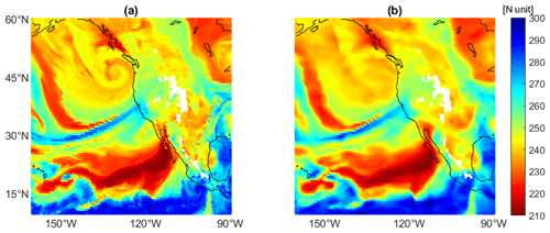
Figure 11 An example of refractivity at 2 km in altitude for 24 October 2021 at 16:00 UTC, similar to Shehaj (2023). (a) The ECMWF reference field. (b) The field mapped using ML (for the 60-satellite constellation).

We set out to investigate whether ML can offer an alternative to existing methods to map GNSS RO data, providing a so-called level 3 product. Existing methods include BI, which fits data using spatial basis functions without over-fitting data, and sampling-error-removal methods, in which synoptic variability noise is estimated by subsampling the forecasts of a numerical weather prediction system to the times and locations of RO soundings, computing the sampling error, and subtracting that sampling error from binned RO data. We compared ML methods to BI and found improved performance, and then we compared a combined BI&ML method and found a very substantial improvement in the performance over BI. We are unable to compare to sampling-error-removal approaches because they support no error estimation. All indications point toward the combined BI&ML approach as the best method for producing level 3 climatologies of RO data in the future, with strong performance even at timescales of 3 h at heights ranging from the planetary boundary layer up to the lower stratosphere and for all seasons.

When approaching specific atmospheric structures, the current spatial and temporal density of RO observations leads to a need for better coverage. Shehaj (2023) shows an example of using RO observations to detect atmospheric rivers (AR). ARs are long and narrow bands in the atmosphere that transport water vapor in regions beyond the tropics. Panel (a) in Fig. 11 shows an AR that occurred in October 2021, visualized as a blue stream using ECMWF refractivity at 2 km in altitude. In panel (b) in Fig. 11, ML was applied to simulated RO using the ECMWF 12 h forecast, assuming a 60-satellite LEO constellation tracking four GNSS constellations to generate a 2 km refractivity field. For the example in Fig. 11, we can see that with the ML-mapped field, we can resolve the AR structure. The ML field also depicts the dry patch located in the tropics. We also notice structures that are more difficult to resolve, such as the cyclone close to British Columbia and the high-refractivity patch close to Hawaii.

We point out that in Shehaj (2023) similar experiments were performed for this AR scenario using observations of the COSMIC-2 constellation; the number of RO observations is much smaller compared to the simulated example shown here. After applying the ML model to grid the COSMIC-2 refractivity (at 2 km in height), we cannot properly observe the spatial and temporal evolution of the AR structure.

The example in Fig. 11 shows the need for higher spatial and temporal density of RO observations and the benefit of using ML as a method to further enhance the resolution of the observations. In future studies, we will further explore the feasibility of GNSS RO for detection and monitoring of ARs.