A new technique to retrieve aerosol vertical profiles using micropulse lidar and ground-based aerosol measurements

Accurately characterizing the vertical distribution of aerosols and their cloud-forming properties is crucial for understanding aerosol-cloud interactions and their impact on climate. This study presents a novel technique for retrieving vertical profiles of aerosols, cloud condensation nuclei (CCN), and ice nucleating particles (INP) by combining micropulse lidar, radiosonde, and ground-based aerosol measurements. Herein, the technique is applied to data collected by our team at Texas A&M University during the Tracking Aerosol Convection Interactions ExpeRiment (TRACER) campaign. Ground-based aerosol size distribution and CCN counter data are used to estimate the value of the aerosol hygroscopicity parameter, κ. The derived κ, together with Mie scattering theory and the relative humidity profile from the radiosonde, is used to estimate aerosol size growth and the associated increase in backscatter at each altitude. We then correct the lidar backscatter to dry conditions to produce the dry aerosol backscatter coefficient profile. The dry aerosol backscatter coefficient profile is linearly scaled to collocated surface measurements of aerosols, CCN, and INP to produce corresponding vertical profiles. Combining lidar backscatter profiles with aerosol and cloud nucleation measurements leads to a more realistic representation of vertical distributions of aerosol properties. The method could be readily applied to lidar measurements in future field campaigns.

1 Introduction

The interaction between aerosols and clouds introduces significant uncertainties in estimating aerosol indirect radiative forcing, a critical factor in predicting future climate scenarios (Seinfeld et al., 2016). Aerosols can facilitate the formation of cloud droplets and ice particles by acting as cloud condensation nuclei (CCN) and ice nucleating particles (INP), respectively. Consequently, changes in aerosol concentrations could influence many cloud properties and processes (Tao et al., 2012; Fan et al., 2016; Twohy et al., 2005). For example, increased CCN concentrations could result in smaller cloud droplet sizes, suppress local precipitation in warm-phase clouds, and extend cloud lifetimes (Twomey, 1977; Albrecht, 1989). Some convective cloud studies have suggested that an increased concentration of ultrafine aerosol particles (smaller than 50 nm) leads to enhanced condensational heating from additional water vapor condensation. Since this process invigorates the updraft intensity, it has been referred to as warm-phase invigoration (Fan et al., 2007; Fan et al., 2018; Lebo and Seinfeld, 2011). Other studies have focused on cold-phase invigoration of updrafts, a process in which cloud water freezes, releasing latent heat and subsequently increasing the buoyancy of air parcels (Andreae et al., 2004; Rosenfeld et al., 2008). At present, the extent and significance of aerosol-induced invigoration effects are under debate (Lebo, 2018; Igel and van den Heever, 2021; Varble et al., 2023). Addressing these uncertainties requires a deeper understanding of the microphysical processes involved (Jensen, 2023). One of the key gaps in our current understanding of aerosol-cloud interactions is the vertical distribution of aerosols, CCN, and INPs in the cloud environment.

The knowledge of the aerosol vertical distribution is important for assessing aerosol-cloud interactions (Rosenfeld et al., 2014; Lin et al., 2023). Modeling studies have shown evidence that the altitude of aerosols significantly influences their impact on cloud formation and deep convection (Marinescu et al., 2017; Lebo, 2014; Zhang et al., 2021). However, in most long-term field campaigns, aerosol, CCN, and INP measurements are only made at ground-based sampling stations (Schmale et al., 2018; Pöhlker et al., 2016; Perkins et al., 2022). By comparison, airborne in situ measurements, which provide observations of CCN and INP at the cloud level, are generally of shorter duration (Stith et al., 2009; Dadashazar et al., 2022; Raes et al., 2000). Thus, retrievals from ground-based lidar observations, which can operate continuously over extended periods to quantitatively assess vertical profiles of aerosol properties, represent a highly valuable method.

Lidars detect range-resolved properties of aerosols and cloud particles by emitting laser pulses and measuring the backscattered light. Lidar measurements can be used to retrieve bulk aerosol optical properties, including the aerosol backscatter coefficient, extinction coefficient, and depolarization ratio. These aerosol optical properties are influenced by various aerosol properties, including size distribution, shape, chemical composition, and mixing state (Brooks et al., 2004b; Titos et al., 2016; Yao et al., 2022). Although the same intrinsic particle properties govern microphysics, the relationship between the lidar observations and the concentration of cloud-forming aerosols is not straightforward. Most CCN are found within the Aitken (typically between 0.01 and 0.1 µm) and accumulation (typically between 0.1 and 1 µm) aerosol modes, but lidar observations at visible wavelengths are most sensitive to the accumulation and coarse (typically greater than 1 µm) mode (Shinozuka et al., 2015; Kapustin et al., 2006). In addition, aerosol hygroscopic growth due to increased humidity increases the aerosol backscatter coefficient without affecting the CCN concentration (Shinozuka et al., 2015; Liu and Li, 2014). As for INP, it has been shown that larger aerosols are more likely to be INP, particularly those with a diameter exceeding 500 nm (DeMott et al., 2010). Individual aerosols in this size range backscatter light effectively, but less than 1 in 10⁵ particles in the atmosphere can act as INPs (DeMott et al., 2010). Thus, INPs contribute little to the measured bulk aerosol optical signals. Consequently, it is necessary to employ assumptions or complementary aerosol measurements when estimating cloud-forming aerosol concentration from remote sensing measurements.

Studies have adopted different approaches when using lidar measurements to retrieve the CCN concentration vertical profile (Lv et al., 2018; Mamouri and Ansmann, 2016; Ansmann et al., 2021; Ghan et al., 2006; Ghan and Collins, 2004; Lenhardt et al., 2023). The first approach involves using multiwavelength lidar to retrieve aerosol concentrations by classifying them into different aerosol types (urban, biomass burning, and dust) and then using the prescribed hygroscopicity parameter of each aerosol type to estimate the CCN concentration (Lv et al., 2018). This approach requires an advanced multiwavelength lidar, such as the multiwavelength High Spectral Resolution Lidar (HSRL-2) or the multiwavelength Raman lidar (Müller et al., 2011; Müller et al., 2014). Another approach relies on an empirical relation between the aerosol extinction coefficient and aerosol concentrations derived from the Aerosol Robotic Network (AERONET) to convert backscatter into aerosol concentration profiles. A CCN parameterization scheme based on the empirical relation between aerosol and CCN concentration of each aerosol type is applied to the aerosol concentration profile to produce the CCN concentration profile (Mamouri and Ansmann, 2016; Ansmann et al., 2021). Each of these approaches strongly relies on assumed aerosol composition, shape, and refractive index used in the lidar retrieval and CCN parameterizations. Consequently, they may fail to capture the complex conditions of atmospheric aerosols, thus limiting the precision of CCN estimations.

The third approach to determining CCN concentration using lidar is to directly scale ground-based CCN concentration measurement with the lidar-measured extinction or backscatter profile, first proposed by Ghan and Collins (2004). This approach assumes that the aerosol composition and size distribution remain relatively constant with altitude. Ghan and Collins (2004) used the humidification factor (hereby referred to as the lidar hygroscopic growth correction factor), defined as the dependence of aerosol extinction or backscatter on relative humidity (RH), to convert the observed extinction and backscatter coefficients to their dry counterparts. Ghan and Collins (2004) found that CCN concentrations at smaller supersaturations correlate more strongly with dry backscatter and are less impacted by height variations in aerosol size distribution than at higher supersaturations. Ghan et al. (2006) later validated this approach, showing that the correlation between lidar-derived and in situ CCN is influenced by supersaturation, aerosol uniformity with height, and lidar retrieval accuracy. This method has been applied in a routine CCN profile data product based on a Raman lidar (Kulkarni et al., 2023). Following a similar approach, Lenhardt et al. (2023) compared in situ CCN and airborne HSRL-2 measurements in the southeast Atlantic. Their results show that CCN concentration at 0.3 % supersaturation in dry ambient conditions (where RH ≤ 50 %) strongly correlates with the HSRL-2 measured extinction and backscatter. Collectively, these studies demonstrate the strong potential of lidar observations for retrieving CCN profiles.

Compared to the lidar retrievals of CCN, fewer studies have focused on INP retrievals using lidar data. Studies have combined INP parameterization with lidar measurement to retrieve INP concentration profiles (Mamouri and Ansmann, 2016; Marinou et al., 2019; Ansmann et al., 2021). A number of INP parameterization schemes based on previous ice nucleation measurements are available in the literature for total global aerosols of unspecified composition (DeMott et al., 2010), dust (Ullrich et al., 2017; DeMott et al., 2015; Niemand et al., 2012; Steinke et al., 2015), soot aerosols (Ullrich et al., 2017), biological aerosols (Tobo et al., 2013), and organics (Wang and Knopf, 2011). Generalized aerosol type and composition assumptions must be made when using these INP parameterizations, which depend on past measurements from other locations or lab experiments. In contrast, lidar retrievals based on simultaneous ground-based INP measurements would provide a more realistic estimate of ice nucleation. We propose that, analogous to CCN profile retrieval, INP concentration measured at the surface can be linearly scaled by the dry backscatter coefficient profile derived from lidar measurements to create an estimate of the INP vertical profile.

Despite advancements in understanding aerosol–cloud interactions, significant uncertainties remain in accurately characterizing aerosol vertical distributions and their impact on cloud processes, requiring more comprehensive and vertically resolved measurements to fill these knowledge gaps. The Tracking Aerosol Convection Interactions ExpeRiment (TRACER) campaign focused on understanding aerosol-cloud/convection interaction in the Houston metropolitan area in the summer and fall of 2022 (Jensen, 2023). In this study, we use the micropulse lidar and ground-based aerosol measurements we collected during the TRACER campaign to develop a measurement-based approach to retrieve the aerosol, CCN, and INP vertical profiles. The ground-based aerosol measurements include aerosol size distribution, CCN, and INP measurements. By leveraging observations to minimize assumptions in the retrieval process, this approach is expected to produce realistic vertical profiles of aerosol, CCN, and INP concentrations.

2 Methodology

2.1 Overview of TRACER Field Campaign

The US Department of Energy (DOE) TRACER field campaign was conducted from October 2021 through September 2022 in the Houston metropolitan area, with an intensive observation period (IOP) from June 2022 to September 2022, as shown in Fig. 1. The DOE first Atmospheric Radiation Measurement (ARM) Mobile Facility (AMF1) was deployed at La Porte, Texas, throughout the campaign. During the IOP, whenever forecasts indicated a strong sea breeze and conditions favorable for isolated deep convection, the TAMU ROAM-V was deployed at Seawolf Park in Galveston, Texas, and at several inland sites (Rapp et al., 2024). An overview of the TAMU TRACER campaign payload, deployment strategy, and available measurements is provided by Rapp et al. (2024). Both AMF1 and ROAM-V collected similar ground-based aerosol measurements, radiosonde data, and ground-based lidar profiles, as summarized in Table 1. The lidar retrieval method described below was developed based on the ROAM-V instrumentation and was also applied to the observations at the AMF1 site during TRACER. By extension, this method could be used in other future campaigns with a similar instrumentation configuration. All ROAM-V measurements, including the offline ice-nucleation array work, were conducted by our Texas A&M group (see Thompson et al., 2025a, b for details), and Table 1 lists the corresponding DOE ARM data-archive entries for each instrument.

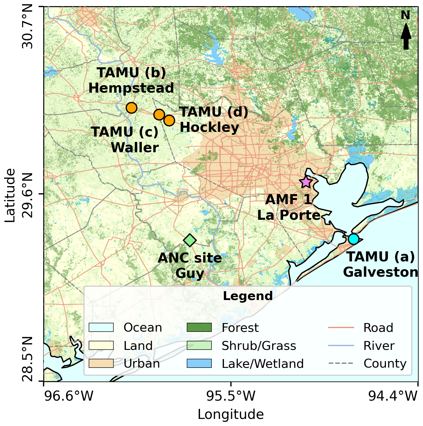
Figure 1 TRACER campaign sampling locations in the Houston, Texas, metropolitan area. The Texas A&M University sampling sites are marked with circles, the ARM AMF1 site is marked with a star, and the ARM ancillary site is marked with a diamond. This map was created using Natural Earth shapefiles, LandFire 2022 vegetation data, and USA detailed water bodies data (Rollins, 2009).

Table 1 A list of data and instruments used in this study.

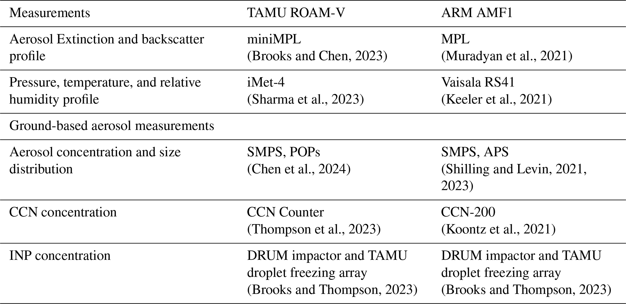
Figure 2 provides an overview of the retrieval routine for aerosol, CCN, and INP profiles using the TRACER campaign data. The routine is summarized here. First, we used lidar and radiosonde data to determine the vertical profile of the cloud-free aerosol backscatter coefficient. Next, the aerosol measurements from Scanning Mobility Particle Sizer (SMPS), Portable Optical Particle Spectrometer (POPS), and a cloud condensation nuclei (CCN) counter are used to estimate the lidar hygroscopic growth correction factor, f(RH), which is the ratio of aerosol backscatter coefficient at a given relative humidity (RH) to that at dry conditions. f(RH) and radiosonde-derived RH profile are then used to convert the aerosol backscatter coefficient profile to a dry aerosol backscatter coefficient profile. The resulting dry aerosol backscatter coefficient profile is used to linearly scale time-averaged surface aerosol concentration, CCN concentration, and INP concentration measurements to estimate their vertical distributions. Each profile is retrieved from data collected over a one to three hour period centered around radiosonde launch time.

Figure 2 Overview of the aerosol, CCN, and INP profile retrieval routine.

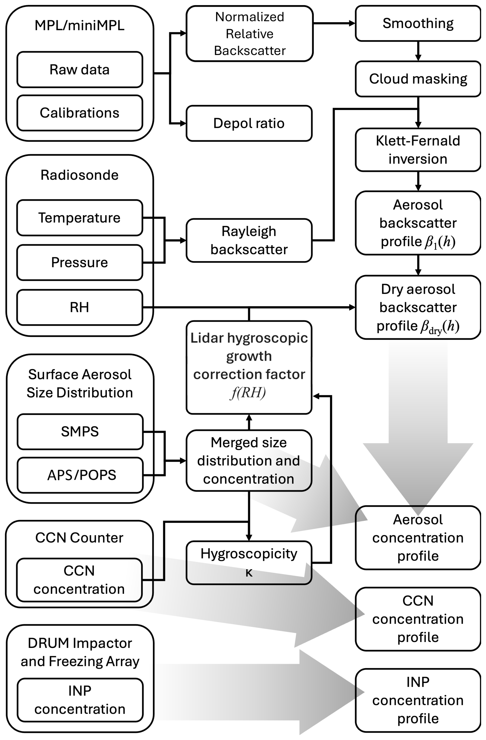
This method addresses the challenge that aerosol size distribution, composition, particle shape, and hygroscopic growth, all of which influence backscatter, are not directly measured by the micropulse lidar and must be inferred. By assuming that surface aerosol properties are representative of those of the whole column, the dry backscatter coefficient becomes approximately linearly proportional to aerosol volume concentration. We therefore could scale the time-averaged surface aerosol, CCN, and INP measurements with the lidar-derived dry backscatter profile to obtain their vertical distributions. Below, we discuss details of each step of the retrieval process with TAMU ROAM-V data collected on 28 August 2022 in Galveston, Texas, as an example.

2.2 Micropulse Lidar Measurement and Inversion of the Lidar Equation

The mini micropulse lidar (miniMPL, Droplet Measurement Technologies, Inc.) operates at 532 nm and measures backscatter and depolarization (Campbell et al., 2002; Flynn et al., 2007; Welton and Campbell, 2002). The miniMPL uses a vertical resolution of 15 m and a temporal resolution of 1 min in the TRACER campaign. The normalized relative backscatter (NRB), also known as the attenuated backscatter, is derived from the raw backscattered lidar signal after standard background, afterpulse, deadtime, and overlap corrections are performed. Details of the corrections are presented in the Supplement (Eqs. S1–S4). An example of an NRB time series collected by the miniMPL is shown in Fig. 3.

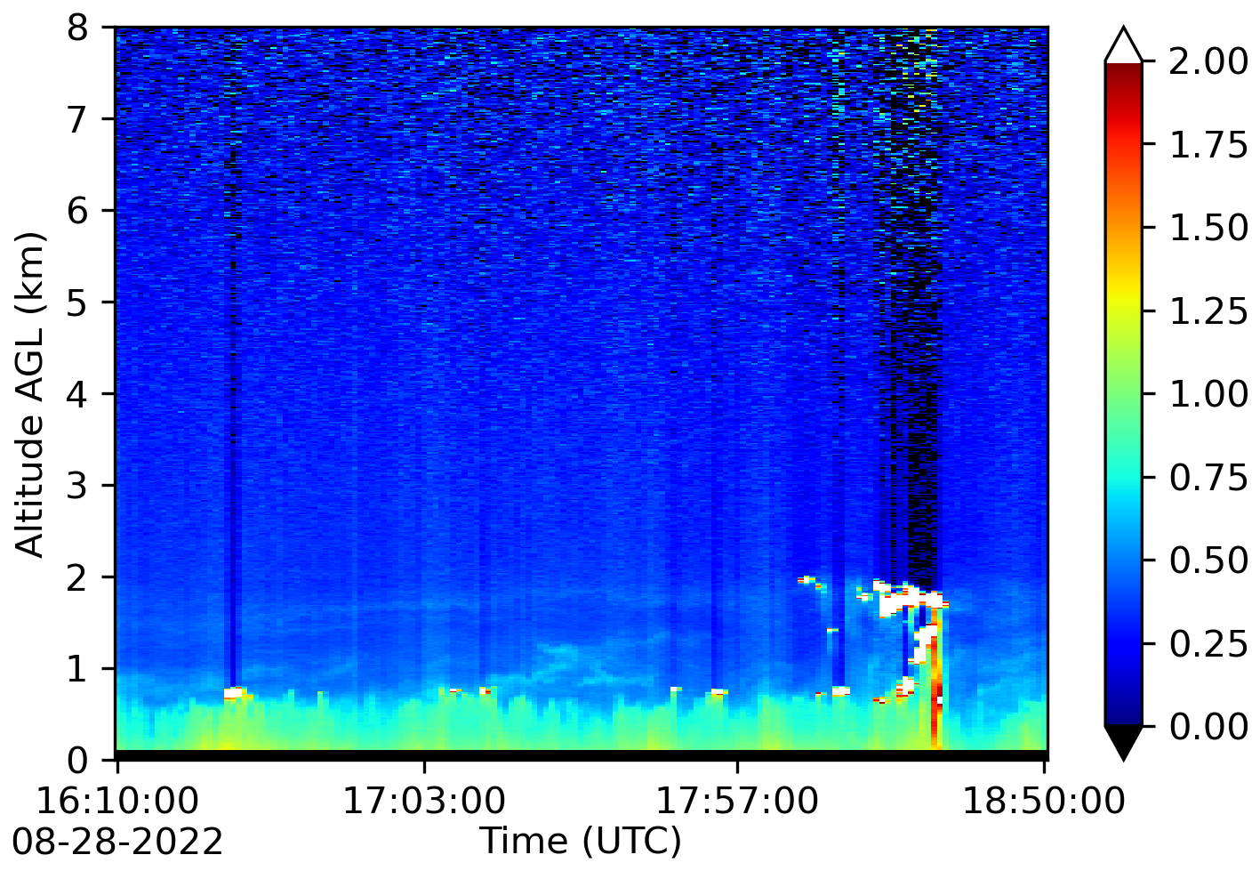
Figure 3 Normalized relative backscatter (NRB) time series collected on 28 August 2022, with miniMPL in Galveston, Texas.

NRB can be expressed as,

$$\begin{array}{}\text{(1)}& \mathrm{NRB}\left(R\right)=C\left[{\mathit{\beta }}_{\mathrm{1}}\right(R)+{\mathit{\beta }}_{\mathrm{2}}(R\left)\right]T_{\mathrm{1}}^{\mathrm{2}}\left(R\right)T_{\mathrm{2}}^{\mathrm{2}}\left(R\right)\end{array}$$

where R is the range, C is the lidar calibration constant, β₁ and β₂ represent the backscatter coefficient of aerosol and air molecules, respectively; T₁ and T₂ represent the transmittance of aerosol and air molecules, respectively. After correcting the raw lidar data to produce the NRB profile, data filtering and smoothing are applied to the NRB profile. First, a continuous wavelet transform based algorithm is used to create a cloud mask, filtering out periods of data with cloud signal peaks in the NRB profile that compromise the quality of aerosol retrieval (Du et al., 2006). Because the miniMPL collects measurements near the peak of the solar spectrum, observations can have a considerable amount of background noise during daytime measurements (Campbell et al., 2002). The NRB profiles of cloud-free columns, typically between 0.5 to 1.5 h before and after the radiosonde launch time (for a total of one to three hours), are time-averaged. The sensitivity of this aerosol profile retrieval method is shown in Sect. S4 of the Supplement. This averaged NRB profile is further normalized by the average NRB value of the lowest range bin. In addition, the NRB profile above 4.5 km is smoothed using the NeighBlock denoising algorithm based on the discrete wavelet transform to increase the stability of the retrieval process (Cai and Silverman, 2001). Similar wavelet transform techniques have been widely used in lidar applications for noise reduction and feature detection because the lidar signal exhibits a varying degree and frequency of noise at different ranges (Fang and Huang, 2004; Xie et al., 2017).

Next, a Fernald two-component lidar inversion method is performed. This is a classic method for solving the lidar equation and retrieving aerosol backscatter profiles from the attenuated backscatter (Fernald et al., 1972; Klett, 1981; Fernald, 1984; Sasano et al., 1985). The lidar ratio (S), defined as the ratio of aerosol extinction coefficient to aerosol backscatter coefficient, is assumed to be constant with respect to range (R). Following the Fernald method, the sum of aerosol (β₁(R)) and molecular backscatter coefficient (β₂(R)) is expressed as:

$$\begin{array}{}\text{(2)}& \begin{array}{rl}{\mathit{\beta }}_{\mathrm{1}}& \left(R\right)+{\mathit{\beta }}_{\mathrm{2}}\left(R\right)\\ & ={\displaystyle \frac{\mathrm{NRB}\left(R\right)\cdot e^{-\mathrm{2}(S_{\mathrm{1}}-S_{\mathrm{2}}){\int }_{R_{\mathrm{C}}}^R{\mathit{\beta }}_{\mathrm{2}}\left(r\right)\mathrm{d}r}}{\frac{\mathrm{NRB}\left(R_{\mathrm{C}}\right)}{{\mathit{\beta }}_{\mathrm{1}}\left(R_{\mathrm{C}}\right)+{\mathit{\beta }}_{\mathrm{2}}\left(R_{\mathrm{C}}\right)}-\mathrm{2}{S}_{\mathrm{1}}{\int }_{R_{\mathrm{C}}}^R\mathrm{NRB}\left(r\right)\cdot e^{-\mathrm{2}(S_{\mathrm{1}}-S_{\mathrm{2}}){\int }_{R_{\mathrm{C}}}^r{\mathit{\beta }}_{\mathrm{2}}\left(r^{\prime }\right)\mathrm{d}{r}^{\prime }}\mathrm{d}r}}\end{array}\end{array}$$

The numerical form of Eq. (2) used for the calculation is shown in the Supplement (Eq. S5). S₁ and S₂ in Eq. (2) represent the lidar ratio of aerosol and air molecules, respectively. S₂ is approximated by the well-known constant 8$\mathit{\pi }/\mathrm{3}$ sr (Fernald, 1984). R_C is the calibration range selected at the far field, and usually, a priori information is needed to set the reference aerosol backscatter at the calibration range. At a wavelength of 532 nm, the aerosol lidar ratio typically ranges from 23 ± 5 sr for clean marine aerosols, 44 ± 9 sr for dust, 53 ± 24 sr for clean continental aerosols, 55 ± 22 sr for polluted dust, to 70 ± 25 sr for polluted continental and smoke aerosols (Young et al., 2018). To account for the potential variability of the lidar ratio, we choose 20 and 90 sr as the lower and upper estimates of aerosol lidar ratio, respectively. The calibration range, R_C, was chosen to be 8 km above ground level (a.g.l.). At this range, we assume the calibration scattering ratio (${\mathit{\beta }}_{\mathrm{1}}\left(R\right)+{\mathit{\beta }}_{\mathrm{2}}\left(R\right))/{\mathit{\beta }}_{\mathrm{2}}(R)$, which is the ratio of the sum of aerosol and molecular backscatter coefficients and molecular backscatter coefficient, varies between 1.0 and 1.2.

The Rayleigh backscatter β₂(R) is calculated using the following equation (Gimmestad and Roberts, 2023).

$$\begin{array}{}\text{(3)}& \begin{array}{rl}{\mathit{\beta }}_{\mathrm{2}}\left(R\right)& =\mathrm{1.39}\times {\left[{\displaystyle \frac{\mathrm{0.55}\mathrm{\mu }\mathrm{m}}{\mathit{\lambda }}}\right]}^{\mathrm{4}}\times {\mathrm{10}}^{-\mathrm{6}}\cdot {\displaystyle \frac{\mathrm{288.15}\mathrm{K}}{\mathrm{1013.25}\mathrm{hPa}}}\\ & \cdot {\displaystyle \frac{P\left(R\right)}{T\left(R\right)}}\end{array}\end{array}$$

P(R) and T(R) are pressure and temperature profiles measured by radiosondes launched during the TRACER campaign, and λ is the lidar wavelength, 532 nm. Finally, Eq. (2) can be iteratively solved in a top-down approach, starting from the calibration range and working toward the surface. The aerosol backscatter coefficient profile can be calculated by subtracting the molecular backscatter coefficient profile from the total backscatter coefficient profile.

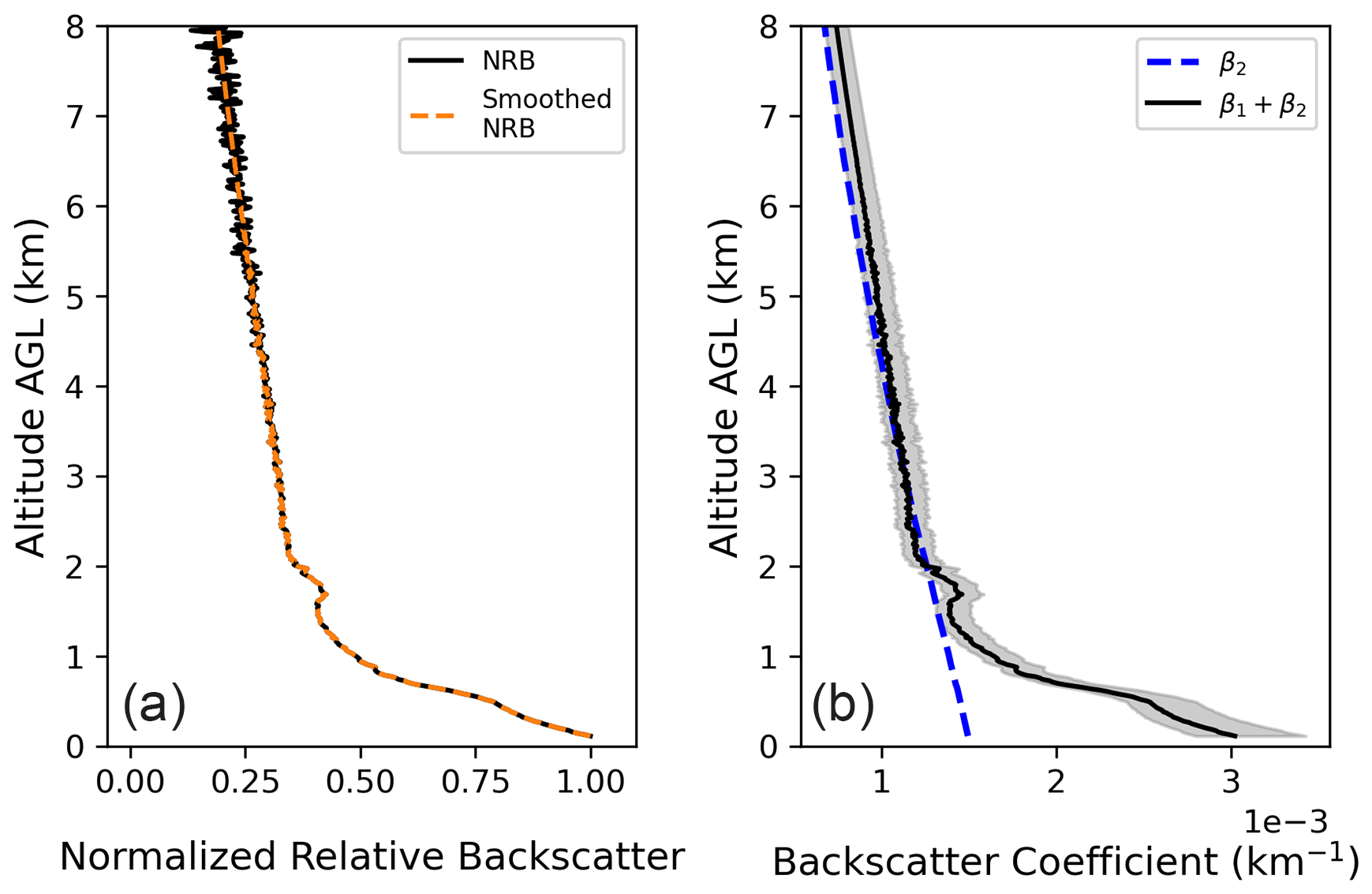
Figure 4 (a) Time-averaged NRB profile of miniMPL from 16:10 to 18:50 UTC on 28 August 2022. The black line is the NRB profile normalized by the lowest level value; the orange dashed line represents the smoothed NRB. (b) Rayleigh backscatter coefficient β₂ (dashed blue line) and total backscatter coefficient β₁+β₂ (solid black line). The shaded region shows the uncertainty range of the retrieved total backscatter coefficient.

An example of NRB profile and backscatter coefficient profile inversion is shown in Fig. 4. The cloud-free NRB profile of miniMPL is time-averaged between 16:10 to 18:50 UTC at Seawolf Park on 28 August 2022. The Rayleigh backscatter coefficient profile, shown in blue dashed lines in Fig. 4b, is calculated using data from the radiosonde launched around 17:30 UTC from the same site, and the total backscatter coefficient derived from the lidar inversion is shown in Fig. 4b as a black solid line. The total backscatter coefficient profile closely follows the molecular (Rayleigh) backscatter profile above 2 km a.g.l., indicating that aerosol contributions are minimal at these altitudes and that the backscatter is dominated by scattering from air molecules. This consistency also suggests that the Fernald inversion is performing well, since the molecular backscatter is independently calculated and provides a reference baseline.

The uncertainty in the total backscatter coefficient is assessed by systematically varying key parameters: the scattering ratio at the calibration height and the lidar ratio. The Fernald inversion process was applied 40 times to the same NRB profile, using 5 calibration scattering ratios (1.0 to 1.2) and 8 lidar ratios (20 to 90 sr), producing 40 backscatter coefficient profiles. The mean of these profiles can be considered as the best estimate, while the spread of these profiles from the maximum to the minimum of these profiles represents the uncertainty interval. This systematic sensitivity analysis ensures that the retrieved aerosol backscatter profile accounts for potential variability in the lidar ratio and the scattering ratio, providing a more reliable estimate. The uncertainty range of the retrieved backscatter coefficient is shown in Fig. 4b as the grey-shaded region.

2.3 Ground-based Aerosol Measurements

During the TRACER field campaign, the TAMU ROAM-V deployed a suite of surface aerosol measurements, which are used in this analysis (see Table 1). The ROAM-V platform shares a heated and dried isokinetic inlet among the TSI Scanning Mobility Particle Sizer (SMPS), the Droplet Measurement Technologies CCN counter, and an additional GRIMM Condensation Particle Counter (CPC). Details of the ROAM-V instrument sampling setup for the TRACER campaign and the particle loss corrections are further described in Thompson et al. (2025a).

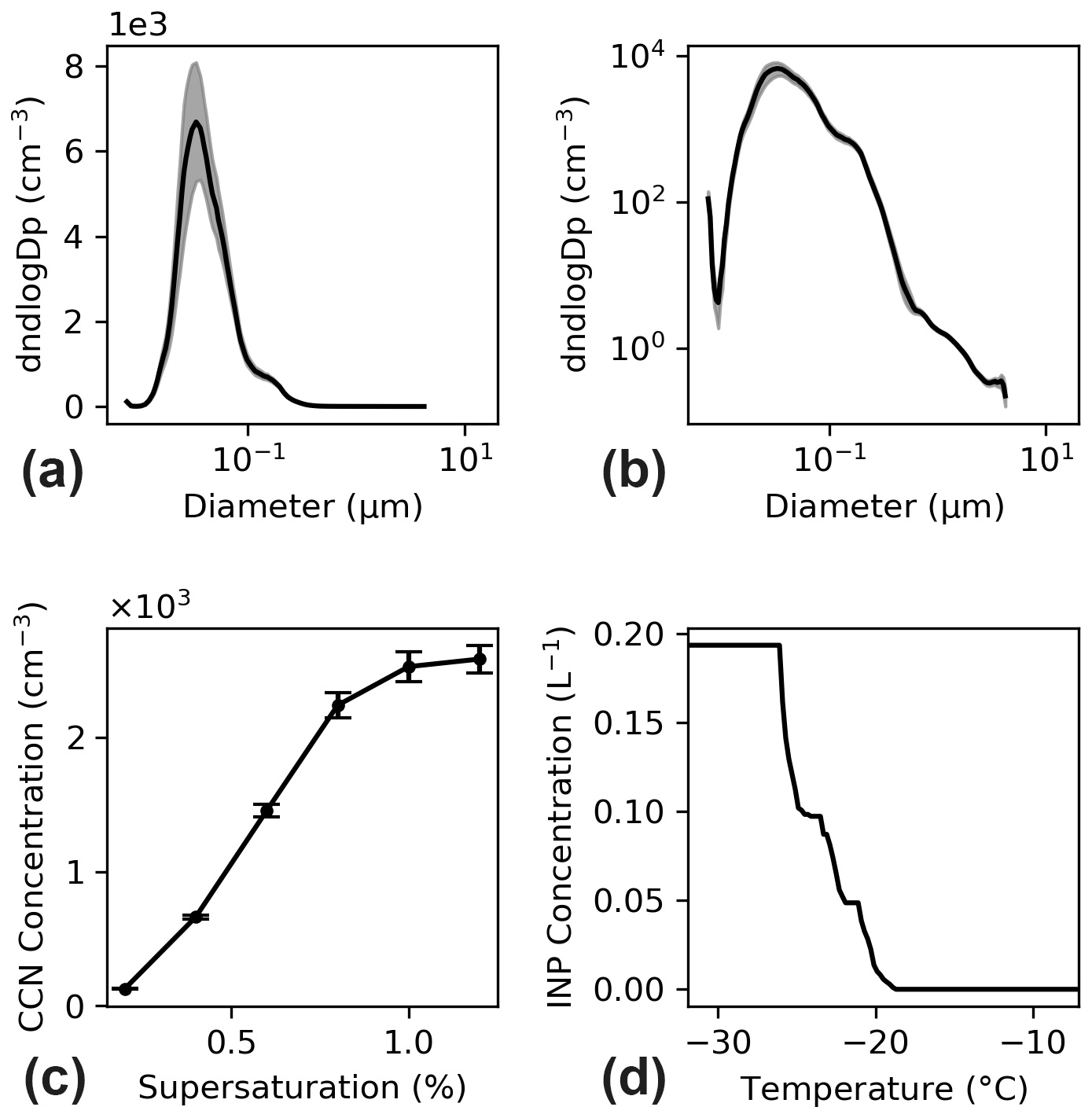
Figure 5 Time-averaged aerosol measurements were collected on 28 August 2022, from 16:10 to 18:50 UTC at the TAMU site in Galveston. (a) Time-averaged aerosol size distribution with a y-axis on a linear scale. The shaded area illustrates the standard error of the estimated mean. (b) Time-averaged aerosol size distribution with a y-axis on a log scale. (c) CCN spectra, where scatter points are time-averaged CCN concentrations at different supersaturations, and the standard error of the sample mean is illustrated as error bars. (d) INP spectra showing INP concentrations evaluated at different temperatures.

Onboard ROAM-V, the SMPS measures the mobility diameter of aerosols between 7 and 305 nm, while the POPS measures the optical diameter of aerosols ranging from 125 to 3370 nm. Because the SMPS and POPS are based on different physical principles, a method was developed to merge their measured size distributions. T-matrix code is used to simulate the signal scattered by quasi-spherical particles of various sizes detected by the POPS, generating a signal-size relation that depends on the aerosol effective refractive index (Mishchenko and Travis, 1994). The POPS-measured aerosol sizes can be recalculated by adjusting the effective refractive index. The refractive index that minimizes the root-mean-square error of the overlapping size region between the POPS and SMPS size distributions is then selected. The resulting POPS size distribution is then merged with the SMPS size distribution by applying a weighted average over the overlapping region. The weights are determined by the Gaussian error function to ensure a smooth transition between the two size distributions. The time average of the merged size distribution across the time-averaging period is used for further analysis. An example of the time-averaged aerosol size distribution measurement taken on 28 August 2022, from 16:10 to 18:50 UTC at Seawolf Park, is shown in Fig. 5a, b. The uncertainty of the aerosol size distribution is represented by two standard errors of the time-averaged aerosol size data to provide a 95 % confidence interval for the time-averaged aerosol size distribution.

The CCN concentration spectra were measured with the CCN counter, which was set to supersaturations between 0.2 % and 1.2 % with intervals of 0.2 %. The CCN counter was calibrated with size-selected ammonium sulfate particles. Similar to the merged aerosol size distribution, the time-averaged CCN spectra are calculated to represent the CCN concentration during the time-averaging period. An example of the average CCN measurement taken on 28 August 2022, from 16:10 to 18:50 UTC at the TAMU site in Galveston, is shown in Fig. 5c. The two standard errors of CCN data are calculated to provide a 95 % confidence interval for the time-averaged CCN concentration.

For ice nucleation measurements, size-resolved aerosol samples were collected using the Davis Rotating-drum Universal-size-cut Monitoring (DRUM) impactor in four size ranges: greater than 3 µm, 3 to 1.2 µm, 1.2 to 0.34 µm, and 0.34 to 0.15 µm, and analysed in the laboratory for ice nucleation measurements. Ice nucleation measurements were conducted using the custom-built immersion freezing array used in our previous experiments (Fornea et al., 2009; Lei et al., 2023; Thompson et al., 2025a; Thompson et al., 2025b), and described only briefly here. Aerosol impactor samples are washed off the impactor substrate into high purity UHPLC (ultra-high-pressure liquid chromatography) water. Then, 2 µL droplets of the sample water are subjected to 25 freeze-thaw cycles on the immersion freezing array. A digital camera is used to detect freezing events and identify ice nucleation temperatures by measuring the average brightness (or grayscale value) of the droplet pixels in an 8-bit image (which has 256 levels of grayscale value). This image-processing technique monitors changes in brightness to infer droplet freezing. The INP concentrations in the air are calculated using established methods (Vali, 1971).

For each retrieval, aerosol, CCN, and INP measurements were averaged over the same one to three hour window as the lidar data used for backscatter profile retrieval. This averaging period reflects the operational constraints of each instrument: the CCN counter requires approximately 30 min to complete a full scan over the range of supersaturations, and INP samples were collected over one to two hour periods (Thompson et al., 2025a).

2.4 Aerosol Hygroscopicity and Lidar Hygroscopic Growth Correction Factor

Since water uptake by aerosols enlarges their size and increases backscattering without affecting aerosol concentration, it is not possible to reliably determine aerosol concentration from the aerosol backscatter profile alone. It is important to convert the aerosol backscatter profile to the aerosol backscatter profile that would be observed under dry conditions prior to calculating aerosol, CCN, or INP concentrations.

In past studies, the hygroscopicity or water uptake by aerosols, defined as the change in aerosol diameter at a given RH relative to its dry diameter, has been quantified by tandem differential mobility measurements (Brooks et al., 2004a; Tomlinson et al., 2007). Similarly, humidified nephelometers have been used to quantify changes in scattering by aerosol at increased RH compared to scattering by dry aerosol, and the results have been used to interpret lidar backscatter observations (Kotchenruther et al., 1999; Ghan et al., 2006).

Here, we developed a new method that combines κ-Köhler theory with Mie theory to infer dry aerosol backscatter profiles from the observations at ambient RH. It is well known that activated CCN are defined as those aerosols that have grown beyond the critical diameter required for spontaneous droplet growth. CCN activation occurs in a supersaturated environment. However, it has been demonstrated that for uniformly mixed soluble aerosol, CCN activation measurements can be used to infer hygroscopic growth of aerosol in subsaturated conditions as well (Petters and Kreidenweis, 2007). This widely used concept has become known as κ-Köhler theory (Petters and Kreidenweis, 2007).

Using κ-Köhler theory, CCN and aerosol size distribution measurements can be combined to infer an aerosol hygroscopicity parameter κ (kappa). The critical dry diameter D_p,c is the size above which dry aerosols of a certain κ activate to form cloud droplets when exposed to a critical supersaturation  SS_c. Following the work of Moore et al. (2011), D_p,c satisfies the integral

$$\begin{array}{}\text{(4)}& N_{\mathrm{CCN}}={\int }_{D_{\mathrm{p},\mathrm{c}}}^{\mathrm{\infty }}{n}_p\left(\log D_{\mathrm{p}}\right)\mathrm{dlog}{D}_{\mathrm{p}}\end{array}$$

n_p(logD_p) is the measured aerosol size distribution in the form of dndlogD_p, and N_CCN is the measured CCN concentration at a supersaturation level. D_p,c can then be numerically solved. Since CCN concentration is measured at a few different supersaturations, multiple pairs of SS_c-D_p,c values are calculated, and an example of the SS_c-D_p,c pairs is shown in Fig. 6a. Each pair of SS_c-D_p,c values can then be numerically solved using κ-Köhler theory to derive a κ value (Petters and Kreidenweis, 2007).

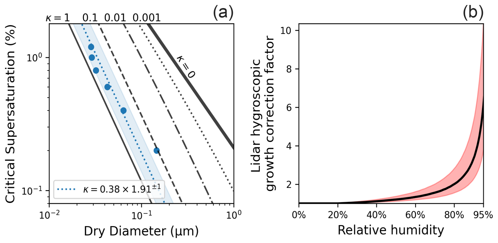
Figure 6 (a) Blue scattered points represent pairs of critical supersaturation and corresponding critical dry diameter derived from aerosol size distribution and CCN measurements. The blue dotted line represents the geometric mean of derived aerosol hygroscopicity κ, and the shaded region represents the one geometric standard deviation of κ. κ= 1 line is shown in a solid black line; κ= 0.1 is shown in a dashed line; κ= 0.01 line is shown in a dash-dotted line; κ= 0.001 line is shown in a dotted line; and κ= 0 is shown in a thick solid black line. (b) Lidar hygroscopic growth correction factor as a function of relative humidity. The shaded area represents the uncertainties of the derived κ.

Following κ-Köhler theory, the saturation ratio S over an aqueous solution droplet with diameter D (also called wet diameter) can be expressed as

$$\begin{array}{}\text{(5)}& S\left(D\right)={\displaystyle \frac{D^{\mathrm{3}}-D_{\mathrm{d}}^{\mathrm{3}}}{D^{\mathrm{3}}-D_{\mathrm{d}}^{\mathrm{3}}(\mathrm{1}-\mathit{\kappa })}}\exp \left({\displaystyle \frac{\mathrm{4}{\mathit{\sigma }}_{\frac{s}{a}}{M}_{\mathrm{w}}}{RT{\mathit{\rho }}_{\mathrm{w}}D}}\right)\end{array}$$

D_d is the dry diameter of the particle. κ is the hygroscopicity parameter. ${\mathit{\sigma }}_{\mathrm{s}/\mathrm{a}}$ is the surface tension of the air-water interface. M_w is the molar mass of water. R is the universal gas constant. T is the temperature evaluated at 298.15 K. ρ_w is the density of water. The κ-Köhler equation relates saturation ratio to particle size, and the supersaturation at the peak indicates the activation point of the particle as a CCN. A numerical function was constructed to find the supersaturation at the peak of the κ-Köhler equation using binary search, with the particle dry diameter and κ as input parameters. Thus, the problem becomes finding the κ corresponding to a given D_p,c as the dry diameter, to match a specific SS_c as the output. The κ is then numerically determined using an iterative root-finding method to match the measured SS_c-D_p,c pairs.

Since κ can be considered as log-normally distributed (Su et al., 2010), the geometric mean and geometric standard deviation can be calculated to represent the average value and the variability of κ for the bulk aerosol composition. An example of the geometric mean and geometric standard deviation of κ is also shown in Fig. 6a. The variation in κ values at different supersaturations can be attributed to uncertainties in measurements and the differences in the aerosol chemical composition and mixing state across various sizes. Subsequently, the aerosol size growth is predicted by numerically solving for the wet aerosol diameter at a discrete series of RH values (Petters and Kreidenweis, 2007). To determine the wet diameter at each RH value, we solve for the point at which the saturation ratio predicted by the κ-Köhler theory matches the specified environmental saturation ratio. This is done through an iterative root-finding approach, using the dry diameter as the initial guess.

Once the aerosol size is known as a function of RH, the Mie scattering theory is then used to calculate the aerosol extinction coefficient at each RH value (Prahl, 2023). The refractive index for dry aerosol is assumed to be 1.45–0i based on values for dry ammonium sulfate at 532 nm (Cotterell et al., 2017). In the absence of detailed aerosol composition data, the refractive index of ammonium sulfate is frequently adopted as a representative value in aerosol optical calculations, as it provides a reasonable approximation for non-absorbing, hygroscopic particles (Zieger et al., 2013; Ghan and Collins, 2004). In reality, aerosols containing sulfate, nitrate, organic compounds, soot, and soil dust were all presented in Houston in varying proportions depending on air mass origin (Thompson et al., 2025a; Lei et al., 2025). The refractive index of aerosol at each RH is calculated as the volume-weighted average of the dry aerosol refractive index and that of water. During the field campaign, aerosol size distribution measurements are made after the sample air is dried to below 30 % RH, as measured by an RH sensor. At this RH level, aerosols are typically considered dry based on the efflorescence point of background ammonium sulfate (Onasch et al., 1999). Therefore, a lidar hygroscopic growth correction factor f(RH) can then be calculated as:

$$\begin{array}{}\text{(6)}& f\left(\mathrm{RH}\right)=\left\{\begin{array}{ll}\frac{\mathit{\sigma }\left(\mathrm{RH}\right)}{\mathit{\sigma }\left(\mathrm{30}\mathit{\%}\right)}& \mathrm{RH}>\mathrm{30}\mathit{\%}\\ \mathrm{1}& \mathrm{RH}\le \mathrm{30}\mathit{\%}\end{array}\right.\end{array}$$

Following the work of Geisinger, the extinction coefficient σ, rather than the backscatter coefficient, was used here. The extinction coefficient is more stable numerically than the backscatter coefficient in Mie scattering calculations and is less sensitive to uncertainties in particle size distribution and refractive index (Geisinger et al., 2017). This is convenient since we already assumed a linear relation between backscatter and extinction in the lidar inversion, and it is justifiable based on the work of Ghan and Collins (2004), in which the influence of RH on backscatter and extinction was shown to be similar. In addition, we assume a perfectly internally mixed aerosol distribution, and we apply the same κ across all aerosol sizes when predicting aerosol size growth at different RH. To account for the uncertainty of κ, we calculate the f(RH) using the geometric mean κ and its value at one geometric standard deviation interval. The f(RH) calculated using the κ values is shown in Fig. 6b. The solid black line represents the f(RH) calculated using the geometric mean κ, and the shaded region represents the f(RH) uncertainty calculated using one geometric standard deviation interval of κ. The calculated f(RH) is further interpolated using a cubic spline to calculate f(RH) at any RH value.

2.5 Deriving the Aerosol, CCN, and INP Vertical Profiles

To retrieve aerosol, CCN, and INP vertical profiles, we assume that the surface measurements are representative of the aerosol size distribution, composition, and cloud-activating ability aloft. This assumption generally holds in well-mixed layers but may break down in the presence of elevated aerosol layers, such as transported smoke or dust, which can be identified in the normalized relative backscatter (NRB) signal. Assuming that aerosol hygroscopicity at the surface is representative of the entire profile, the dry aerosol backscatter coefficient profile β_dry(R) is given by

$$\begin{array}{}\text{(7)}& {\mathit{\beta }}_{\mathrm{dry}}\left(R\right)={\displaystyle \frac{{\mathit{\beta }}_{\mathrm{1}}\left(R\right)}{f\left(\mathrm{RH}\right)}}\end{array}$$

Figure 7a shows the aerosol backscatter coefficient profile (black line with gray shading for uncertainty), the RH profile (solid blue line), and the resulting dry aerosol backscatter coefficient profile (red line with red shading for uncertainty). The radiosonde has a relatively small uncertainty in RH measurements, specified as ±5 %. The uncertainty in the lidar hygroscopic growth correction factor, f(RH), is included in the overall uncertainty of the dry aerosol backscatter coefficient. Assuming that the aerosol, CCN, and INP properties at the surface are representative of the vertical profile, the aerosol (N_p), CCN (N_CCN), and INP (N_INP) concentration profiles can therefore be estimated as:

$$\begin{array}{}\text{(8a)}& {\displaystyle }{N}_{\mathrm{p}}\left(R\right)={\displaystyle \frac{{\mathit{\beta }}_{\mathrm{dry}}\left(R\right)}{{\mathit{\beta }}_{\mathrm{dry}}\left(R_{\mathrm{0}}\right)}}\cdot N_{\mathrm{p}}\left(R_{\mathrm{0}}\right)\text{(8b)}& {\displaystyle }{N}_{\mathrm{CCN}}(R,\mathrm{SS})={\displaystyle \frac{{\mathit{\beta }}_{\mathrm{dry}}\left(R\right)}{{\mathit{\beta }}_{\mathrm{dry}}\left(R_{\mathrm{0}}\right)}}\cdot N_{\mathrm{CCN}}(R_{\mathrm{0}},\mathrm{SS})\text{(8c)}& {\displaystyle }{N}_{\mathrm{INP}}(R,T)={\displaystyle \frac{{\mathit{\beta }}_{\mathrm{dry}}\left(R\right)}{{\mathit{\beta }}_{\mathrm{dry}}\left(R_{\mathrm{0}}\right)}}\cdot N_{\mathrm{INP}}(R_{\mathrm{0}},T)\end{array}$$

R₀ is the altitude where the surface measurements are collected. β_dry(R₀) is the dry aerosol backscatter coefficient profile at R₀. N_p, N_CCN, and N_INP are aerosol, CCN, and INP number concentrations, respectively. One profile each for aerosol, CCN, and INP is retrieved for each time-averaging period. Since the MPL and the miniMPL have near-field blind ranges of 250 and 100 m, respectively, lidar measurements near the surface are unavailable. To estimate the aerosol backscatter coefficient profile within the lidar's blind zone, we perform a second-degree polynomial fit to the dry aerosol backscatter profile from up to 300 m a.g.l. down to the edge of the blind zone. This fitted curve is then extrapolated into the blind zone. Since the aerosol profile is later linearly scaled by the dry backscatter profile, having a physically reasonable estimation of the aerosol profile in the blind zone is necessary to ensure that the scaling reflects realistic near-surface conditions. The extrapolated portions of the dry backscatter coefficient profile within the blind zone are shown as dotted lines in Fig. 7a. The SS is the supersaturation at which the CCN concentration is evaluated, and T is the temperature at which the INP concentration is evaluated. In addition, one standard error of the time-averaged aerosol and CCN concentration of the time averaging period, around one to three hours, is included in the calculation for aerosol and CCN concentration profiles. The aerosol and CCN concentrations evaluated at different supersaturations are shown in Fig. 7b. INP profiles are shown in Fig. 7c. The dry aerosol backscatter coefficient profile determines the shape of aerosol, CCN, and INP concentration profiles, while the surface aerosol measurements determine the amplitude. CCN concentration profiles are presented at different supersaturations, and INP concentration profiles are presented at different activation temperatures. Presenting CCN and INP profiles this way is useful for modeling applications, as it allows the model to compute CCN and INP activation dynamically when the particles are transported to conditions supportive of cloud condensation or ice nucleation within the modeled convection (or other atmospheric processes of interest).

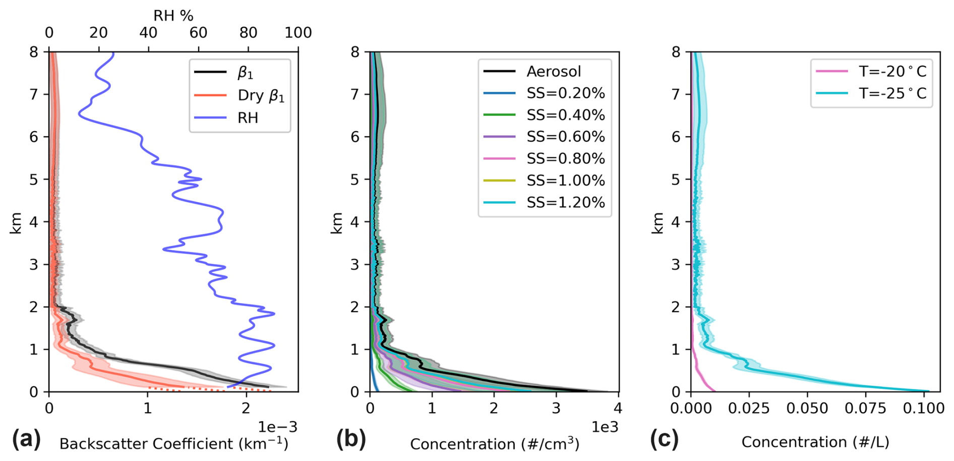
Figure 7 (a) Aerosol and dry aerosol backscatter coefficient profiles are shown as solid black and red lines, respectively, with shaded areas showing the corresponding uncertainty interval for each profile. The relative humidity profile is shown as a solid blue line. (b) The aerosol profile is shown as a solid black line. CCN profiles are shown in different colors corresponding to supersaturation levels of 0.2 %, 0.6 %, and 1.2 %. (c) INP profiles evaluated at −20 and −25 °C.

It is important to acknowledge that lidar-derived aerosol profiles may be affected by the artificial increase in aerosol backscatter at higher altitudes. As seen in Fig. 7a, b, the aerosol backscatter coefficient shows a steady increase with height above 4 km. This apparent increase is likely a systematic artifact related to lidar signal noise at higher altitudes. As a result, the retrieved aerosol profile above 4 km should be interpreted with caution.

3 Results

3.1 Case study: Aerosol Profile under Clear Sky Conditions

We begin with a case study from 31 August 2022, at the coastal Galveston site (16:39–19:00 UTC), representing a baseline case under well-mixed atmospheric conditions with minimal cloud influence. The NRB time series in Fig. 8a shows a persistent layer of high backscatter, visible below approximately 1 km a.g.l. In addition, intermittent layers of high backscatter are observed between 1 and 3 km.

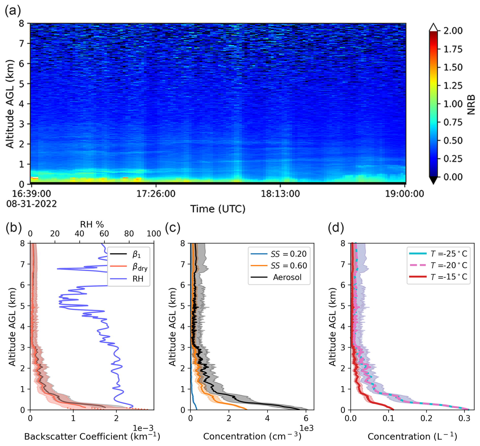
Figure 8 (a) NRB time series data collected on 31 August 2022, from 16:39 to 19:00 UTC, with miniMPL in Galveston, Texas. (b) Aerosol and dry aerosol backscatter coefficient profiles are shown as solid black and red lines, respectively, with a shaded area showing the corresponding uncertainty interval for each profile. The relative humidity profile is shown as a solid blue line. (c) The aerosol profile is shown as a solid black line. CCN profiles are shown in different colors corresponding to supersaturation levels of 0.2 % and 0.6 %. CCN data for 1.2 % supersaturation were not available. (d) INP profiles at −15, −20, and −25 °C. Note that the −20 °C INP profile overlaps with the −25 °C INP profile.

Figure 8b shows the cloud-free aerosol backscatter coefficient and the dry aerosol backscatter profile during the time-averaging period. The relative humidity (RH) profile is relatively uniform below 8 km, stabilizing around 65 %, and the derived aerosol hygroscopicity parameter κ is modest, with a geometric mean of approximately 0.09 × 2.70^±1. This low κ value suggests the aerosol population during this period was only weakly hygroscopic. As expected, under these uniform RH and composition conditions, the correction for aerosol hygroscopic growth introduces minimal differences between the raw and dry backscatter profiles. The similarity between the two profiles (Fig. 8b) confirms that, in this case, the lidar backscatter signal is not significantly biased by water uptake.

Figure 8c shows the retrieved aerosol profile and CCN profile at different supersaturations. Surface aerosol concentrations were (5.65 ± 0.46) × 10³ cm⁻³, decreasing to (1.14±0.57) × 10³ cm⁻³ at 1 km a.g.l., a roughly fivefold reduction with height. CCN concentrations at a supersaturation of 0.2 % show a similar decline, from 329 ± 2 cm⁻³ at the surface to 67 ± 26 cm⁻³ at 1 km. Figure 8d shows the retrieved INP profile evaluated at different temperatures. INP concentrations evaluated at −15 °C were 0.11 L⁻¹ at the surface and 0.02 L⁻¹ at 1 km a.g.l.

3.2 Case study: Correction for Hygroscopic Growth in the Boundary Layer

This case from 6 September 2022 at the inland site in Hockley, Texas (18:30–20:30 UTC), demonstrates the importance of applying a hygroscopic growth correction when RH varies strongly with altitude. Figure 9a shows the lidar NRB time series, with a shallow boundary cloud observed around 1.2 km a.g.l. The layer at and below the cloud level height can be identified as a convective mixed layer, while the layer above the cloud level can be identified as an elevated aerosol layer. Although an elevated aerosol layer exists, it does not affect the correction for the enhanced scattering from hygroscopic growth in the mixed layer. The NRB time series in Fig. 9a shows limited temporal variation in attenuated backscatter profiles during the cloud-free period.

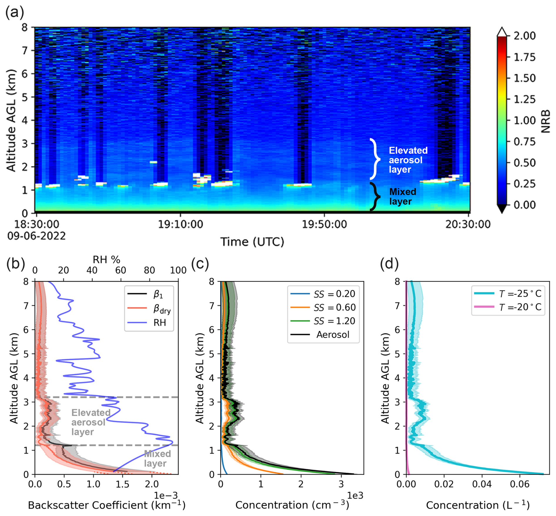
Figure 9 (a) NRB time series data collected on 6 September 2022, from 18:30 to 20:30 UTC, with miniMPL inland at Hockley, Texas. (b) Aerosol and dry aerosol backscatter coefficient profiles are shown as solid black and red lines, respectively, with a shaded area showing the corresponding uncertainty interval for each profile. The relative humidity profile is shown as a solid blue line. (c) The aerosol profile is shown as a solid black line. CCN profiles are shown in different colors corresponding to supersaturation levels of 0.2 %, 0.6 %, and 1.2 %. (d) INP profiles evaluated at −20 and −25 °C. No INP was observed at −15 °C.

Figure 9b shows the cloud-free aerosol backscatter coefficient and the dry aerosol backscatter profile during the time-averaging period. As RH increases toward 100 % within the mixed layer, the correction for hygroscopic growth, applied using the lidar hygroscopicity factor f(RH), results in a dry aerosol backscatter profile lower than the uncorrected one. Without this correction, aerosol concentrations would be substantially overestimated. For example, at 1.2 km a.g.l., aerosol concentration estimates from uncorrected backscatter would exceed the corrected value by a factor of 2.8.

Figure 9c and d show retrieved aerosol, CCN, and INP profiles. The aerosol concentration at the surface is approximately (3.30 ± 0.09) × 10³ cm⁻³ and decreases to 371  216 cm⁻³ at the top of the mixed layer at 1.2 km a.g.l. The CCN concentration evaluated at a supersaturation of 0.2 % is 159 ± 2 cm⁻³ at the surface and 18 ± 10 cm⁻³ at 1.2 km a.g.l. (Fig. 9d). The INP concentration evaluated at −20 °C is around 0.07 L⁻¹ at the surface level and around 3 × 10⁻³ L⁻¹ at 1 km a.g.l. No INP was observed at −15 °C. Between 1.2 and 3.2 km, the dry aerosol backscatter coefficient profile indicates the presence of an elevated aerosol layer above the mixed layer. The aerosol population in the mixed layer and the elevated aerosol layer may differ in terms of aerosol size distribution and chemical composition, making this method for retrieving aerosol, CCN, and INP profiles more uncertain in the elevated aerosol layer shown in Fig. 9. The increase of the dry aerosol backscatter profile as well as the aerosol concentration profile between 6 and 8 km is likely a systematic artifact related to the lidar noise at high altitude.

3.3 Case study: Retrieval of Aerosol Profile with Multiple Cloud Layers

This case from 26 August 2022 at the Galveston coastal site (16:02–18:42 UTC) illustrates the retrieval method's performance in the presence of multiple cloud and moisture layers. In Fig. 10a, cloud layers around 0.6, 1.5, and 3.6 km a.g.l. can be identified as white pixels with high NRB. These cloud layers also match vertical regions of increased RH measured by the radiosonde launched around 17:26 UTC (Fig. 10b). The high attenuated backscatter signal near the cloud levels may reflect the presence of distinct aerosol layers or result from higher humidity enhancing aerosol scattering. The NRB time series in Fig. 10a shows some temporal variation in the attenuated backscatter profile, with a layer of high backscatter slowly decreasing from around 2 to 1 km a.g.l.

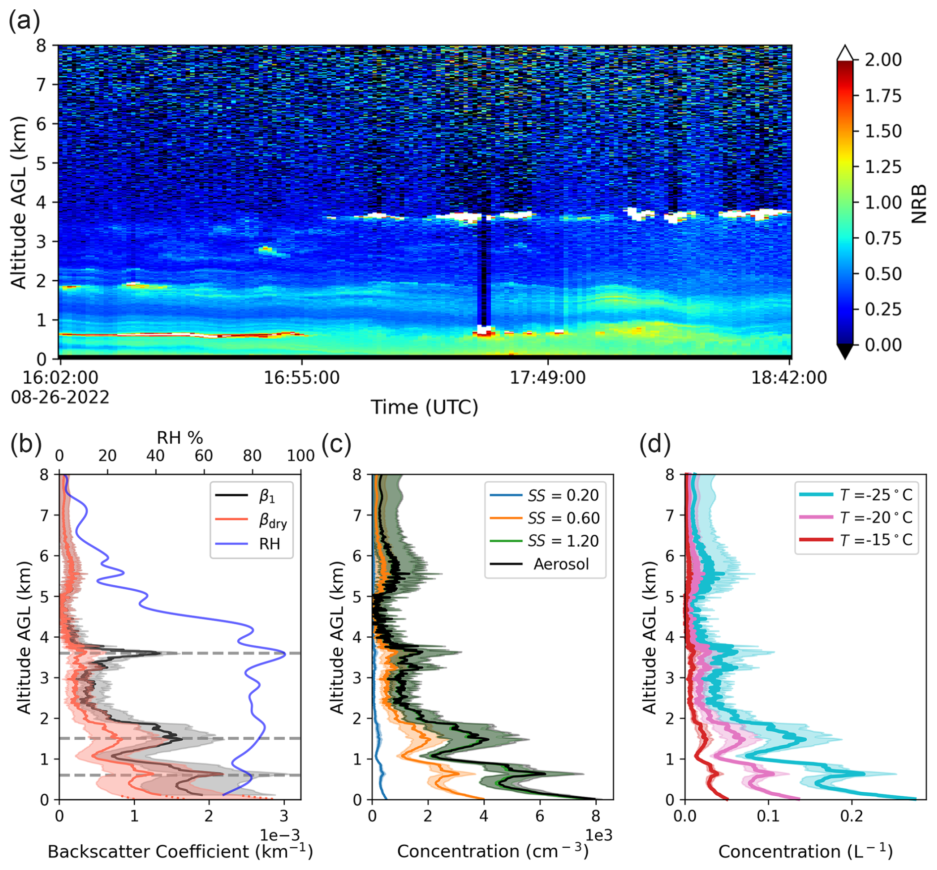
Figure 10 (a) NRB time series collected on 26 August 2022, from 16:02 to 18:42 UTC, with miniMPL in Galveston, Texas. (b) Aerosol and dry aerosol backscatter coefficient profiles are shown as solid black and red lines, respectively, with a shaded area showing the corresponding uncertainty interval for each profile. The relative humidity profile is shown as a solid blue line. Gray dashed lines indicate the cloud level. (c) The aerosol profile is shown as a solid black line. CCN profiles are shown in different colors corresponding to supersaturation levels of 0.2 %, 0.6 %, and 1.2 %. (d) INP profiles at −15, −20, and −25 °C.

As shown in Fig. 10b, a peak in the aerosol backscatter coefficient profile is seen around 3.6 km a.g.l., showing a region where aerosols take up water and grow. This peak is almost completely removed in the dry aerosol backscatter coefficient profile in Fig. 10b, indicating a successful correction for the hygroscopic growth effect on aerosol scattering. This result also demonstrates that the lidar hygroscopic growth correction factor derived from surface measurements can be applied to aerosol aloft. Increased aerosol backscatter coefficients around 0.6 and 1.5 km a.g.l. due to hygroscopic growth are also reduced, resulting in a more realistic aerosol vertical distribution. The dry backscatter profile suggests that an elevated aerosol layer may be present near 1.5 km a.g.l., while the uncorrected peak at 3.6 km a.g.l. is likely dominated by humidity-enhanced scattering rather than a distinct aerosol layer.

Figure 10c and d show retrieved aerosol, CCN, and INP profiles. At the surface, the aerosol concentration is (7.95 ± 0.27) × 10³ cm⁻³, and decreases by approximately 28 % at 0.6 km, 50 % at 1.5 km, and 79 % at 3.6 km a.g.l. At a supersaturation of 0.2 %, the CCN concentrations are 511 ± 10 cm⁻³ at the surface, 368 ± 73 cm⁻³ at 0.6 km, 256 ± 86 cm⁻³ at 1.5 km, and 107 ± 82 cm⁻³ at 3.6 km a.g.l. At a temperature of −15 °C, the INP concentrations are around 0.05 L⁻¹ at the surface, 0.04 L⁻¹ at 0.6 km, 0.03 L⁻¹ at 1.5 km, and 0.01 L⁻¹ at 3.6 km a.g.l. The correction for the aerosol hygroscopic growth leads to the more realistic aerosol, CCN, and INP profiles shown in Fig. 10c, d. The retrieval of aerosol, CCN, and INP concentrations may be less reliable around 1.5 km due to the possible presence of an elevated aerosol layer. However, the successful removal of the humidity-enhanced scattering peak near 3.6 km is encouraging, suggesting that the applied κ value may be reasonable throughout the column.

The increase in the dry aerosol backscatter and aerosol concentration between 5 and 7 km is a systematic artifact likely caused by high lidar signal noise, as shown in Fig. 10a above 5 km. The magnitude of this artifact is likely amplified by the high noise level, which is caused by the limited number of cloud-free profiles available for averaging during this period, as compared to the previous case, where more cloud-free profiles led to reduced noise and less pronounced artifacts.

3.4 Comparison Between Collocated MPL and miniMPL Lidar

The TAMU ROAM-V was deployed at the AMF1 (La Porte, Texas) site on 1 September 2022, allowing miniMPL and MPL to be collocated and compared directly. The ARM MPL deployed at AMF1 collects data at a vertical resolution of 15 m and a temporal resolution of 10 s (Muradyan et al., 2021). During the colocation test, the two lidars were separated horizontally by approximately 30 m and vertically by less than 10 m. The data from both lidars were time-averaged between 20:00 and 22:00 UTC. Vertical profiles of the lidar raw signal, the NRB, and the aerosol backscatter coefficient, and a comparison of the lidar aerosol backscatter coefficient are shown in Fig. 11a, b, c, and d, respectively. Figure 11a shows that the raw signals from the two lidars differ significantly. However, after applying lidar-specific afterpulse, deadtime, background, and range corrections for each lidar, their NRB profiles agree closely (Fig. 11b). Figure 11c and d show that the MPL and miniMPL NRB and aerosol backscatter coefficient profiles follow similar shapes and magnitudes. The miniMPL overestimates aerosol backscatter coefficients between 6 and 8 km compared to the MPL, suggesting that the miniMPL-derived profiles may be less reliable at higher altitudes. This artifact is consistent with the spurious high-altitude enhancements discussed earlier and is likely caused by signal noise and overlap correction uncertainty in the miniMPL retrieval. The miniMPL and MPL profiles exhibit a slight vertical offset below 4 km, which may result from residual errors introduced during the afterpulse, background, or overlap corrections. The differences between the two aerosol backscatter profiles generally remain within the estimated uncertainty bounds, which primarily arise from the assumed lidar ratio and the scattering ratio at the reference height. In summary, miniMPL and MPL data are remarkably similar despite differences in their lidar designs and specifications. This agreement suggests that the more compact and less expensive miniMPL can provide comparable data quality to the more established MPL system. In addition, the use of two lidars with comparable outputs enables coordinated deployment and consistent analysis across different sites over the same period.

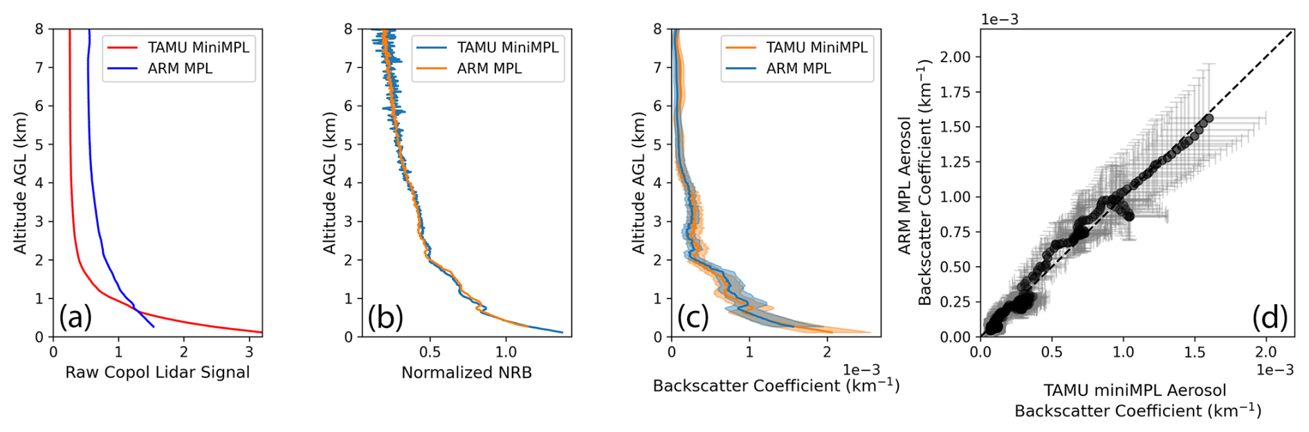
Figure 11 Comparison of retrieved aerosol backscatter coefficient profiles derived from miniMPL and ARM AMF1 MPL data. (a) Raw co-polarized lidar signal of TAMU miniMPL (red solid line) and ARM MPL (blue solid line). (b) Calibrated lidar normalized relative backscatter signal of TAMU miniMPL (red solid line) and ARM MPL (blue solid line). (c) Retrieved lidar aerosol backscatter coefficient of TAMU miniMPL (orange solid line and area) and ARM MPL (blue solid line and area). (d) Comparison of the lidar aerosol backscatter coefficients. The uncertainty interval of the retrieved aerosol backscatter coefficient is shown as error bars.

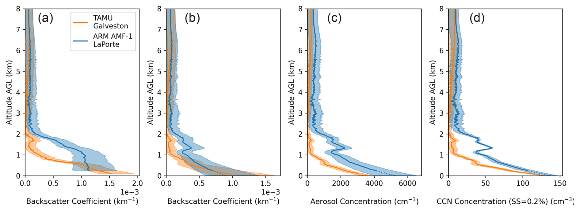
Figure 12 Comparison of lidar measurement of miniMPL deployed at TAMU Galveston site and MPL deployed at ARM AMF1 site on 28 August 2022, from 16:10 to 18:50 UTC. (a) Aerosol backscatter coefficient profiles. (b) Dry aerosol backscatter coefficient profiles. (c) Aerosol concentration profile. (d) CCN concentration profiles at 0.2 % supersaturation.

3.5 Comparison of aerosol and CCN profiles between Galveston and La Porte, Texas (28 August 2022)

A comparison between miniMPL and ARM MPL measurements at different locations at the same time on 28 August 2022 is shown in Fig. 12. miniMPL was deployed at Seawolf Park, Galveston, Texas, and the AMF1 was located in La Porte, Texas. The straight-line distance between the two sites is about 46 km. The time-averaging period was from 16:10 to 18:50 UTC. As shown in Fig. 12b, near the ground surface, the dry aerosol backscatter coefficients at the two sites are similar. The dry aerosol backscatter coefficient at the TAMU Galveston site near the surface is (1.07 ± 0.57) × 10³ km⁻¹, and at the AMF1 La Porte site, it is (0.89 ± 0.51) × 10³ km⁻¹. The dry aerosol backscatter coefficient is greater at the AMF1 La Porte site at higher altitudes. Figure 12c and d show that the aerosol and CCN (SS = 0.2 %) concentration at the AMF1 La Porte site is consistently greater than at the TAMU Galveston site at all vertical levels. At the surface, the aerosol concentration is (3.49 ± 0.34) × 10³ cm⁻³ for the TAMU site and (5.24 ± 1.26) × 10³ cm⁻³ for the ARM site. At 1 km altitude, these concentrations are 313 ± 169 cm⁻³ and (1.78 ± 0.47) × 10³ cm⁻³ for the TAMU and ARM sites, respectively. In terms of CCN concentrations evaluated at 0.2 % SS at the surface, the TAMU site has a CCN concentration of 127 ± 2 cm⁻³, while the ARM site has a slightly greater concentration of 137 ± 9 cm⁻³. At 1 km altitude, the CCN concentration at the TAMU site is 11 ± 5 cm⁻³, compared to a substantially greater concentration of 46 ± 5 cm⁻³ at the ARM site.

These differences highlight variations in aerosol and CCN distributions between the two locations, especially at upper altitudes. The La Porte site likely has a greater dry aerosol backscatter coefficient and aerosol concentration due to surrounding industrial emissions, while the TAMU Galveston site is more influenced by the maritime air mass. Despite similar surface aerosol and CCN number concentrations, there are clear differences in the aerosol and CCN vertical distribution between the two sites, only about 46 km apart. Such variability underscores the importance of localized aerosol vertical profile measurements in characterizing aerosol vertical distributions when assessing their impact on air quality, weather, and climate. It also highlights the necessity of deploying multiple measurement sites to capture the spatial heterogeneity of aerosol vertical profiles when conducting a field campaign that covers a large study area, especially in regions influenced by heterogeneous sources of emissions and complex airmass interactions.

4 Discussion and Conclusions

In this study, we use data collected during the TRACER campaign to demonstrate a new method of retrieving aerosol, CCN, and INP profiles by integrating mini micropulse lidar measurements with radiosonde and ground-based aerosol measurements, including aerosol size distributions, CCN activation, and ice nucleation measurements. In the future, these measurements can be collected routinely to translate lidar backscatter coefficient profiles to long-term aerosol, CCN, and INP vertical profiles. Further, our method is not limited to the micropulse lidar and can be applied to other single-wavelength elastic or more advanced lidars.

One of the key findings of this study is that correcting aerosol hygroscopic growth is necessary for retrieving realistic CCN and INP concentration profiles. We have shown that using lidar-retrieved backscatter or extinction profiles without correcting for hygroscopic growth can lead to a significant overestimation of the aerosol concentration near the cloud base. To solve this issue, we introduced a method to quantify aerosol scattering enhancement due to aerosol hygroscopic growth. This method for determining the lidar hygroscopic growth correction factor can be used as a complementary approach to the traditional method of using a collocated humidified nephelometer (Ghan et al., 2006).

Another key finding is that aerosol and CCN vertical distributions can significantly vary at small spatial scales, even when similar aerosol and CCN concentrations are measured at the surface, as demonstrated by the comparison between the aerosol vertical profile at the ARM and TAMU sites on 28 August 2022. This variability highlights the importance of considering vertical profiles rather than relying solely on ground-based aerosol measurements when assessing aerosol properties and their impacts on cloud formation. It also highlights the need for localized vertical profile measurements to accurately capture the diverse aerosol characteristics in different regions, particularly in areas with complex emission sources and air mass interactions. Portable lidars, such as the miniMPL lidar, combined with surface aerosol measurements, can be highly effective in providing these localized aerosol vertical profile measurements.

While the method described herein clearly has some distinct advantages, it is subject to several limitations. Since the MPL and miniMPL measurements are noisy at upper altitudes, this method's retrieval above the altitude where the lidar signal is smoothed should be used with caution and can only serve as a best estimate. In addition, since our method relies on the assumption that the aerosol size distribution and composition are similar throughout the vertical column, the retrieved profiles are most reliable within the well-mixed boundary layer. At altitudes where aerosol properties differ significantly from those at the surface, such as in the presence of a transported dust layer in the free troposphere, this method may be less reliable, and the results should be interpreted with caution. Despite these limitations, as measurements of CCN and INP vertical profiles are difficult to obtain and sparse, the results from this method can serve as a significant improvement over the arbitrary aerosol profiles often used in model initialization.

In conclusion, the integration of MPL and ground-based aerosol measurements offers a powerful tool for retrieving detailed vertical profiles of aerosols, CCN, and INPs. The retrieved profiles can serve as inputs to provide realistic aerosol vertical distributions for cloud-resolving models, facilitating the study of aerosol-cloud interactions and aerosol effects on climate.