Evaluating Weather and Chemical Transport Models at High Latitudes using MAGIC2021 Airborne Measurements

High latitude wetland emissions of methane (CH₄) remain a significant source of uncertainty in global methane budgets. At these latitudes, flux estimation approaches, such as atmospheric inversions, are challenged by complex meteorological conditions, limited observational coverage, and uncertainties in atmospheric transport modelling. This study evaluates the performance of various atmospheric transport models and reanalysis datasets using meteorological and CH₄ in-situ measurements collected during the MAGIC2021 campaign near Kiruna, Sweden. Over six days of measurements in August 2021, the ERA5 reanalysis, produced by the European Centre for Medium-Range Weather Forecasts (ECMWF) and providing global atmospheric data, showed better agreement with observations compared to the meso-scale Weather Research and Forecasting (WRF) model, though WRF provided valuable insights into local atmospheric dynamics. Among global simulations of CH₄ mixing ratios, inversion-optimised models which adjust emissions to match observations, achieved the best performance overall particularly when constrained by surface measurements. Regional simulations from WRF coupled with chemistry (WRF-Chem) revealed biases in CH₄ mixing ratios in the boundary layer, suggesting an overestimation of emissions by wetland models. All chemistry-transport models exhibited a positive bias in the stratosphere. Simulations with higher vertical resolution demonstrated an improved representation of vertical CH₄ profiles in the upper layers of the atmosphere. Despite the limited spatio-temporal coverage of the observations, we were able to identify the best performing transport models and to evaluate fluxes from different biogeochemical model parameterisations using the MAGIC2021 high-resolution dataset, demonstrating the utility of in-situ vertical profile datasets for transport and flux model evaluation.

1 Introduction

In recent years, the Earth's climate has been rapidly changing, with significant impacts on polar and sub-polar regions. In the Arctic, the rate of warming was thought to be around twice as fast as the global average until recently (AMAP, 2021; Jansen et al., 2020; Walsh, 2014; Yu et al., 2021), but it is now estimated to be closer to 4 times faster (Rantanen et al., 2022). The amount of greenhouse gas in the atmosphere and the meteorological conditions are essential components of the circumpolar climate system, where positive climate feedback loops are ubiquitous and disruptive (boreal fires Zheng et al., 2023, permafrost Miner et al., 2022; MacDougall, 2021, wetland emissions Zhang et al., 2023, and albedo Hall, 2004; Booth et al., 2024). However, a scarcity of long-term direct observational data in the region has proven to be a challenge for studies aiming to constrain uncertainties and changes in the regional methane cycle (Wittig et al., 2023). In order to understand these changes, climate models are therefore highly relied upon, and direct measurements must be employed to provide an assessment of their performance in modelling mixing ratios of greenhouse gases in the region.

In-situ data at high latitudes mainly come from several surface measurement networks operated by Arctic countries, as depicted in Wittig et al. (2023). In Europe, data collection is coordinated by the Integrated Carbon Observation System (ICOS) network, which comprises several towers stationed in Fennoscandia (few above the polar circle), that measure either in-situ atmospheric mixing ratios or methane fluxes through eddy covariance. mixing ratios are however only measured close to the surface. They are mostly representative of local scales and lack vertical information. Measurements covering larger scales and higher atmospheric layers are crucial for accurately modelling the regional methane budget. Several projects have carried out field measurements of atmospheric methane at high latitudes recently, including campaigns from the NASA ABoVE initiative (Sweeney et al., 2022) or the NASA-ESA joint initiative Arctic Methane and Permafrost Challenge (AMPAC, Miller et al., 2021). This latest project was notably involved in the CoMet 2.0 Arctic campaign set in Canada and Alaska in 2022 (https://comet2arctic.de/, last access: 27 October 2025), and MAGIC2021, set near Kiruna, Sweden (67° N). The study presented here focuses on MAGIC2021 (Crevoisier, 2021), which spanned from 14 to 27 August 2021 and included airborne measurements of meteorological variables and atmospheric methane mixing ratios, combined with weather data sounding. The Monitoring Atmospheric composition and Greenhouse gases through multi-Instruments Campaigns (MAGIC) initiative launched by Centre National de la Recherche Scientifique (CNRS) and Centre Nationale des Études Spatiales (CNES) aims at improving knowledge of CO₂ and CH₄ distribution and emissions in the Earth's atmosphere by organising frequent measurement campaigns in different regions of interest. The first three campaigns, set in France from 2018 to 2020, served as a mean to calibrate and validate instruments and measurement techniques, whilst also validating current space missions. MAGIC2021 was therefore the first MAGIC campaign to focus on the study of CH₄ emissions at high latitudes, bringing together 70 participants from 17 teams and 7 different countries. As field work is relatively recent, few results have been published yet and, to our knowledge, no study has tried to extensively assess atmospheric composition models using campaign data at high resolution in those regions.

Kiruna and its surrounding area are characterised by wetland landscapes that include small ponds to large lakes as well as peatland and various inundated soils found in both boreal forest and tundra ecosystems, as shown on the left panel of Fig. 1, where land cover comes from European Environment Agency (2019). These wetlands are known to be the main local source of methane though their emissions are generally poorly constrained (Saunois et al., 2020). Additionally, some permafrost areas are also present at higher altitudes found in the Scandinavian mountains west of the city, though to a relatively small extent (Brown et al., 1997). In lower parts of the atmosphere, model estimates of greenhouse gas mixing ratios can be strongly affected by these high uncertainties in emission processes, particularly for methane. Boundary layer mixing ratios are also strongly influenced by turbulent flow which is parametrised in global models and challenging to simulate accurately at finer scale (Schuh et al., 2019). This has a strong influence on atmospheric composition at all levels, as CH₄ released at the surface is usually transported to deeper atmospheric levels via turbulent and/or convective fine scale processes. Above the boundary layer, transport by geostrophic wind becomes the major driver for greenhouse gas mixing ratios. This means that atmospheric methane content is no longer strongly dependent on local emissions, but rather influenced by medium to long range transport. Stohl (2004) have shown that mixing ratios observed in Northern Europe can be traced back to emissions from North America or Siberia, provided meteorological conditions allowed for transport of surface emissions to the free troposphere. At higher altitudes, an important driver of CH₄ mixing ratios becomes methane depletion by OH radicals and other molecules (e.g. Cl, Li et al., 2018). Their presence mostly affect methane mixing ratios in the upper troposphere and lower stratosphere, where stratification and reaction with these chemical species reduce drastically CH₄ mixing ratios in the upper troposphere and above the tropopause. Upper-tropospheric and lower-stratospheric CH₄ mixing ratios are therefore characterised by a strong vertical gradient. Tropopause height and troposphere/stratosphere exchanges are thus key influences on CH₄ mixing ratios (Xiong et al., 2013), and are also challenging to model accurately (Mateus et al., 2022).

In this study, the accuracy and precision of several models in reproducing greenhouse gas mixing ratios and meteorological conditions observed at fine scale are assessed. Our study uses in-situ observations that employed research aircraft and weather balloons deployed around Kiruna in August 2021 (details in Sect. 2). We first start by assessing models regarding meteorological variables, with data from the European Centre for Medium-Range Weather Forecasts (ECMWF) fifth-generation reanalysis (ERA5) global product and regional WRF simulations. Then, we assess the atmospheric composition models ability to reproduce observed CH₄ mixing ratios. Models assessed include the Copernicus Atmosphere Monitoring Service (CAMS) analysis hlkx and inversion-optimised flux product version 21r1, six PYVAR-LMDz-SACS ensemble inversions and WRF-Chem regional simulations. More detail about these models can be found in Sect. 2. Comparisons between model simulations and observational data provide insights into the strengths and limitations of these models in the Lapland region and highlight areas for improvement at several levels and scales.

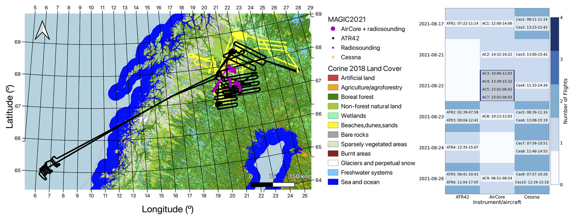
Figure 1 Location (left) and date and time (right) of MAGIC2021 measurements used in this study. Map background shows land use adapted from the Corine2018 dataset (European Environment Agency, 2019). Individual land cover types from the Corine2018 dataset are grouped in broader categories to ease map interpretation. Notably, wetlands include inland marshes, peat bogs, salt marshes, salines, intertidal flats, coastal lagoons and estuaries, i.e. both freshwater and saltwater wetlands.

2 Methods

2.1 Observational data

Both ground-based and airborne measurements were taken during MAGIC2021. This study focuses on airborne data taken by CNES weather balloons as well as two aeroplanes, an ATR42 from SAFIRE and a Cessna from Deutsches Zentrum für Luft- und Raumfahrt (DLR). These platforms had different payload configurations and measurement capabilities and thus provide complementary information about the distribution of gases in the atmosphere. Whilst this study does not make use of the full set of MAGIC2021 measurements due to data availability at the time of our analysis, it provides a solid example of such campaigns capability in terms of model validation. All data were put on the WMO scale (Dlugokencky et al., 2005) through several inter-comparisons and inter-calibrations using similar gas tanks on each Picarro analysers. These were carried out during the campaign, and included a wing-by-wing flight by the ATR42 and Cessna aircraft.

2.1.1 Weather balloon observations

Two types of weather balloons from CNES were released during MAGIC2021: the Light Inflatable Balloon (BLD – Ballon Léger Dilatable) and the Zero Pressure Difference (ZPD) balloon. Balloon types differ in their usage, BLD are single-use, their membrane bursting after the ascent phase. They typically reach altitudes up to 30 km. ZPD are reusable and can reach altitudes above 30 km. Weather balloons carried two main instruments whose data were used in the study: the AirCore atmospheric sampler, and meteomodem M20 radiosondes. The M20 instrument is an ultra-lightweight (36 g) radiosonde used to gather meteorological data such as temperature, humidity, pressure, as well as zonal (U) and meridional (V) wind components. More details about the instrument can be found at https://www.meteomodem.com/m20? (last access: 21 October 2025). Measurements with the M20 were made during both ascending and descending phases of balloon flights.

AirCore is an atmospheric sampler (Tans, 2009; Karion et al., 2010; Membrive et al., 2017) which allows sampling atmospheric composition on a large range of altitudes (∼0–30 km) making use of the atmospheric pressure gradient. To be more specific, the AirCore is made of a coated stainless steel tube that is filled with a calibration gas before release. The length of that tube varies according to the AirCore type: light AirCores have a shorter tube than high resolution AirCores. The sampler is then attached to a weather balloon that is released from the surface. During the ascending phase, the relatively high pressure inside the tube pushes out the calibration gas. At the top of the trajectory, the balloon pops and the payload starts a descending phase during which increasing pressure outside of the tube pushes atmospheric air inside the AirCore. Similarly to ice cores, the resulting sample consists of a continuous profile of atmospheric air, with the most recently sampled air (from lower altitudes) located near the inlet and the earlier sampled air (from higher altitudes) located deeper within the tube. Both light AirCore and high resolution AirCore were deployed during MAGIC2021. After sampling, AirCores were retrieved and analysed on the ground, using the G2401 instrument from Picarro© (Picarro, 2008) which measured CH₄, CO₂, CO and H₂O. Time and trajectories of measurements for the AirCore instrument are shown in Fig. 1. Atmospheric composition observations used in this study include 8 separate weather balloon soundings. For meteorological data, only 6 of the 8 weather balloons were used due to radiosondes malfunctioning during two of the flights, but meteorological data were acquired during both ascent and descent flight phases which allowed to compensate for missing data.

2.1.2 Aircraft observations

Two research aircraft flew between the surface and approximately 8 km, carrying instruments that gathered atmospheric composition and weather data: the SAFIRE ATR 42-320 (CNES, CNRS, Météo France), abbreviated as ATR42, and the DLR Cessna C-208B Grand Caravan, abbreviated as Cessna. The position, velocity, and altitude of the ATR42 aircraft were recorded by both an iXBlue™ inertial reference/navigation system called SAFIRE AIRINS and a NovAtel™ Global Positioning System (GPS). This GPS system consists of L1/L2 GPS-Antennae (5×) and a OEM3 receiver. Water vapour and relative humidity were measured using a non dew/frost point hygrometer called SAFIRE relative humidity sensor, made by Michell Instruments™. Airspeed, incidence angle and turbulence were measured by a Rosemount & Sextant™ incident flow vector probe called SAFIRE five hole radome. This instrument allows the measurement of U and V wind components. Finally, the Rosemount™ in-situ temperature sensor called SAFIRE Rosemount PT102E2AL, measures the temperature at the aircraft's location. Also on board the ATR42 were two Picarro™ models. One was the previously mentioned G2401 and the other was the G5310 that measures CO with higher precision as well as N₂O. Other instruments installed on the aircraft also gathered additional meteorological data.

The Cessna aircraft was equipped with a system called blackMAMBA (Measurement Acquisition of Meteorological Basics) that delivered track (i.e. position and time) data, together with aircraft status and meteorological parameters. Some of the meteorological sensors were installed in the MetPod, a container with a nose boom, mounted under the left wing. This allows atmospheric parameters to be measured with less distortion than if they were measured from the fuselage. The temperature, pressure, humidity sensors and the calibration of the wind measurement system are described in detail by Mallaun et al. (2015). The aircraft also carried two in-situ trace gas instruments. Here we use only the data from a Picarro G1301m, which measured CH₄, CO₂, and H₂O mixing ratios. More details about gas measurements can be found in Fiehn et al. (2020).

Observations used in this study include 6 ATR42 and 10 Cessna flights for both atmospheric composition and meteorological data.

2.2 Atmospheric modelling systems

This section describes model data that was compared to MAGIC2021 observations. The first two sections describe global models whilst the third focuses on the regional modelling system based on WRF-Chem that was specifically set up for MAGIC2021.

2.2.1 Global meteorological reanalysis

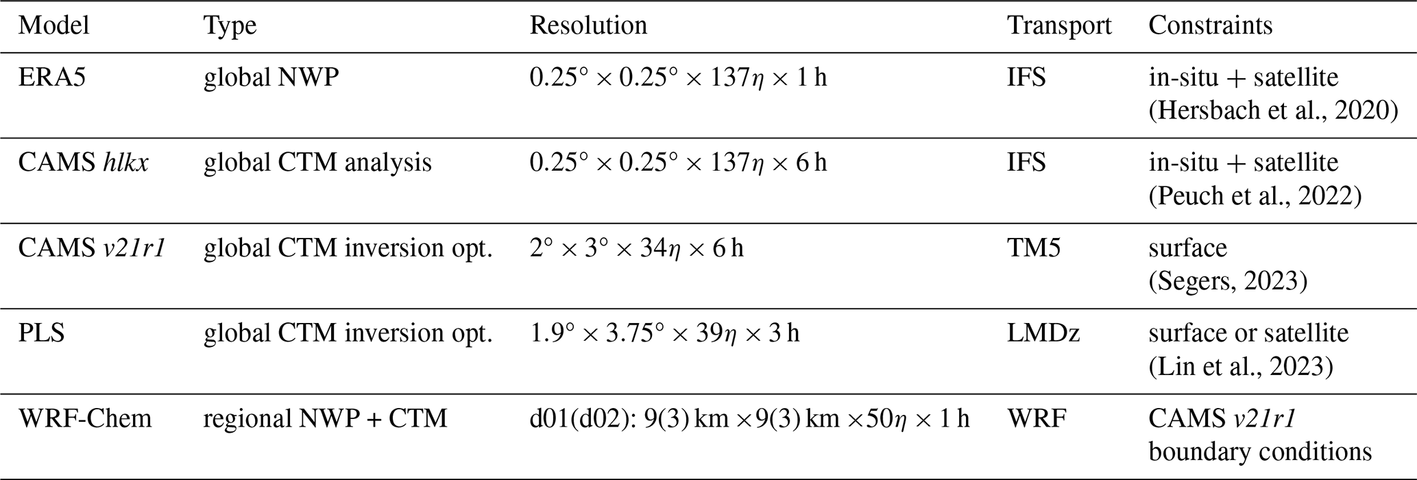
Global meteorological fields used in this study came from the European Centre for Medium-Range Weather Forecasts (ECMWF) fifth-generation reanalysis product (ERA5, Hersbach et al., 2020; C3S, 2018), that provides meteorological data on a global scale from 1950 to present. In our study, we assessed ERA5 reanalysis wind, temperature, and humidity. The high density of vertical levels in ERA5 from the mid-troposphere down to ground level allows for accurate comparison with the flights from MAGIC2021. Our analysis was carried out using ERA5 at time resolution of 1 h, spatial resolution of 0.25° and 137 vertical levels. Horizontal ERA5 wind was given in terms of zonal (U) and meridional (V) components of the wind vector. Both observations and model data were converted to horizontal wind speed V and direction θ for comparison when needed using: $\mathbf{V}=\sqrt{{\mathbf{U}}^{\mathrm{2}}+{\mathbf{V}}^{\mathrm{2}}};\mathit{\theta }={\text{tan}}^{-\mathrm{1}}(-\mathbf{U},-\mathbf{V})\cdot \frac{\mathrm{180}}{\mathit{\pi }}$ (Tetzner et al., 2019). To compare humidity from models (given as specific humidity q in ERA5) to measured relative humidity (RH), ERA5 data was converted to RH using $\text{RH}=\frac{e}{e_{\mathrm{s}}}$ where e is the partial pressure of water vapour in air (pressure exerted by water molecules) and e_s is the saturation vapour pressure, or the maximum vapour pressure achievable at a given temperature before condensation occurs.

2.2.2 Global CH₄ assimilation systems

The Copernicus Atmosphere Monitoring Service (CAMS) is a service provided by ECMWF. Its atmospheric composition product combines satellite data and ground-based measurements in a 4D-Var assimilation system to provide comprehensive information on key atmospheric parameters such as mixing ratios of greenhouse gases in 4 dimensions (Peuch et al., 2022). Two CAMS products are used in this study. The first is the CAMS hlkx analysis (Agustí-Panareda et al., 2023) which is based on ECMWF Integrated Forecast System for Composition (C-IFS, Verma et al., 2017), with a vertical resolution of 137 vertical levels, a horizontal resolution of 0.25° and 6 h of temporal resolution. Methane loss to OH in the upper troposphere and stratosphere is provided by Bergamaschi et al. (2009) where CH₄ destruction was simulated using OH fields based on methyl chloroform optimised Carbon Bond Mechanism 4 (CBM-4) chemistry (Bergamaschi et al., 2005; Houweling et al., 1998). Non-OH stratospheric loss is based on the 2-D photochemical Max-Planck-Institute (MPI) model (Bergamaschi et al., 2009; Brühl and Crutzen, 1993).

The second CAMS product compared to MAGIC2021 is the global inversion-optimised greenhouse gas mixing ratios product for CH₄ version 21r1 (Segers, 2023). This product makes use of methane mixing ratio measurements from the NOAA ground observations network to optimise a priori fluxes of CH₄ and produce 3D mixing ratios and correspond better to ground observations. Simulations are run using the chemistry transport model TM5-MP (Williams et al., 2017) that includes upper tropospheric and stratospheric computation of CH₄ loss using monthly mixing ratios of sink tracers, built-in reaction rates and monthly temperature estimates. Tropospheric or stratospheric reaction rates are attributed using a latitude dependent tropopause parameterisation from Lawrence et al. (2001). The spatial resolution is of 2°×3° (latitude × longitude) ×34 levels and the temporal resolution is 6 h. To distinguish between these two products from CAMS, the analysis product will be referred to as CAMS hlkx and the inversion-optimised product as CAMS v21r1.

Campaign data was also compared to mixing ratios from six PYVAR-LMDz-SACS (Peng et al., 2022; Lin et al., 2024, abbreviated PLS) ensemble inversions that optimised weekly methane surface fluxes for 2021 at a spatial resolution of 1.9°×3.75° on 39 vertical levels and 3 h time resolution. Inversions employed three different atmospheric observation datasets for flux constraints and two physical parameterisations. Two inversions used GOSAT column estimates to constrain fluxes, either from the National Institute for Environmental Studies (NIES) or University of Leicester (UoL) and the others used in-situ measurements from both the Integrated Carbon Observation System (ICOS) and NOAA tower networks. The two physical parameterisation are known as the “classic” and “advanced” versions of the atmospheric transport model LMDz (noted a and b respectively). The “classic” version uses the vertical diffusion scheme of Louis (1979) and the scheme of Tiedtke (1989) to parametrise deep convection, whilst the “advanced” version combines the vertical diffusion scheme of Mellor and Yamada (1974) and thermal plume modelling by Rio and Hourdin (2008) to simulate the atmospheric mixing in the boundary layer. Deep convection is represented using the scheme from Emanuel (1991) coupled with the parameterisation of cold pools developed by Grandpeix et al. (2010). Bottom-up inventories or process-based land surface models were used to build prior CH₄ fluxes for different categories, and the OH and O(¹D) fields were prescribed from the simulation of a chemistry-climate model LMDz-INCA with a full tropospheric photochemistry scheme. Inclusion of observations and definition of observation errors to constrain fluxes followed the method outlined in Peng et al. (2022); Lin et al. (2024).

2.2.3 Regional atmospheric model (WRF-Chem)

WRF-Chem configuration

In addition to global model outputs, the Weather Research and Forecasting coupled with Chemistry (WRF-Chem) model was used to simulate the meteorological conditions and greenhouse gas mixing ratios during the MAGIC2021 campaign on a regional scale. WRF is a widely used mesoscale numerical weather prediction system in both research purposes and operational forecasting. It uses fully compressible and non-hydrostatic Eulerian equations on an Arakawa C-staggered grid to ensure the preservation of mass, momentum, entropy, and scalars (Skamarock et al., 2008). The set-up for this study included two domains, one parent and one nested. The parent domain (d01) encompassed the whole of Fennoscandia as well as Denmark, the westernmost part of Russia and most of the area covered by Baltic countries, at a resolution of 9×9 km. The nested domain (d02) had a higher resolution of 3×3 km and spanned most of the northern part of Finland, Sweden and Norway where MAGIC2021 measurements were taken. Domain boundaries were chosen such as to avoid strong emissions and high topography close to a boundary, which are known to cause transport problems (NCAR, 2024). WRF-Chem generated output fields including meteorological variables and mixing ratios every 20 min.

The physical parameterisation included the WSM5 scheme for microphysics (Hong et al., 2004) as well as the RRTMG longwave and shortwave schemes (Iacono et al., 2008) for radiation. The planetary boundary layer was represented using the MYNN Level 2.5 scheme (Nakanishi and Niino, 2009), whilst the revised MM5 surface layer scheme (Jiménez et al., 2012) was used, with the thermal roughness length dependent on vegetation. No urban model was activated. For the land surface, the Noah model was used, with 4 soil layers (Tewari, 2004). Regarding convection, the Kain-Fritsch scheme was used for the parent domain (Kain, 2004), whilst convection was resolved explicitly in the nested domain. Additional convection-related options were activated, including radiation feedback on convection, convection diagnostics, and Grell-Devenyi scheme parameters (Grell and Dévényi, 2002). Vertically, the simulations had 50 levels from ∼ 140 m to ∼ 20 km with about half of all levels below 2 km. The model configuration was evaluated in previous studies to produce minimum transport errors at both continental (Feng et al., 2019) and regional (Díaz-Isaac et al., 2018) scales.

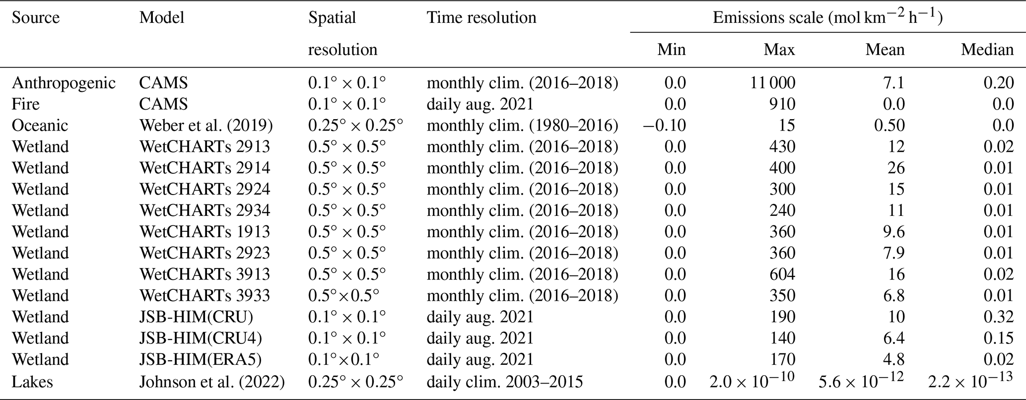
Methane mixing ratios were modelled as passive tracers, which were transported online at each time step concurrently with meteorological variables. Emissions are injected from the surface into the first atmospheric layer to generate the mixing ratio fields of tracers. These tracers undertook a series of transport processes, including advection, diffusion, turbulence, and convective mixing, to simulate the motion of molecules in the atmosphere. Initial conditions were set by ERA5 reanalysis meteorology at $\mathrm{0.5}\mathit{°}\times \mathrm{0.5}\mathit{°}\times \mathrm{137}$ levels resolution and boundary meteorological conditions were updated every 3 h using the same product. Data within WRF-Chem domain was then produced by WRF physics and dynamics. Methane boundary conditions were produced by the inversion optimised CAMS mixing ratios product version 21r1 described earlier, at a resolution of $\mathrm{3}\mathit{°}\times \mathrm{2}\mathit{°}\times \mathrm{34}$ levels every 6 h. Emissions within simulation domains were divided into multiple tracers depending on source types. These tracers are described in Table 1. mixing ratios within our simulation domain were initially set to a constant value. A period of 15 d was shown to be sufficient for boundary conditions and local emissions to propagate through our domains and reach steady-state. The simulations were thus run from 1 to 31 August 2021, to account for spin-up time and the MAGIC2021 campaign period.

Table 1 Emission sources used in the WRF-Chem simulations, given with spatial and temporal resolutions as well as emission statistics. Statistics are computed for the larger (d01) WRF-Chem domain over the month of August 2021 or climatological August depending on data availability.

Emission tracers

Input emissions (Table 1) were chosen according to data availability for August 2021, then prioritising higher spatial resolution in order to reduce regridding issues. If no product were found for that time period, the highest time resolution product was chosen and climatological averages were used.

Oceanic methane emissions were taken from Weber et al. (2019), a monthly climatology with a spatial resolution of 0.25°×0.25°. Methane lake emissions from Johnson et al. (2022) were also used. The dataset includes corrections for daily and seasonal observational bias, observed ice-free/emission seasonality, and realistic lake area and distribution. Anthropogenic and fire emissions of methane were provided by CAMS, which publishes emissions driving their global atmospheric greenhouse gas mixing ratios products (Agustí-Panareda et al., 2023). They are respectively from EDGARv4.2FT2010 (Olivier and Janssens-Maenhout, 2012) and GFAS Version 1.2 (Kaiser et al., 2012). Anthropogenic and fire emissions both share the same 0.1°×0.1° spatial resolution but anthropogenic emissions were monthly averaged emissions over 2016–2017–2018 (latest years available) whereas fire emissions were daily emissions from August 2021. Wetland emissions came from two sources: the latest product from the WetCHARTs model (Bloom et al., 2017), with simulations up to 2019, and several versions of JSBACH-HIMMELI (JSB-HIM) simulations originally designed for the European project VERIFY, described in Aalto (2019), that were recently extended to later years. WetCHARTs has a spatial resolution of 0.5°×0.5° and a monthly time resolution, spanning until 2019. A monthly climatological average was therefore used, taking the same years as for CAMS anthropogenic emissions. 18 different flux versions are publicly available from WetCHARTs, depending on physical parameters detailed in the documentation (Bloom et al., 2017). A subset of 8 WetCHARTs versions were selected, to maximise representativeness of the dataset whilst staying cost-effective in our computations. JSB-HIM emissions were provided by the Finnish Meteorological Institute (FMI) at daily resolution for August 2021 and a spatial resolution of 0.1°×0.1°. 3 versions of total wetland flux from JSB-HIM, each differing in their driving meteorology were included in this study.

Inventory emissions all have different spatial resolution, so they have to be regridded to our WRF-Chem domains resolution. This was done by interpolating emissions from our data products to the WRF-Chem grid (Virtanen et al., 2020). 11 emission tracers and one boundary condition tracer were tracked in the simulation of total regional CH₄ mixing ratios. Boundary conditions were provided by the inversion-optimised CAMS v21r1 product described in Sect. 2.2.2 and interpolated onto WRF-Chem vertical levels using https://github.com/psu-inversion/WRF_boundary_coupling, last access: 27 October 2025. Additionally, artificial boundary conditions were also implemented for other tracers in order to prevent near-zero computation error propagation throughout the whole simulation. This was done by adding a constant offset of 300 ppb through the emission tracers domain boundaries on an hourly basis. WRF-Chem supports several independent passive tracers. This allows us to construct different versions of atmospheric methane mixing ratios from a single simulation. A common core of methane mixing ratios was built using the boundary condition tracer added to the sum of anthropogenic, fire, oceanic and lake emissions tracers. To this common core, wetland contributions can be separately added to obtain different atmospheric methane mixing ratios. These wetland emissions include 8 separate products from the WetCHARTs inventory, and 3 products from JSB-HIM simulations as described above (Bloom et al., 2017; Aalto, 2019). Simulations were run in both d01 and d02 domains, resulting in a total of 22 atmospheric CH₄ mixing ratios product.

Table 2 Model specifications for simulations used in this study. η vertical coordinates are a hybrid sigma-pressure coordinate. Meteorologicalonstraints can be from in-situ measurements such as weather balloons or measurement towers. For CH₄ we use surface to specify that constraints come from surface mixing ratio measurements.

2.3 Comparison method

2.3.1 4 dimensional barycentric interpolation using Delaunay triangulation

In our comparisons, modelled data were interpolated on measurement locations using the python function scipy.interpolate.griddata from the scientific python library scipy. The function griddata uses scipy.interpolate.LinearNDInterpolator when performing linear interpolation in multiple dimensions as in our case, a function that was written in cython by Virtanen et al. (2020). Interpolation is necessary because gridded modelled data do not have the same temporal or spatial resolution as measurements taken by balloons or aircraft. Additionally, using Delaunay triangulation as in griddata allows interpolation from an irregular grid such as the pressure grid used in studied models. The interpolation was performed in 4 dimensions (time + 3 space dimensions). griddata first computes a Delaunay triangulation around the measurement coordinates to pick out interpolating points from the model grid. In 4 dimensions, each simplex around an observation point contains 5 vertices corresponding to 5 model coordinates in 4D. Barycentric linear interpolation is then performed using each simplex's 5 vertices to compute a model value at a particular measurement location. This method enables a fast, easy to implement and accurate comparison between modelled and measured data, by allowing comparison along each instrument's individual trajectory.

2.3.2 Layer analysis and statistical metrics

Our analysis systematically divided comparisons in 3 layers: the boundary layer (BL), free troposphere (FT) and lower stratosphere (LS). MAGIC2021 data and interpolated model data was categorised as within the BL if the measurement height was below the BL height as computed by ERA5, interpolated at the measurement location. The FT layer extended from the BL height up to the tropopause, which was only reached by weather balloons. Tropopause height was derived from observational data using the cold-point tropopause (CPT) method (Eugenio and Macalalad, 2021).

Four statistical metrics were computed to assess model performance against observations in each of the three previously defined layers and to compare the performance of models. In the following, we note the model bias $\stackrel{\mathrm{‾}}{\mathrm{\Delta }}$ from Willmott (1982), which is the mean difference between interpolated model quantities and measured physical quantities over a sample of measurements, standard deviation σ, Pearson correlation ρ, and root-mean-square error RMSE. Circular statistics from Mardia (1972); Jammalamadaka and Sengupta (2001) were applied to compare wind directions by computing circular $\stackrel{\mathrm{‾}}{\mathrm{\Delta }}$, σ, ρ and RMSE associated with model and observed directions.

These metrics were used to draw Taylor diagrams (Taylor, 2001) which allow to assess a set of models against observations. These diagrams cleverly combine ρ, σ and centred RMSE (CRMSE) in a polar coordinate plot using the law of cosines. The radial coordinate of a data point usually represents the standard deviation (r=σ) whilst angular position gives its correlation with observations (α=arccos(ρ)). A reference point is set at (σ_obs, ρ_obs) where σ_obs is the standard deviation of the observations and ρ_obs=1. Here we normalise σ to be able to compare quantities from different layers of the atmosphere onto the same plot: ${\mathit{\sigma }}_{\text{N}}=\mathit{\sigma }/{\mathit{\sigma }}_{\text{obs}}$. The coordinates of the reference point become (1,1). The better the model, the closer to this reference point it will be. CRMSE can also be represented on the diagram, as the radial distance from the reference point. Taylor (2001) shows:

$$\begin{array}{rl}\text{CRMSE}& =\sqrt{{\displaystyle \frac{\mathrm{1}}{N}}\sum _i^N{\left[(x_i^{\text{obs}}-\stackrel{\mathrm{‾}}{x^{\text{obs}}})-(x_i^{\text{mod}}-\stackrel{\mathrm{‾}}{x^{\text{mod}}})\right]}^{\mathrm{2}}}\\ & =\sqrt{{\mathit{\sigma }}_{\text{obs}}^{\mathrm{2}}+{\mathit{\sigma }}_{\text{mod}}^{\mathrm{2}}-\mathit{\rho }{\mathit{\sigma }}_{\text{obs}}{\mathit{\sigma }}_{\text{mod}}}\end{array}$$

This metric is a measure of model spread around observational values after removing any bias. It is therefore useful to quantify model noise but it lacks an assessment of distance between model estimates and observations. To remedy this, we chose to pair each Taylor diagram with a plot of RMSE against $\stackrel{\mathrm{‾}}{\mathrm{\Delta }}$ as in Kärnä and Baptista (2016).

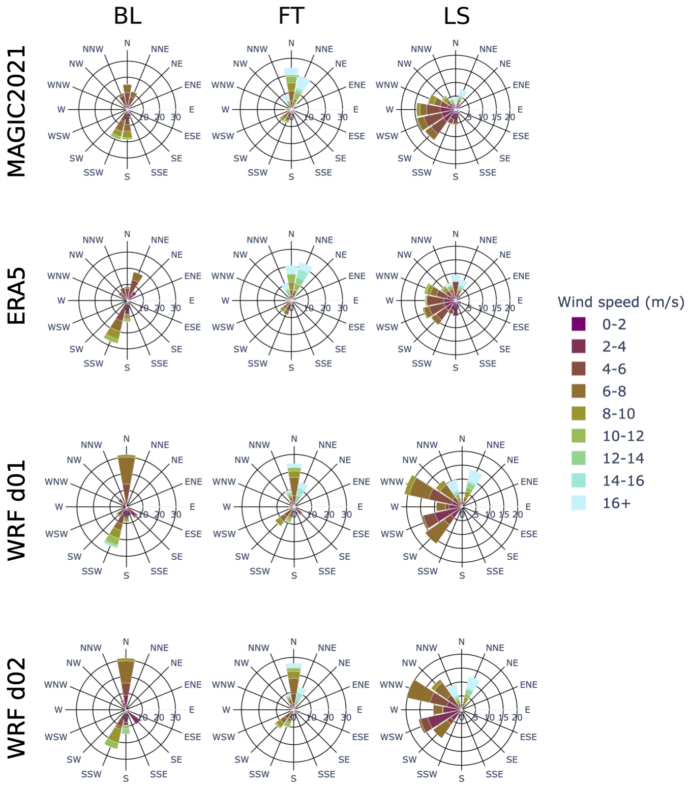
Figure 2 Wind rose plots for MAGIC2021 observations as well as ERA5 and WRF simulations. The radial axis gives the proportion (in %) of wind coming from a given direction given by the angular axis. Coloured bins represent the share of speed ranges shown in the legend associated with each direction. Rows correspond to data products MAGIC2021 observations, ERA5, WRF d01 and WRF d02. Columns correspond to atmospheric layers: Boundary Layer (BL), Free Troposphere (FT) and Lower Stratosphere (LS), described in Sect. 2.3.2.

3 Weather data comparison: Results & Discussion

3.1 Horizontal wind

Relatively high noise was observed in vertical wind measurements from aircrafts and radiosoundings, particularly when compared to the low magnitudes of the measured values. Moreover, several issues in the radiosounding data, such as unphysical steps in the recorded values, led us to exclude vertical wind data from our comparisons.

Figure 2 shows that both ERA5 and WRF manage to generally capture the observed dominant wind directions. For example, models and observations agree on a contribution superior to 20 % from notherly winds in the free troposphere. In the BL, observed winds are divided in 5 northerly and southerly main components, which all contribute less than 20 % of the sampled winds. ERA5 reproduces this distribution well, with multiple wind directions involved in low proportions while WRF overrepresents contributions from the main wind components (more than 30 % of northerly winds in the BL). This pattern is also observed in the LS and to a lesser extent in the FT.

Overall, ERA5 performs better in reproducing observed wind speed distributions, particularly in the mid-troposphere, and provides a more balanced representation of secondary wind directions at higher altitudes. WRF, on the other hand, tends to overrepresent dominant wind components while underrepresenting secondary contributions, with consistent patterns across its two domains. We now look at the statistical performance of these models in terms of wind speed and direction separately.

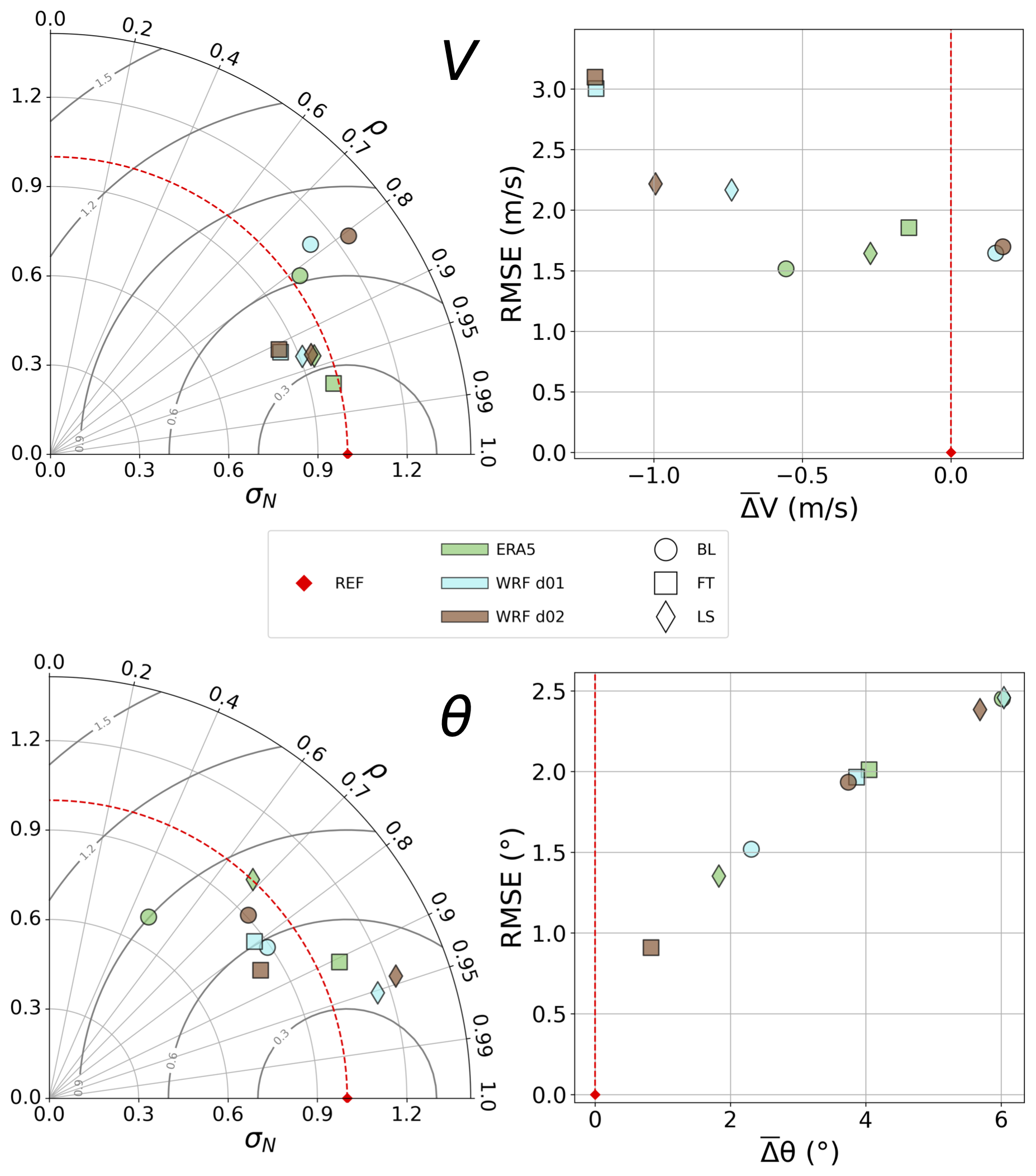
Figure 3 Comparison between simulated and observed wind speed V (top) and direction θ (bottom) with Taylor (left) and bias ($\stackrel{\mathrm{‾}}{\mathrm{\Delta }}$) versus RMSE (right) diagrams. The radial axis of Taylor diagrams represents the normalised standard deviation of modelled wind speed/direction. The angular axis represents correlation between modelled and observed wind speed/direction. Centred RMSE is represented by the radial distance from the reference point. RMSE and bias are computed subtracting observed quantities to simulated quantities.

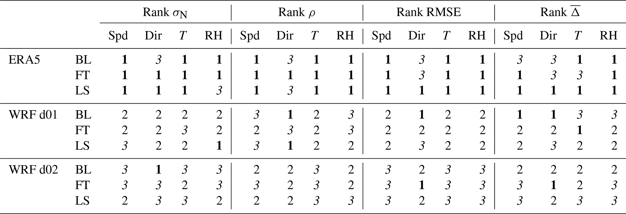
ERA5 generally outperformed WRF in wind speed metrics across the three atmospheric layers, as shown in Fig. 3. It ranked first in normalized standard deviation (σ_N) and RMSE for all layers, as well as in correlation (ρ) for the BL and FT. Specifically, ERA5 achieved a top rank in 75 % of wind speed metrics (9 out of 12, Table 3), compared to WRF d01 (16.7 %) and WRF d02 (8.3 %). For example, in the BL, ERA5 ranked first in σ_N, ρ, and RMSE, though it ranked third in bias ($\stackrel{\mathrm{‾}}{\mathrm{\Delta }}$), where WRF d01 performed best. Similarly, in the FT, ERA5 maintained its top position across all wind speed metrics except for $\stackrel{\mathrm{‾}}{\mathrm{\Delta }}$, where WRF d01 ranked first. In the LS, ERA5 continued to rank first in σ_N, RMSE, and $\stackrel{\mathrm{‾}}{\mathrm{\Delta }}$ but fell short in ρ, where WRF d01 and d02 performed better. These results highlight ERA5's consistent strength in reproducing observed wind speeds in all metrics.

For wind direction, as illustrated in Fig. 3, ERA5 and WRF showed more mixed performance. While ERA5 ranked first for some metrics in the FT and LS, WRF d01 performed better especially in the BL and LS, achieving the highest correlation (ρ) and lowest RMSE in both layers. In the BL, WRF d01 also demonstrated strong performance in other metrics, ranking first in ρ and $\stackrel{\mathrm{‾}}{\mathrm{\Delta }}$. Notably, WRF d01 outperformed the finer domain (d02) in 75 % of wind direction rankings (9 out of 12, Table 3), indicating that the coarser domain was often better suited for capturing wind direction variability and error. ERA5, on the other hand, exhibited varying performance across layers, with error metrics $\stackrel{\mathrm{‾}}{\mathrm{\Delta }}$ and RMSE rank changing with altitude (e.g. third in $\stackrel{\mathrm{‾}}{\mathrm{\Delta }}$ & RMSE in the BL and FT but first in the LS).

Overall, ERA5 exhibited superior performance in wind speed metrics across most layers, while WRF d01 showed stronger results for wind direction, particularly in the BL and LS. The relative performance of each model is summarised in Table 3. The table ranks each model against the other 2 for each physical quantity, statistical metric and atmospheric layer studied. A colour code is also given as a visual aid (green for position 1, yellow for position 2 and red for position 3). Our model assessment can then be quantified by computing the average rank of each model over all atmospheric layers and statistical metrics. ERA5 had an average rank of 1.17 in terms of wind speed, in contrast to WRF d01 (2.08) and WRF d02 (2.75). For wind direction however, both WRF d01 and d02 outperformed ERA5, with the same average rank of 1.92, compared to 2.17 for ERA5.

3.2 Temperature

Figure 4 shows temperature profiles on the upper part of the figure and temperature bias ($\stackrel{\mathrm{‾}}{\mathrm{\Delta }}$) profiles on the lower part. Here the MAGIC2021 dataset is compared to ERA5, WRF d01 and WRF d02. Bias is computed such that a positive $\stackrel{\mathrm{‾}}{\mathrm{\Delta }}T$ means that modelled temperature was superior to observations on average over all MAGIC2021 measurements in the particular bin considered. The lower-most part of the left profiles, which compare temperatures above P=800 hPa, shows a negative bias of ∼3 °C for all three models. Further investigation of model performance against each instrument separately shows that this bias was only present against AirCore data, while no significant bias was observed with other instruments, which suggests that there could have been an issue with AirCore data near the surface. In the middle section ($\mathrm{800}>P>\mathrm{300}$ hPa), models and observations follow consistently the negative vertical gradient, with ERA5 better capturing profile features, which is allowed by its better vertical resolution. Finally, in the lowest pressure levels, a good agreement between ERA5, WRF and MAGIC2021 T was found, but with more variation around $\stackrel{\mathrm{‾}}{\mathrm{\Delta }}T=\mathrm{0}$ for WRF. WRF values cannot be compared to weather balloon data in the LS above P≈50 hPa as this was set as the upper limit of the model domain. Overall, modelled temperatures reproduce well the temperatures measured during the campaign, with a mean bias consistently inferior to 2° C across all layers.

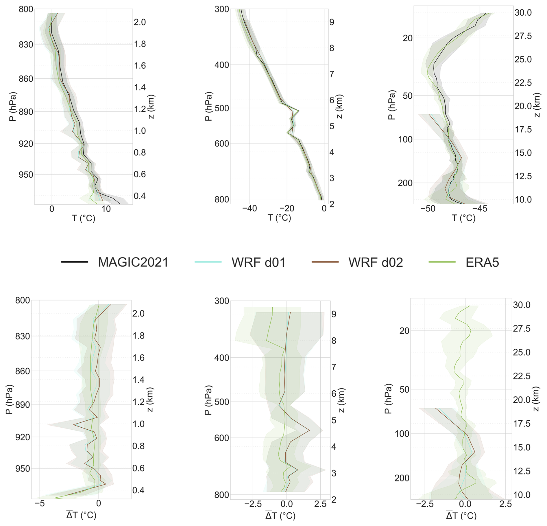
Figure 4 Vertical temperature intercomparison between MAGIC2021 data and weather models. Observational data includes MAGIC2021 data from weather balloons, ATR42 and Cessna aircraft and was binned to fit model grids. Profiles are divided in three blocks (P>800, $\mathrm{300}<P<\mathrm{800}$ and P<300 hPa) which allow to illustrate results from our analysis layers (BL, FT and LS). Shaded areas represent the 1σ deviation from the mean temperature or temperature bias profiles, computed from binned data. Top: Mean temperature profiles computed accross all flights from MAGIC2021 platforms (black) plotted with mean interpolated temperature profiles from models corresponding to platform trajectories. Bottom: Bias profiles in the same pressure ranges. Bias is computed as the mean difference between interpolated model quantities and measured physical quantities over each bin.

Figure 6 shows the statistical intercomparison with all models, metrics and atmospheric layers for both temperature and humidity (RH), the top panel focusing on temperature. It can be seen that all models performed very well in every layer, being all close to σ_N=1 and correlating very well with observations (ρ≥0.8). In terms of RMSE and $\stackrel{\mathrm{‾}}{\mathrm{\Delta }}$, models also perform well, with RMSE <2 and $\stackrel{\mathrm{‾}}{\mathrm{\Delta }}<\mathrm{1}$ °C in all layers. Models generally reproduce temperature best in the FT, followed by the LS, and then the BL across most statistical categories.

Table 3 shows that ERA5 performed better than both WRF domains in most statistical categories and layers in terms of temperature as well, with an average rank of 1.17 for ERA5 versus an average rank >2 for WRF. Overall, WRF d01 and d02 showed closely similar performance in all layers, with WRF d01 slightly but consistently outperforming d02 in most statistical metrics and layers (average rank of 2.08 for WRF d01 and 2.75 for d02).

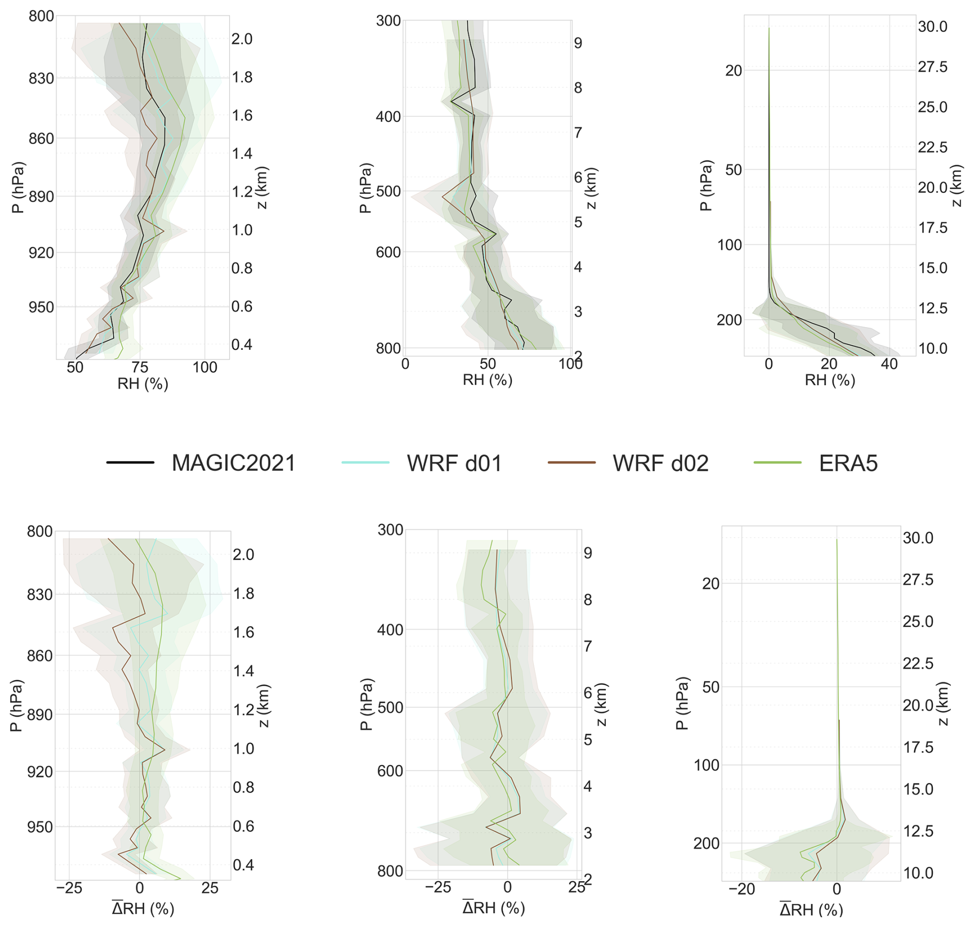
Figure 5 Vertical relative humidity intercomparison between MAGIC2021 data and weather models. Observational data includes MAGIC2021 data from weather balloons, ATR42 and Cessna aircraft and was binned to fit model grids. Profiles are divided in three blocks (P>800, $\mathrm{300}<P<\mathrm{800}$ and P<300 hPa) which allow to illustrate results from our analysis layers (BL, FT, LS). Shaded areas represent the 1σ deviation from the mean RH or RH bias profiles, computed from binned data. Top: Mean RH profiles computed accross all flights from MAGIC2021 platforms (black) plotted with mean interpolated RH profiles from models corresponding to platform trajectories. Bottom: Bias profiles in the same pressure ranges. Bias is computed as the mean difference between interpolated model quantities and measured physical quantities over each bin.

3.3 Humidity

As for temperature, relative humidity profiles for ERA5, WRF d01 and WRF d02 are shown on Fig. 5. The top panel shows the mean RH profile observed during MAGIC2021 and the corresponding mean interpolated profiles for each model. The bottom panel shows the corresponding bias profiles. The left handside profiles show that humidity increased with height on average from the surface up to about z=1.5 km, which was well captured by all models. The bias profiles also suggest RH_ERA5> RH_WRFd01> RH_WRFd02 throughout the highest pressure levels. In the middle block, the models also captured the decrease in RH with height well; however, the previously observed tendency of higher RH values in ERA5 compared to WRF d01 and WRF d02, is no longer there. At lower pressure levels, RH strongly decreased with height and reaches ∼ 0 % just below z=15 km which was captured by all models but with an underestimation of the observed RH values between 10 and 12 km.

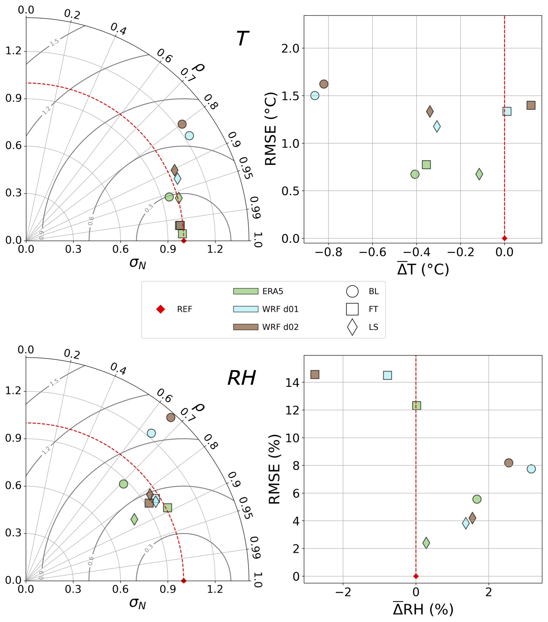
Figure 6 Comparison between simulated and observed temperature (top) and relative humidity (bottom) with Taylor (left) and bias ($\stackrel{\mathrm{‾}}{\mathrm{\Delta }}$) versus RMSE (right) diagrams. The radial axis of Taylor diagrams represents the normalised standard deviation of modelled $T/$ RH. The angular axis represents correlation between modelled and observed $T/$ RH. Centred RMSE is represented by the radial distance from the reference point. RMSE and bias are computed subtracting observed quantities to simulated quantities.

The bottom panel of Fig. 6 shows the full statistical intercomparison with 4 metrics and 3 layers (BL, FT and LS) for relative humidity. Models correlated best with MAGIC2021 measurements in the LS and FT, and less in the BL. Variability was also generally better represented in the FT and LS than in the BL, with σ_N being closer to 1. Model performance was good overall, but showing worst numbers than for temperature. σ_N values ranged from 0.75 to 1.4 and ρ went from just under 0.65 in the BL to ∼ 0.9 in the FT. ERA5 performed once again better both in terms of correlation and σ_N than WRF in all layers. In terms of RMSE, RH was least well represented in the FT, where a RMSE >12 % was observed for all models. The BL was where bias was highest, at around 2 % on average, depending on the model. For WRF, the bias observed in the BL was opposite to the bias in the FT. All models showed their best performance in terms of RMSE and bias in the LS, due to the low values of RH at this altitude. ERA5 showed consistently better performance in terms of RMSE and bias whilst WRF d01 and d02 showed better σ_N performance in the FT and LS respectively.

These results are summarised in Table 3 where ERA5 gets the first position in all layers and metrics, except for σ_N in the LS, where WRF d01 and d02 did not simulate RH up to the same height as ERA5, which could explain the better performance of WRF in that layer. The overall performance of WRF d01 and d02 was similar, but WRF d01 did outperform d02 in terms of average rank (2.17 for d01 versus 2.67 for d02).

Table 3 Simulation rank depending on the meteorological quantity assessed for the three atmospheric layers and the four statistical metrics considered in the study. Spd refers to wind speed, Dir to wind direction, T to temperature and RH to relative humidity comparisons. Best performance (rank 1) shown in bold, poorest performance (rank 3) in italics.

3.4 Conclusions on weather data comparison

The good performance of both ERA5 and WRF in terms of horizontal wind speed and direction was not surprising as they are widely used and well validated models. ERA5 speed scores were better than both WRF d01 and d02, and direction scores were about equivalent even though both WRF domain slightly outperformed ERA5. Over all physical quantities, atmospheric layers and statistical metrics, ERA5 obtained an average rank of 1.42, WRF d01 a rank of 2.06 and WRF d02 a rank of 2.52. The fact that ERA5 is a reanalysis product could explain its better performance, as it benefits from data assimilation unlike WRF. WRF could be expected to perform better than ERA5 in the boundary layer, given its fine resolution and use of an advanced PBL scheme to model turbulence. In particular, $\stackrel{\mathrm{‾}}{\mathrm{\Delta }}$ should get better with higher resolution, however noise related metrics could be expected to get worse as higher resolution implies more potential noise. We indeed found lower $\stackrel{\mathrm{‾}}{\mathrm{\Delta }}$ in both wind speed and direction for WRF over ERA5 in the BL. However, performance did not improve significantly between d01 and d02, with d01 even outperforming d02 in bias for wind direction in the BL. Metrics other than $\stackrel{\mathrm{‾}}{\mathrm{\Delta }}$ are all influenced by noise even though RMSE and σ_N do not depend solely on it. Thus we use CRMSE, represented by radial distance from the reference point in Taylor diagrams, to assess model noise performance. We find that WRF d01 and d02 have slightly higher CRMSE than ERA5 in the BL & FT for wind speed but not for direction which only partially confirms our hypothesis. Mass et al. (2002); Gómez-Navarro et al. (2015) explained in more detail how higer resolution in simulations can lead to worse performance in objective statistical assessments. They demonstrated that, whilst simulations with finer resolution could enhance the representation of physical processes compared to coarser simulations, they are more significantly influenced by timing and spatial inaccuracies. This explains the better results obtained with ERA5, compared to WRF d01 and WRF d02, also highlighting the challenges involved in validating high-resolution models. It also underscores that employing a range of statistical measures enables more robust evaluations of model performance. WRF outputs can be improved by nudging, which involves adjusting model estimates using observations or reanalysis products, to help regional simulations fit observations better (Bullock et al., 2014), but nudging was not utilised in the WRF runs analysed here, to specifically compare WRF physics to ERA5. Data assimilation could be implemented in our simulations using WRFDA, the data assimilation system included in WRF (Pattanayak and Mohanty, 2018) in order to directly compare model physics, as well as quantifying the impact of data assimilation on simulations in that region.

Assessment of temperature was also characterised by an overall very good performance from all simulations ($\stackrel{\mathrm{‾}}{\mathrm{\Delta }}<\mathrm{1}$ K in all layers). Temperatures from weather balloons appear to be slightly biased (by about 2 K) in the BL. This could be due to a lack of corrections of temperatures measured in the boundary layer by the M20. Further checks did not find any correlation between wind speeds and $\stackrel{\mathrm{‾}}{\mathrm{\Delta }}T$ as measured by the instrument, so no physical disturbance appeared to have been interferring with measurements. This was unexpected as calibration was performed prior to balloon release on the ground, in that surface layer. It is worth noting that consistent $\stackrel{\mathrm{‾}}{\mathrm{\Delta }}>\mathrm{0}$ was only found in some flights (002, 003, 004 on 21/08 and 22/08) that had $\stackrel{\mathrm{‾}}{\mathrm{\Delta }}>\mathrm{1}$ K in the BL, the other half of the flights not showing this characteristic. Investigating those particular flights in more detail appears necessary to understand the origin of our findings.

Overall, WRF simulations were close to both ERA5 and MAGIC2021 data in terms of performance, which gives confidence in the ability of the model to simulate the atmosphere in our region of interest.

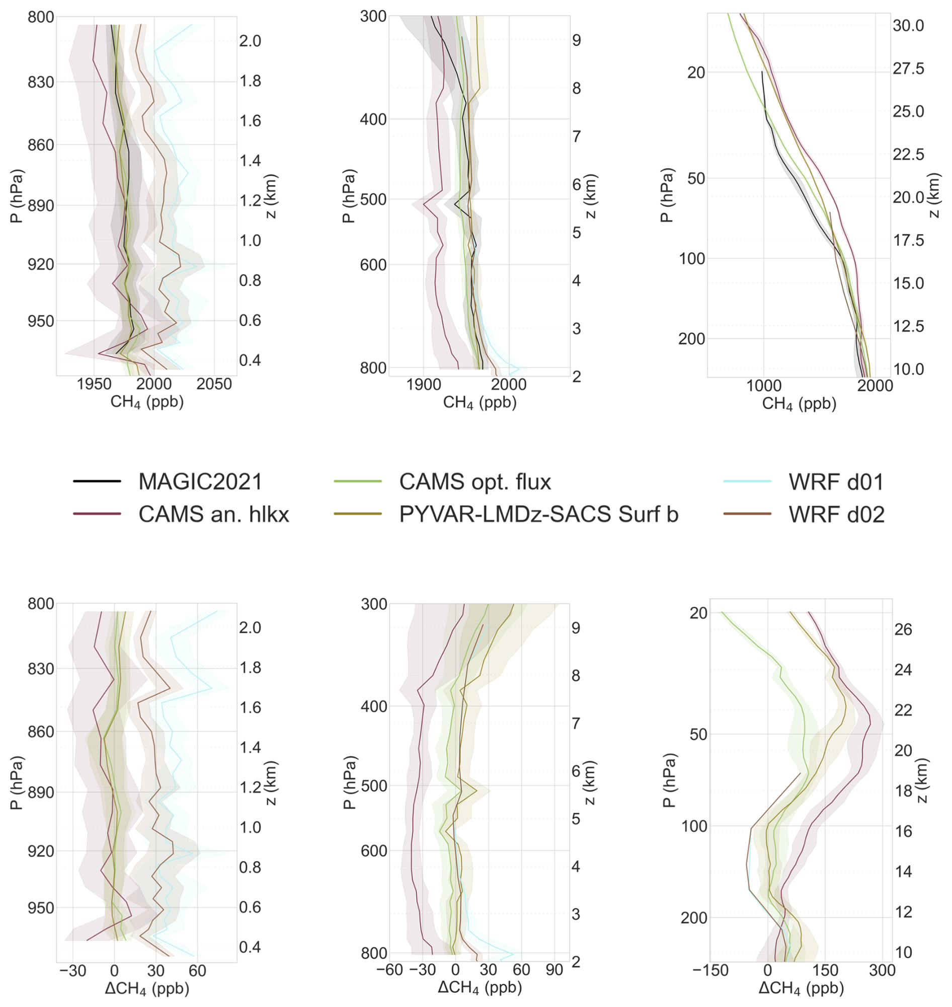
Figure 7 Vertical methane intercomparison between MAGIC2021 data and chemistry-transport models. Observational data include MAGIC2021 samples from AirCores, ATR42 and Cessna aircraft and were binned to fit model grids. Profiles are divided in three blocks (P>800, $\mathrm{300}<P<\mathrm{800}$ and P<300 hPa) which allow to illustrate results from our analysis layers (BL, FT, LS). Shaded areas represent the 1σ deviation from the mean CH₄ or CH₄ bias profiles, computed from binned data. Top: Mean CH₄ profiles computed accross all flights from MAGIC2021 platforms (black) plotted with mean interpolated CH₄ profiles from models corresponding to platform trajectories. Bottom: Bias profiles in the same pressure ranges. Bias is computed as the mean difference between interpolated model quantities and measured physical quantities over each bin.

4 Assessment of CH₄ simulations

4.1 Comparison between modelled and observed CH₄ profiles

CH₄ mixing ratio profiles and CH₄ bias profiles ($\stackrel{\mathrm{‾}}{\mathrm{\Delta }}$CH₄) computed for several models versus MAGIC2021 data are shown on Fig. 7. The left profiles show comparisons for P>800 hPa, the middle profiles $\mathrm{800}>P>\mathrm{300}$ hPa and the right profiles for P<300 hPa. Only PLS Surf b results are shown from the 6 different model products, as it performed best overall (details shown in Fig. 8, Table 4 and Fig. A4). In the P>800 hPa profiles, CH₄ mixing ratios from global models were close to or smaller than CH₄ from MAGIC2021 measurements, while regional models simulated higher CH₄ content than in-situ measurements. This was observed with all three platforms (see Fig. A3 for details), with specifically PLS Surf b and CAMS v21r1 showing the best fit to the observed CH₄ mixing ratios while CAMS hlkx CH₄ mixing ratios were negatively biased. Regional simulations from WRF-Chem, mainly influenced by surface emissions in the BL, produced mixing ratios higher than MAGIC2021 measurements (of ∼20–100 ppb in d01 and ∼20–50 ppb in d02).

In the $\mathrm{800}>P>\mathrm{300}$ hPa profiles, CAMS hlkx mixing ratios were consistently below MAGIC2021 measurements, by about 25–50 ppb. PLS Surf b and CAMS v21r1 simulations performed well again with $\stackrel{\mathrm{‾}}{\mathrm{\Delta }}$CH₄ close to 0 throughout all levels. Regional model biases decreased significantly with altitude (800–300 hPa), reducing the gap between d01 and d02 showing similar bias as CAMS v21r1 and PLS Surf b.

In the LS, CAMS hlkx transitioned from a negative bias in the FT to a strong positive bias exceeding 200 ppb at P∼50 hPa. PLS Surf b, CAMS v21r1, and WRF-Chem displayed more complex bias profiles in this region. They were characterised by a first peak in bias (50–100 ppb) near 250 hPa, followed by a decrease to −50–0 ppb between 175 and 100 hPa, and then a second increase to 100–200 ppb at pressures below 100 hPa. In the FT and LS, WRF-Chem mixing ratios closely followed CAMS v21r1 (product that was used as boundary conditions). A deviation from this behaviour was observed in the LS above the first peak in bias at approximately 300 hPa, likely due to transport differences between WRF-Chem and TM5 (the transport model used in CAMS v21r1).

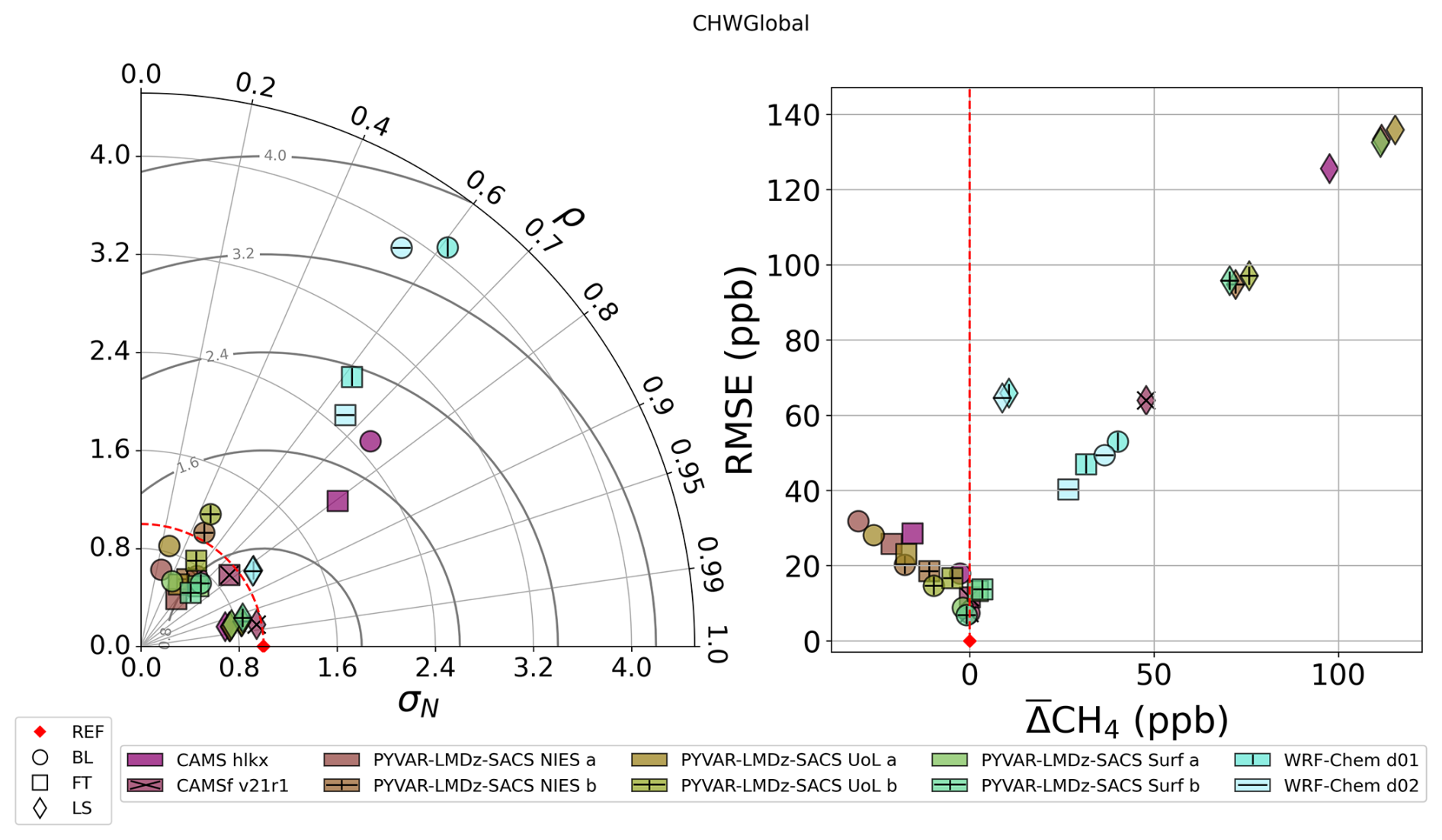
Figure 8 Left: Taylor diagram for CH₄ comparisons between MAGIC2021 observations and ERA5 model. The radial axis represents the normalised standard deviation of the modelled CH₄. The angular axis represents the correlation between modelled and observed CH₄. The centred RMSE is represented by the radial distance from the reference point. Right: RMSE against bias ($\stackrel{\mathrm{‾}}{\mathrm{\Delta }}$CH₄) computed from MAGIC2021 observations and modelled CH₄. RMSE and bias are computed subtracting observed quantities to simulated quantities.

Figure 8 shows results from the comparison between MAGIC2021 CH₄ measurements and models according to the four statistical metrics and the 3 atmospheric layers used previously. In the BL, most ($\mathrm{5}/\mathrm{8}$) global simulations underestimated the variability of atmospheric CH₄ content (σ_N<1). On the contrary, regional simulations significantly overestimated this variability with σ_N>3 for both d01 and d02 domains. Correlation between model products and MAGIC2021 measurements was also found to be low in the BL, no simulations exceeding ρ=0.8, with some reaching values below ρ=0.4 (PLS NIES a and PLS UoL a). In terms of bias and RMSE, global models had better performance in the BL when compared to regional simulation products, particularly PLS Surf a and b and CAMS v21r1 which all had RMSE <10 ppb and absolute values of bias ≤1 ppb. Whereas global simulations all displayed a negative bias, both WRF-Chem domains overestimated methane content in the BL, which corresponds to what was observed in the profiles of Fig. 7.

The FT was also characterised by an underestimation of variability by global models with most ($\mathrm{7}/\mathrm{8}$) having σ_N<1. Regional simulations along with CAMS hlkx once again overestimated variability in that layer, with $\mathrm{1.7}\le {\mathit{\sigma }}_{\mathrm{N}}\le \mathrm{3.5}$. Correlation performance was slightly better than in the BL, with most ($\mathrm{6}/\mathrm{10}$) models showing ρ>0.6. RMSE and bias performance was also better in the FT than in the BL, with the notable exception of CAMS hlkx that displayed a negative bias of ∼30 ppb as was seen in the profiles of Fig. 7.

In the LS, all global models had a similar performance in terms of correlation, achieving the highest values out of the three analysis layers ($\mathrm{0.95}\le \mathit{\rho }\le \mathrm{0.99}$). Regional simulations showed a lower correlation with MAGIC2021 measurements, with ρ∼0.85 for both domains. Variability was underestimated by all global models in the LS, with $\mathrm{0.68}\le {\mathit{\sigma }}_{\mathrm{N}}\le \mathrm{0.95}$ while both domains of the regional simulations slightly overestimated variabillity. Positive biases were observed for all simulations in the LS, more particularly for global models which showed $\mathrm{43}<\stackrel{\mathrm{‾}}{\mathrm{\Delta }}<\mathrm{103}$ ppb. Regional simulations managed to produce a lower bias, with $\stackrel{\mathrm{‾}}{\mathrm{\Delta }}<\mathrm{10}$ ppb for both WRF-Chem d01 and d02. In terms of RMSE, CAMS v21r1 performed best among all global models with RMSE ∼ 60 ppb, which aligned with both WRF-Chem domains. For PLS products, the “advanced” physics configuration (b) also showed better results than the “classic” physics scheme (a), both in terms of RMSE and bias.

In conclusion, the evaluation of model simulations against MAGIC2021 CH₄ measurements revealed distinct performance patterns across atmospheric layers. In the BL, global simulations underestimated CH₄ variability and showed lower bias and RMSE compared to regional simulations, which overestimated both variability and CH₄ content. In the FT, regional simulations better represented variability, but correlation remained low for most models, with improved RMSE and bias relative to the BL. In the LS, global models achieved high correlation with MAGIC2021 measurements but displayed large positive biases, while regional simulations provided lower biases and comparable RMSE performance.

4.2 Discussion of CH₄ comparisons

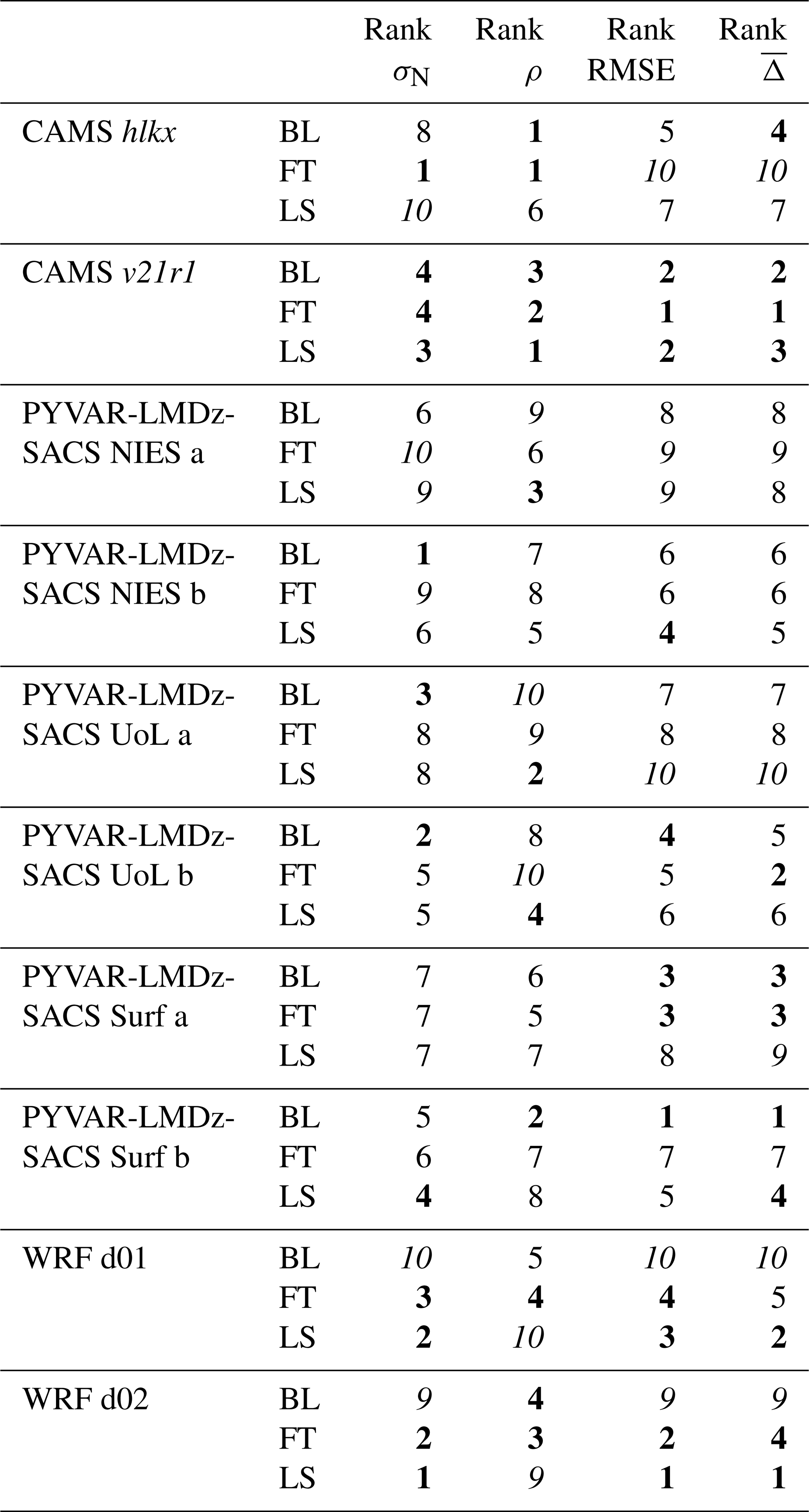
Table 4 shows a comparative assessment of the simulated atmospheric CH₄ content by the 10 modelling frameworks against MAGIC2021 observational data. Consistently with our previous discussion, CAMS v21r1 shows the best overall performance, in most metrics and layers, having an average rank of 1.75. The table also allows to rank the PLS inversions ensemble according to their average rank in all layers and metrics used (shown in parenthesis): 1. Surf b (3.83), 2. Surf a (4.92), 3. UoL b (5.08), 4. NIES b (5.25), 5. UoL a (7), 6. NIES a (7.58). Thus the worst performing simulations were PLS NIES a and PLS UoL a, with PLS Surf a also performing worst than PLS Surf b. This indicates that updating from the “classic” to “advanced” physics scheme makes a more important difference than a change in observational constraint for these simulations.

Table 4 CH₄ simulations ranking for the three atmospheric layers and the four statistical metrics considered in the study.Best performance (1–4) shown in bold, poorest performance (9–10) in italics.

We first start by discussing BL positive biases observed in regional WRF-Chem CH₄ products. WRF-Chem d01 and d02 results presented in Figs. 7 and 8 are an average over eleven different products for each of d01 and d02 domains. As such, individual products had differing performance scores in the four metrics of the study. To investigate results from regional simulations in more depth, we show results from individual WRF-Chem products in Fig. 9. This figure shows the same 4-metric assessment as in Fig. 8, but it focuses on individual WRF-Chem simulations, which differ by their input CH₄ emissions from wetlands. WRF-Chem d02 products performed better than d01 in most layers and statistical metrics (ρ performance was inventory dependent and very close between d01 and d02). For all products, the assessment showed that mixing ratios were positively biased in the BL and the FT, with a stronger bias in the BL. Most global model products showed a negative bias in the BL ($\mathrm{7}/\mathrm{8}$) and an underestimate of variability ($\mathrm{5}/\mathrm{8}$), contrary to WRF-Chem mixing ratios which showed both a positive bias and an overestimate of variability. This is consistent with an understimate/overstimate of surface emissions as weak sources would both lead to a negative $\stackrel{\mathrm{‾}}{\mathrm{\Delta }}$ and a decrease in variability, whilst overestimated surface emissions would lead to both a positive $\stackrel{\mathrm{‾}}{\mathrm{\Delta }}$ and an overstimated variability of boundary layer mixing ratios. This could also be explained by vertical transport issues (e.g. an underestimation of the BL height) in WRF, which could have participated in producing higher CH₄ mixing ratios in the BL. However, the consistency between WRF-Chem simulations and MAGIC2021 data in the FT implies that the vertical transport representation in WRF-Chem was accurate, thus indicating that CH₄ overestimates in the BL from WRF-Chem products was more likely stemming from wetland emission models. This was further confirmed by the relative scale of input emissions shown in Table 1, which correlates with the relative scale of CH₄ overestimates in the BL shown in Fig. 9. Moreover, the particular WRF-Chem set-up used in this study has been used in previous studies without showing any issues with BL or FT transport (Lauvaux et al., 2012, 2016). Thus we deduced that inventories overestimated the magnitude of wetland emissions (which could also lead to overestimating flux variability).

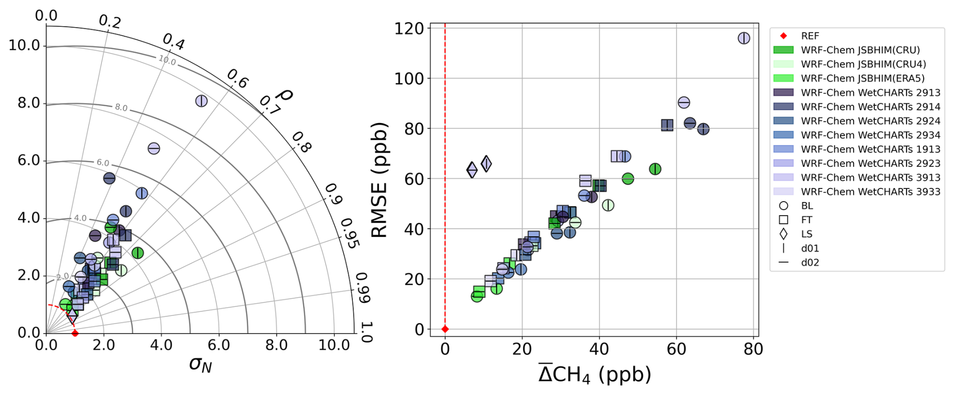
Figure 9 Statistical assessment of individual WRF-Chem simulations against MAGIC2021 measurements Left: Taylor diagram for CH₄ comparison between MAGIC2021 observations and WRF-Chem. The radial axis represents the normalised standard deviation of the modelled CH₄ , whilst angular position represents correlation between modelled and observed CH₄ . Centred RMSE is represented by the radial distance from the reference point. Right: RMSE against bias ($\stackrel{\mathrm{‾}}{\mathrm{\Delta }}$CH₄) computed from MAGIC2021 observations and modelled CH₄. RMSE and bias are computed subtracting observed quantities to simulated quantities.

These results first showed that low emissions are needed to match observations when looking at averages over the whole MAGIC2021 dataset. Wetland methane releases are typically not homogeneously distributed and continuous in space and time (Rinne et al., 2018; Waletzko and Mitsch, 2014) which makes them hard to fully encompass in inventories. This is reinforced by the fact that not only WetCHARTs monthly averaged emissions led to such overstimates, but also JSB-HIM products which have a daily time resolution as well as a higher spatial resolution and more complex underlying emission processes. Thus, a true improvement in the representation of wetland emissions would require sub-daily and sub-kilometer resolution as there is no clear difference in performance between monthly/0.5° and daily/0.1° resolution products.

This issue with wetland emission models could be investigated further by combining MAGIC2021 BL observations with high resolution WRF-Chem simulations and other modelling techniques such as Lagrangian particle dispersion modelling.

The FT negative bias found between CAMS hlkx and MAGIC2021 observations is similar to previous findings by Membrive et al. (2017) where simulations similar to CAMS hlkx (C-IFS forecast) were compared to a high resolution profile from an AirCore launch in Canada during the StratoScience campaign (CNES – August 2014). More precisely, the instrument (AirCore-HR) was deployed on a stratospheric balloon flight near Timmins, ON. (48.6° N). This study compares well with ours because similar CH₄ sources can be found near both locations, and data was also collected in August. Membrive et al. (2017) found $\stackrel{\mathrm{‾}}{\mathrm{\Delta }}=-\mathrm{24}$ ppb when comparing AirCore measurements to the C-IFS forecast. We find an overall tropospheric $\stackrel{\mathrm{‾}}{\mathrm{\Delta }}$ of $-\mathrm{14.7}\pm \mathrm{16.6}$ ppb when comparing MAGIC2021 versus CAMS hlkx, which is a comparable result. Further conclusions cannot be drawn from comparing these two studies alone, but this feature is also consistently found when comparing AirCore profiles from AirCore networks (AirCore-Fr, Crevoisier et al., 2023, NOAA; Koffi and Bergamaschi, 2018) with CAMS forecast and analysis products. This suggests the presence of a systematic CH₄ bias in the FT in CAMS forecast and analysis products.

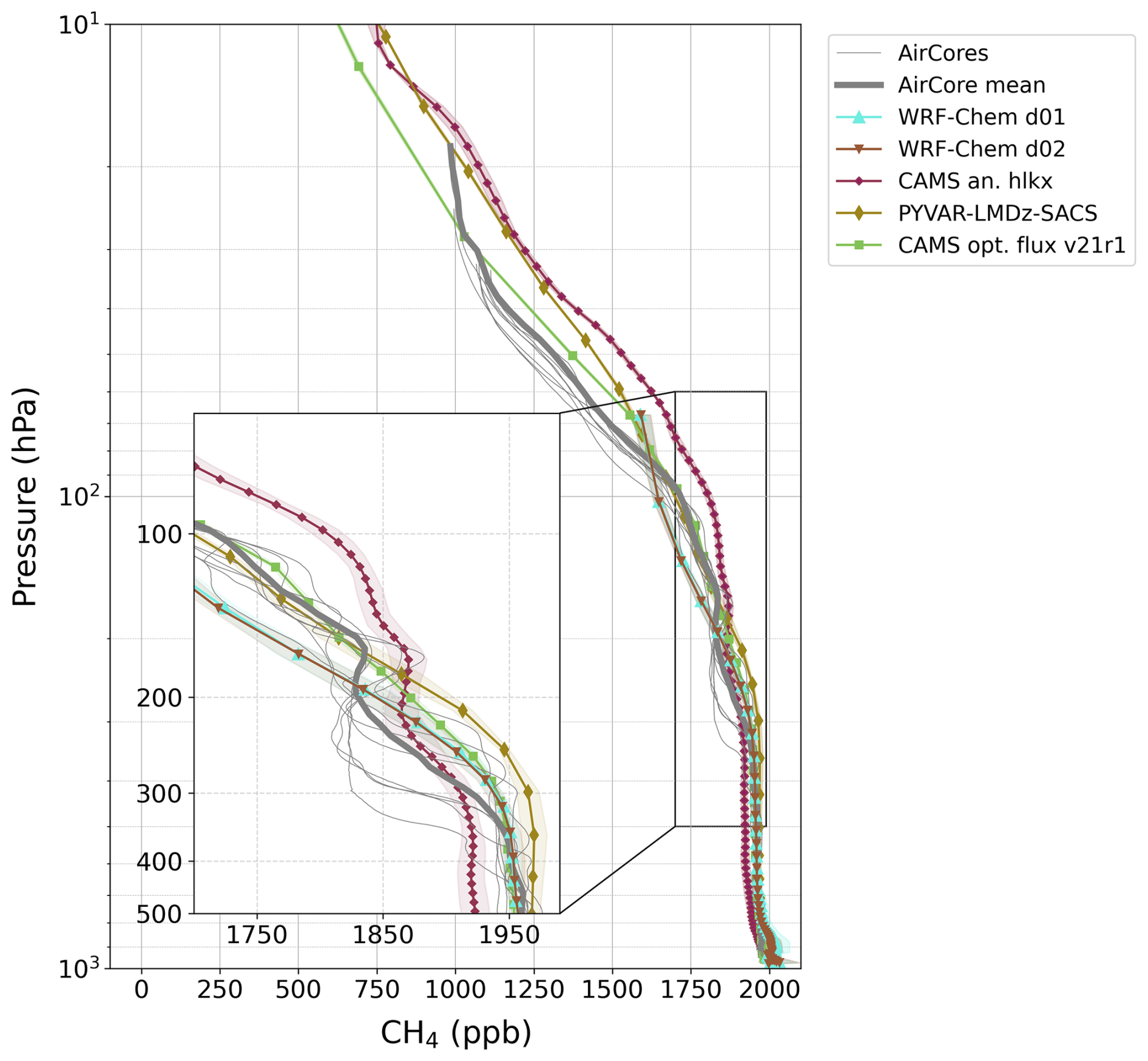
Figure 10 CH₄ profiles from MAGIC2021 AirCores (symbol-free lines) plotted with modelled CH₄ profiles (lines with symbols) against pressure. Displayed modelled profiles are averaged over all interpolated profiles for each model and the coloured area represents the 1σ deviation from the mean. From the PLS ensemble, only the best performing product (Surf b) is shown.

Whilst a significant tropospheric bias was only found between CAMS hlkx and MAGIC2021 measurements, LS analysis highlighted the presence of a strong positive bias for all models (cf. Fig. 7). This is particularly important as a stratospheric bias in CH₄ levels affects the performance of models at reproducing the dry-air column-averaged mixing ratio of methane (XCH₄), which has to be accurately reproduced in order to leverage satellite observations to measure surface emissions of CH₄ (Ostler et al., 2016). To investigate this further, we drew Fig. 10 which shows all MAGIC2021 AirCore profiles plotted along with mean and spread of corresponding interpolated model profiles. Measured CH₄ profiles show three distinct phases in the LS. The bottom of the layer is characterised by a first strong gradient, typically from P=400–300 to P=200 hPa, which takes CH₄ mixing ratios from their tropospheric average of ∼1950 ppb to about 1810 ppb. mixing ratios then remain stable for 100 hPa or less before starting a sharp decrease again in the last layer, between P=200 and P=100 hPa. This overall structure is in reality more complex when looking at individual profiles and highlights the stratification of the atmosphere at these altitudes.

Membrive et al. (2017) attribute LS $\stackrel{\mathrm{‾}}{\mathrm{\Delta }}>\mathrm{0}$ in C-IFS simulations similar to CAMS hlkx to an understimation of the CH₄ stratospheric gradient, which then becomes too steep higher in the stratosphere (Verma et al., 2017). We indeed observe a growing positive model bias in the LS between 12 and 20 km (or P=200 to P=45 hPa) on the bottom right panel of Fig. 7). This bias then decreases and becomes positive for some simulations higher in the stratosphere. These results were found for all global models including CAMS hlkx, which is a similar product to the one assessed in Verma et al. (2017) and Membrive et al. (2017). However, the 4-metric assessment performed on models showed that correlation between MAGIC2021 measurements and all simulations had high correlation in the LS, which indicates a good reproduction of CH₄ gradients by the models within that layer. These results suggest that the CH₄ stratospheric biases found here and in the literature have a complex origin. Fig. 10, showed that CH₄ values from AirCores started to decrease more strongly at lower altitudes than in models, meaning that the reduction in CH₄ mixing ratios in the upper troposphere due to interaction with OH radicals could be starting higher in models than in reality. Patra et al. (2011) compared several simulations of CH₄ and CH₃CCl₃, including some made with a set-up similar to the PLS model, and showed that models differed in their bias with the same OH field, indicating that other factors than the reaction between CH₄ and tropospheric OH, such as other chemical reactions or transport, are involved. Among the other important chemical reactions, CH₄ is also depleted by chlorine (Cl) in both the troposphere and stratosphere. Thanwerdas et al. (2022) simulated the Cl sink in a CTM also using LMDz for transport and found similar highly positive model biases near the tropopause, on which changes in the Cl field had little to no effect. Together, these results indicate that transport issues in the assessed models are more likely to explain the observed biases than factors related to chemistry.

The strength of CH₄ stratospheric decay has been linked to the rate of stratosphere-troposphere exchanges (STE), which is directly influenced by the Brewer-Dobson circulation (that controls tropopause height tropopause folds) or fronts/cyclones (Holton et al., 1995; Thompson et al., 2014; Locatelli et al., 2015). Modelling STE accurately is therefore crucial to match observed CH₄ mixing ratios at these altitudes because they vary strongly over a short vertical distance depending on the chemical content of the air masses within which measurements are made. Our results regarding tropopause height in temperature profiles (Fig. 4) show that outputs from the IFS transport model (which is used in ERA5 and CAMS simulations) have good consistency with observations in the lower stratosphere, indicating that transport issues might be due to other reasons. CAMS hlkx has three to four times as many vertical levels as the other products that are compared to MAGIC2021 observations. In the LS, and especially at the tropopause, this feature makes an important difference in terms of structure complexity of profiles. As such, the CAMS hlkx bias profile does not show the positive peak of $\stackrel{\mathrm{‾}}{\mathrm{\Delta }}\sim \mathrm{50}$–100 ppb for $\mathrm{300}>P>\mathrm{200}$ hPa that inversion-optimised models (PLS, CAMS v21r1) do. This could be because it can capture a more realistic vertical structure of CH₄ depletion near the tropopause, as shown in Fig. 10.

Patra et al. (2011); Thompson et al. (2014) showed that STE were poorly modelled in a CTM set-up similar to the PLS simulations used here. This poor performance was attributed to a bad simulation of the Brewer-Dobson circulation, which was too vigorous, inducing too much stratosphere-troposphere mixing. A crucial difference between the set-up from Patra et al. (2011); Thompson et al. (2014) and ours was the number of vertical levels (19 in their set-up versus 39 in ours). Locatelli et al. (2015) have also suggested that more vertical levels would allow for a better modelling of the Brewer-Dobson circulation, notably allowing for a better computation of the tropopause height and better mixing. Their hypothesis, suggesting that a Brewer-Dobson circulation stronger in models than in reality would enhance mixing and reduce the CH₄ gradient at the tropopause fits well with our results, given that the model with the most vertical levels is able to better reproduce observed profile features. Nevertheless, this finding warrants cautious interpretation, as CAMS hlkx simulations only display mediocre performance in the lower stratosphere (LS) across our four statistical metrics. The comprehensive summary of our model assessment presented in Table 4 positions CAMS hlkx at the 10th rank for σ_N, 4th for ρ, and 7th for both $\stackrel{\mathrm{‾}}{\mathrm{\Delta }}$CH₄ and RMSE within the LS. It should be noted that CAMS hlkx represents a less refined product in relative to other models, lacking surface CH₄ emissions optimisation or data assimilation included in other CAMS products such as CAMS v21r1. Potential next steps would involve comparing LS observations with higher vertical resolution emission-optimised CH₄ simulations, thereby enabling more definitive conclusions on this matter.

While we saw that issues with individual chemical species such as OH (Patra et al., 2011) or Cl (Thanwerdas et al., 2022) could not explain the observed CH₄ LS bias by themselves, it is possible that a combination of errors in chemistry modelling could partly explain it. Thus, another possible way to improve the performance of chemistry-transport models in the LS would be to couple them with models that focus on stratospheric chemistry, such as REPROBUS (Lefèvre et al., 1994, 1998; Jourdain et al., 2008), which implement stratospheric chemistry in more detail, notably taking into account more CH₄ sink molecules, thus potentially preventing CH₄ overestimates. Comparing AirCore profiles to LMDz-Reprobus (Marchand et al., 2012) CH₄ products would shed some light on the impact of chemistry on modelled CH₄ mixing ratios in the LS.

4.3 Conclusions on CH₄ comparisons

Our model performance intercomparison highlights important differences between MAGIC2021 observations and modelled CH₄ mixing ratios, especially in the LS where all models overestimate atmospheric methane levels. CAMS hlkx analysis showed highest bias of all models in the LS and also suffered from consistent underestimation of atmospheric methane content in the FT. Inversion-optimised products showed better perfomance at every levels than CAMS hlkx. However, CAMS hlkx denser vertical grid at high altitude proved to be a certain advantage to better resolve the structure of CH₄ profiles at the tropopause. Among inversion optimised global chemistry-transport models, CAMS v21r1 showed the best performance in terms of $\stackrel{\mathrm{‾}}{\mathrm{\Delta }}$CH₄. Standard physics and surface observational constraints were found to be the best combination within the 6 PLS ensemble inversions, this version (Surf b) showing a similar level of performance as CAMS v21r1. We also find that updating the physics scheme from “classic” to “advanced” improves PLS simulations more than a change in observational constraints. Regional simulations were characterised by a strong overestimation of the BL CH₄ atmospheric content, which was not found in global simulations. This overestimation hints toward either an excess in wetland emissions from input bottom-up models or a vertical transport problem in WRF-Chem. The good correspondance between WRF-Chem simulations and MAGIC2021 data in the FT indicate that the issue probably lies with wetland emission models rather than with the vertical transport representation in WRF-Chem.

5 Conclusions

ERA5 reanalysis and WRF simulations were assessed using meteorological data from MAGIC2021. Methane in-situ measurements from MAGIC2021 were also exploited to assess atmospheric composition models: the analysis product CAMS hlkx, the inversion-optimised product CAMS v21r1, six PYVAR-LMDz-SACS (PLS) ensemble inversions and WRF-Chem regional simulations. Over the six days of MAGIC2021, meteorological data from ERA5 showed better agreement with observations than WRF on average, due to both data assimilation and lower resolution that enhance performance in such an exercise. WRF performance was however very close for all physical quantities assessed, which gives us confidence in its ability to simulate regional atmospheric physics for MAGIC2021. Among global simulations, inversion-optimised simulations of CH₄ mixing ratios performed best, especially close to the surface. CAMS v21r1 showed slightly better performance than the best product from the PLS ensemble inversions. A detailed analysis of regional simulations with WRF-Chem was performed, revealing perfomance disparities among CH₄ products. Notably, near-neutral to strongly positive biases were observed in the boundary layer, indicating a tendency of wetland emission models to overestimate CH₄ emissions, at least for the limited region and timeframe captured by the observations. CH₄ profiles were also characterised by performance discrepancies near the tropopause, where CH₄ content is depleted mainly by its reaction with OH radicals, and can also be affected by stratospheric intrusions. All models showed a delayed vertical gradient of CH₄ mixing ratios near the tropopause, leading to a positive bias in the stratosphere. Comparisons with CAMS hlkx showed that high vertical resolution allows to better capture vertical structure of CH₄ profiles in the stratosphere, with a large overestimate still. These results call for more work dedicated to improve the transport and chemistry of models in the LS, which could be done by separate stratosphere models, specialised in the task. Finally, we aknowledge that the MAGIC2021 dataset is limited in both spatial and temporal extents, limiting its ability to fully assess models. While the MAGIC2021 campaign provides valuable observations, supplementing this with additional datasets could offer a more comprehensive evaluation of model performance. This could be partly addressed by using data from other campaigns (e.g. CoMet 2.0 campaign over Canada in the summer of 2022, https://comet2arctic.de/, last access: 27 October 2025) together with data from MAGIC2021. Still the results presented here represent a rare opportunity to assess the performance of models against a large, high resolution dataset, and over an area where few measurements are usually taken, highlighting the ability of extended campaigns at high latitudes to characterise local processes. More frequent campagins could allow to extend this kind of performance assessment of global and regional models to other circumpolar regions and seasons, while also allowing a long term tracking of atmospheric composition changes in the Arctic.

Appendix A

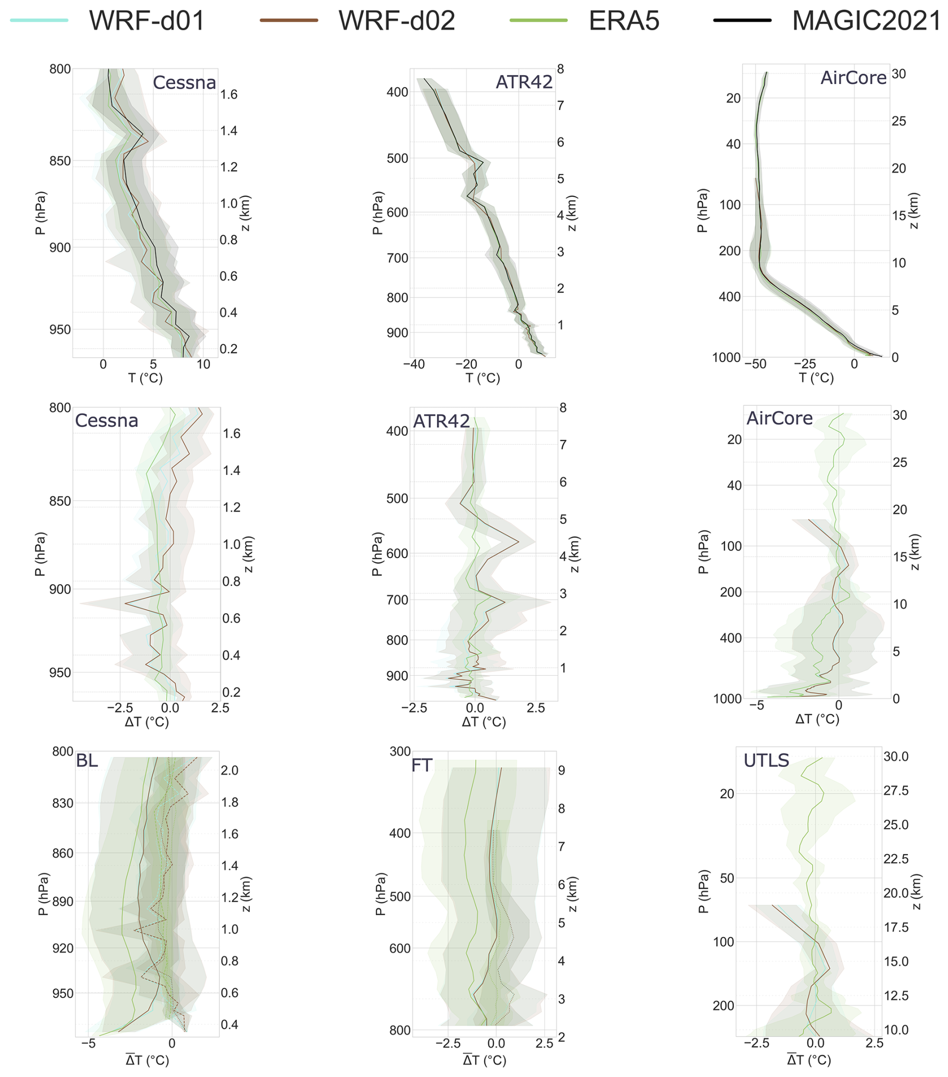
Figure A1 Temperature intercomparison between MAGIC2021 data and weather models. Profiles are computed using full weather balloon dataset and profile sections of ATR42 and Cessna flights. ERA5 related profiles are shown in green, WRF d01 in blue and WRF d02 in red. Top: Mean temperature profiles accross all flights from each platform (black) plotted with modelled temperatures interpolated on platform trajectories: Cessna (left), ATR42 (centre) and weather balloon (right). Middle: Temperature bias profile between for each platform: Cessna (left), ATR42 (centre) and weather balloon (right). Bottom: Sections of temperature bias profiles correponding to the 3 analysis levels: BL (left), FT (centre) and LS (right), where Cessna data is shown in dashed lines, ATR42 data in dotted lines and AirCore data in solid lines. Shaded areas represent the 1σ deviation from the mean temperature or temperature bias profiles.

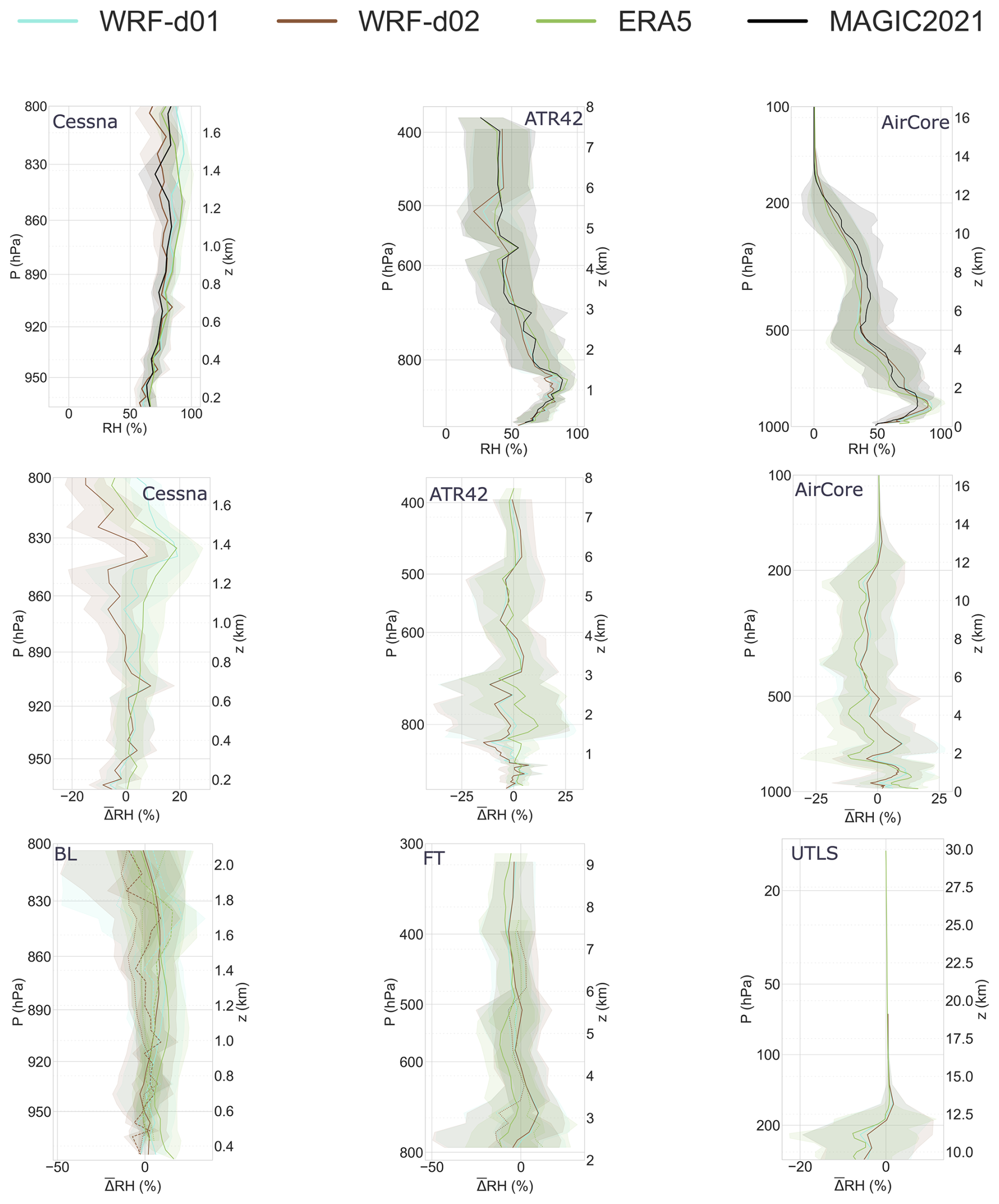
Figure A2 RH intercomparison between MAGIC2021 data and weather models. Profiles are computed using full weather balloon dataset and profile sections of ATR42 and Cessna flights. ERA5 related profiles are shown in green, WRF d01 in blue and WRF d02 in red. Top: Mean RH profiles accross all flights from each platform (black) plotted with modelled RH interpolated on platform trajectories: Cessna (left), ATR42 (centre) and weather balloon (right). Middle: RH bias profile for each platform: Cessna (left), ATR42 (centre) and weather balloon (right). Bottom: Sections of RH bias profiles correponding to the 3 analysis levels: BL (left), FT (centre) and LS (right), where Cessna data is shown in dashed lines, ATR42 data in dotted lines and AirCore data in solid lines. Shaded areas represent the 1σ deviation from the mean RH or RH bias profiles.

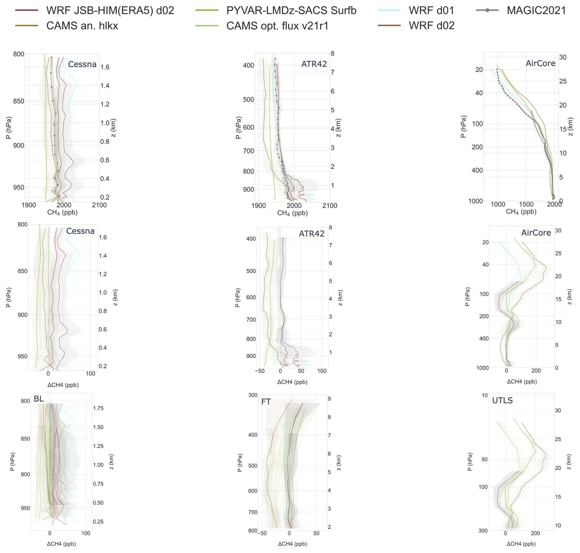
Figure A3 Methane intercomparison between MAGIC2021 data and chemistry-transport models. Profiles are computed using the full AirCore dataset and profile sections of ATR42 and Cessna flights. Top: Mean CH₄ profiles accross all flights from each platform (dotted grey line) plotted with modelled CH₄ interpolated on platform trajectories: Cessna (left), ATR42 (centre) and weather balloon (right). Middle:CH₄ bas profile for each platform: Cessna (left), ATR42 (centre) and weather balloon (right). Bottom: Sections of CH₄ bias profiles correponding to the 3 analysis levels: BL (left), FT (centre) and LS (right), where Cessna data is shown in dashed lines, ATR42 data in dotted lines and AirCore data in solid lines. Shaded areas represent the 1σ deviation from the mean CH₄ or CH₄ bias profiles.

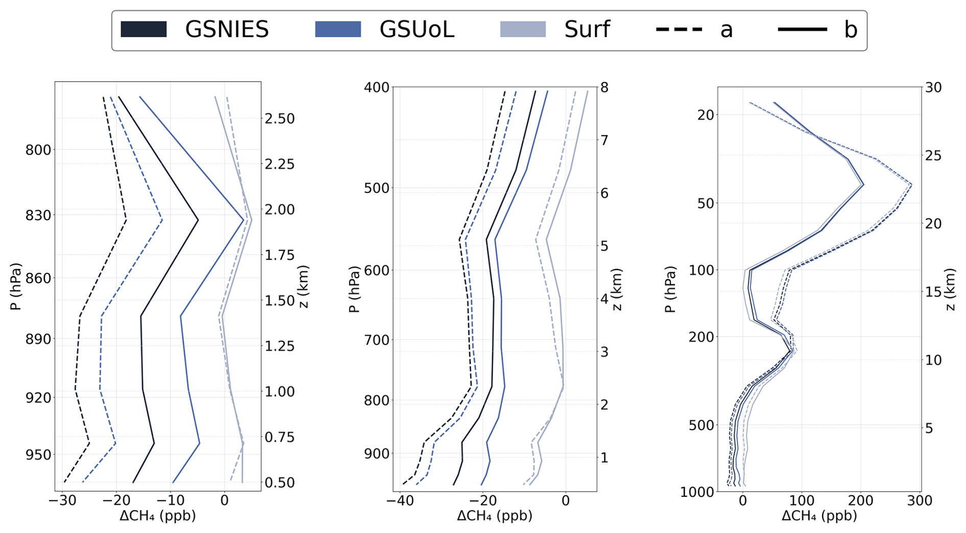
Figure A4 Mean PYVAR-LMDz-SACS bias from all 6 configurations computed with MAGIC2021 data: Cessna (left), ATR42 (middle) and AirCore (right) measurements.