Measurement of soluble aerosol trace elements: inter-laboratory comparison of eight leaching protocols

A range of leaching protocols have been used to measure the soluble fraction of aerosol trace elements worldwide, and therefore these measurements may not be directly comparable. This work presents the first large-scale international laboratory intercomparison study for aerosol trace element leaching protocols. Eight widely-used protocols are compared using 33 samples that were subdivided and distributed to all participants. Protocols used ultrapure water, ammonium acetate, or acetic acid (the so-called “Berger leach”) as leaching solutions, although none of the protocols were identical to any other. The ultrapure water leach resulted in significantly lower soluble fractions, when compared to the ammonium acetate leach or the Berger leach. For Al, Cu, Fe and Mn, the ammonium acetate leach resulted in significantly lower soluble fractions than those obtained with the Berger leach, suggesting that categorizing these two methods together as “strong leach” in global databases is potentially misleading. Among the ultrapure water leaching methods, major differences seemed related to specific protocol features rather than the use of a batch or a flow-through technique. Differences in trace element solubilization among leach solutions were apparent for aerosols with different sources or transport histories, and further studies of this type are recommended on aerosols from other regions. We encourage the development of “best practices” guidance on analytical protocols, data treatment and data validation in order to reduce the variability in soluble aerosol trace element data reported. These developments will improve understanding of the impact of atmospheric deposition on ocean ecosystems and climate.

1 Introduction

Atmospheric deposition has been a major pathway for vital nutrients, including trace elements, to reach the surface ocean over modern and geological times (Jickells et al., 2005; Jaccard et al., 2013; Mahowald et al., 2018). Natural ocean fertilization events have been reported following aeolian deposition of the vital micronutrient iron (Fe) from dust (Cassar et al., 2007), volcanic emissions (Langmann et al., 2010) and fire emissions (Tang et al., 2021). Since the Industrial Revolution, increasing atmospheric emissions linked to human activities as well as changes in anthropogenic land use have resulted in additional inputs of trace elements into the atmosphere (Mahowald et al., 2018; Bai et al., 2023). Notably, the increased emission of toxic metals (e.g., Cu) has been shown to have the potential to negatively impact marine ecosystems (Paytan et al., 2009; Jordi et al., 2012).

While anthropogenic activities may result in the emission of trace elements which are deleterious to the marine ecosystem, anthropogenic emissions are also rich in bioavailable essential nutrients, such as Fe (Hamilton et al., 2020; Ito et al., 2021) and Mn (Lu et al., 2024). In addition, atmospheric mixing with anthropogenic pollutants can enhance the solubility of natural aerosol Fe (and perhaps other trace elements) due to proton-promoted and ligand-mediated interactions (Shi et al., 2012; Paris and Desboeufs, 2013; Baker et al., 2021).

The biogeochemical impacts of aerosol trace elements deposited to the ocean are primarily driven by the fraction that is assimilated by the marine microbial community (Baker and Croot, 2010; Jickells et al., 2016; Mahowald et al., 2018). This fraction has historically been related to operational definitions of trace elements released into solution in experimental studies that have employed a wide variety of leaching protocols (e.g., Sholkovitz et al., 2012; Fishwick et al., 2014; Perron et al., 2020a; Li et al., 2023) and have variously described the released trace element fraction as “soluble”, “labile”, “leachable”, “dissolved”, “readily-accessible”, “bioaccessible” and “bioavailable”. Thus, while a considerable number of studies have investigated aerosol soluble trace elements (e.g., Hsu et al., 2005; Baker and Jickells, 2006; Buck et al., 2010; Kumar et al., 2010; Sholkovitz et al., 2012; Gao et al., 2020; Perron et al., 2020b; Chen et al., 2024), data reported in the literature suffers from a lack of standardization of protocols and terminology (Meskhidze et al., 2019). In addition, such operationally defined fractions do not map onto the oceanic definitions of “soluble” or “dissolved” trace elements in seawater, and understanding of the relationships between these fractions and the metabolic processes of nutrient uptake by marine organisms is currently lacking.

Further complication arises due to the solubilization of aerosol trace elements after deposition into the ocean, which can be influenced by varying properties of seawater, as well as through dissolution kinetics during the lifetime of particles in the seawater column that are difficult to replicate in the laboratory (Baker and Croot, 2010). Different leaching protocols may therefore simulate the solubilization of aerosol trace elements under different atmospheric and oceanic conditions as well as over different timescales, but the environmental relevance of the various leaching protocols in use is currently unclear.

The GEOTRACES community has made significant advances in producing a series of recommendations for aerosol sampling, sample handling and sample digestion for total trace element determination (Morton et al., 2013; Aguilar-Islas et al., 2024; Buck et al., 2024). Similar standardization has not been applied to aerosol soluble trace element determination, rendering both comparisons between different studies and data conglomeration for use in modeling studies very difficult (Perron et al., 2024; Shelley et al., 2024).

Several studies (Chen et al., 2006; Mackey et al., 2015; Clough et al., 2019; Perron et al., 2020a; Li et al., 2023) have compared aerosol trace element leaching methods and assessed the effects of different leaching solutions and contact time, although in each of these studies laboratory handling was performed by a single group and analysis was undertaken typically using a single instrument. A recent study (Li et al., 2024) found good agreement between aerosol solubility for eight trace elements measured by two laboratories using four different ultrapure water (UPW) batch leaching methods. Moreover, Li et al. (2024) suggested that very small and sometimes non-significant differences are introduced by varying agitation method, filter pore size and contact time within UPW batch leaching protocols.

Here we present the first large-scale intercomparison study that compares eight commonly used leaching protocols for determining soluble trace elements in aerosol samples. Six research institutions participated in this intercomparison: Guangzhou Institute of Geochemistry (GIG), China; the CSIR-National Institute of Oceanography (NIO), India; the University of East Anglia (UEA), UK; the University of Georgia (UGA), USA; the University of Plymouth (UoP), UK; and the University of Tasmania (UTAS), Australia. Leaching protocols examined use UPW, ammonium acetate (AmmAc) or acetic acid with hydroxylamine hydrochloride (Berger) as leaching solutions. These protocols also varied in contact time, agitation method and filtration procedure. No attempt was made to standardize the sample processing, analysis and the data treatment, with each group using their usual practices for these procedures. The aim of this study is to assess the extent to which the variability in the reported soluble fractions of aerosol trace elements can be attributed to the leaching methodology used and/or sample characteristics.

2 Methodology

2.1 Sample collection

This work used a custom-made instrument (ASM-1) (Jiang et al., 2022; Li et al., 2024) to collect ambient PM₁₀ (particulate matters with aerodynamic diameters of 10 µm or less) samples with a sampling flow rate of 1 m³ min⁻¹. Whatman 41 cellulose fiber filters (203 mm × 254 mm) were used to collect aerosol particles due to their low background (blank concentrations) for trace elements following the recommended GEOTRACES cleaning protocol. The actual area available for aerosol collection was 180 mm × 230 mm due to filter edges being covered by the frame of the filter holder. Filters used for aerosol sampling were acid-washed using procedures described in previous work (Morton et al., 2013; Zhang et al., 2022) to further reduce the background, and stored individually in zipper-top polyethene bags (Sigma-Aldrich, 229 mm × 305 mm).

Six PM₁₀ samples were collected at an urban site (113°36^′ E, 23°13^′ N) in Guangzhou from 24 November to 1 December 2021 to test aerosol trace element distribution on the filters (Table 1). The sampling site is located on the rooftop of a building at the Guangzhou Institute of Geochemistry, about 30 m a.g.l. (Yu et al., 2020). Sampling started at 08:30 or 20:30 each day (UTC+8), and lasted for 11.5, 23.5 or 35.5 h to intentionally vary the amount of aerosol particles collected over a large range. In addition, three lab blanks (i.e., acid-washed filters which were not taken to the field) and four field blanks (i.e., acid-washed filters mounted in the aerosol sampler for 2 h while the pump was off) were prepared during this sampling period.

Table 1 Summary of the aerosol samples collected in this study, their distribution among the participants and the purposes for which they were used.

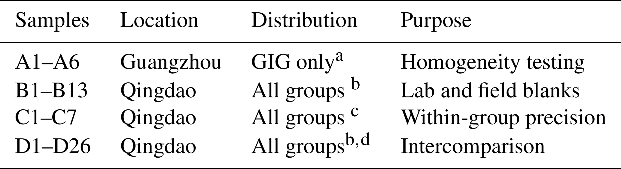
^a all eight subsamples of every sample, ^b one subsample of every sample; ^c three subsamples of two samples; ^d filtered air volume was 59 m³ for each subsample)

Another 33 PM₁₀ samples were collected between 3 April and 7 May 2022 at a suburban site in Qingdao (Table 1), a coastal city in Northern China affected by Asian desert dust and anthropogenic pollution. The sampling site is located on the rooftop of a building (36.34° N, 120.67° E), about 20 m a.g.l. (Zhang et al., 2022). Aerosol sampling started at 08:00 each day and ended at 07:30 on the next day (UTC+8), giving a sampling time of 23.5 h and a sampled air volume of 1410 m³. In addition, six lab blanks and seven field blanks were collected during the sampling period in Qingdao with the same procedure as described above.

After sampling, each filter was folded inward to protect aerosol particles, placed back into the zipper-top polyethene bag, and stored frozen at −20 °C.

2.2 Sample use and distribution

All the PM₁₀ samples and blank filters were divided into eight discs (47 mm in diameter) using a circular titanium hole-punch. These subsamples were folded inward, stored individually in zipper bags (Sigma-Aldrich, 64 mm × 76 mm), and labelled X-1 to X-8 (where X is the sample identification name). Subsamples were labelled after subdivision, hence the subsample numbers are not related to the location of the discs on the filter.

Intercomparison exercises should ideally be conducted by sharing homogeneous materials among the participants in quantities that are sufficient for each participant to make a realistic assessment of the precision of their measurements. Neither of these conditions could be easily met for the intercomparison study reported here because: (1) it could not be guaranteed that aerosol material was homogeneously distributed over the aerosol filters; and (2) the amount of material a subsample contained was unlikely to be sufficient for replicate analysis of the soluble trace elements studied. Our study therefore addressed the issues of sample homogeneity (Sect. 2.6.1), intra-method precision (Sect. 2.6.2) and inter-method comparison (Sect. 2.6.3) separately.

For the homogeneity test, all eight portions of each filter collected at Guangzhou (A1-A6) were subjected to the same digestion procedure by a single group at GIG (Sect. 2.3) to determine the total concentration of 14 trace elements in each subsample. This information directly informs whether sample heterogeneity represents a confounding factor in later comparisons.

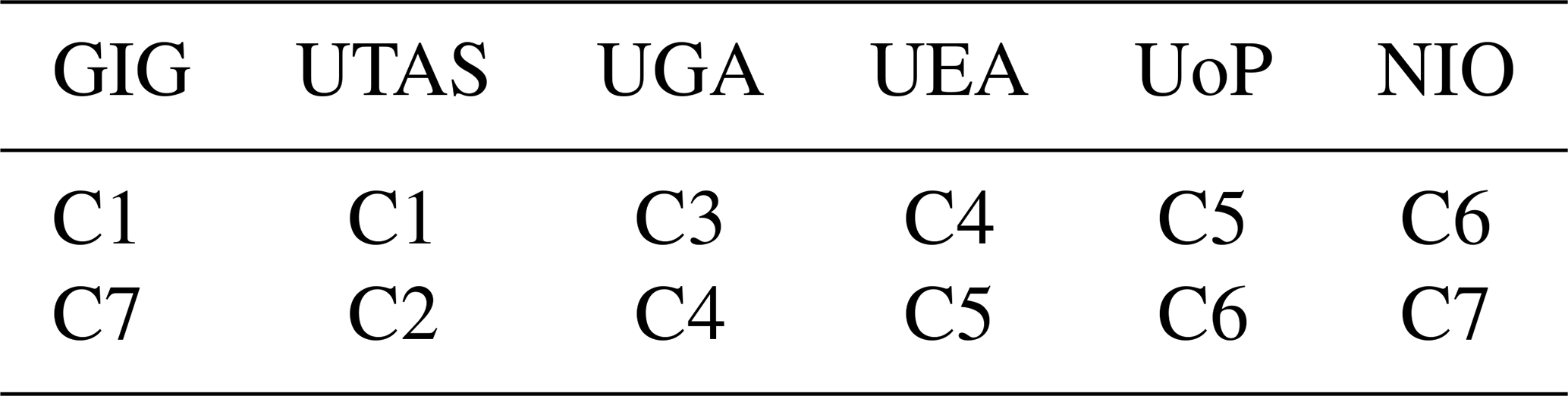
The 33 samples (and six lab blanks and seven field blanks, B1–B13) collected in Qingdao were distributed to all participating laboratories for soluble trace element analysis. Seven of these samples (C1–C7) were used to assess intra-method precision with each laboratory receiving three subsamples of two filter samples (Table 2). Furthermore, each laboratory received one portion of each of the remaining 26 filter samples (D1–D26) for conducting the leaching method intercomparison. These sub-samples (D1–D26) each had a sampled air volume of 59 m³, which can be used to convert data presented in this study into atmospheric concentrations. One subsample of each of the Qingdao samples was also retained at GIG for total trace element determination, and the last subsample was reserved for future as yet undetermined usage.

Table 2 Summary of subsample distribution from filter samples in group C to the six laboratories. Each lab was provided with triplicate subsamples of each C filter.

2.3 Leaching and digestion procedures

Table 3 provides an overview of the laboratory leaching protocols investigated in this study; more details can be found in Tables S1–S6 in the Supplement. Each laboratory analyzed the samples they received using only the method associated with them in Table 3. UGA and UTAS both employed a two-stage protocol with successive leaching (termed leach 1 and leach 2, hereafter) and therefore reported two values for each trace element. A total of eight leaching protocols were examined in this study.

Table 3 Overview of the eight leaching protocols used by the six laboratories participating in this intercomparison study.

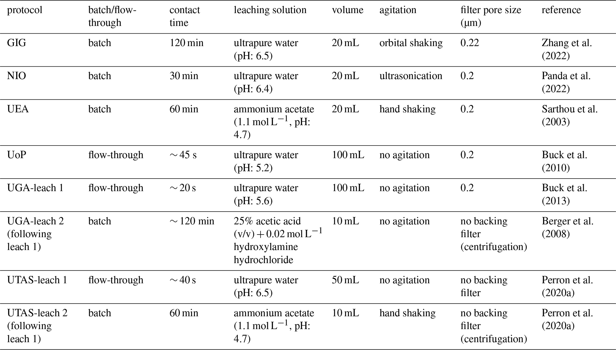
The eight leaching protocols fell into three broad categories based on the chemistry of the leaching solution: five methods used ultrapure water (> 18.2 MΩ cm) as leachate (two employing batch extraction and three employing flow-through extraction), while the other three methods used ammonium acetate (two methods) or acetic acid and hydroxylamine hydrochloride (one method) as leachate. These categories are referred to hereafter as UPW, AmmAc and Berger leaches, respectively. Within and among these categories, protocols also differed in solution contact time, volume of leachate, presence or absence of agitation, additional filtration step using a backing filter, and pore size of any backing filter, as summarized in Table 3. Thus, it is important to note that, even within each of the three categories of methods, no leaching protocol examined in this study was identical to any other.

Results are presented hereafter using the acronym of the laboratory followed by the type of leaching solution used (“-u” for UPW, “-a” for AmmAc and “-b” for Berger). Where groups performed sequential leaching (Table 3), we consider the sum of both leaching fractions to be equivalent to a single-step AmmAc (for UTAS-a) or Berger (for UGA-b) leach. In this work, we report results produced using eight different leaching protocols (i.e. GIG-u, NIO-u, UEA-a, UTAS-u, UTAS-a, UGA-u, UGA-b, and UoP-u).

The digestion procedure used by the GIG laboratory to measure total trace elements contained in aerosols was described previously (Zhang et al., 2022). Briefly, aerosol filter subsamples were digested in a mixture of HNO₃, H₂O₂ and HF in an acid-cleaned Teflon jar, using microwave digestion. The residual solution was then evaporated, and 20 mL HNO₃ (1 %) was added to the jar. The resulting solution was filtered through a 0.22 µm polyethersulfone filter and analyzed using inductively coupled plasma mass spectrometry (ICP-MS, iCAP Q, Thermo Fisher Scientific).

2.4 Trace element determination

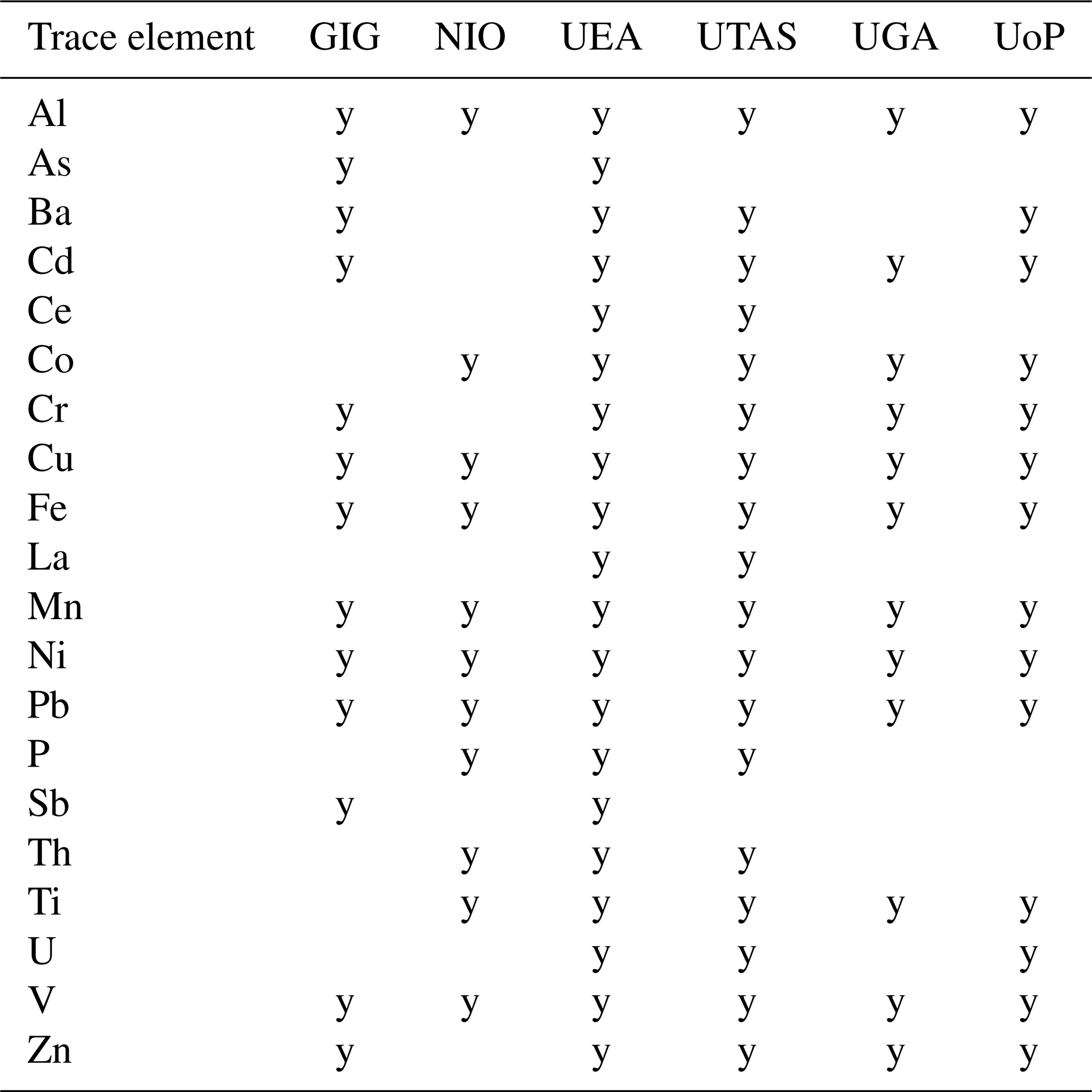
Each group determined trace elements in the leaching solutions using the analytical methods routinely used in their laboratory. Table 4 shows the trace elements determined by each laboratory, Table S7 summarizes the methods used, and Table S8 provides a summary of the analytical detection limits. As shown in Table 4, up to 20 trace elements were determined by groups participating in this intercomparison study. The results presented in this paper focus on the seven trace elements (i.e., Al, Cu, Fe, Mn, Ni, Pb and V) that were determined by all the six groups. Comparisons for the other elements (Ba, Cd, Ce, Co, Cr, La, P, Th, Ti, U and Zn) are reported in the Supplement (Figs. S1 and S3–S6). For all groups, the mass of trace elements in aerosol samples was determined against an external standard calibration (Table S7). The same trace elements determined in leaching solutions by GIG were also determined in the total digests of the Guangzhou and Qingdao samples. Trace elements concentrations in leachate and digests were corrected for the volume of the liquid phase used and reported as mass of trace elements on the filter subsamples received.

Table 4 List of trace elements determined by each of the six laboratories. If one trace element was not measured by one laboratory, the corresponding cell is left blank.

2.5 Blank subtraction

For each analytical method, blank subtraction was conducted using the following procedure.

As described above, each group received 13 blank filters (B1–B13). First, we calculated the median of all the blank measurements generated by a research group. If the median value was below the analytical detection limit for that trace element and analytical method, no blank correction was made; if the median was above the analytical detection limit, this median value was subtracted from the respective measured quantity for the subsample. We calculated the median absolute deviation (MAD, defined as the median of the absolute differences between the individual blanks and the median blank) to represent the uncertainty in the blank. Subsamples with blank-corrected quantities less than three times of the MAD were defined as less than the blank-correction detection limit. In this work we use median and MAD, rather than mean and standard deviation, because median and MAD can be reliably calculated when values below detection limits are present and they are less affected by the presence of outliers.

2.6 Data analysis

2.6.1 Sample homogeneity

Six samples (A1–A6) were collected in Guangzhou to examine particle distribution homogeneity, and eight subsamples (47 mm discs) were obtained from each sample. For each filter sample, we measured the mass of 14 trace elements in the eight subsamples (X_i, where X_i is the mass of a given trace element in the ith subsample) at the GIG laboratory; we then calculated the median value (X_m) of the eight measurements, the MAD as well as relative MAD, which is defined as MAD/X_m.

2.6.2 Precision derived from replicate subsample analysis

Each group measured trace elements on three subsamples from each of two different aerosol samples (C samples) collected at Qingdao (Table 2). For each trace element, the relative MAD was determined for both samples and the higher of these values was used as the uncertainty in the soluble trace element mass measurement. This value was then applied to the intercomparison study samples (D1–D26) for which no replicate sample was available. We note that the uncertainty determined in this way includes a component due to the heterogeneity of trace element distribution across the aerosol samples, as well as a component from variability in the analytical procedures within each group.

For four (GIG, NIO, UGA and UTAS) of the six groups participating this work, the magnitude of the uncertainty in each intercomparison subsample was determined by multiplying its measured soluble mass by its respective relative MAD value. The other two groups (UEA and UoP) reported individual uncertainties for the intercomparison subsamples based on calibration uncertainties and repeated analyses of single subsample extract solutions. In the latter cases, the uncertainties of the soluble trace element mass measurement in individual subsamples were taken to be whichever of the replicate-determined or individually-determined uncertainties was larger.

2.6.3 Inter-method statistical comparisons

Comparison of the results produced by the various leaching methods for each trace element for samples D1–D26 was done where possible using both parametric and non-parametric tests, and each dataset for each element and method was tested for normality using the Shapiro Wilks method (Miller and Miller, 2010). For comparisons of similar methods (e.g., the batch UPW leaches of GIG and NIO) the hypothesis that each method-method pair produced statistically indistinguishable results was examined according to the following statistical tests.

1. Spearman's Rank Correlation was used to test the correlation between methods (assuming that there is a direct relationship between the amounts of a trace element leached by the two methods). When no correlation was found between two methods, subsequent tests were deemed to be unreliable.

2. A two-tailed t-test was used to test the slope of a method-method relationship. Method-method slopes and intercepts were determined using orthogonal distance regression (ODR), since both analytical parameters were subject to significant uncertainty and simple linear regression was therefore not suitable. A slope equal to 1 implies that sample-to-sample changes in trace element release are equivalent between the two methods. Because the samples shared for the intercomparison were subject to heterogeneity, the slope was also tested for difference to 1 ± 0.12, after uncertainties due to sample heterogeneity were taken into account (the upper limit of such uncertainties is estimated to be 12 %, as discussed in Sects. 2.6.1 and 3.1); in this case, one-tailed t-tests were used.

3. A two-tailed t-test was used to investigate whether the intercept of the ODR method-method relationship differed significantly from zero. Divergence from zero indicates the presence of an offset between the two methods.

4. Paired t-tests and Wilcoxon Signed Rank tests were used to assess if the difference between the two measurements for each individual sample was different from zero.

Optimum agreement between each method-method pair was therefore indicated by significant correlation (test 1) and absence of significant differences indicated by tests 2–4.

Comparisons between dissimilar methods (e.g. batch UPW vs AmmAc) were made using two-tailed t-tests and Mann Whitney U tests, after first confirming the presence of significant differences between the datasets using one-way ANOVA and Kruskal Wallis tests.

2.7 Air mass back trajectory analysis

Five-day air mass back trajectories (AMBTs) were calculated at heights of 50, 500 and 1000 m a.g.l. throughout the sampling period at the sampling site in Qingdao, using the NOAA READY HYSPLIT model with NCEP/NCAR Reanalysis Project datasets (Stein et al., 2015). For each sample, trajectories were calculated every 3 h throughout the collection period and 50 m trajectories (for all samples) were used to perform cluster analysis with the openair software tool in R (Carslaw and Ropkins, 2012). Between four and six clusters were tested for this analysis, and three clusters (arrivals from the north (N), southwest (SW) and the Yellow Sea (YS)) were chosen to represent the major differences in atmospheric transport pathways during the field sampling (Fig. 1). Each sample was assigned to one of the three clusters, based on the dominant AMBT type of the eight trajectories calculated for that sample.

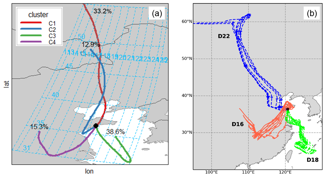
Figure 1 (a) Result of the 4-cluster analysis of the AMBTs calculated during the sample collection at Qingdao, showing representative pathways for the clusters and their percentage occurrence; (b) examples of 50 m AMBTs for samples classified as N (Sample D22, blue dash), SW (D16, red solid) and YS (D18, green dot-dash) types.

3 Results and Discussion

3.1 Aerosol trace element distribution on the filters

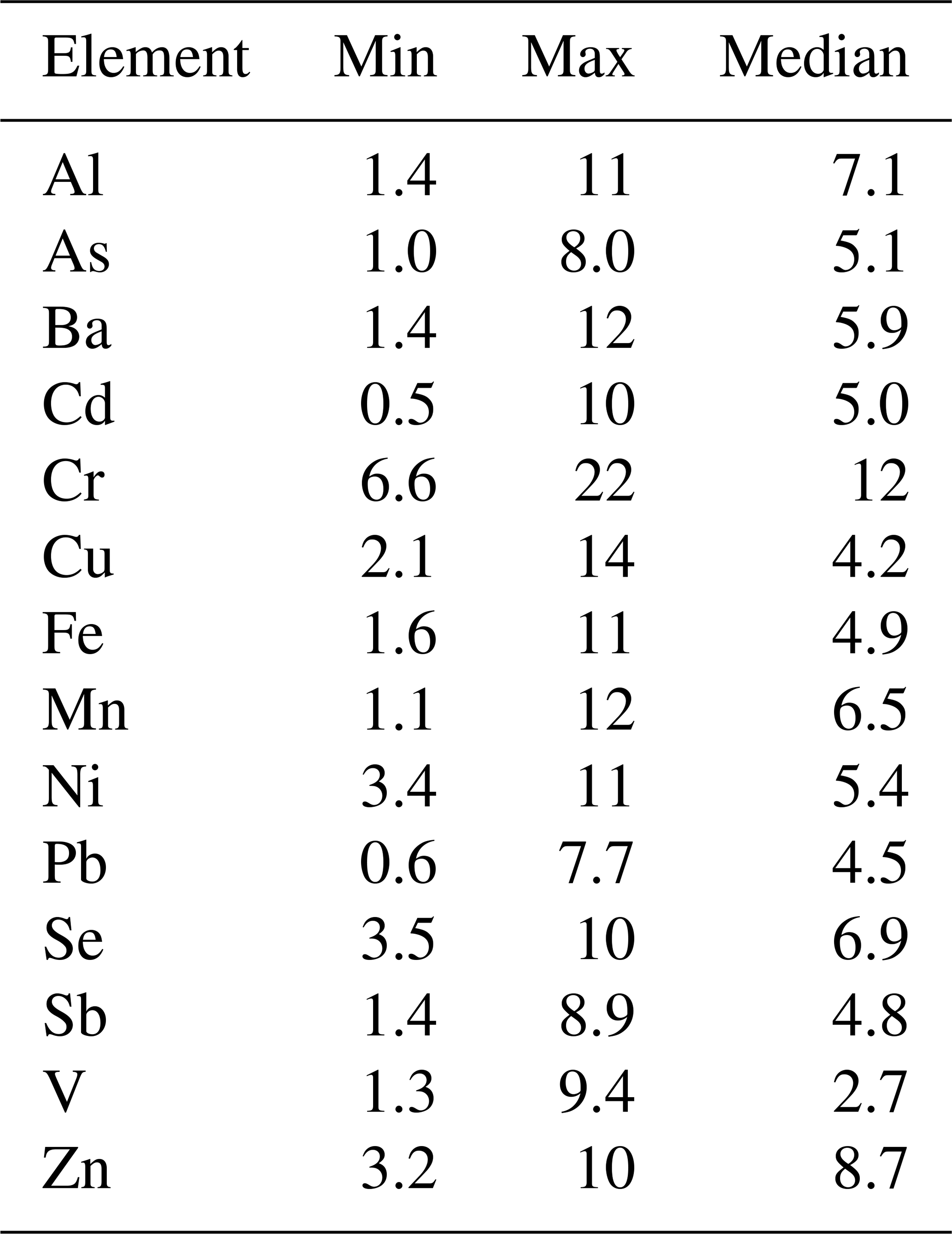
Table 5 summarizes the relative MAD values obtained for total trace elements contained in the Guangzhou samples (A1–A6). The median of relative MAD values obtained for the 14 trace elements ranged from a minimum of 2.7 % for V to a maximum of 12 % for Cr. In this work, we chose a conservative approach by applying the highest median relative MAD value (i.e. 12 %) to represent the uncertainty associated with trace element distribution heterogeneity over a filter, regardless of the element analyzed. Variations between different methods greater than this 12 % heterogeneity are likely to be due to differences in analytical results, as described in Sect. 2.6.3.

Table 5 Summary of the relative MAD (in %) in particle distribution homogeneity: minimum, maximum and median values for the 6 filters collected in Guangzhou.

3.2 Background (blank) contribution

Each research group determined the soluble fraction of trace elements in blank samples (B samples) according to their chosen method(s); therefore, the blank values included the contribution from the blank filters and from the analytical procedures used. The total blank for each trace element analyzed was subtracted from the subsamples' measurements in the intercomparison study, without attempting to separately quantify the contributions from the filter and the analytical procedure.

In almost all cases, blank contributions were extremely low with respect to the PM₁₀ subsamples. For the seven elements that are the focus of this intercomparison study, 79 % of blanks were below the analytical detection limit, and only two blank values were greater than 10 % of the magnitude of the lowest intercomparison sample. There were only a few cases for which blanks were higher than the lowest intercomparison sample and 24 cases (∼ 2 %) where intercomparison samples were identified as being below the blank-correction detection limit. Table S9 summarizes the blank contributions for all trace elements with measurable blanks.

3.3 Intra-method precision

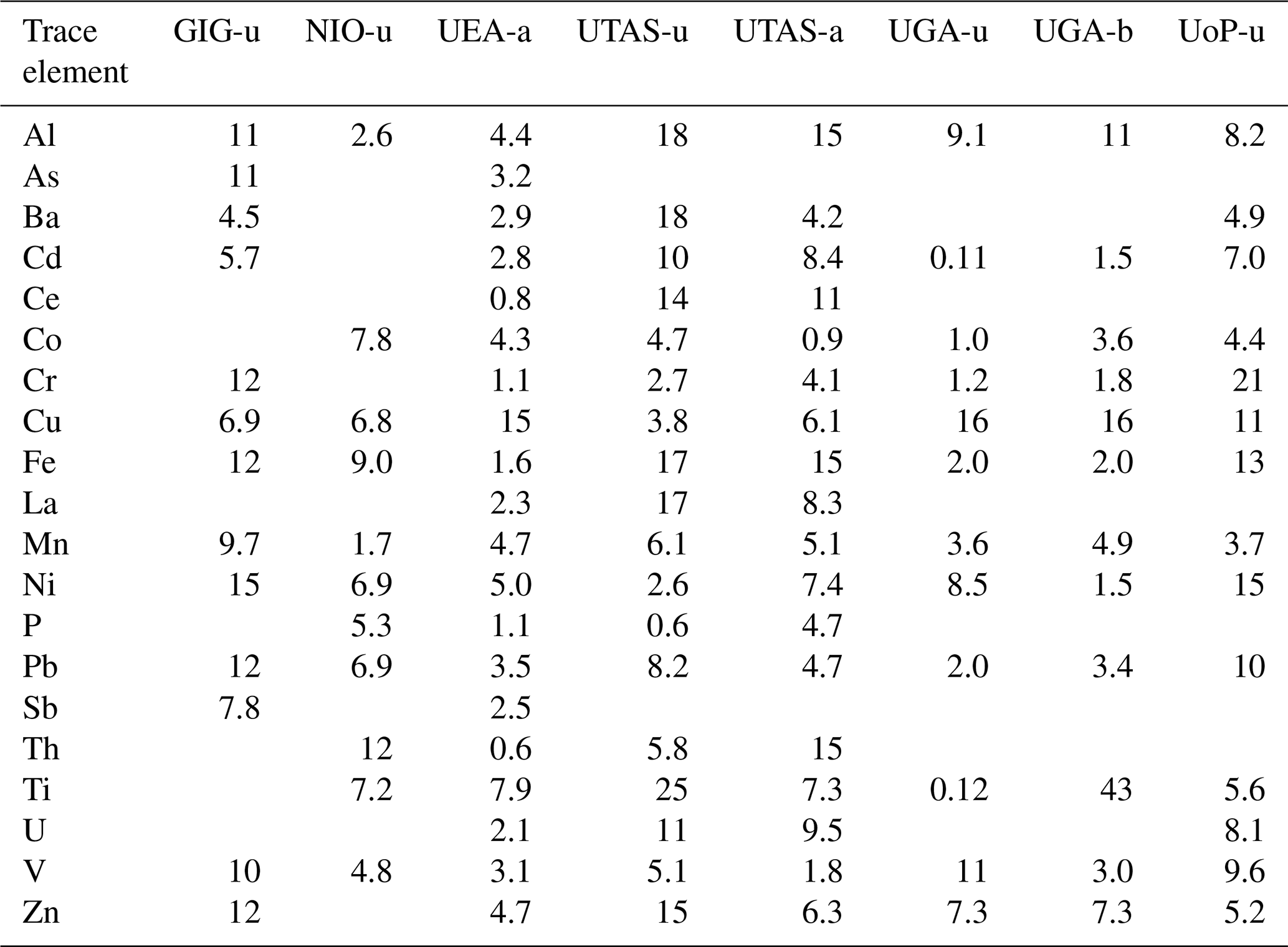
Table 6 summarizes the relative uncertainties (in %) for soluble trace elements determined by each of the six groups when analyzing three replicates of the same aerosol sample (C samples), and the relative uncertainty is defined in Sect. 2.6.2. In most cases these relative uncertainties were within the range of values determined for total element homogeneity over whole filter samples (Table 5). None of the uncertainties reported in Table 6 was larger than the highest uncertainty value reported for the total element homogeneity test (22 % for Cr), suggesting that intra-laboratory variability was not significantly greater than the variability between subsamples within individual filter samples.

Table 6 Summary of the relative uncertainties (in %) for soluble trace elements analysis of 3 replicate samples determined by each of the six laboratories. If one trace element was not measured by one laboratory, the corresponding cell is left blank.

3.4 Comparison of leaching methods

Figure 2 summarizes statistical comparisons of similar leaching methods for all of the samples collected at Qingdao (D samples), and the results are discussed below.

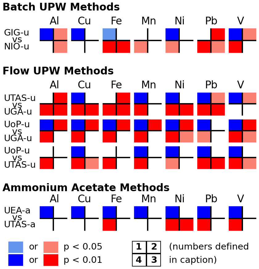
Figure 2 Summary of the statistical comparisons of the leaching methods for all of the 26 samples (N, SW and YS) collected at Qingdao. Comparisons are only shown for similar methods: Batch UPW (GIG-u and NIO-u), Flow UPW (UoP-u, UTAG-u and UGA-u) and AmmAc (UEA-a and UTAS-a). Statistical tests (as detailed in Sect. 2.6.3) shown in quadrants are (1) Spearman's Rank Correlation, (2) one-tailed t-test of slope versus 1 ± 0.12 uncertainty, (3) intercept equals zero, and (4) Wilcoxon Signed Rank Test. Significant test results are indicated by the color code: blue indicates agreement between methods, red indicates disagreement, and white indicates that the test result was not statistically significant. Full statistical test results (all tests and elements) can be found in Fig. S4.

3.4.1 Ultrapure water batch leaching methods

Table 3 shows that the two UPW batch leaching protocols examined in this work differ in contact time (2 versus 0.5 h), agitation method (orbital shaking versus ultrasonication), and to a lesser extent, filter pore size (0.22 versus 0.2 µm).

As shown in Fig. 2, a strong correlation (Spearman test, p<0.01) was observed between soluble trace element masses measured by GIG and NIO for four of the elements investigated (Al, Cu, Ni and V); nevertheless, the slope statistically differs from 1 ± 0.12 for Al and V and the intercept is statistically different from zero in the case of Al (p<0.05). Among these four elements, the best agreement between the two protocols was found for Cu and Ni (Fig. 3), with NIO values slightly higher than those of GIG, except for a few YS samples. Good agreement was also observed for Al and V, although for both elements there are some samples with measured values greatly deviating from the 1:1 line.

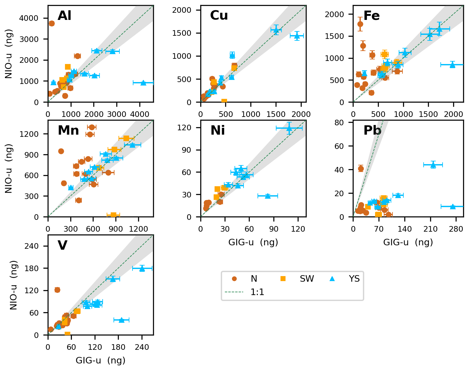
Figure 3 Comparison of the absolute mass of soluble trace elements (Al, Cu, Fe, Mn, Ni, Pb and V) obtained using UPW batch leaching methods (GIG and NIO). Air mass origins (N, SW, YS) for each sample are indicated by the color code. The dashed line indicates the 1:1 relationship between the methods, and the grey shading indicates the 12 % sample homogeneity uncertainty.

Although there was a significant correlation for Fe (Spearman test, p<0.05, Fig. 2), large deviation from the 1:1 slope was not uncommon (Fig. 3). Fe measured by NIO tended to be higher than GIG values, especially for samples from continental air masses (N and SW). No significant correlation was found between the two methods for Mn or Pb (Fig. 2). Similar to Fe, soluble Mn values reported by NIO tended to be higher than those reported by GIG (Fig. 3), especially for N and SW samples. The ultrasonication used by NIO may lead to the formation of reactive oxygen species (e.g., hydroxyl radicals and hydrogen peroxide) due to acoustic cavitation (Kanthale et al., 2008; Miljevic et al., 2014). These species have the potential to reduce insoluble Fe(III) and Mn(IV) to the more soluble Fe(II) and Mn(II), especially when poorly soluble mineral dust is present in the N and SW samples. Enhanced solubility of Al in the NIO data (relative to GIG) is not observed, perhaps because Al only has one oxidation state and its solubility may not be affected by redox chemistry.

Notably, NIO reported much lower values than GIG for Pb (Fig. 3). GIG and NIO both checked their experimental data and found no errors, and there is no clear clue why such large differences occurred. Therefore, here we do not discuss the UPW batch data for Pb further.

3.4.2 Ultrapure water flow-through leaching methods

The three UPW flow-through leaching methods investigated here differ by contact time, pH and volume of leaching solution, and the use (or not) of a backing filter (Table 3).

Overall, a positive and significant correlation (Spearman test p<0.01, Fig. 2) was found between the soluble trace element mass measured by UoP and UGA. For all trace elements except Pb, the comparison of these two methods, however, resulted in a slope different from 1 ± 0.12 and an intercept different from 0 for Ni and V (Fig. 2), with slightly lower values obtained by UoP than by UGA (Fig. 4). This difference cannot be attributed to higher blank levels in UGA samples because both laboratories had element blanks below their method detection limits (hence, no blank correction was applied).

The UTAS UPW flow-through method produced soluble trace element measurements that positively and significantly correlate with the two other methods (Fig. 2), except for Al and Fe. Overall, UTAS measurements were higher than those of UoP (Fig. 4), except for low Ni measurements (compared to both UoP and UGA) which result from elevated Ni blank correction in UTAS data treatment (due to new Ni cones used in the SF-ICP-MS instrument, Table S9).

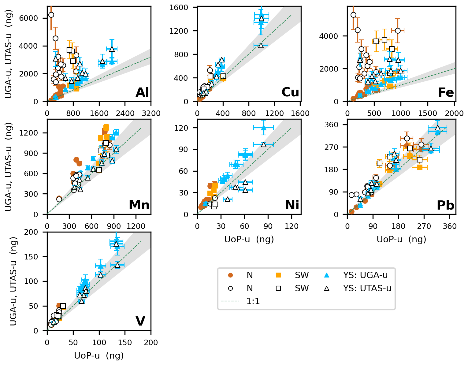
Figure 4 Comparison of the absolute mass of soluble trace elements (Al, Cu, Fe, Mn, Ni, Pb and V) obtained using UPW flow-through leaching methods (UoP, UTAS and UGA). Plot details are as described in Fig. 3. UGA data are represented by solid symbols, and UTAS data are represented by open symbols.

One striking observation from Figs. 2 and 4 is the lack of correlation between Al and Fe measured by UoP or UGA and that measured by UTAS (similar behavior was also observed for Ti, Ba and U, as shown in Fig. S1). High Al and Fe masses reported by UTAS could stem from the absence of a backing filter in the UTAS method, whereby the soluble fraction of trace elements measured can include the contribution of particles with a diameter greater than 0.2 µm. As shown in Figs. 4 and S2, this observation is even more obvious in aerosol samples influenced by terrestrial air-masses (N and SW samples) due to lower solubility of Fe and Al in these samples when compared to YS samples. The absence of a backing filter in the UTAS protocol only seems to influence lithogenic elements with lower solubility (Al, Fe, Ti, Ba, U), while more soluble elements (Cu, Mn, Ni, Pb and V) showed a significant correlation (p<0.01) with the other two methods investigated. No filtration in the UTAS UPW flow-through protocol may also be responsible for higher uncertainty obtained for lithogenic elements when measuring three replicate samples (Table 6).

Based on the intercomparison results, it is reasonable to assume that the different leaching solution volumes have minor, if any, impacts on the results from the three UPW flow-through leaching methods. Our findings are consistent with those of Winton et al. (2015) suggesting that over 90 % of the soluble Fe contained in aerosols was extracted using a single 50 mL UPW flow-through leach, although Winton et al. (2015) did not provide results for other trace elements.

3.4.3 Ammonium acetate leaching methods

As displayed in Table 3, the two AmmAc leaching protocols applied by UEA and UTAS differ by the volume of the leaching solution and the absence of a backing filter in the UTAS protocol; in addition, the UTAS leaching is performed as part of the sequential leaching of a single sample, immediately following the UPW flow-through leaching.

For Al, Cu and Mn, measurements show excellent agreement (significant correlation (p<0.01), and no significant differences in slopes, intercepts or soluble masses) for the two AmmAc methods (Figs. 2 and 5). The other elements (Fe, Ni, Pb and V) also show good agreement between methods, with no significant differences for slopes and only Ni having a significant difference for intercept, possibly due to the Ni blank overcorrection applied to the UTAS dataset (see Sect. 3.4.2 and Table S9) which shifts the correlation curve below the 1 ± 0.12 grey-shaded area in Fig. 5. Both Pb and V measurements show good correlation and agreement in intercept values, although the slopes differ from 1 ± 0.12 (Fig. 2). These four elements (Fe, Ni, Pb and V) do show significant differences for soluble masses, possibly due to differences in the calibration methods or other analytical differences.

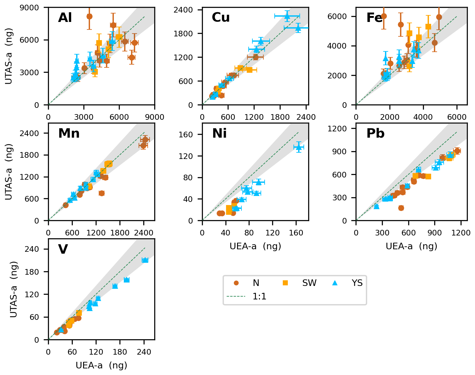
Figure 5 Comparison of the absolute mass of soluble trace elements (Al, Cu, Fe, Mn, Ni, Pb and V) obtained using AmmAc extraction methods (UEA and UTAS). Plot details are described in Fig. 3.

Poorer agreement between the two methods was again found for lithogenic elements (Al and Fe), although comparisons were noticeably better for the AmmAc methods (Fig. 5) than for the UTAS-u to other UPW flow-through method comparisons (Fig. 4). For these two elements (Al and Fe), measurement differences were more pronounced in samples influenced by “terrestrial” air masses (N and SW) while YS samples showed a good agreement (Figs. 5, S5 and S6). This better agreement for lithogenic elements between the AmmAc methods may suggest that the > 0.2 µm particles which are not removed by the UTAS UPW leaching protocol are largely soluble in AmmAc so that their trace element content is not removed by 0.2 µm filtration in the UEA method.

3.4.4 Influence of different leaching protocols on the determination of fractional solubility

Figure 6 illustrates the variations in solubility of trace elements in the Qingdao samples, determined using the eight leaching methods tested in this study. Kruskal Wallis and one-way ANOVA tests both indicated significant differences (p<0.01) among the results obtained for the five methods employing UPW as the leaching solution for all elements except Ni and V. Some of the significant differences within the UPW methods are discussed in Sect. 3.4.1–3.4.2 (e.g. for Pb in the UPW batch methods, and Al and Fe in the UPW flow-through methods). In general, where significant differences in solubility existed within the UPW group these did not appear to be related to whether the method employed batch or flow-through techniques.

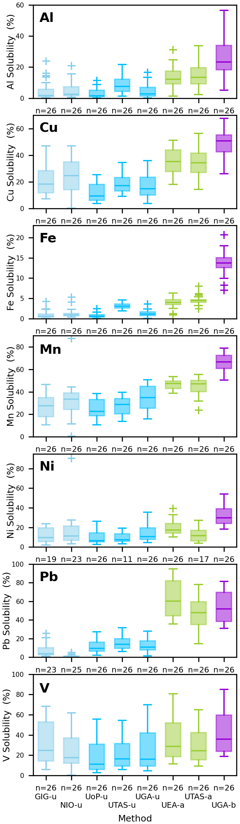
Figure 6 Box and whisker plots of solubility (in %) for Al, Cu, Fe, Mn, Ni, Pb and V in the Qingdao samples determined using the eight leaching protocols tested in this study. Colors indicate method type: batch UPW (light blue), flow UPW (dark blue), AmmAc (green), and acetic acid with hydroxylamine hydrochloride (purple).

When comparing all the eight methods, Kruskal Wallis and one-way ANOVA tests indicated significant differences in solubility for all seven elements. In almost all cases, the UPW methods resulted in significantly different (lower) solubilities than those obtained with the AmmAc and Berger leaches, as expected. For Al, Cu, Fe and Mn, solubilities obtained using the AmmAc leach were significantly different from (lower than) those obtained using the Berger leach.

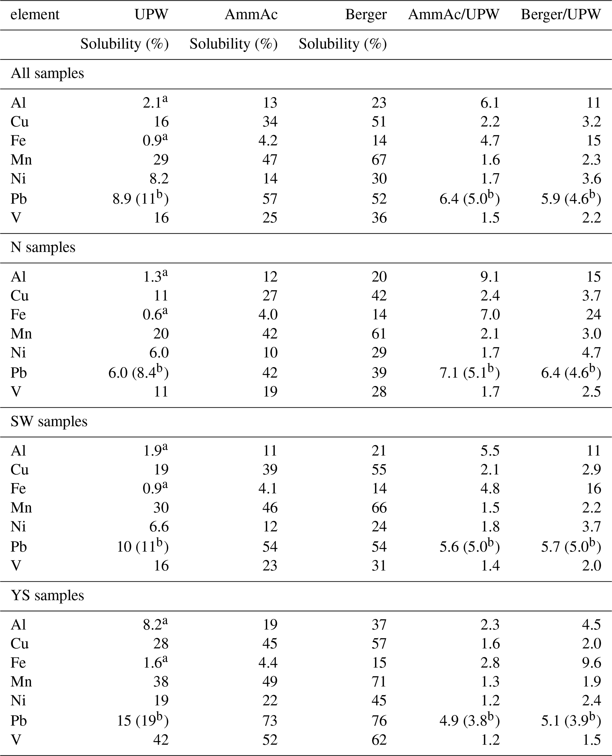
Table 7 illustrates the broad differences obtained between the UPW, AmmAc and Berger methods using the pooled median solubility values for each method. Both Fig. 6 and Table 7 show that the extent of solubilization from aerosol by the different methods is highly element specific. For example, the patterns in enhancement in solubility for AmmAc and Berger compared to UPW (AmmAc/UPW and Berger/UPW, see Table 7) are very different for Fe, Mn and Pb. Interestingly, the more aggressive conditions of the Berger leach (compared to AmmAc) had large impacts on the dissolution of poorly soluble lithogenic elements (such as Al and Fe), but no effect on Pb dissolution.

Table 7 Median trace element solubilities for the Qingdao aerosol samples, determined from the combined soluble element masses determined for the methods using UPW (GIG-u, NIO-u, UoP-u, UTAS-u and UGA-u), AmmAc (UEA-a and UTAS-a) and Berger (UGA-b), and solubility ratios of the AmmAc to UPW (AmmAc/UPW) and Berger to UPW (Berger/UPW) methods. (a: excluding UTAS-u due to the inclusion of > 0.2 µm particles, b: excluding GIG-u and NIO-u due to unexplained inconsistencies in Pb data).

For most methods, there were statistically significant differences (Kruskal Wallis and one-way ANOVA tests) between solubilities determined for the different air mass types for most elements (Figs. 7 and S7). Exceptions to this were the NIO-u results (for which significant differences were only found for Al and Cu) and Fe (for which significant differences were found for some of the UPW methods, but not for AmmAc or Berger). In all cases where such significant differences were found, solubility in YS-type samples was higher than that in N-type samples (Fig. 7). Note that the difference between N and YS samples appear to become less pronounced as the leach solution becomes more aggressive (e.g. for V, the YS/N solubility ratios are 4.0–6.1 for the UPW methods, 2.7–3.0 for the AmmAc methods, and 2.3 for the Berger method). Enhanced trace element solubility in YS samples compared to N samples may be due to increased atmospheric processing of particles transported over the ocean (particularly for lithogenic elements) (Longo et al., 2016; Hamilton et al., 2022; Sakata et al., 2023) or to anthropogenic emissions of highly soluble trace elements to the marine atmosphere (e.g. V, Ni from shipping) (Sholkovitz et al., 2009; Chen et al., 2024).

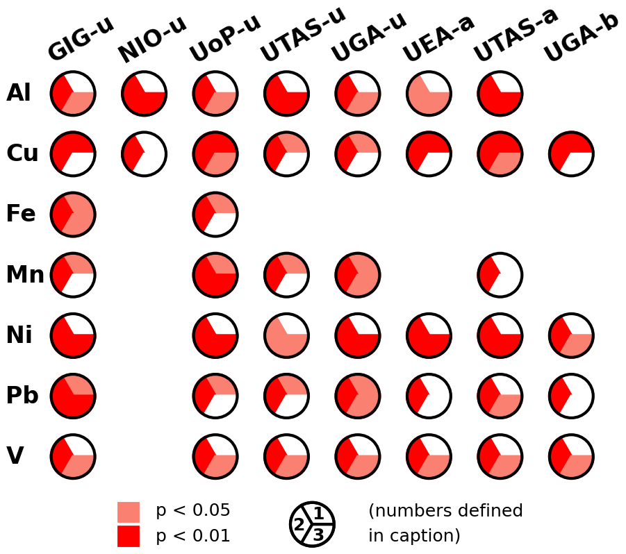
Figure 7 Summary of the comparisons of trace element solubility for the N, SW and YS samples determined using the eight leaching methods tested in this work. Red colors indicate statistically significant differences (Mann Whitney U Test) between pairs of sample types (1: N vs SW; 2: N vs YS; 3: SW vs YS), and white colors indicate no significant difference. No summary is shown where the Kruskal Wallis Test indicated no significant differences (p<0.01) between the three sample types.

The aerosol provenance seems to be a key driver of the resulting amount of total and soluble trace element measured, regardless of the leaching protocol used. Indeed, higher Al, Cu, Ni, and V solubility was determined for YS samples compared to samples showing terrestrial fingerprints. Such an increase in trace element solubility in marine samples was less pronounced when measuring Fe, Mn and Pb due to similarly high solubility measured in samples influenced by SW air-masses. In YS samples, V, Ni and Cu showed higher solubility in UPW, with a lesser impact of stronger AmmAc and Berger leaching protocols. Increased atmospheric processing of particles transported over the ocean can explain the presence of more readily soluble trace elements in the presence of UPW in YS samples compared to N and SW samples.

As opposed to the UPW leaches, AmmAc methods showed similar (Mn, Pb) or higher (Al, Fe) solubilities in samples containing terrestrial inputs, except for Cu, Ni and V for which higher solubility was found in samples influenced by marine air masses.

4 Conclusions and recommendations for future studies

In general, comparisons between similar leaching methods (Sect. 3.4.1–3.4.3) show a high degree of correlation between measured soluble masses of trace elements. Where correlation was poor, the differences appear to stem from specific differences in the leaching methods. For example, the use of ultrasonic agitation instead of mechanical agitation for UPW batch methods seems to result in increased solubility for Fe and Mn, and the absence of a backing-filter resulted in higher soluble Al and Fe in the UPW flow-through leach. The trace elements most impacted by these experimental differences appear to be lithogenic elements associated with mineral dust, including Fe.

Most of the elements whose soluble masses are well-correlated nevertheless show significantly different slopes and intercepts from those which would be expected for “identical” results (within the uncertainties associated with sample heterogeneity). Differences in calibration between the participating research groups, as well as the differences in leaching procedures (Table 3), could contribute to this behavior. All groups took steps to determine the accuracy of their calibrations using external reference materials (Table S7), but there was no common procedure adopted during this intercomparison exercise to verify the accuracy of analysis, suggesting a common approach and sharing of certified reference materials (CRMs) could further improve confidence in the results of analytical intercomparisons.

The differences in fractional solubility observed between the different leaching method types in this study are not unexpected, since dissolution of trace elements is partially dependent on the chemical characteristics of the leach solution (which varies widely between UPW, AmmAc and Berger). The GEOTRACES data products naming convention (https://www.geotraces.org/parameter-naming-conventions/; last access: 18 June 2025) suggests describing both AmmAc and Berger leaches as “strong” leaches. However, for some elements studied here, there is a wide range in trace element solubility data reported within this suggested classification. For Pb and V, the AmmAc and Berger leaches appear to give equivalent results, while solubility determined using AmmAc and Berger leaches was significantly different for Al, Cu, Fe, Mn and Ni. Careful consideration should be given to the variation in solubility between leach solutions for a given trace element when observational data are used to validate numerical models, since using data obtained from a variety of analytical methods might introduce unknown biases into the validation.

The differences in trace element solubility observed for aerosols with different source and/or transport histories within each of the individual leaching methods further complicates this issue and highlights the importance of underlying particle properties in determining trace element solubility. While Fe (the most commonly studied and modelled trace element) appears to be least affected by differences in sample source or transport type for the trace elements reported here, it would appear to be necessary to investigate such behavior in aerosols from a wider variety of environments and regions in order to fully quantify this effect.

Our study and others (e.g. Perron et al., 2020a; Li et al., 2023) clearly demonstrate that different leaching solutions release different proportions of aerosol trace elements into solution. It is not possible to identify a “correct” procedure for the determination of aerosol soluble element input to the ocean (or indeed whether a correct procedure exists) without a better understanding of the factors that control trace element dissolution in the complex and variable matrix of natural seawater over the time frames during which aerosol particles remain suspended following deposition to the ocean (Baker and Croot, 2010). The identification in future work of links between different leaching protocols and specific environmental processes or behaviors would be a significant advance.

However, this study highlights the necessity for some best practice guidance to reduce uncertainties in future intercomparison studies of aerosol soluble trace element leaching protocols. Best practice should include an agreed approach to analytical instrument calibration, representative blank definition and detection limit determination. Distribution of one or more solution-phase reference and/or consensus samples relevant to the range of trace elements assessed would also be advisable. Reporting by each group of measured concentrations for these solution-phase samples would allow direct intercomparison of analytical performance that is independent of extraction methods. In addition, the reporting of measurement uncertainty and precision via a common approach should be encouraged for all future studies. Adoption of such best practices outside of intercomparison studies will improve intercomparability of aerosol soluble trace element data, helping to improve the robustness of data interpretation and assimilation of observational data into models.