the Creative Commons Attribution 4.0 License.
the Creative Commons Attribution 4.0 License.
 | 11 Nov 2025
Stratospheric gravity waves in a post-limb sounder era: can GNSS-RO be used to extend the SABER QBO-driving record?
Marwa Almowafy
Corwin J. Wright
Neil P. Hindley
The quasi-biennial oscillation (QBO) is a slowly repeating cycle of winds which dominates tropical lower-stratospheric dynamics and has been described as the “heartbeat of the stratosphere”. However, it is challenging to represent in weather and climate models because its periodicity and magnitude are controlled by small-scale gravity waves (GWs) that cannot be resolved on model grids. To quantify this GW driving we require high-resolution measurements, ideally from satellites to ensure full spatial coverage. Since 2002, the SABER instrument on the TIMED satellite has provided such data, facilitating long-term studies of QBO GW driving. However, SABER is expected to be decommissioned later this year, and no replacement is planned. Here, we assess the possibility of using GNSS-RO data to extend the 23-year SABER record. GNSS-RO cannot be used as a simple replacement for long-term studies because data volumes are too low before 2006 and for most of the late 2010s, and thus, we ideally wish to supplement rather than replace the SABER record. However, while the two datasets have broadly similar lower stratospheric resolutions when compared to the full Earth observation constellation, GNSS-RO measurements are higher resolution in all three dimensions than SABER and are oriented differently in 3D space. As a result of this, GNSS-RO GW measurements exhibit much larger GW potential energies (GWPE) and shorter vertical wavelengths than those from SABER. To understand these differences, we use a high-resolution run of the GEOS model to produce synthetic GW measurements, then systematically vary the measurement characteristics between those of the two real instruments. This allows us to identify the key drivers of the different GW properties they measure. We demonstrate that the differences between QBO-driving GW properties measured by the two instruments are primarily due to vertical resolution, with horizontal resolution (either along or across line of sight) and orientation angle playing a negligible role. We further demonstrate that, with a simple vertical smoothing of the GNSS-RO data in the vertical before analysis for GWs, the measured GW properties become near-identical, allowing us to use SABER and GNSS-RO data near-equivalently for this use case. Since GNSS-RO data are now a crucial component of the global numerical weather prediction constellation and are hence highly likely to be available in the long term, this allows us to produce a consistent long-term record of QBO GW forcing from 2002 onwards without key gaps which would be otherwise present in the early 2000s and late 2010s.
- Article
(12287 KB) - Full-text XML
- BibTeX
- EndNote


The Quasi-Biennial Oscillation (QBO) is the dominant mode of variability in the tropical stratosphere, characterized by alternating and descending eastward and westward winds over a cycle of approximately 28 months (Baldwin et al., 2001). This oscillation is mainly driven by atmospheric waves, with gravity waves (GWs) playing a significant role in westward forcing, particularly those with short vertical wavelengths (e.g. Anstey et al., 2022; Kim et al., 2024). Numerous observational studies have demonstrated that GWs with vertical wavelengths of less than 10 km are essential for driving the QBO (e.g. Ern et al., 2014; Vincent and Alexander, 2020). These waves deposit momentum into the stratosphere through dissipation, which reduces the wave momentum flux and causes the zonal wind to shift towards the wave phase speed, leading to the descending shear zones of the easterlies and westerlies (Dunkerton, 1997).
Accurate measurement of these gravity waves is crucial for understanding the dynamics and variability of the QBO. Two common remote sensing observations used for such studies are the Sounding of the Atmosphere using Broadband Emission Radiometry (SABER) mission and Global Navigation Satellite System Radio Occultation (GNSS-RO), both of which provide long-term global coverage of the atmosphere. SABER has been operational since 2002 (e.g. Remsberg, 2008). On the GNSS-RO side, while the Challenging Minisatellite Payload (CHAMP) mission in the early 2000s could measure gravity waves in specific cases, in practice systematic coverage was not available until the launch of the Constellation Observing System for Meteorology Ionosphere and Climate (COSMIC-1) in 2006 (e.g. Poli and Joiner, 2003; Wickert et al., 2002).
Although both GNSS-RO and SABER are capable of measuring small-scale gravity waves and their interaction with the QBO, in practice they capture different parts of the gravity wave spectrum due to their varying sensitivities, observational geometries, and data retrieval processes. These differences are known as the observational filters of the two instruments, a concept introduced by Alexander (1998). The effect of the observational filter is a critical factor influencing the estimation of gravity wave properties, as has since been highlighted in previous studies (e.g. Trinh et al., 2015; Wright et al., 2016).
No existing observational technique to date can provide both the global coverage and the spectral and temporal resolution necessary to capture the full spectrum and geographic distribution of gravity waves (Alexander, 1998; Preusse et al., 2009; Alexander et al., 2010). This limitation is important because gravity wave properties can vary depending on their spectral characteristics (Wright et al., 2016). Therefore, understanding how the observational filters of different instruments influence gravity wave measurements is essential for integrating observations from various sources and gaining a more comprehensive view of the gravity wave spectrum (Preusse et al., 2000; Wu et al., 2006).
The timeliness and importance of this study are underscored by the fact that the SABER instrument, originally designed for a two-year mission, has been operational since January 2002 (Brown et al., 2006) and is now in its 23rd year of operations. As SABER ages and eventually becomes non-operational, GNSS-RO is expected to continue to provide long-term observations. Accordingly, in this study, we compare the results from both instruments, allowing us to explore the potential for extending the work carried out in previous SABER-driven studies of GW driving of the QBO studies using GNSS-RO data after SABER's operational life ends. Our primary goal is thus to examine the differences and similarities between GNSS-RO and SABER in capturing gravity waves and their interactions with the QBO, and to quantify the differences between the instruments caused by the observational filter differences.
To do so, we conduct three types of analyses on the data: (1) we apply the same analysis method to datasets from both GNSS-RO and SABER, allowing us to investigate whether the observed differences in gravity wave potential energy measurements are due to observational limitations or analytical choices, (2) we perform independent analyses on synthetic data designed to approximate measurements made by both GNSS-RO and SABER to pinpoint the source of observational discrepancies, and (3) we then apply the insights from the synthetic data analysis to the observational data to assess how well the synthetic results align with real-world observations and whether they explain the observational filter differences between the two instruments.
Several studies addressed the influence of the observational filter on the gravity wave estimation using a unified analysis method. For example, Wright et al. (2011) compares three instruments – SABER, Aura's High Resolution Dynamics Limb Sounder (HIRDLS), and COSMIC-1 – to assess their similarity in detecting gravity wave perturbations. Their study evaluated two methods for correlating and detecting gravity waves globally, confirming that COSMIC-1 can observe finer vertical structures than both SABER and HIRDLS due to its vertical resolution. Wright et al. (2016), meanwhile, conducted a regional comparison over the southern Andes and Drake Passage by analyzing observations from various widely used gravity wave detection instruments, including SABER and COSMIC-1. Their primary objective was to evaluate the energy of the gravity wave potential and vertical wavelengths within a common altitude range to see how well they correlated. Their findings highlighted key similarities and differences among the instruments, providing insight into how closely they reproduce each other's measurements.
While previous studies have compared GW Ep from SABER and COSMIC, this is the first study to include several merged GNSS-RO missions and compare them with SABER. Our study focuses on the QBO region (defined as 10° S to 10° N), where gravity wave interactions with the QBO have been analyzed individually using GNSS-RO and SABER but not directly compared between the two techniques. This comparison is critical, as it allows us to examine the impact of each instrument's observational filter on capturing GW-QBO interactions and explore the potential for GNSS-RO to extend SABER's long-term observations, contributing to future research on GW-QBO dynamics.
The paper is structured as follows: Sect. 2 describes the two observational techniques, SABER and GNSS-RO, along with the characteristics of the GEOS model dataset, which we use to simulate temperatures as retrieved by both instruments. Section 3 outlines the methods used to extract gravity wave signatures and their wave parameters. In Sect. 4, we present the findings from the direct comparison of observations, followed by quantification of key observational filter parameters in Sect. 5, where we identify which factors most significantly impact GW Ep and vertical wavelength estimates, then the application of the model results on observations in Sect. 6. Finally, Sect. 7 provides a summary and discussion of the findings, and Sect. 8 concludes the main points of the study.
2.1 ERA5
The ERA5 dataset is the fifth generation of reanalysis products from the European Centre for Medium-Range Weather Forecasts (ECMWF), generated using version 41r2 of their Integrated Forecasting System (IFS) with Four-Dimensional Variational (4DVar) data assimilation to combine model forecasts with observational data (Hersbach et al., 2020). The dataset includes hourly estimates of atmospheric variables such as temperature, humidity, wind, and pressure, as well as derived quantities like precipitation and cloud cover, at a horizontal resolution of approximately 31 km. To prevent wave reflections at the model top, two artificial sponge layers are employed in the IFS, with a weak sponge starting at 10 hPa and a stronger one at 1 hPa (Hoffmann et al., 2019; Hersbach et al., 2020).
In this study, we use zonal wind data averaged at the tropics, defined here as 10° S–10° N. We analyze ERA5 3 h data at 1.5° horizontal sampling on standard pressure levels with an average vertical resolution of 1 km, focusing on 16 years (2007–2022). The data are daily averaged. The selection of the spatial and temporal coverage is to ensure consistency between GNSS-RO and SABER datasets.
2.2 GNSS-RO
Global Navigation Satellite System Radio Occultation (GNSS-RO) is a remote sensing technique that utilizes signals originally from GPS and currently from GNSS satellites including GLONASS, GALILEO, and BeiDou to study the Earth's atmosphere (Leroy et al., 2023). The effectiveness of GNSS-RO was first demonstrated by the Global Positioning System Meteorology (GPS/MET) experiment between 1995 and 1997 (Kursinski et al., 1997; Rocken et al., 1997), and continuous RO observations began with the CHAMP satellite in 2001 (Poli and Joiner, 2003; Wickert et al., 2002).
For this study, GNSS-RO data were obtained from three major global retrieval centers: the COSMIC Data Analysis and Archive Center (CDAAC) at the University Corporation for Atmospheric Research (UCAR), the NASA Jet Propulsion Laboratory (JPL), and the Radio Occultation Meteorology Satellite Application Facility (ROM SAF). The data, which have been made publicly available through the AWS Open Data Registry recently, provide long-term, high-quality, and standardized GNSS-RO profiles, supporting consistent atmospheric monitoring. Detailed information about the data, including a description and details of accessibility, is provided by Leroy (2022).
The merged dataset includes vertical profiles of temperature, pressure, and humidity, along with derived parameters such as geopotential height and refractivity. It offers global coverage from the surface to the upper atmosphere (0–50 km). The nearly dry stratosphere allows for the direct use of dry temperature profiles from satellite measurements.
GNSS-RO data provide vertical resolution superior to that of many other satellite-based remote sensing techniques. This high resolution greatly enhances the study of atmospheric gravity waves (Wright et al., 2011; de la Torre and Alexander, 2005; Schmidt et al., 2016; Tsuda et al., 2000; Wang and Alexander, 2010). The temperature profiles have a vertical resolution of ∼1 km in the stratosphere with an estimated accuracy of ∼0.3 K between 5 and 30 km, (Kursinski et al., 1997; Wright et al., 2011). Dry temperature data from GNSS-RO measurements have a precision of approximately 0.5 K in the lower stratosphere, though errors increase at altitudes above 35 km due to lower air density (Wang and Alexander, 2010; Tsuda et al., 2011).
In this study, we use dry temperature profiles from GNSS-RO measurements collected during 12 satellite missions (GRACE, SACC, CHAMP, COSMIC1, TSX, TDX, C/NOFS, MetOp, KOMPSAT-5, PAZ, Geoopt, and Spire) over the tropics (10° S–10° N) for the period from 2007 to 2022 (Leroy et al., 2023). This allows for merging a large number of profiles per day, reaching up to 10 000 profiles daily in the 2020s.
2.3 SABER
Sounding of the Atmosphere using Broadband Emission Radiometry (SABER) is one of four instruments on NASA's Thermosphere, Ionosphere, Mesosphere Energetics and Dynamics (TIMED) satellite, and was designed to measure infrared emissions in the Earth's atmosphere. Launched in 2001, SABER has been continuously providing data since January 2002 and measurements are still ongoing at the time of writing (e.g., Mlynczak, 1997; Russell et al., 1999; Yee et al., 2003). The dataset is publicly accessible through NASA's data archives.
The instrument operates in a limb-viewing geometry. Kinetic temperature profiles span altitudes from 15 to 120 km, with a precision of around 0.8 K in the stratosphere (Remsberg, 2008). SABER provides continuous near-global coverage with constant measurements between 50° S and 50° N year-round, and extending to either 80° S or 80° N during an alternating 60 d yaw cycle.
SABER provides approximately 2200 atmospheric profiles globally per day, with a vertical resolution of about 2 km, along-track profile spacing between 200 and 550 km, and 50 km across the line of sight (LOS). The line of sight (LOS) is 90° off track (Mlynczak, 1997). SABER has been widely used in atmospheric studies, particularly in research on gravity waves, atmospheric tides, and thermospheric dynamics (e.g., Krebsbach and Preusse, 2007; Preusse et al., 2009; Ern et al., 2011; Wright et al., 2016; Liu et al., 2017). We used daily temperature data over the tropics from 2007 to 2022.
2.4 GEOS
The Goddard Earth Observing System (GEOS) is a high-resolution global non-hydrostatic atmospheric general circulation model (Putman et al., 2014; Gelaro et al., 2015). It uses a cubed-sphere horizontal grid with 2880 cells per edge, resulting in a total of 17 280 horizontal grid cells. This configuration provides a global grid spacing of approximately 3.125 km at the equator. The vertical grid of the model consists of 181 hybrid sigma-pressure levels, spanning from the surface to an altitude of about 0.01 hPa (approx. 85 km). The lowest level is situated 18 m above the surface, and a sponge layer is applied to the top 18 levels (i.e. from 0.3 to 0.01 hPa) to prevent artificial reflections (Stephan et al., 2022).
The vertical step is approximately 200 m or less below 800 hPa (∼2 km), around 500 m near 600 hPa (∼4 km), 1 km near the tropopause (between 8 km at the poles and 18 km at the tropics), and about 2 km near the stratopause (∼ 50 km). This level of vertical resolution and altitude range enables the resampling of GEOS data to closely match the retrieved temperatures from GNSS-RO and SABER, as the required vertical resolution of GNSS-RO is 1.2 km and for SABER is 2 km within the lower stratosphere.
We use model data from the DYAMOND-WINTER run, sampled to match the retrieved temperature data from SABER and GNSS-RO as described in Sect. 5. The simulation was initialized with a common atmospheric analysis from the European Centre for Medium-Range Weather Forecasts (ECMWF) and ran for 40 d, with specified sea-surface temperatures updated every 7 d, as part of the atmosphere-only experiments (Holt et al., 2017; Stephan et al., 2022).
Our study concentrates on the first week of the simulation. This period is chosen as since the model is free-running, we expect significant divergence from the true state at run lengths beyond this (see e.g., Lear et al., 2024).
3.1 Background Removal and Spectral Analysis
We first analyze the time series of gravity wave potential energy (GW Ep) derived from GNSS-RO and SABER temperature observations over the tropics (10° S–10° N) in the lower stratosphere between 20 and 40 km altitude.
The GNSS-RO raw data undergoes several preprocessing steps to prepare it for gravity wave analysis. First, we extract the required variables from the data files and restructure them into a unified daily data format of profiles per day by altitude. We then select altitudes between 0 and 40 km, to ensure the accuracy of the GNSS-RO data, interpolating the data to a vertical resolution of 0.1 km across all variables including temperature, latitude, longitude, and time. A data cleaning process is applied, filtering out temperatures below 100 K or above 400 K, data beyond the latitude range of −90 to 90° and longitude range of −180 to 180°, and any data above 40 km.
SABER raw data requires a slightly different approach. We first apply the same unified structure used for GNSS-RO, organizing it as daily Profiles × Altitude for the study period (2007–2022). The altitude range for SABER data are set between 0 and 120 km, and the data are interpolated to a 0.5 km vertical spacing, to avoid oversampling the original data. Post-quality control for temperatures, latitude, and longitude is applied similarly to GNSS-RO.
After the quality control check, both datasets are trimmed to the study region (20–40 km, ±10° latitude). To ensure consistency in the comparison between GNSS-RO and SABER, the GNSS-RO data are at this stage downsampled to a 0.5 km vertical spacing to match SABER; note that this still represents an oversampling relative to the expected resolution of the observations.
To identify gravity wave signatures from the temperatures we then apply a new method to the temperatures to remove large-scale variations including Kelvin waves, tides, or planetary waves, which we collectively treat as a large-scale background. This method was adapted from our previous work using meteor radar data to estimate bulk winds (Hindley et al., 2022). We assume that perturbations from this background represent gravity wave signatures.
Previous work has employed a variety of analysis methods to extract gravity wave signatures from temperature observations. One common approach involves applying a vertical filter with a chosen cutoff vertical wave number or wavelength, (e.g., de la Torre and Alexander, 2005; Tsuda et al., 2000; Hindley et al., 2015). Such a method does not effectively remove Kelvin waves signals from the temperature fluctuations, since the vertical wavelength of gravity and Kelvin waves could be similar (e.g., Holton et al., 2001); since these are common and strong in magnitude in the tropics, such an approach, therefore, cannot be used here. Schmidt et al. (2008) used a modified Gaussian window vertically to separately filter tropospheric and lower stratospheric profiles, however, this method shows some discontinuities at the tropopause which might introduce artificially enhanced GW activity that can propagate to the lower stratosphere. Finally, Wang and Alexander (2010) binned temperature profiles within each day to a 15°×10° longitude and latitude resolution, then applied a Stockwell transform (S-transform) (Stockwell et al., 1996) to remove zonal wavenumbers 0–6. This method depends on the data coverage and the number of measurement points available per bin to accurately represent the background. It can introduce some artifacts in the temperature perturbations, particularly near the tropopause. Therefore, the binning method is not ideal for the GNSS-RO dataset, since the GNSS-RO profiles are sparse in geophysical locations, especially around the equator for the period before 2019.
In this study, we instead use a weighted sine fitting approach to identify and remove the large-scale background from our observations. Our method is applied zonally and followed by spectral analysis to ensure the removal of large-scale waves, including Kelvin waves. This weighting approach has significant advantages in terms of bringing in more points to calculate the background temperature and is hence arguably a more robust method (Hindley et al., 2022).
Figure 1 illustrates the steps of our method. We start with the vertical profiles of temperature from SABER and GNSS-RO at different longitudes, latitudes, and times. Then, stepping in increments of 2° latitude, 1 km altitude, and 1 d in time, we calculate weightings for every temperature measurement point derived from Gaussian functions with Full Width at Half Maxima (FWHMs) set to 4°, 2 km, and 1 d, respectively. For each increment in latitude, altitude and time we use these weightings in a weighted sinusoidal fitting function (see Hindley et al., 2022, their Sect. 3) to recover , where ϕ is longitude, A and B are the fitted coefficients, N =(1…9) is a vector containing zonal wavenumbers 1 to 9 and C is the zonal mean for each latitude, altitude and time step. This fit is calculated using matrix inversion and the weightings are applied as shown in Eq. (3) of (Hindley et al., 2022).
The fitted coefficients A, B, and C are then interpolated back to the latitudes, longitudes, heights, and times of the measurement locations and then evaluated as a summation of each zonal wavenumber 1 to 9. This creates our large-scale background temperature field. This approach is superior to traditional binning approaches due to (i) all available data within two standard deviations of each latitude, altitude and time point is used to derive the fitted background, reducing spurious results; (ii) the locations of the fitted coefficients are allowed to change with the distribution of the measurements, rather than being fixed to the bin center; and (iii) the coefficients are interpolated to the location of each measurement point before being evaluated. The evaluated background temperature is then subtracted from each measurement point to create profiles of residual temperature perturbations due to gravity waves.
We then apply the S-transform to each residual temperature profile to derive the amplitudes and vertical wavelengths of GWs (e.g., Stockwell et al., 1996; Alexander, 1998; Wright and Gille, 2013; Wright et al., 2017; Hindley et al., 2019b). The S-transform provides time-localized frequency information. To avoid wraparound at the vertical ends of the profile, we apply a zero-padding of 20 km at the top and bottom of the profile before applying the S-transform (Wright et al., 2010). Due to the short vertical range of the GNSS-RO measurements, we also impose a vertical wavelength detection limit of 20 km. As part of the post-processing, we focus particularly on small-scale gravity waves with vertical wavelengths less than 12 km.
The S-transform derived gravity wave temperature amplitudes are used to calculate the GW Potential Energy (Ep) as:
where, g represents the acceleration due to gravity, N the buoyancy frequency derived from measured background temperatures, and T′ and T0 represent temperature amplitude and background, respectively.
For our subsequent analyses, we use daily averages of all the profiles measured within each day. The same analysis has been performed on both GNSS-RO and SABER datasets.
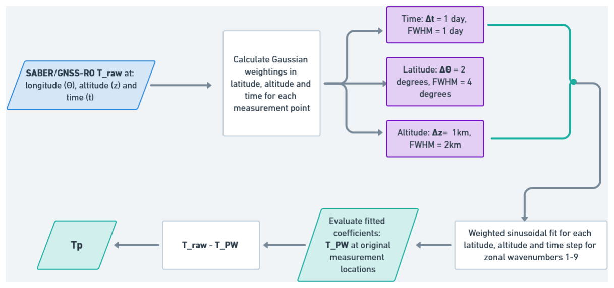
Figure 1A flowchart demonstrating the steps of the background removal method from the retrieved temperature data to the temperature residuals where the S-Transform is then applied to.
3.2 Definitions
Before we describe our main results, it is important to define some key terms that will be used extensively throughout the study.
Various studies on the QBO have chosen specific altitudes for their analysis, such as 30 km by Nath et al. (2014), ∼ 24 km (30 hPa) by Osprey et al. (2016), and 28 km by Ern et al. (2014). Given that the core of QBO variability occurs between 20 and 30 km, here we use the zonal wind from ERA5 data at 25 km over the latitudinal band of ±10° around the equator to define the QBO phases and cycles. A QBO cycle is defined in this study as the period corresponding to the distance between 2 successive eastward peaks of the zonal wind. The zonal wind is daily averaged and smoothed for the plot. The eastward (positive) and westward (negative) wind phases are referred to as the EQBO and WQBO phases, respectively, as shown in Fig. 2b.
The colour plot shown in Fig. 2c shows a time-height cross-section of an arbitrary QBO cycle with a period of 28 months. The time series plot shows the zonal wind at 25 km, with the positive part corresponding to the eastward phase of the QBO (EQBO) and the negative part corresponding to the westward phase (WQBO). The profile shown in Fig. 2a illustrates how we define the eastward and westward wind shears. The eastward wind shear is defined as the change of the wind with altitude from westward to eastward, and vice versa for the westward wind shear.
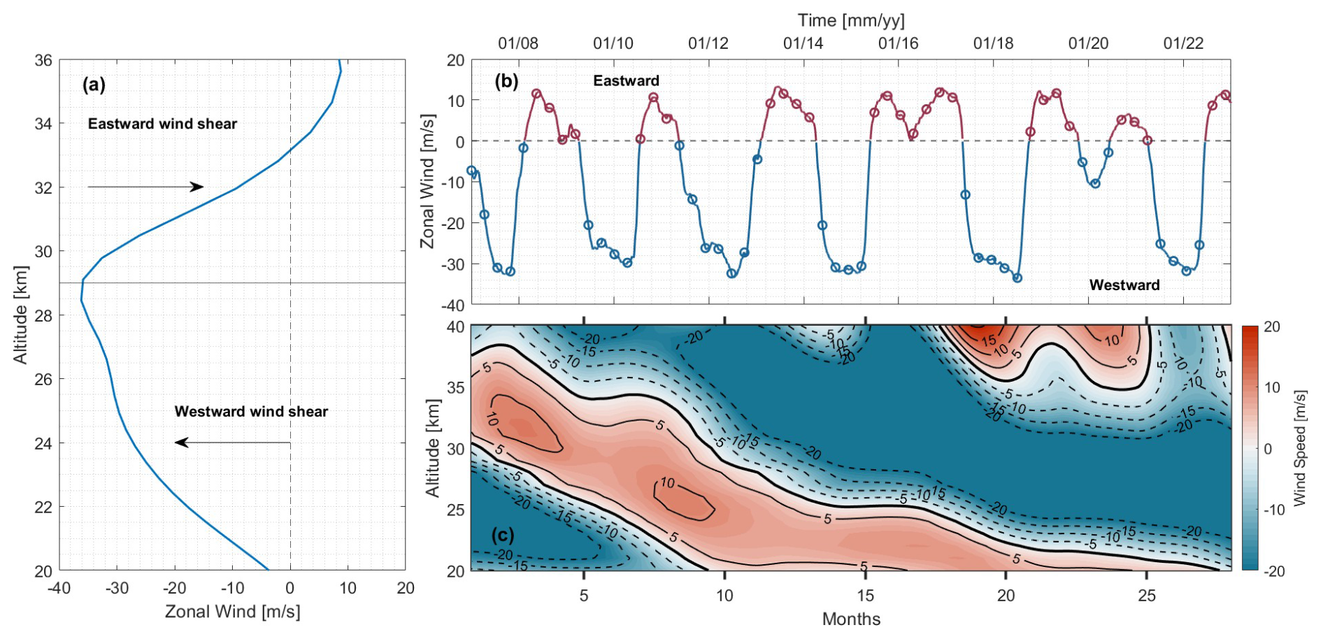
Figure 2Schematic representation of the QBO terminology through the study. Panel (a) shows the Eastward and Westward wind shear. Panel (b) shows the EQBO and WQBO, and Panel (c) is one arbitrary regular QBO cycle from the time series that shows the westward phase (blue) with the dashed contour lines and the eastward phase(red) with the solid contour lines. the thick black contour lines show the zero-wind line.
3.3 QBO cycles
The chosen period (2007–2022) encompasses five full QBO cycles. This period includes the only two disruptions recorded in more than 60 years of QBO data, specifically the major 2016 (e.g., Osprey et al., 2016) and 2019 (e.g., Anstey et al., 2022) disruptions. Since these two QBO disruptions are quite different in character, we consider each individually in our subsequent analyses. The first disruption is characterized by the QBO winds being westward above 30 km and eastward beneath. The westward phase propagated downward as is typical, but its descent had stalled. The second disruption in 2019 differs in that a shallow layer of westward wind appears between 25 and 30 km, interrupting the eastward phase.
Figure 3 shows the ERA5 zonal mean zonal winds in the tropics within the study period. We first divide the five cycles into two categories, specifically “regular” and “disrupted”. A “regular” cycle is a cycle of the period length of in average 28 months, while the disruptions are defined according to both literature as well as the cycles where a weakening of the eastward winds in the lower stratosphere occur interrupted by the westward wind (Osprey et al., 2016). Note that the regular QBO cycles vary in length and sometimes in structure. For example, the eastward wind shear is stronger at the end of 2009 indicated by the steep slope of zero-line wind, and the eastward wind is stalled at the beginning of 2009.
We compared ERA5 zonal winds to Singapore sonde winds and no significant differences are found between both datasets in their regions of vertical overlap. Based on this, we choose to use ERA5 for better coverage over the altitude ranges observed by GNSS-RO and SABER.
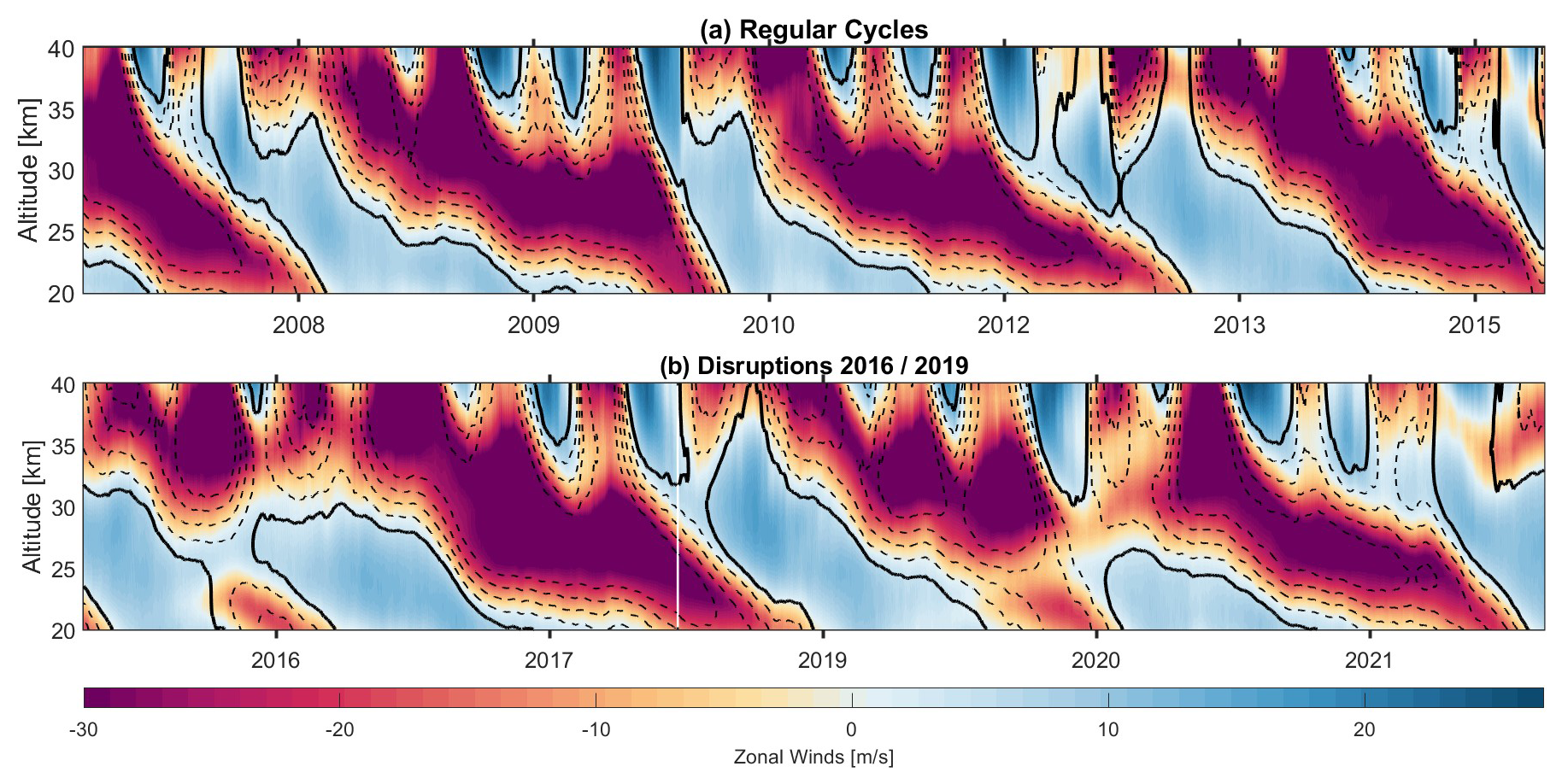
Figure 3Time-Height cross-section of the ERA5 zonal winds at the tropics for the period 2007–2022. Regular cycles (a) and the 2016 and 2019 QBO disruptions (b). The dashed contour lines and the purple colour represent the westward (negative) winds, the blue colour represents the eastward (positive) winds, and the solid lines indicate the zero-wind lines.
In this section, we compare both quantitatively and qualitatively the features of the GW signature derived from SABER and GNSS-RO observations. We carry out this comparison in terms of GW Ep and vertical wavelength λz; these two metrics are chosen because they can be measured easily using both instruments, unlike the other more heavily derived parameters such as momentum flux.
Before proceeding with analysis and comparison of both datasets, we first highlight the differences in observational filters between both instruments and how these differences may introduce discrepancies and biases in the results, potentially leading to the two instruments preferentially measuring different parts of the true geophysical GW spectrum. These main differences are:
-
SABER measures the atmospheric state along a regularly-spaced track, with a horizontal sampling spacing alternating between approximately 300–500 km between adjacent profiles at the height 30 km, arising as a result of the instrument's vertical scanning pattern (see e.g. Remsberg, 2008). In contrast, GNSS-RO provides profiles pseudorandomly located in both time and space, resulting in non-uniform coverage across different regions of the globe (Anthes et al., 2008). This difference in coverage leads to differences in the observed waves. For example, with SABER, we can estimate the horizontal wavelength (λh) of the wave given the distance between the adjacent profiles in time; however, accurate measurements of the λh are difficult or impossible for GNSS-RO because the profiles are not regularly spaced. It was possible to estimate the GW momentum flux (MF) and λh only at the early missions of GNSS-RO where the satellites were closely spaced, and this has been done in (e.g., Wang and Alexander, 2010; Faber et al., 2013), but this is not an option in the more general case we consider here.
-
Due to the nature of the instrument's temperature retrieval, the GNSS-RO measurements become increasingly dominated by a priori estimates of the atmospheric state with increasing height, making the data unreliable above about 40 km. However, below 40 km, GNSS-RO data maintains a high level of quality. In contrast, SABER data performs well in the 20–90 km altitude range but is less reliable at lower altitudes. Therefore, the most reliable range for comparison between these two datasets is from 20 to 40 km (Fan et al., 2015). This sensitivity to specific altitude ranges affects the estimation of the GW Ep from both instruments, with more reliability of GNSS-RO GW Ep results at lower altitudes than SABER and vice versa for higher altitudes (>40 km) (e.g. Wright et al., 2011, 2016).
-
SABER and GNSS-RO detect gravity waves differently due to their distinct geometries and line-of-sight (LOS) orientations relative to the wavefront. For GNSS-RO, any given wave is observed from a random direction, which can lead to amplitude degradation and phase shifts across individual profiles (Alexander et al., 2008). Since the LOS can intersect the wavefront at different angles, this results in apparent horizontal and vertical wavelengths that can differ from the true state, and wavelengths that can be distorted based on the relative orientation of the observation to the wave (Alexander et al., 2008). For SABER meanwhile, the latitude position of the measurement and orbital node from which the measurement is taken determines the angle from which each wave is observed, leading to a more consistent product with quite different direction biases to GNSS-RO, which can bias vertical wavelength and amplitude estimation (Trinh et al., 2015; Schmidt et al., 2016; Wright and Hindley, 2018).
-
GNSS-RO provides high vertical resolution, due to the precise bending angle measurement, allowing for measuring waves within the range (Wright et al., 2016). The horizontal resolution is also high, typically on the order of tens of kilometers ), due to the large number of GPS satellites and the wide distribution of receiving stations (Wright et al., 2011, 2016; Wright and Hindley, 2018). SABER on the other hand provides longer wavelengths and .
Given such differences, we expect GW properties measured by these two instruments to deviate from one another. To compare them as fairly as possible, in this study we use the same analysis method on both datasets and in doing so limit the analysis to GWs with vertical wavelengths ≤ 12 km. In subsequent Sections, we will compare SABER and GNSS-RO measured GW parameters first using a simple periodogram analysis, after which we will compare GW Ep and λz estimated from both instruments during different QBO cycles.
4.1 Periodogram
We first present results from a periodogram analysis of GW Ep derived from GNSS-RO and SABER data and ERA5 zonal winds, focusing on the tropics at an altitude of 25 km. We used the Lomb-Scargle periodogram analysis to detect and characterize the periodicity in each of the three time-series.
To permit a simple visual comparison, in our analysis we scale the power spectra resulting from this analysis to twice the total variance of each dataset for comparability. Figure 4 shows the resulting scaled periodogram, with the ordinate representing the scaled power spectra and the abscissa the periods of the inferred signals. Two scenarios were analyzed: the first covers the period without disruptions, from 2007 to 2015 (panel (a) of Fig. 4), and the second includes the disruption period, spanning from 2007 to 2022 (panel (b) of Fig. 4).
Figure 4a shows in black the periodogram measured for ERA5 zonal winds in the QBO region during the time where only regular cycles appear (corresponding to the periods shown in Fig. 3a). Periodograms derived from GW Ep as observed by GNSS-RO and SABER are overlaid in red and blue respectively. The dominant peak in the zonal wind data occurs at 2.44 years (approximately 29.35 months), which is slightly longer than the typical QBO cycle period of about 28 months. This peak is 6 times larger than the second-highest peak, indicating that the primary temporal characteristic of the zonal wind dataset is an oscillation with an average period of roughly 29 months. The peak does not align exactly with 28 months due to the irregularity of QBO cycles, which can extend beyond 28 months, and due to the short length of our data record relative to the long-term variability of the QBO.
The periodogram of GW Ep from SABER (blue line) exhibits two prominent peaks: a primary peak at a period of 1 year and a secondary peak corresponding to the typical QBO period. The primary peak indicates an annual variability in SABER GW Ep, consistent with earlier findings where gravity waves exhibited strong annual periodicity (Preusse et al., 2009; Zhang et al., 2012; Shuai et al., 2014). The secondary peak at 2.44 years confirms that SABER GW Ep is modulated by the QBO, aligning with previous studies such as Ern et al. (2014), which demonstrated that GW momentum flux with short vertical wavelengths (λz≤12 km) interacts with the QBO. The annual peak is more dominant than the QBO peak, even when focusing on short vertical wavelengths. This indicates that the GW spectra captured by SABER is dominated by a strong annual cycle rather than by interactions with the QBO.
The periodogram of GW Ep derived from GNSS-RO data presents a different pattern than SABER, featuring a broad primary peak at 2.72 years (around 32 months) and a smaller secondary peak at 1.25 years. The primary peak aligns closely with the zonal wind peak, while the annual peak reflects the seasonal variation of GW Ep. The 1.25-year peak remains unclear, though it may be related to shorter QBO cycles, which will be explored later.
The peaks and the shape of the periodogram changed when selecting longer period. This is true of all three datasets as shown in Fig. 4b. The reduced power of zonal winds is a mathematical consequence of the additional periodicity introduced by the disruptions, which occurs with periods over 28–29 months. While the dominant peak from the ERA5 zonal wind remains unchanged, a second peak of nearly equal power appears at approximately 2.92 years (≃ 34.6 months). Additionally, there is a third peak at 3.6 years (≃ 43.2 months) and two double peaks of equal power at 1.8 and 2 years. This variability can be partly explained by changes in the apparent length of the QBO periods during these disruptions. This result indicates that the time series of the zonal wind exhibits a superposition of short periods of 1.8–2 years and a longer period of approx. 2.3 years, as well as a longer period of the disruptions which is about 3.6 years.
Although the GW Ep from SABER shows a similar overall structure to the ERA5 zonal wind periodogram, the dominant peak remains at 1 year, with stronger power spectra compared to Panel (a). The second most prominent peak aligns with the regular cycle of the QBO. This confirms that the primary feature of the GW spectra observed by SABER is its annual variability, reflecting a pronounced seasonal cycle in the GW energy.
The GW Ep from GNSS-RO shifts with the change in analysis period to include the disruptions, now showing a dominant peak at 3 years (36 months), which remains stronger than the annual peak. The increased power at around 3 years suggests a stronger interaction between GW spectra captured by GNSS-RO and the QBO.
A persistent peak at 1.25 years is evident in all three datasets, suggesting a strong interaction between gravity waves (GW) and the quasi-biennial oscillation (QBO) in both SABER and GNSS-RO data. In zonal wind, the peak at 1.25 is not as strong as the peaks at 1.8 and 2 years, however, it is visible in the three datasets; ERA5 zonal winds, GNSS-RO, and SABER GW Ep. This is possibly due to the fact that zonal wind during the disruption apparently exhibits connected short periods of the QBO with a length of approximately 1.25 years. Statistical significance has been estimated for the primary peak of each of the three time series using the False Alarm Probability (FAP) technique. This approach estimates the likelihood of an incorrect finding in an analysis period. FAPs below 0.01 (1 %) are considered very secure. We estimated the values for all three parameters; QBO, Ep (GNSS), and Ep (SABER), finding that:
-
The most significant period of QBO is 2.4 years with 0 FAP.
-
The most significant period of Ep(GNSS) is 2.7 years with a FAP value of much less than a sensible number.
-
The most significant period of Ep(SABER) is 1 year with FAP of .
These values of FAP confirm that the dominant peaks of zonal wind, Ep from GNSS-RO and SABER are statistically significant.
It is well known that small-scale gravity waves contribute to the disruption of the QBO (Li et al., 2023). This periodogram analysis suggests that GNSS-RO, with its higher sensitivity to shorter vertical wavelengths, finer vertical resolution, and broader altitude coverage, captures these small-scale waves and their effects more effectively. In contrast, SABER is more sensitive to longer wavelengths, perhaps leading to undersampling of the shorter scales. This difference may explain why the effect of the two disrupted QBOs is clearly visible in the periodogram of GW Ep from GNSS-RO but not as distinctly in the SABER data. The results further suggest that the ability of GNSS-RO to capture gravity wave spectrum changes linked to the QBO better than SABER may mainly be due to differences in their respective observational filter.
Although the periodogram method is highly sensitive to the length and variability of the input data, it remains a valid approach that confirms previous findings about small-scale GWs playing a major role in driving the QBO (e.g., Wang and Alexander, 2010; Anstey et al., 2022; Nath et al., 2014; Tsuda et al., 2011). Instruments with longer vertical wavelengths, such as AIRS data, for example, do not show any QBO signal (Hindley et al., 2019a). These results underscore the importance of comparisons between SABER and GNSS-RO as a means of highlighting the instrument's relative sensitivity to different scales of gravity waves and of identifying the influence of their observational filters in capturing GW-QBO interaction.
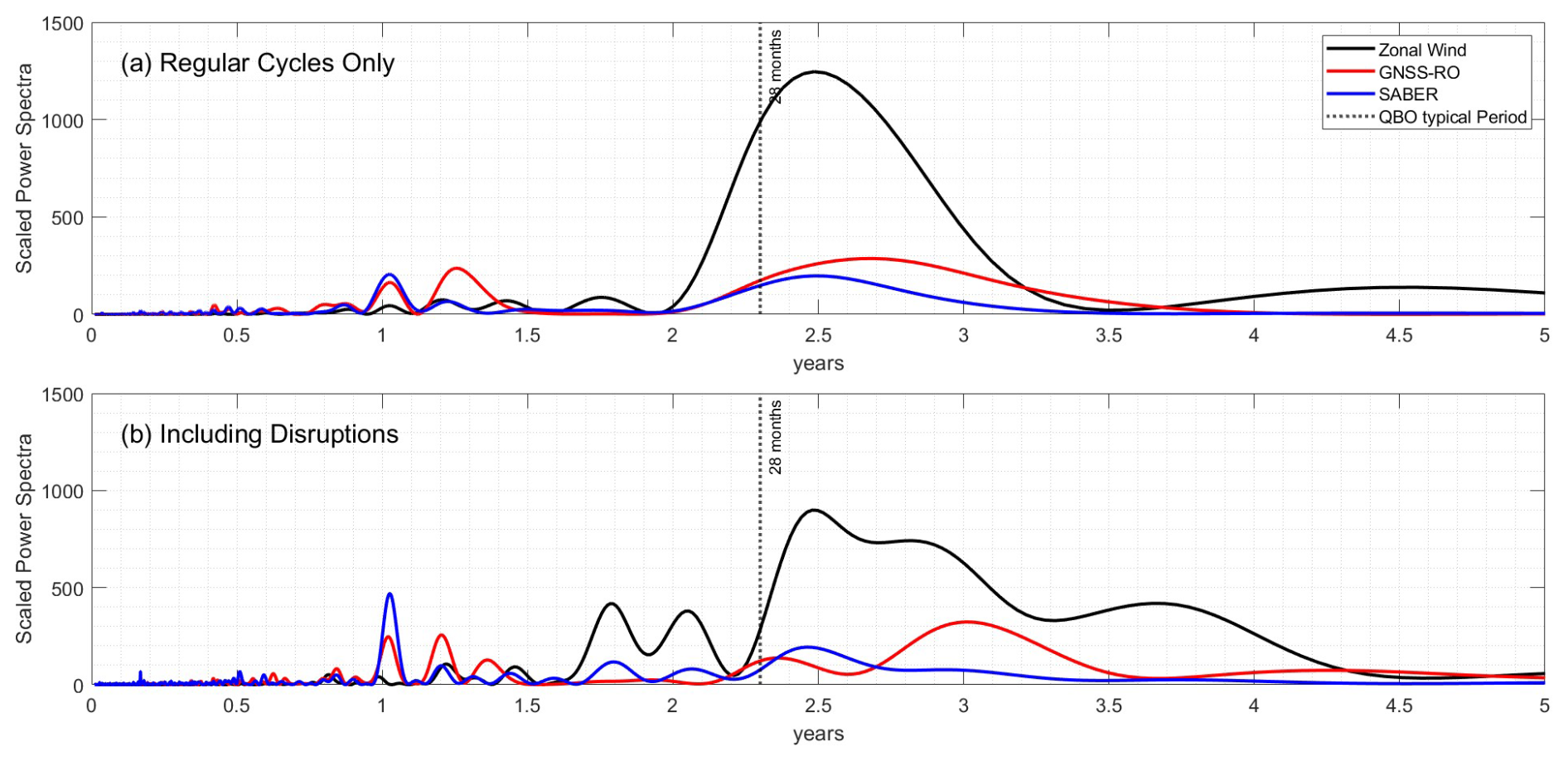
Figure 4Periodogram of the ERA5 zonal mean zonal winds (black), GW Ep from GNSS-RO (red), and SABER (blue). The theoretical period of the QBO is indicated by the dashed line. Panel (a) is the period from 2007 to 2015, where no disruption occurs, and panel (b) is for the whole period (2007–2022), including 2016 and 2019 disruptions. The x-axis is the time in years. the y-axis is the scaled power spectral density.
4.2 Potential Energy from GNSS-RO and SABER
We next proceed to examine the key differences between GNSS-RO and SABER in capturing the GWs-QBO interaction. Specifically, in this section we examine the difference in GW Ep measured by the two instruments, and how this is modulated by the QBO.
Figure 5 shows the GW Ep difference between GNSS-RO and SABER averaged over the latitudes ±10° during different QBO cycles. The absolute values of Ep and λz for each instrument are shown in the Figs. A1 and A2, respectively. For simplicity, and since the GW Ep from both instruments does not vary significantly from one regular QBO cycle to another, we chose to focus on the first regular QBO cycle within the study period as a representative example of the three regular cycles. In contrast, the 2016 and 2019 disruptions are presented separately due to their distinct characteristics. Our results exhibit several key features:
-
GNSS-RO exhibits higher GW Ep than SABER in all cycles, as shown by Fig. 5a. This difference is on average of order 2 J kg−1 and reaches a maximum of 5 J kg−1 at lower altitudes (20–25 km). The difference decreases with altitude until it almost vanishes at altitudes above 35 km.
-
The most evident dissimilarity in GW Ep is found at lower altitudes and during the transitions between QBO phases, such as from EQBO to WQBO and vice versa. This is attributed to the varying sensitivity of each instrument to specific altitude ranges (Tsuda et al., 2009; Ern et al., 2018). The GNSS-RO exhibits higher Ep at the phase transitions and during the eastward phase because of the variation of the GW convective sources around the equator at the northern and southern hemispheres. This is in agreement with previous studies showing that most of the GW activity is found at the transitions between QBO phases and due to the inter-hemispheric variability e.g., (De la Torre et al., 2006; Nath et al., 2014; Luo et al., 2021).
-
During the 2016 disruption, the GW Ep difference between GNSS-RO and SABER is smaller above ∼ 30 km compared to the other two cycles and even reverses at an altitude of around 34 km, where GW Ep from SABER slightly larger than that of GNSS-RO.
-
The difference is smaller during the WQBO phase. Notably, GW Ep tends to diminish or be filtered out, particularly from SABER, above the zero-wind line. This is consistent with previous findings by Ern et al. (2014).
-
During the 2016 disruption, the difference is minimal above 30 km. This is possibly due to the decreased GW activity during the disruption (Luo et al., 2021; Li et al., 2023).
-
The pattern of Ep during the 2019 disruption closely matches that of the 2016 disruption, with an increase in GW Ep observed during the transition from the eastward to the westward phase of the QBO. Overall, GNSS-RO shows higher Ep at all altitudes than SABER during the 2019 disruption compared to the 2016 event.
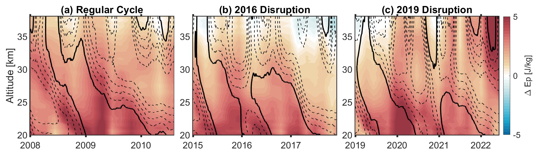
Figure 5Time-Height cross-section of the difference in GW Ep between GNSS-RO and SABER (color map) overlaid by the zonal winds at the QBO region shown in contour lines, with solid lines represent zero-wind line and dashed lines represent the westward winds with a spacing of 5 m s−1 during one regular cycle (a) the 2016 disruption (b) and the 2019 disruption (c).
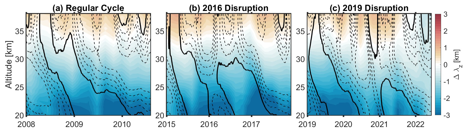
4.3 Vertical wavelength from GNSS-RO and SABER
Next, we investigate how the observational filters of each instrument affect the vertical wavelength of the observed gravity waves.
During “typical” QBO cycles, both GNSS-RO and SABER display a consistent pattern of longer vertical wavelengths at higher altitudes and shorter ones at lower altitudes. This is consistent with our understanding of GW propagation, as shorter vertical wavelengths are typically filtered out by the wind at lower altitudes, while larger vertical wavelengths are less affected by dissipation and, therefore, tend to propagate higher (e.g., Yiğit and Medvedev, 2016; Heale et al., 2018). Notably, during the three QBO cases, vertical wavelength from GNSS-RO is minimum at the transitions from EQBO to WQBO and vice versa except at the end of the 2019 disruption. This trend is not observed in SABER.
When we identified discrepancies between our results from SABER and GNSS-RO, we ascribed these differences to the limitations in each instrument's observational filter in Sect. 4. However, the exact causes behind these variations remain unclear – in particular, which specific elements of the observational filters contribute to these differences? In this section, we investigate the factors driving these discrepancies, to link them to measurable parameters. Additionally, we aim to gain a better understanding of how different the observational filters are of these two instruments. Addressing these differences is crucial to determining whether GNSS-RO data can be used to extend the study of GW-QBO interactions, building upon the extensive previous work using SABER.
To do this, we use one week of output (representing the period 20–26 January 2020) from a 40 d free-running DYAMOND-WINTER simulation carried out using the 3 km resolution GEOS model. These dates were selected as they are close to model initialisation on the 20 January, and thus represent a broadly realistic atmospheric state. Using this model output, we produce synthetic estimates of temperatures in the model as they would be observed by SABER- and GNSS-RO-type instruments. The high resolution of the GEOS model allows it to capture a large fraction of small-scale gravity waves (Holt et al., 2016, 2017). The model is capable of reproducing a realistic QBO in Holt et al. (2016), making it an appropriate choice for our study.
In Sect. 4, we discussed the observational filter differences between SABER and GNSS-RO. To identify the key factors contributing to the discrepancies in GW Ep results between the two instruments, we here sample GEOS temperatures to simulate the temperature retrievals of SABER and GNSS-RO, following the method from Wright and Hindley (2018), which has previously been applied to reanalysis data (Wright and Hindley, 2018) and to high-resolution global model data (Lear et al., 2024).
Using this approach, temperature estimates were extracted from the model and used to compute GW Ep and λz, at resolutions and oversampling volumes consistent with true SABER and GNSS-RO measurements. To derive gravity wave parameters, we then applied the same background removal technique as used for the actual SABER and GNSS-RO temperature data in Sect. 3.1, followed by applying a second-order Savitzky-Golay low-pass filter with a 3 km frame size to smooth out small-scale variations. This approach is similar to the method described in Hindley et al. (2015). Here we used the Savitzky-Golay filter instead of the weighted sine fitting approach (Sect. 3.1) because the data length was insufficient for the sine fitting method. Finally, we applied the S-Transform to the temperature perturbations T′ to extract the vertical wavelength λz and then used Eq. (1) to calculate GW Ep. The range of the vertical wavelength used for sampling both instruments is between 2 and 14 km.
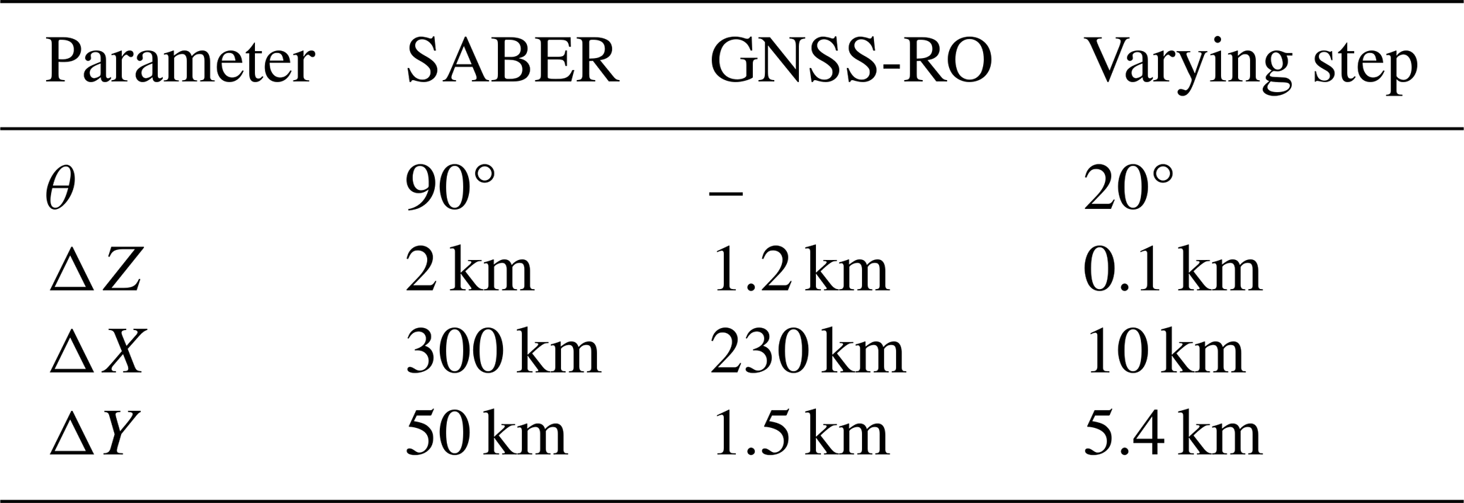
To understand the differences between the two instruments, we then systematically varied four key parameters representing differences between measurements made by the two real instruments and used the resulting data to assess the impact of these varied parameters on “measured” GW Ep. The four parameters, varied over the ranges described in Table 1, are defined as follows:
-
Viewing Angle (θ): this is defined as the bearing between the north and the instrument Line-Of-Sight (LOS). For SABER, this angle alternates between 90° off the satellite's along-track travel vector for the northward-looking mode and 270° for the southward-looking mode (Trinh et al., 2015). Real GNSS-RO data have a randomly distributed viewing angle due to their varying orientations.
-
Vertical resolution (ΔZ): This is defined as the FWHM of the vertical averaging implicit in the combined measurement and retrieval of each instrument, and represents the minimum altitude separation at which two atmospheric features can be distinguished in the retrieved profiles.
-
For GNSS-RO, the vertical resolution depends on the bending angle; more information about the determination of vertical resolution of GNSS-RO data can be found in Kursinski et al. (1997).
-
For SABER, the vertical resolution is determined by the projection of the field of view (Mertens et al., 2009).
-
-
Along-LOS resolution (ΔX): This is defined as the FWHM of the instrument's resolution along the Line-Of-Sight (LOS) (Wright and Hindley, 2018), we will refer to it as “aLOS” in the following text:
-
For GNSS-RO, Kursinski et al. (1997) defines the aLOS resolution (ΔZ) as the distance traveled by the GPS ray as it enters and exits the atmosphere, approximately 270 km.
-
For SABER, aLOS is determined by the instrument's Field-Of-View (FOV), detector size, and the satellite's velocity (Wu et al., 2006; Trinh et al., 2015), and it is on average 400 km (Alexander et al., 2008).
-
-
Across-LOS resolution (ΔY): This is defined as the FWHM of the instrument's resolution across the LOS. This refers to the resolution in the direction perpendicular to the satellite's flight path, affecting the ability to resolve features across the satellite's swath or footprint. This parameter is crucial in remote sensing, as it determines the instrument's capability to capture features across the satellite's motion. We will refer to this parameter as xLOS.
Table 1 presents the different values selected for each of the four parameters, based on the characteristics of SABER and GNSS-RO. The viewing angle was varied from −90 to 70° in 20° increments, with higher angles excluded to prevent the repetition of the same angles for the selected profiles (Wright and Hindley, 2018). The vertical resolution was varied from 1.2 to 2 km, in steps of 0.1 km, representing the resolutions of GNSS-RO and SABER, respectively. The aLOS resolution was varied from 230 to 310 km in 10 km steps, while the xLOS resolution ranged from 1.2 to 50 km, with a step size of 5.4 km. We systematically vary each parameter within its defined range and run our sampling code at each specific value. This process provides the sampled temperature corresponding to each value for each parameter, while keeping the other parameters fixed as each individual parameter is varied.
Table 1Varied parameters for the model sampled data with the value of each parameter corresponding to each instrument and the varying step. θ: viewing angle, ΔZ: Vertical resolution, ΔX: along-LOS resolution, ΔY: across-LOS resolution.
5.1 Results
5.1.1 Gravity Wave Potential Energy
Figure 7 presents the model-sampled GW Ep for SABER (grey) and GNSS-RO (pink). Each panel corresponds to one of the four studied parameters. The mean GW Ep between 20 and 30 km altitude for each instrument is displayed over the 1-week simulation period, illustrating how it varies across the range of tested parameter values. The dark-shaded regions represent a 50 % confidence interval derived from a bootstrap analysis with 10 000 resamplings, while the lighter-shaded areas indicate a 95 % confidence interval. It is important to note that the mean shown here is the median of the bootstrap-estimated distribution of mean states. The results show the following:
-
Viewing angle:
In general, the GW Ep from the sampled GNSS-RO is roughly twice as high as that from the SABER-sampled GW Ep. For GNSS-RO, the variation in Ep with respect to the viewing angle is well within our uncertainty range, consistent with the true observations being randomly distributed in the viewing angle; specifically, the change in Ep across different angles is around 0.5 J kg−1, indicating a negligible impact. For SABER, during this period, the TIMED satellite faced northward. Since it is inclined by 74.1° with respect to the true north, the viewing angle should be . Ep shows a minimum around 10°, with a slight variation of approximately 0.1 J kg−1 between the minimum and maximum values across angles. This suggests that changes in the viewing angle do not significantly affect Ep for either SABER or GNSS-RO.
-
Vertical Resolution:
Both GNSS-RO and SABER exhibit similar behavior in terms of vertical resolution. The GNSS-RO vertical resolution is 1.2 km, while for SABER it is 2 km. The GW Ep in both instruments decreases significantly, compared to other parameters, when transitioning from higher to lower resolution. As vertical resolution improves, the GW Ep increases, capturing a larger portion of the gravity wave spectrum, particularly small-scale waves. The difference in GW Ep between SABER and GNSS-RO is around 2 J kg−1, and this discrepancy is consistent across both instruments. This finding underscores the important role that the vertical resolution plays in estimating GW Ep. Additionally, the narrow 50 % and 95 % confidence intervals for both instruments suggest that the mean GW Ep and its variation with vertical resolution (ΔZ) reliably reflect the impact of resolution on GW Ep values.
-
aLOS Resolution:
The offset between GW Ep from SABER and GNSS-RO remains, with GW Ep from GNSS-RO being approximately twice as large as that from SABER. The impact of aLOS variation on GW Ep is even smaller than the effect of viewing angle. For GNSS-RO, the variation is around 0.2 J kg−1, while for SABER it is less than 0.1 J kg−1.
-
xLOS Resolution:
GNSS-RO exhibits a very slight variation in GW Ep with changes in xLOS resolution. Conversely, SABER shows no variation in GW Ep with changes in ΔY. The large uncertainty surrounding the mean in both ΔX and ΔY plots indicates that the impact of these parameters on the variability of GW Ep is not significant or clearly defined.
It is important to highlight that these analyses examine only one week of data from a free-running model which is inherently limited in resolution relative to the true atmosphere, albeit high relative to most current global modelling.
The offset of 2 J kg−1 between SABER and GNSS-RO that is seen for all the parameters, except in the vertical resolution, is in agreement with the observations as shown in Sect. 4. This is a good indication that our experiment maintains a geophysically-plausible results.
From the results, it is shown that the vertical resolution plays a major role in the variation of GW Ep for both SABER and GNSS-RO. By increasing the vertical resolution, the GW Ep increased by almost twice the value. This suggests that the offset of the double value of Ep between SABER and GNSS-RO is almost entirely caused by the vertical resolution. We will test this hypothesis in Sect. 6 using the real observations from both instruments.
5.1.2 Vertical Wavelength
Figure 8 shows the distribution of the measured vertical wavelength against each parameter for GNSS-RO (upper panels) and SABER (lower panels), again averaged over the altitudes 20–30 km. The distributions are shown as densities using a normal kernel density function; probability-density functions have also been tested and show similar results but with much larger noise levels. The ordinate of the kernel density is scaled such that the total area under the density is 1, where the area represents the probability with continuous distributions.
-
GNSS-RO: The distribution of λz is nearly identical across all four parameters, displaying a bimodal shape with two peaks: one at 6.7 km and another at 8 km. The 8 km peak is slightly more pronounced. This result aligns with the vertical wavelength distribution presented in Fig. 6 of Hindley et al. (2015), though with slightly higher values in the latter study due to the wavelength selection constraints we applied. The variability among the curves reflects changes in the distribution for each parameter, but this variability is minimal, indicating that the GW Ep remains relatively consistent despite changes in the parameters. The greatest variability between peaks occurs for vertical resolution, with longer λz becoming more dominant when the vertical resolution is varying.
-
SABER: The distribution of vertical wavelengths for SABER differs from that of GNSS-RO, showing a nearly normal distribution around 8 km across all parameters, except for vertical resolution. SABER distributions also show a more pronounced tail to smaller wavelengths than GNSS-RO. The longer dominant vertical wavelength in SABER compared to GNSS-RO aligns with the results from our analysis as well as from previous studies (Wright et al., 2016). The variation in viewing angle also influences the distribution of λz, as anticipated, given the geometry's impact on detecting different wavelengths (Trinh et al., 2015). Changes in viewing angle can cause the satellite's line of sight to intersect the atmosphere at different altitudes, affecting the observed vertical wavelengths of gravity waves, as noted in studies like (Wu et al., 2006; Ern et al., 2018).
To quantify the variation of λz with each parameter, we examine the variation of the mean λz with the variation of the values of each of the four parameters as shown in Fig. 9. Again we show the median value of the bootstrap distribution of means for this analysis. The results show that:
-
In general, for all the four parameters, SABER displayed longer λz than GNSS-RO. This agrees with the results shown from the observations as shown in Sect. 6.
-
In SABER, the vertical wavelength slightly changes with the viewing angle. However, this variability is small, on the order of 0.5 km. GNSS-RO on the other hand displayed nearly no change in vertical wavelength with θ. This is reasonable since SABER is observing from a fixed angle while GNSS-RO observes the wave from various angles.
-
Vertical resolution is the most important parameter for determining the measured vertical wavelength. For GNSS-RO the relation between the vertical wavelength and the vertical resolution is almost linear, i.e., the coarser the vertical resolution, the longer the vertical wavelength detected by the instrument. This is not the case for SABER, where varying the vertical resolution does not strongly impact the measured vertical wavelength. This assures the previous results that shown in Fig. 8a, b, and c that a combination of the three parameters most probably influences the vertical wavelength detected by SABER; θ,ΔZ, and ΔX.
-
aLOS and xLOS resolutions have almost no effect on the vertical wavelength, particularly for GNSS-RO. For SABER, aLOS has a slight influence on vertical wavelength detection. Since the wave fronts in the model are inclined relative to the instrument's horizontal and vertical detection axes, the horizontal sampling distance can influence the estimation of vertical wavelength. For instruments with a longer horizontal sampling range, the averaging differs slightly compared to those with shorter ranges, introducing aliasing. This causes a tendency toward detecting longer λz with greater horizontal sampling distances, as seen with SABER, and shorter λz with shorter horizontal distances, as with GNSS-RO.
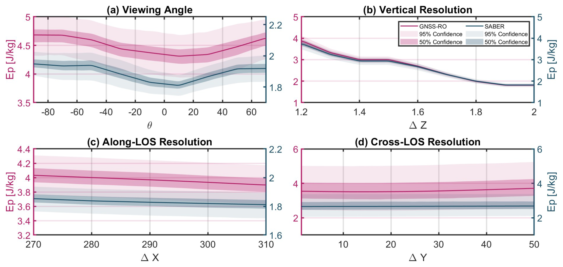
Figure 7The variation of the model-sampled bootstrap mean of GW Ep with respect to the four parameters: θ (a), ΔZ (b), ΔX (c), and ΔY (d). The darker shading represents the 50 % and the lighter shading indicates the 95 % confidence intervals around the mean.
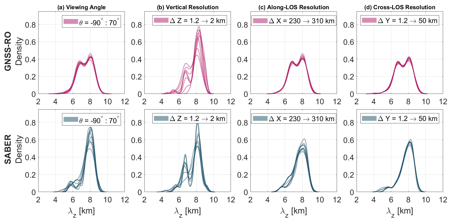
Figure 8Kernel density of λz distributions at different parameters; θ (a), ΔZ (b), ΔX (c), and ΔY (d) for GNSS-RO (upper row) and SABER (lower row). The legend indicates the range of the values for each of the four parameters.
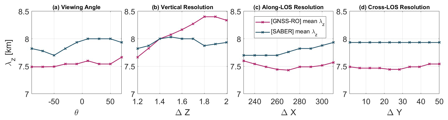
Figure 9Median λz varied with four parameters; θ (a), ΔZ (b), ΔX (c), and ΔY (d) shown for GNSS-RO (pink) and SABER (blue).
As demonstrated above, the difference in vertical resolution between SABER and GNSS-RO is the primary factor responsible for the discrepancies in the GW properties they measure in the QBO-dominated tropical lower stratosphere, particularly when considering GW Ep. In this section, we build on this finding to explore how the observations can be considered in a more equivalent way for future work.
We analyzed the GEOS model temperatures sampled as GNSS-RO and SABER retrieved temperatures. Our results identified the vertical resolution as the most crucial factor contributing to the differences in Ep and λz. Based on these results, we then adjusted the GNSS-RO observations to match SABER's vertical resolution. We apply a boxcar smoothing to the raw GNSS-RO temperature profiles with an interval of 2 km in altitude before performing the GW analysis. Initially, the GNSS-RO temperature data had a resolution of 1.2 km. We then applied the method described in Sect. 3.1 to the smoothed temperatures to extract gravity wave properties.
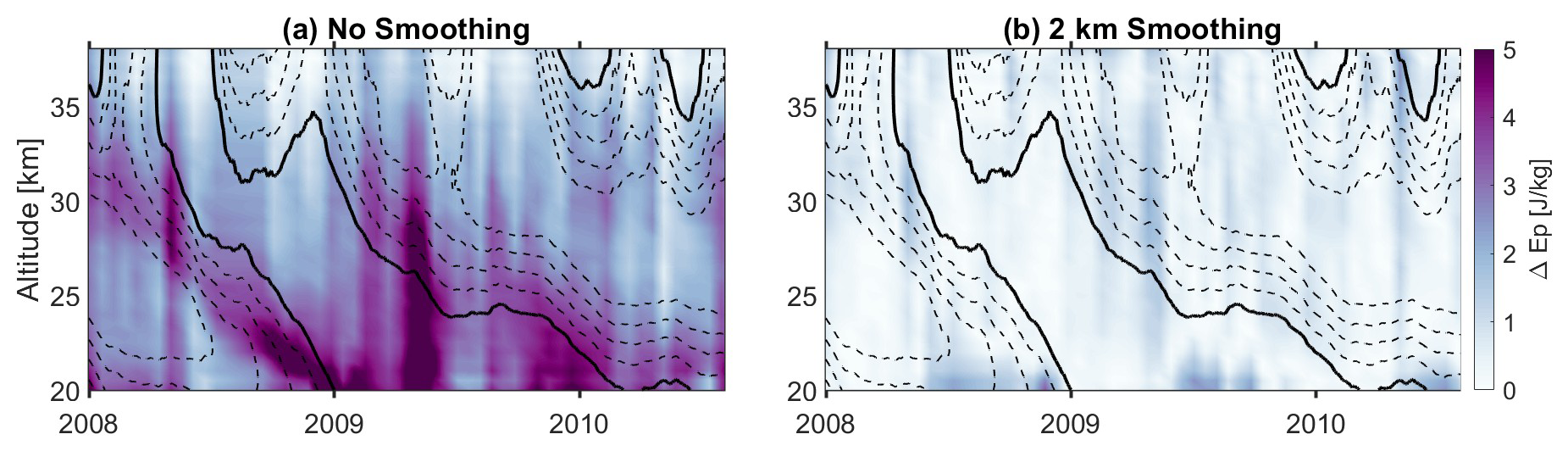
Figure 10Time-height cross-section of the absolute difference in Ep between GNSS-RO and SABER during an arbitrary regular QBO cycle as shown by the color map, overlaid by the contour lines of the zonal winds. solid lines are the zero-wind line and dashed lines are westward winds with a spacing of 5 m s−1. Panel (a) shows the difference in Ep before applying a 2 km boxcar smoothing to the raw GNSS-RO temperature profiles with an interval of 2 km in altitude and panel (b) shows the difference after the 2 km smoothing.
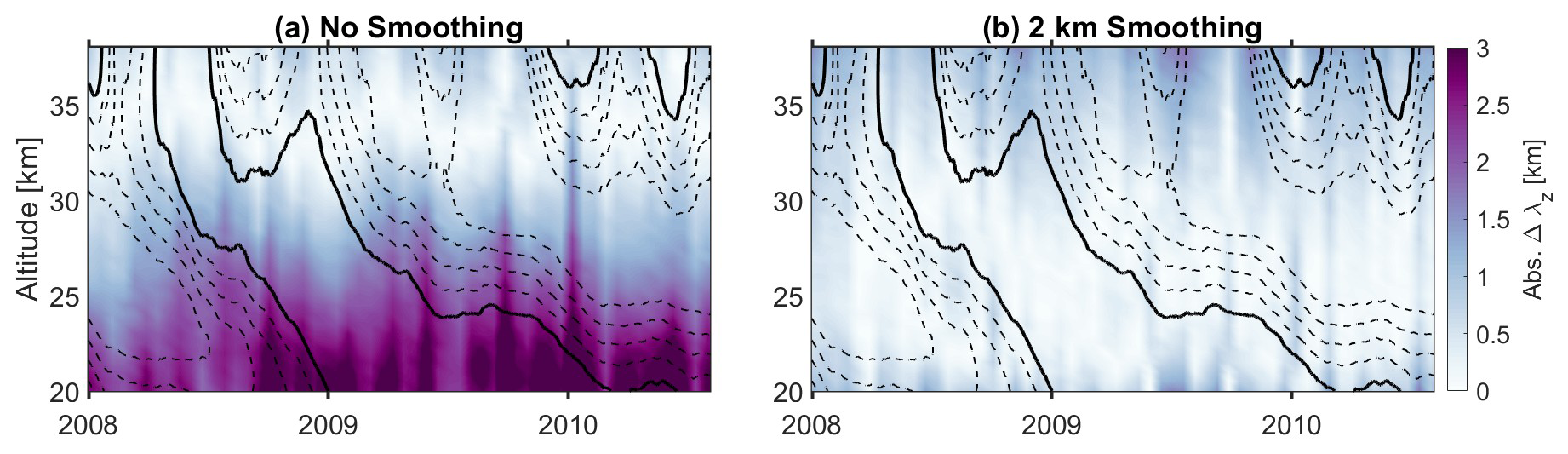
Next, we recreated Figs. 5 and 6 using the Ep estimation from the smoothed GNSS-RO temperatures for a given regular QBO cycle. Figures 10 and 11 show the resulting absolute differences in GW Ep and λz, respectively, with the left panels showing results before and the right panels after smoothing GNSS-RO temperatures.
6.1 GW Ep
After smoothing, the largest differences are observed in regions where the GNSS-RO GW Ep was initially much higher than that of SABER, particularly in areas where the Ep difference exceeded 5 J kg−1 (Fig. 10a). This mainly occurs within the eastward wind shear during the QBO's eastward phase at lower altitudes and at the transition from the EQBO to the WQBO phase. Post-smoothing, these discrepancies are significantly reduced to approximately , consistent across all altitudes and during all QBO phase transitions.
6.2 Vertical Wavelength λz
The impact of smoothing on vertical wavelength differs from its effect on Ep. The difference in vertical wavelengths decreases at some altitudes and reverses at others. Before smoothing, GNSS-RO consistently detected shorter vertical wavelengths than SABER. After smoothing, GNSS-RO wavelengths become longer than those of SABER below approximately 22 km and above around 29 km. Between 22 and 29 km, the vertical wavelengths from both instruments are nearly identical, with GNSS-RO showing slightly shorter wavelengths than SABER. This is consistent with the model-sampled data discussed in Sect. 5.1.2, which showed that the relationship between λz and vertical resolution for SABER is not linear, suggesting the influence of additional factors.
These findings, along with the model data, suggest that factors beyond vertical resolution, such as a variation or a combination of variation viewing angle, and vertical and aLOS resolutions, are contributing to the change in vertical wavelength detection. To quantify this combined effect, we normalized the vertical wavelength variations with respect to each of the three parameters – θ, ΔZ, and ΔX – to a range between 0 and 1. We then calculated the mean λz variation for each parameter and summed these values to represent the total variation in λz. Finally, we determined the contribution of each parameter to the total variation by calculating the ratio of the individual means to the total. The results showed that θ accounts for 32 % of the total variation, ΔZ contributes 36 %, and ΔX contributes 32 %.
6.3 Time series and Distribution
In this section, we analyze the time series and the distribution of Ep from both GNSS-RO and SABER before and after applying a 2 km smoothing to the GNSS-RO temperature data. We investigate the ability of GNSS-RO to extend the climatology of SABER. This can be achieved by comparing the time series of Ep throughout the SABER period and the smoothed GNSS-RO data at a selected height and examining how well the two time series are aligned. Figure 12 presents the time series of Ep at 30 km from SABER and GNSS-RO both before and after smoothing. The smoothing process significantly reduces the differences between the two data sets, quantitatively and qualitatively. The distribution of the GNSS-RO data has changed significantly. The two distributions, before and after smoothing GNSS-RO data, are statistically significantly different () on a non-parametric two-sample Kolmogorov-Smirnoff test. We use this test instead of Student's t-test as the distributions are non-Gaussian
The small discrepancy between smoothed GNSS-RO and SABER timeseries is influenced by data coverage and the number of available GNSS-RO missions. Before the late 2010s, when data availability is lower (see Fig. 2 in Leroy et al., 2023), the two time series are not well-aligned quantitatively. However, they still exhibited strong qualitative agreement, capturing high and low periods of Ep indicative of a strong QBO signal in both datasets. After 2010, the time series begin to align both quantitatively and qualitatively. Between 2015 and 2020, reduced data availability from the COSMIC-1 satellite (see Fig. 2 in Leroy et al., 2023) and insufficient data from other missions affected the accuracy of Ep calculations. This could also be due to the filtering of gravity waves by the QBO winds during the 2016 disruption, as shown in the reduced Ep in the period of 2016 to 2019 in Fig. 13. This is in agreement with what has been shown earlier in Fig. 5b. Post 2020, the launch of additional GNSS-RO missions with a significantly larger number of daily measurements (reaching up to 6000 profiles per day from COSMIC2 satellite) improved the estimates Ep. This will be explained in detail in the following paragraph. Overall, the two time series show strong qualitative agreement throughout the 16-year study period. Furthermore, after smoothing, the GNSS-RO Ep distribution closely matches the SABER distribution, with a peak around 5 J kg−1, compared to an initial peak of approximately 8 J kg−1 before smoothing. This result further confirms the feasibility of using GNSS-RO data to extend SABER observations.
Figure 13 presents Ep for each of the 12 individual radio occultation missions used in our study over the period 2007 to 2022. The figure shows a consistent pattern across all instruments, with a strong QBO signal, particularly between 2007 and 2018. A decline in Ep is noticeable around 2018, coinciding with the westward phase of the QBO following the 2016 disruption, as well as a reduction in the number of observations, as demonstrated by Leroy et al. (2023) in Fig. 2.
This figure provides evidence that all missions capture small-scale gravity waves interacting strongly with zonal winds in the QBO region. However, it also highlights quantitative differences in Ep estimates among missions. For instance, COSMIC-1 and MetOp, both operational since 2007, had slightly different observation counts until 2019, with COSMIC-1 providing more profiles. Despite this, COSMIC-1 show higher mean Ep values than MetOp. This suggests that merging RO missions, as in this study, leads to an accurate estimate of Ep.
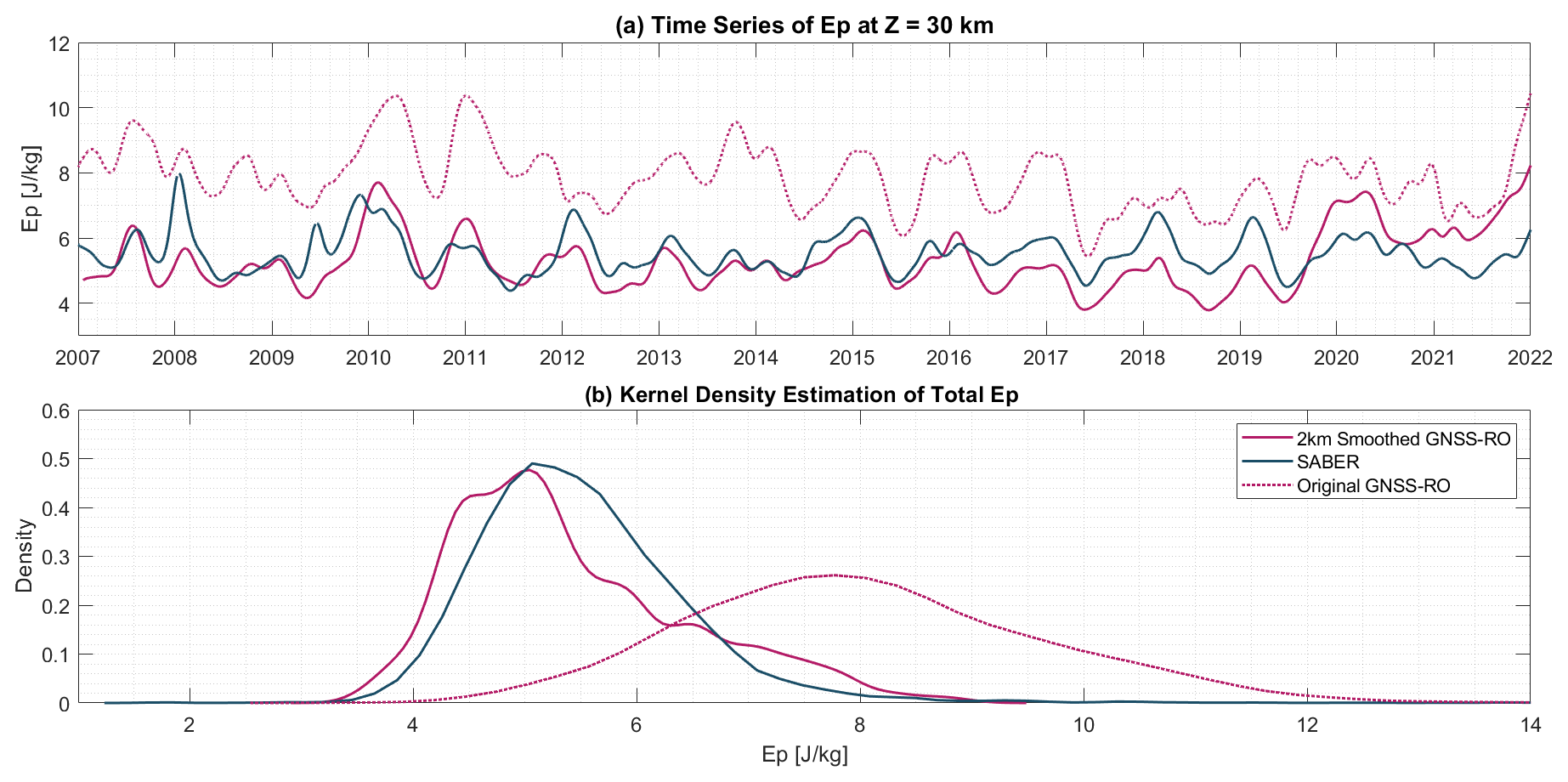
Figure 12Panel (a) shows the time series of Ep derived from 2 km boxcar smoothed GNSS-RO temperatures (solid pink), SABER actual temperatures (blue), original GNSS-RO temperatures (dashed pink) at an altitude of 30 km. Panel (b) shows the kernel density of the Ep distribution from the three datasets at all altitudes from 20–40 km.
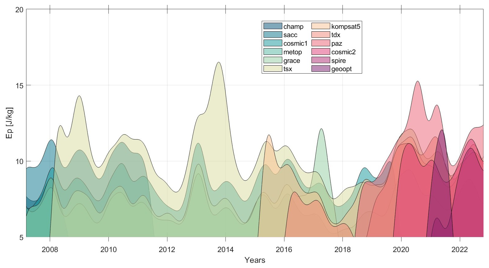
Figure 13The distribution of linearly interpolated gaussian smoothed Ep throughout the study period (2007–2022), as derived from each of the 12 individual radio occultation missions included in the merged GNSS-RO dataset. The area under each curve has been shaded to better distinguish the lines visually.
There are several key points in this study that we believe are important to highlight and discuss. First, the periodogram results in Sect. 4.1 showed that Ep from SABER remains stable regardless of the study period length, highlighting the consistent annual cycle present in SABER-derived GW time series. This annual cycle becomes more pronounced over longer periods of study, aligning with previous findings: for instance, John and Kumar (2012) showed a seasonal variation of Ep from SABER in the tropics, superimposed by the same periodicity of the regular QBO. It also confirms earlier findings by Ern et al. (2014) that the QBO modulates GW temperature amplitudes.
However, the variability in Ep observed from GNSS-RO depending on the length of the study period suggests a stronger modulation by the QBO. The dominant fluctuations in Ep from GNSS-RO coincide with QBO periods, particularly the disruption periods, implying that the QBO more strongly influences the gravity wave spectra observed by GNSS-RO. This agrees with earlier studies showing a pronounced QBO signal in GNSS-RO data (e.g., Namboothiri et al., 2008; Tsuda et al., 2009; Nath et al., 2014). This difference is likely driven by the ability of GNSS-RO to measure vertically-shorter waves.
Second, the comparison of Ep between SABER and GNSS-RO, as illustrated in Fig. 5, indicates that GNSS-RO consistently observes higher GW Ep than SABER, particularly at lower altitudes. This is due to GNSS-RO's stronger sensitivity to shorter spatial scales and lower altitudes, allowing it to capture a wider part of the gravity wave spectrum than SABER. This effect is evident in Fig. 6, where GNSS-RO exhibits shorter vertical wavelengths compared to SABER.
In summary, the main differences between GNSS-RO and SABER are:
-
The time series of Ep from GNSS-RO exhibits a dominant power spectral peak at the typical QBO cycle period (∼ 28 months), compared to the annual peak. In contrast, Ep from SABER shows a stronger annual peak compared to the QBO-related one. When accounting for disruptions, GNSS-RO exhibits a pronounced peak at a longer period than the regular QBO cycle, highlighting the influence of small-scale gravity waves captured by GNSS-RO in QBO disruptions.
-
GNSS-RO shows higher Ep than SABER in the QBO region, particularly at lower altitudes. We attribute this to a combination of the observational filter and the higher vertical resolution of GNSS-RO, enhancing its ability to capture small-scale gravity waves.
-
The model-sampled data as GNSS-RO and SABER temperature indicate that the primary factor driving differences in Ep and λz between the two measurements is the difference in their vertical resolution.
-
Ep results from both instruments exhibit a strong QBO signal during both regular and disruption periods.
-
The results of the model sampled GNSS-RO and SABER indicate that factors such as aLOS and xLOS have no impact on either Ep or λz.
-
GNSS-RO estimates of GW activity much more closely approximate those observed by SABER when the vertical resolution of the GNSS-RO data is degraded to approximate that of SABER.
This outcome aligns with previous studies. For instance, Tsuda et al. (2009) found that GPS RO data consistently showed maximum Ep in the tropics within the 19–26 km altitude range across boreal winter and spring. Similarly, Faber et al. (2013) identified high Ep from GPS RO in the tropics within 20–30 km, corresponding to shorter vertical wavelengths. However, Liu et al. (2017) reported that maximum Ep derived from SABER was observed at higher latitudes rather than in the tropics. Although our analysis of SABER and GNSS-RO Ep included only vertical wavelengths shorter than 12 km, differences between the results from each instrument are still evident. This difference may arise from the strength of zonal winds and the dominant gravity wave sources in the tropics compared to high latitudes. In higher latitudes during winter, stronger zonal winds tend to refract waves, elongating their wavelengths, which makes them more detectable by SABER. In contrast, the main source of gravity waves in the tropics is convection; These convective gravity waves have a high frequency and short vertical wavelengths (typically between 6 and 15 km) and are therefore more easily captured by GNSS-RO (Alexander and Holton, 2004; Wright et al., 2023). Highlighting these differences is essential, as it underscores the specific suitability of each instrument for different types of gravity wave studies.
To pinpoint the observational filter differences between SABER and GNSS-RO, we used 3 km grid spacing GEOS temperatures to generate synthetic retrieved temperatures for both instruments as shown in Sect. 5. This model choice is well-suited for the study due to its high vertical resolution and accurate representation of the observed QBO (Ho et al., 2023). Wright and Hindley (2018) demonstrated that the sampling method used in this study showed a high correlation between the sampled temperatures and the actual SABER and GNSS-RO observations within the altitude range of 20–40 km. By estimating Ep from the sampled GNSS-RO and SABER temperatures, we obtain useful results. The consistent offset observed between SABER and GNSS-RO across all observational filter parameters, except the vertical resolution, is mainly compensated by differences in actual vertical resolution between the two instruments; however, this is less straightforward for vertical wavelength, especially in SABER data. Figures 8 and 9 indicate that λz from SABER results from a combination of these three parameters, rather than solely vertical resolution as in GNSS-RO. Preliminary estimates indicate that each parameter contributes nearly equally to the variability in vertical wavelength.
We used the results from the model-sampled data to account for observational filter differences between the true measurements by reducing the vertical resolution of GNSS-RO temperatures to match SABER's temperature profiles. Figures 10 and 11 illustrate the reduced discrepancies between the true observations after smoothing the GNSS-RO data, demonstrating that the model can accurately replicate the observations and confirming that vertical resolution is the main driver of the observational filter differences between the SABER and GNSS-RO. Such a result suggests that GNSS-RO data can potentially extend the study of GW-QBO interactions, which has been conducted with SABER for over 23 years. This outcome is crucial for establishing consistency between both instruments and for advancing GW-QBO research with future GNSS-RO missions.
This study complements previous work by:
-
Focusing on the tropical region, where the QBO occurs, to analyze GW-QBO interactions specifically from each instrument. Prior studies comparing SABER and GNSS-RO have either targeted other regions (e.g., Wright et al., 2016) or conducted global analyses (e.g., Wright et al., 2011).
-
Quantifying and identifying the differences in observational filters between SABER and GNSS-RO through sampled model data. Previous studies have used sampled data either to compare with model outputs, such as Lear et al. (2024) or to assess how well reanalysis can represent satellite-observed gravity waves (Wright and Hindley, 2018).
-
Systematically demonstrating how GNSS-RO data can be used to extend SABER records after the latter ceases operation. Using a unified analysis method for both datasets, in observations as well as model sampled data. Our results show that by reducing the vertical resolution of GNSS-RO data to match that of SABER, the absolute difference between both instruments in Ep is minimal () as shown by Figs. 5 and 12.
Additionally, this study provides a direct comparison between the most widely used satellites for GW-QBO interaction studies: SABER, as demonstrated in e.g., Ern et al. (2014), and GNSS-RO, used in Tsuda et al. (2009); de la Torre and Alexander (2005); Nath et al. (2014). It presents a one-to-one comparison of Ep and λz observed by both instruments and quantifies each instrument's limitations in capturing QBO-modulated gravity waves.
Our study highlights and quantifies the large differences in observational filters between SABER and GNSS-RO and the significant weight these differences carry when studying GW-QBO interactions, even when analyzing data in he same vertical wavelength range and using the same analytical approach. It further highlights how each instrument captures a specific range of the gravity wave spectrum, emphasizing the importance of selecting an appropriate instrument for targeted gravity wave studies. By quantifying these observational differences using model data, we also demonstrate how well modern high-resolution model data aligns with actual observations. Our approach also provides insight into the limitations of the observation methods widely used to study these processes, and helps address important open questions about observational mechanisms and methods.
We are also able to identify that the measurement discrepancies between GNSS-RO and SABER as stem almost entirely from the difference in their vertical resolution, with other parameters having minimal impact on Ep or λz. By applying vertical smoothing to GNSS-RO data, we show that these discrepancies can be significantly reduced in both parameters, confirming that vertical resolution is the key factor underpinning their differences. After applying such smoothing, the time series from the two datasets show strong agreement both quantitatively and qualitatively.
Finally, our finding confirm that GNSS-RO can be used to extend SABER records after SABER ceases operations, currenty expected to be in later 2025. As ew GNSS-RO missions are regularly being launched this knowledge thus gives us a reliable means of maintaining the long-term gravity wave observations needed to understand one of the most important processes in the atmsopheric system.
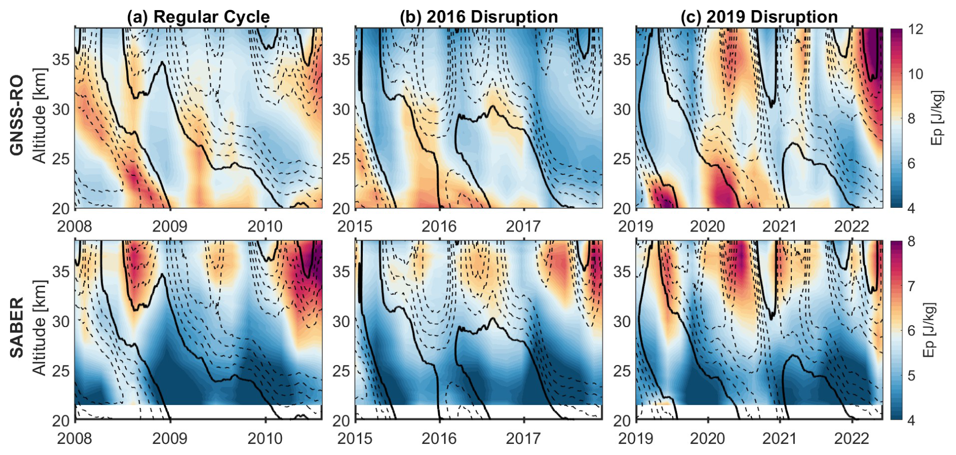
Figure A1Time-Height cross-section of a color map of GW Ep from GNSS-RO (top row) and SABER (bottom row) overlaid by the zonal winds at the QBO region shown in contour lines, with solid lines represent zero-wind line and dashed lines represent the westward winds with a spacing of 5 m s−1 during one regular cycle (a) the 2016 disruption (b) and the 2019 disruption (c).
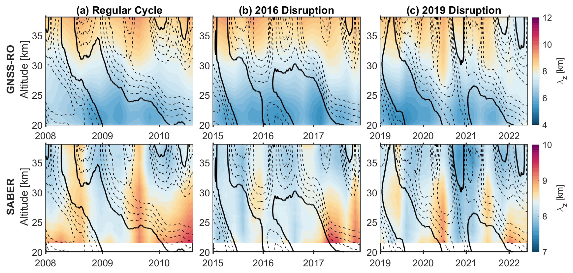
The repository of GNSS-RO data in the AWS Registry of Open Data can be found at http://registry.opendata.aws/gnss-ro-opendata/ (last access: 1 November 2025). Documentation of the repository, source code for the API, and tutorial demonstrations are published under a digital object identifier (Leroy and McVey, 2023). The database API is published through PyPI; see http://pypi.org/project/awsgnssroutils/ (last access: 1 November 2025). The SABER/TIMED data used in this work can be obtained from https://saber.gats-inc.com/ (last access: 1 November 2025). DYAMONDv2 data can be accessed via the NCCS Dataportal – Datashare (https://portal.nccs.nasa.gov/datashare/G5NR/DYAMONDv2/, last access: 1 November 2025).
The conceptualization of the study, software, and validation of the results were done by MA, CW, and NH. Formal analysis was done by MA and CW. Investigation, visualization, and writing the original draft are done by MA. Data curation, funding acquisition, and project administration was done by CW. Methodology and supervision were done by CW and NH. All authors contributed to the interpretation of the results and the final text.
The contact author has declared that none of the authors has any competing interests.
Publisher’s note: Copernicus Publications remains neutral with regard to jurisdictional claims made in the text, published maps, institutional affiliations, or any other geographical representation in this paper. While Copernicus Publications makes every effort to include appropriate place names, the final responsibility lies with the authors. Views expressed in the text are those of the authors and do not necessarily reflect the views of the publisher.
This study was supported by the UK Natural Environment Research Council (NERC) under grant numbers NE/W003201/1 supporting M. Almowafy, C. Wright and N. Hindley, and NE/V01837X/1 supporting C. Wright. N. Hindley was also supported by a NERC Independent Research Fellowship NE/X017842/1, and C. Wright was also supported a Royal Society University Research Fellowship URF/R/221023. M. Almowafy and C. Wright were additionally supported by Royal Society grant no. RF/ERE/221011. DYAMOND data management was provided by the German Climate Computing Center (DKRZ) and supported through the projects ESiWACE and ESiWACE2. The projects ESiWACE and ESiWACE2 have received funding from the European Union’s Horizon 2020 research and innovation programme under grant agreements No 675191 and 823988. This work used resources of the Deutsches Klimarechenzentrum (DKRZ) granted by its Scientific Steering Committee (WLA) under project IDs bk1040 and bb1153. This research was supported by the International Space Science Institute (ISSI) in Bern, through ISSI International Team project #567. The ChatGPT LLM was used for minor refinements of textual style at the individual-sentence level, but all scientific results were obtained using non-AI methods. We thank the reviewer for their suggestions, which have added valuable insights to this paper. The lead author would like to dedicate this work to her brother, Abdulrahman Almowafy, who passed away in May 2024.
This research has been supported by the Natural Environment Research Council, National Centre for Atmospheric Science (grant no. NE/W003201/1), the Natural Environment Research Council, National Centre for Atmospheric Science (grant no. NE/V01837X/1), the Natural Environment Research Council, National Centre for Atmospheric Science (grant no. NE/X017842/1), and the Royal Society (grant nos. RF/ERE/221011 and URF/R/221023).
This paper was edited by Wen Yi and reviewed by two anonymous referees.
Alexander, M. J., Geller, M., McLandress, C., Polavarapu, S., Preusse, P., Sassi, F., Sato, K., Eckermann, S., Ern, M., Hertzog, A., Kawatani, Y., Pulido, M., Shaw, T. A., Sigmond, M., Vincent, R., and Watanabe, S.: Recent developments in gravity-wave effects in climate models and the global distribution of gravity-wave momentum flux from observations and models, Quarterly Journal of the Royal Meteorological Society, 136, 1103–1124, 2010. a
Alexander, M. J.: Interpretations of observed climatological patterns in stratospheric gravity wave variance, Journal of Geophysical Research: Atmospheres, 103, 8627–8640, https://doi.org/10.1029/97JD03325, 1998. a, b, c
Alexander, M. J. and Holton, J. R.: On the spectrum of vertically propagating gravity waves generated by a transient heat source, Atmos. Chem. Phys., 4, 923–932, https://doi.org/10.5194/acp-4-923-2004, 2004. a
Alexander, P., de la Torre, A., and Llamedo, P.: Interpretation of gravity wave signatures in GPS radio occultations, J. Geophys. Res., 113, D16117, https://doi.org/10.1029/2007JD009390, 2008. a, b, c
Anstey, J. A., Banyard, T. P., Butchart, N., Coy, L., Newman, P. A., Osprey, S., and Wright, C. J.: Prospect of Increased Disruption to the QBO in a Changing Climate, Geophysical Research Letters, 48, e2021GL093058, https://doi.org/10.1029/2021GL093058, 2022. a, b, c
Anthes, R. A., Ector, D. R., Hunt, D. C., Kuo, Y.-H., Rocken, C., Schreiner, W. S., Sokolovskiy, S., Syndergaard, S., Wee, T.-K., Zeng, Z., Bernhardt, P., Dymond, K., Chen, Y., Liu, H., Manning, K. W., Randel, W., Trenberth, K. E., Cucurull-Ector, L., Healy, S., and Yen, N.: The COSMIC/FORMOSAT-3 Mission: Early results, Bulletin of the American Meteorological Society, 89, 313–333, https://doi.org/10.1175/BAMS-89-3-313, 2008. a
Baldwin, M. P., Gray, L. J., Dunkerton, T. J., Hamilton, K., Haynes, P. H., Randel, W. J., Holton, J. R., Alexander, M. J., Hirota, I., Horinouchi, T., Jones, D. B. A., Kinnersley, J. S., Marquardt, C., Sato, K., and Takahashi, M.: The quasi-biennial oscillation, Reviews of Geophysics, 39, 179–229, https://doi.org/10.1029/1999RG000073, 2001. a
Brown, S. B., Jensen, M., Jensen, S., Hansen, G., Zollinger, L., Esplin, R., and Miller, J. B.: Sounding of the atmosphere using broadband emission radiometry (SABER): Sensor design, performance, and lessons learned, Proc. SPIE 6297, Infrared Spaceborne Remote Sensing XIV, 62970U, https://doi.org/10.1117/12.684137, 2006. a
de la Torre, A. and Alexander, P.: Gravity waves above Andes detected from GPS radio occultation temperature profiles: Mountain forcing?, Geophysical Research Letters, 32, https://doi.org/10.1029/2005GL022959, 2005. a, b, c
De la Torre, A., Schmidt, T., and Wickert, J.: A global analysis of wave potential energy in the lower stratosphere derived from 5 years of GPS radio occultation data with CHAMP, Geophysical Research Letters, 33, https://doi.org/10.1029/2006GL027696, 2006. a
Dunkerton, T. J.: The role of gravity waves in the quasi-biennial oscillation, Journal of Geophysical Research: Atmospheres, 102, 26053–26076, https://doi.org/10.1029/96JD02999, 1997. a
Ern, M., Preusse, P., Gille, J. C., Hepplewhite, C. L., Mlynczak, M. G., Russell III, J. M., and Riese, M.: Implications for atmospheric dynamics derived from global observations of gravity wave momentum flux in stratosphere and mesosphere, Journal of Geophysical Research: Atmospheres, 116, https://doi.org/10.1029/2011JD015821, 2011. a
Ern, M., Ploeger, F., Preusse, P., Gille, J. C., Gray, L. J., Kalisch, S., Mlynczak, M. G., Russell III, J. M., and Riese, M.: Interaction of gravity waves with the QBO: A satellite perspective, Journal of Geophysical Research: Atmospheres, 119, 2329–2355, https://doi.org/10.1002/2013JD020731, 2014. a, b, c, d, e, f
Ern, M., Trinh, Q. T., Preusse, P., Gille, J. C., Mlynczak, M. G., Russell III, J. M., and Riese, M.: GRACILE: a comprehensive climatology of atmospheric gravity wave parameters based on satellite limb soundings, Earth Syst. Sci. Data, 10, 857–892, https://doi.org/10.5194/essd-10-857-2018, 2018. a, b
Faber, A., Llamedo, P., Schmidt, T., de la Torre, A., and Wickert, J.: On the determination of gravity wave momentum flux from GPS radio occultation data, Atmos. Meas. Tech., 6, 3169–3180, https://doi.org/10.5194/amt-6-3169-2013, 2013. a, b
Fan, Z. Q., Sheng, Z., Shi, H. Q., Yi, X., Jiang, Y., and Zhu, E. Z.: Comparative Assessment of COSMIC Radio Occultation Data and TIMED/SABER Satellite Data over China, Journal of Applied Meteorology and Climatology, 54, 1931–1943, https://doi.org/10.1175/JAMC-D-14-0151.1, 2015. a
Gelaro, R., Putman, W. M., Pawson, S., Draper, C., Molod, A., Norris, P. M., Ott, L., Privé, N., Reale, O., Achuthavarier, D., Bosilovich, M., Buchard, V., Chao, W., Coy, L., Cullather, R., da Silva, A., Darmenov, A., Errico, R. M., Fuentes, M., Kim, M.-J., Koster, R., McCarty, W., Nattala, J., Partyka, G., Schubert, S., Vernieres, G., Vikhliaev, Y., and Wargan, K.: Evaluation of the 7-km GEOS-5 Nature Run, Technical Memorandum (TM), https://ntrs.nasa.gov/citations/20150011486 (last access: 3 November 2025), 2015. a
Heale, C., Walterscheid, R., and Snively, J.: Localization effects on the dissipation of gravity wave packets in the upper mesosphere and lower thermosphere, Journal of Geophysical Research: Atmospheres, 123, 8915–8935, 2018. a
Hersbach, H., Bell, B., Berrisford, P., Dahlgren, P., Horányi, A., Muñoz-Sabater, J., Nicolas, J., Radu, R., Schepers, D., Simmons, A., and Soci, C.: The ERA5 Global Reanalysis: achieving a detailed record of the climate and weather for the past 70 years., EGU General Assembly 2020, Online, 4–8 May 2020, EGU2020-10375, https://doi.org/10.5194/egusphere-egu2020-10375, 2020. a, b
Hindley, N. P., Wright, C. J., Smith, N. D., and Mitchell, N. J.: The southern stratospheric gravity wave hot spot: individual waves and their momentum fluxes measured by COSMIC GPS-RO, Atmos. Chem. Phys., 15, 7797–7818, https://doi.org/10.5194/acp-15-7797-2015, 2015. a, b, c
Hindley, N. P., Wright, C. J., Hoffmann, L., Moffat-Griffin, T., and Mitchell, N. J.: An 18-Year Climatology of Directional Stratospheric Gravity Wave Momentum Flux From 3-D Satellite Observations, Geophysical Research Letters, 47, e2020GL089557, https://doi.org/10.1029/2020GL089557, 2019a. a
Hindley, N. P., Wright, C. J., Smith, N. D., Hoffmann, L., Holt, L. A., Alexander, M. J., Moffat-Griffin, T., and Mitchell, N. J.: Gravity waves in the winter stratosphere over the Southern Ocean: high-resolution satellite observations and 3-D spectral analysis, Atmos. Chem. Phys., 19, 15377–15414, https://doi.org/10.5194/acp-19-15377-2019, 2019b. a
Hindley, N. P., Mitchell, N. J., Cobbett, N., Smith, A. K., Fritts, D. C., Janches, D., Wright, C. J., and Moffat-Griffin, T.: Radar observations of winds, waves and tides in the mesosphere and lower thermosphere over South Georgia island (54° S, 36° W) and comparison with WACCM simulations, Atmos. Chem. Phys., 22, 9435–9459, https://doi.org/10.5194/acp-22-9435-2022, 2022. a, b, c, d
Ho, S.-p., Zhou, X., Shao, X., Chen, Y., Jing, X., and Miller, W.: Using the Commercial GNSS RO Spire Data in the Neutral Atmosphere for Climate and Weather Prediction Studies, Remote Sens., 15, 4836, https://doi.org/10.3390/rs15194836, 2023. a
Hoffmann, L., Günther, G., Li, D., Stein, O., Wu, X., Griessbach, S., Heng, Y., Konopka, P., Müller, R., Vogel, B., and Wright, J. S.: From ERA-Interim to ERA5: the considerable impact of ECMWF's next-generation reanalysis on Lagrangian transport simulations, Atmos. Chem. Phys., 19, 3097–3124, https://doi.org/10.5194/acp-19-3097-2019, 2019. a
Holt, L. A., Alexander, M. J., Coy, L., Molod, A., Putman, W., and Pawson, S.: Tropical Waves and the Quasi-Biennial Oscillation in a 7-km Global Climate Simulation, Journal of the Atmospheric Sciences, 73, 3771–3783, https://doi.org/10.1175/JAS-D-15-0350.1, 2016. a, b
Holt, L. A., Alexander, M. J., Coy, L., Liu, C., Molod, A., Putman, W., and Pawson, S.: An evaluation of gravity waves and gravity wave sources in the Southern Hemisphere in a 7 km global climate simulation, Quarterly Journal of the Royal Meteorological Society, 143, 2481–2495, https://doi.org/10.1002/qj.3101, 2017. a, b
Holton, J. R., Alexander, M. J., and Boehm, M. T.: Evidence for short vertical wavelength Kelvin waves in the Department of Energy-Atmospheric Radiation Measurement Nauru99 radiosonde data, Journal of Geophysical Research: Atmospheres, 106, 20125–20129, https://doi.org/10.1029/2001JD900108, 2001. a
John, S. R. and Kumar, K. K.: TIMED/SABER observations of global gravity wave climatology and their interannual variability from stratosphere to mesosphere lower thermosphere, Climate Dynamics, 39, 1489–1505, 2012. a
Kim, Y.-H., Voelker, G. S., Bölöni, G., Zängl, G., and Achatz, U.: Crucial role of obliquely propagating gravity waves in the quasi-biennial oscillation dynamics, Atmos. Chem. Phys., 24, 3297–3308, https://doi.org/10.5194/acp-24-3297-2024, 2024. a
Krebsbach, M. and Preusse, P.: Spectral analysis of gravity wave activity in SABER temperature data, Geophysical Research Letters, 34, https://doi.org/10.1029/2006GL028040, 2007. a
Kursinski, E. R., Hajj, G. A., Schofield, J. T., Linfield, R. P., and Hardy, K. R.: Observing Earth's atmosphere with radio occultation measurements using the Global Positioning System, Journal of Geophysical Research: Atmospheres, 102, 23429–23465, https://doi.org/10.1029/97JD01569, 1997. a, b, c, d
Lear, E., Wright, C., Hindley, N., Polichtchouk, I., and Hoffmann, L.: Comparing Gravity Waves in a Kilometer-Scale Run of the IFS to AIRS Satellite Observations and ERA5, Journal of Geophysical Research: Atmospheres, 129, e2023JD040097, https://doi.org/10.1029/2023JD040097, 2024. a, b, c
Leroy, S.: GNSS Radio Occultation Data in the AWS Open Data Registry, https://registry.opendata.aws/gnss-radio-occultation/ (last access: 19 September 2024), 2022. a
Leroy, S. and McVey, A.: GNSS radio occultation data in the AWS cloud: Utilities and examples, Zenodo, https://doi.org/10.5281/zenodo.7799039, 2023. a
Leroy, S. S., McVey, A. E., Leidner, S. M., Zhang, H., and Gleisner, H.: GNSS Radio Occultation Data in the AWS Cloud, Earth and Space Science, 11, e2023EA003021, https://doi.org/10.1029/2023EA003021, 2023. a, b, c, d, e
Li, H., Zhang, J., Sheng, B., Fan, Y., Ji, X., and Li, Q.: The gravity wave activity during two recent qbo disruptions revealed by us high-resolution radiosonde data, Remote Sensing, 15, 472, https://doi.org/10.3390/rs15020472, 2023. a, b
Liu, X., Yue, J., Xu, J., Garcia, R. R., Russell III, J. M., Mlynczak, M., Wu, D. L., and Nakamura, T.: Variations of global gravity waves derived from 14 years of SABER temperature observations, Journal of Geophysical Research: Atmospheres, 122, 6231–6249, 2017. a, b
Luo, J., Hou, J., and Xu, X.: Variations in stratospheric gravity waves derived from temperature observations of multi-gnss radio occultation missions, Remote Sensing, 13, 4835, https://doi.org/10.3390/rs13234835, 2021. a, b
Mertens, C., Russell, J., Mlynczak, M., She, C., Schmidlin, F., Goldberg, R., Lopezpuertas, M., Wintersteiner, P., Picard, R., and Winick, J.: Kinetic temperature and carbon dioxide from broadband infrared limb emission measurements taken from the TIMED/SABER instrument, Advances in Space Research, 43, 15–27, https://doi.org/10.1016/j.asr.2008.04.017, 2009. a
Mlynczak, M. G.: Energetics of the mesosphere and lower thermosphere and the SABER experiment, Adv. Space Res., 20, 1177–1183, 1997. a, b
Namboothiri, S., Jiang, J., Kishore, P., Igarashi, K., Ao, C., and Romans, L.: CHAMP observations of global gravity wave fields in the troposphere and stratosphere, Journal of Geophysical Research: Atmospheres, 113, D07102, https://doi.org/10.1029/2007JD008912, 2008. a
Nath, D., Chen, W., and Guharay, A.: Climatology of stratospheric gravity waves and their interaction with zonal mean wind over the tropics using GPS RO and ground-based measurements in the two phases of QBO, Theoretical and Applied Climatology, 170, https://doi.org/10.1007/s00704-014-1146-7, 2014. a, b, c, d, e
Osprey, S. M., Butchart, N., Knight, J. R., Scaife, A. A., Hamilton, K., Anstey, J. A., Schenzinger, V., and Zhang, C.: An unexpected disruption of the atmospheric quasi-biennial oscillation, Science, 353, 1424–1427, https://doi.org/10.1126/science.aah4156, 2016. a, b, c
Poli, P. and Joiner, J.: Assimilation experiments of one-dimensional analyses with GPS/MET refractivity, in: First CHAMP Mission Results for Gravity, Magnetic and Atmospheric Studies, 515–520, Springer, New York, https://doi.org/10.1007/978-3-540-38366-6_70, 2003. a, b
Preusse, P., Eckermann, S. D., and Offermann, D.: Comparison of global distributions of zonal-mean gravity wave variance inferred from different satellite instruments, Geophysical Research Letters, 27, 3877–3880, 2000. a
Preusse, P., Eckermann, S. D., Ern, M., Oberheide, J., Picard, R. H., Roble, R. G., Riese, M., Russell III, J. M., and Mlynczak, M. G.: Global ray tracing simulations of the SABER gravity wave climatology, Journal of Geophysical Research: Atmospheres, 114, ADA522332, https://doi.org/10.1029/2008JD011214, 2009. a, b, c
Putman, W., da Silva, A. M., Ott, L. E., and Darmenov, A.: Model Configuration for the 7-km GEOS-5 Nature Run, Ganymed Release (Non-hydrostatic 7 km Global Mesoscale Simulation), Tech. rep., GMAO Office Note No. 5 (Version 1.0), 18 pp., https://gmao.gsfc.nasa.gov/pubs/docs/Putman727.pdf (last access: 10 January 2025), 2014. a
Remsberg, E. E.: Assessment of the quality of the version 1.07 temperature-versus-pressure profiles of the middle atmosphere from TIMED/SABER, J. Geophys. Res., 113, D17101, https://doi.org/10.1029/2008JD010013, 2008. a, b, c
Rocken, C., Van Hove, T., and Ware, R.: Near real-time GPS sensing of atmospheric water vapor, Geophysical Research Letters, 24, 3221–3224, https://doi.org/10.1029/97GL03312, 1997. a
Russell, J. M., Mlynczak, M. G., Gordley, L. L., Tansock, J. J., and Esplin, R. W.: Overview of the SABER experiment and preliminary calibration results, Proc. SPIE 3756, Optical Spectroscopic Techniques and Instrumentation for Atmospheric and Space Research III, https://doi.org/10.1117/12.366382, 1999. a
Schmidt, T., de la Torre, A., and Wickert, J.: Global gravity wave activity in the tropopause region from CHAMP radio occultation data, Geophysical Research Letters, 35, https://doi.org/10.1029/2008GL034986, 2008. a
Schmidt, T., Alexander, P., and de la Torre, A.: Stratospheric gravity wave momentum flux from radio occultations, Journal of Geophysical Research: Atmospheres, 121, 4443–4467, https://doi.org/10.1002/2015JD024135, 2016. a, b
Shuai, J., Zhang, S., Huang, C., Yi, F., Huang, K., Gan, Q., and Gong, Y.: Climatology of global gravity wave activity and dissipation revealed by SABER/TIMED temperature observations, Science China Technological Sciences, 57, 998–1009, 2014. a
Stephan, C. C., Duras, J., Harris, L., Klocke, D., Putman, W. M., Taylor, M., Wedi, N. P., Žagar, N., and Ziemen, F.: Atmospheric Energy Spectra in Global Kilometre-Scale Models, Tellus A: Dynamic Meteorology and Oceanography, https://doi.org/10.16993/tellusa.26, 2022. a, b
Stockwell, R. G., Mansinha, L., and Lowe, R.: Localization of the complex spectrum: the S transform, IEEE Transactions on Signal Processing, 44, 998–1001, 1996. a, b
Trinh, Q. T., Kalisch, S., Preusse, P., Chun, H.-Y., Eckermann, S. D., Ern, M., and Riese, M.: A comprehensive observational filter for satellite infrared limb sounding of gravity waves, Atmos. Meas. Tech., 8, 1491–1517, https://doi.org/10.5194/amt-8-1491-2015, 2015. a, b, c, d, e
Tsuda, T., Nishida, M., Rocken, C., and Ware, R. H.: A Global Morphology of Gravity Wave Activity in the Stratosphere Revealed by the GPS Occultation Data (GPS/MET), Journal of Geophysical Research: Atmospheres, 105, 7257–7273, https://doi.org/10.1029/1999JD901005, 2000. a, b
Tsuda, T., Venkat Ratnam, M., Alexander, S. P., Kozu, T., and Takayabu, Y.: Temporal and spatial distributions of atmospheric wave energy in the equatorial stratosphere revealed by GPS radio occultation temperature data obtained with the CHAMP satellite during 2001–2006, Earth, Planets and Space, 61, 525–533, 2009. a, b, c, d
Tsuda, T., Lin, X., Hayashi, H., and Noersomadi: Analysis of vertical wave number spectrum of atmospheric gravity waves in the stratosphere using COSMIC GPS radio occultation data, Atmos. Meas. Tech., 4, 1627–1636, https://doi.org/10.5194/amt-4-1627-2011, 2011. a, b
Vincent, R. A. and Alexander, M. J.: Balloon-Borne Observations of Short Vertical Wavelength Gravity Waves and Interaction With QBO Winds, Journal of Geophysical Research: Atmospheres, 125, e2020JD032779, https://doi.org/10.1029/2020JD032779, 2020. a
Wang, L. and Alexander, M. J.: Global estimates of gravity wave parameters from GPS radio occultation temperature data, Journal of Geophysical Research: Atmospheres, 115, https://doi.org/10.1029/2010JD013860, 2010. a, b, c, d, e
Wickert, J., Beyerle, G., Hajj, G. A., Schwieger, V., and Reigber, C.: GPS radio occultation with CHAMP: Atmospheric profiling utilizing the space-based single difference technique, Geophysical Research Letters, 29, 28-1–28-4, https://doi.org/10.1029/2001GL013982, 2002. a, b
Wright, C. and Gille, J.: Detecting overlapping gravity waves using the S-Transform, Geophysical Research Letters, 40, 1850–1855, 2013. a
Wright, C. J. and Hindley, N. P.: How well do stratospheric reanalyses reproduce high-resolution satellite temperature measurements?, Atmos. Chem. Phys., 18, 13703–13731, https://doi.org/10.5194/acp-18-13703-2018, 2018. a, b, c, d, e, f, g, h
Wright, C. J., Osprey, S. M., Barnett, J. J., Gray, L. J., and Gille, J. C.: High Resolution Dynamics Limb Sounder measurements of gravity wave activity in the 2006 Arctic stratosphere, Journal of Geophysical Research: Atmospheres, 115, https://doi.org/10.1029/2009JD011858, 2010. a
Wright, C. J., Rivas, M. B., and Gille, J. C.: Intercomparisons of HIRDLS, COSMIC and SABER for the detection of stratospheric gravity waves, Atmos. Meas. Tech., 4, 1581–1591, https://doi.org/10.5194/amt-4-1581-2011, 2011. a, b, c, d, e, f
Wright, C. J., Hindley, N. P., Moss, A. C., and Mitchell, N. J.: Multi-instrument gravity-wave measurements over Tierra del Fuego and the Drake Passage – Part 1: Potential energies and vertical wavelengths from AIRS, COSMIC, HIRDLS, MLS-Aura, SAAMER, SABER and radiosondes, Atmos. Meas. Tech., 9, 877–908, https://doi.org/10.5194/amt-9-877-2016, 2016. a, b, c, d, e, f, g, h, i
Wright, C. J., Hindley, N. P., Hoffmann, L., Alexander, M. J., and Mitchell, N. J.: Exploring gravity wave characteristics in 3-D using a novel S-transform technique: AIRS/Aqua measurements over the Southern Andes and Drake Passage, Atmos. Chem. Phys., 17, 8553–8575, https://doi.org/10.5194/acp-17-8553-2017, 2017. a
Wright, C. J., Ungermann, J., Preusse, P., and Polichtchouk, I.: Using sub-limb observations to measure gravity waves excited by convection, npj Microgravity, 9, 14, https://doi.org/10.1038/s41526-023-00259-2, 2023. a
Wu, D. L., Preusse, P., Eckermann, S. D., Jiang, J. H., de la Torre Juarez, M., Coy, L., and Wang, D. Y.: Remote sounding of atmospheric gravity waves with satellite limb and nadir techniques, Advances in Space Research, 37, 2269–2277, https://doi.org/10.1016/j.asr.2005.07.031, 2006. a, b, c
Yee, J.-H., Talaat, E. R., Christensen, A. B., Killeen, T. L., Russell, J. M., and Woods, T. N.: TIMED instruments, Johns Hopkins APL Tech. Dig., 24, 156–164, 2003. a
Yiğit, E. and Medvedev, A. S.: Role of gravity waves in vertical coupling during sudden stratospheric warmings, Geoscience Letters, 3, 27, https://doi.org/10.1186/s40562-016-0056-1, 2016. a
Zhang, Y., Xiong, J., Liu, L., and Wan, W.: A global morphology of gravity wave activity in the stratosphere revealed by the 8-year SABER/TIMED data, Journal of Geophysical Research: Atmospheres, 117, https://doi.org/10.1029/2012JD017676, 2012. a
- Abstract
- Introduction
- Data
- Methods
- SABER and GNSS-RO Observation Results
- Model Sampled Data
- Adjusting Observations
- Summary and Discussion
- Conclusions
- Appendix A: Supplementary Figures
- Data availability
- Author contributions
- Competing interests
- Disclaimer
- Acknowledgements
- Financial support
- Review statement
- References