Toolbox for accurate estimation and validation of Positive Matrix Factorization solutions in Particulate Matter source apportionment

Positive matrix factorization (PMF) is the most commonly used approach for particulate matter source apportionment; however, the implementation steps of the model require considerable user experience. Most studies apply PMF according to the recommendations of the Environmental Protection Agency and the European Commission, while relatively few studies focus on further developing the PMF methodology. This study aims to develop a systematic method that reduces some subjective aspects when performing a PMF study, providing recommendations and tools for its application and validation. A total of 13 targeted tests were conducted to address key sources of subjectivity in PMF, categorized into three critical aspects: preparation of the input matrix, selecting the number of sources, and validation of the PMF solution. The results of the first step highlighted that using a single source tracer reduces the tracer's dispersion into other sources, leading to more accurate results. The second stage tests suggested that the selection of a source tracer should be based on low uncertainty and specific temporal evolution, in order to facilitate the determination of a new source without compromising the PMF solution. Finally, the validation step was set up as an advanced comparison of the PMF-derived source profiles with those in the literature, including SPECIEUROPE database, using the ratio of chemicals and distance metrics. All outcomes of this study are compiled into a Python package providing essential tools to support the work from PMF implementation to solution validation, leading to less subjective solutions and more rigorous and reliable source apportionment.

1 Introduction

Receptor models are widely used for atmospheric particulate matter source apportionment (PM SA), assigning the PM sources using measurements at a receptor site. Positive matrix factorization (PMF), developed by Paatero and Tappert (1994), has been the most popular receptor model for PM SA (Hopke, 2016). PMF is frequently performed using EPA PMF software developed by the US – Environmental Protection Agency. A Fundamentals and User Guide was launched along with the software, providing a general guide for implementing PMF for all environment domains (Norris et al., 2014). Focusing especially on the air pollution SA, the Forum for Air Quality Modeling (FAIRMODE), which is chaired by the European Commission Joint Research Centre, reported a harmonized receptor model protocol that recommended different aspects of PMF implementation, including input matrix, uncertainty calculation, and the number of sources (Belis et al., 2014). Apart from these reports, most studies essentially use PMF, with few studies considering the improvement of the methodology (Hopke et al., 2020). There remains a lack of recommendations regarding aspects that require user decisions, as some of these have not yet been systematically tested to provide “educated guesses”.

However, some efforts to improve the PMF methodology have been established over the years, including (1) developing tools to estimate the uncertainties of PMF results and apply PMF for big data (Brown et al., 2015; Hopke et al., 2023), (2) developing tools to compare chemical profiles (Belis et al., 2015), (3) adding new tracers representing the organic sources (Borlaza et al., 2021b; Glojek et al., 2024; Hu et al., 2010; Lu et al., 2018; Mardoñez et al., 2023; Samaké et al., 2019b; Wang et al., 2012), (4) standardizing the PMF implementation methodology (Chen et al., 2022; Weber et al., 2019), (5) Combining multiple sites to reduce the rotational ambiguity of the PMF (Hernández-Pellón and Fernández-Olmo, 2019; Pandolfi et al., 2020; Pietrodangelo et al., 2024; Dai et al., 2020), (6) incorporating meteorological data to the PMF (Dai et al., 2021) and, (7) improving result visualizations (PyPMF – https://pypmf.readthedocs.io, last access: 20 April 2025; Weber et al., 2019).

Indeed, PMF analysis involves several steps that require subjective choices from the user. Since prior information is not required to perform a PMF study, the results obtained with the model strongly depend on these users' decisions. One example of this is the input data set chosen, which orientates the determination of the sources, as reported by Amato et al. (2024), demonstrating that the lack of tracers of a source obviously prevents its identification. It raises questions on the basic data set for the mandatory input for meaningful work. Further, the calculation method of input data uncertainties could influence the PMF solution stability, including the scaled residual and bootstrap results (Waked et al., 2014). As another example, Belis et al. (2015) indicated that the number of sources obtained can broadly vary according to the expertise of the group performing a PMF study, as demonstrated from the comparison of PM SA results generated by 38 research groups on the same dataset. Finally, constraints that can be applied to initial results to obtain the final solution rely on user experience, and their application criteria as well as the error of the solution (Bootstrap, DISP) are rarely documented in the literature (Hopke, 2016). In the same way, comparison of the chemical profiles obtained in the studies is rarely benchmarked towards previous results.

The present study describes some further developments and tests in an attempt to improve the robustness of the PMF methodology by proposing pathways for narrowing the subjective choices of the users by testing some of the limits of the methodology, particularly when it comes to the choice of variables and the number of sources. We also propose some toolkits for quicker preparation, evaluation, and benchmarking of the results during the trial and error phases of the implementation of a PMF study. These different steps are presented for several studies conducted with the EPA PMF 5.0 software using databases of PM₁₀ sample series analyzed in recent years within various programs conducted in France.

2 Methodology

2.1 General organization of the approach

Performing a PMF study is a complex process, including a large number of steps with trial and error testing and feedback loops, where many implementation steps require subjectivity in the user's choices, as presented in Fig. S1 in the Supplement. These choices include, among others, input matrix preparation, selection of the number of factors, and result validation criteria. In this study, we performed tests on these different steps, with (1) tests on the input matrix, evaluating the variations induced in the PMF solution by including or excluding specific tracers, (2) tests performed on the selection of the number of sources, providing recommendations for selecting the tracers of sources, (3) PMF output evaluation by comparing PMF-derived chemical profile with that reported in the literature. The details of each test and the data used for each of them are presented in Table 1 and Sect. 2.1.1, 2.1.2, and 2.1.3, respectively. This work is based on the series of PM₁₀ samples collected in several projects, also detailed in Table 1.

Table 1 Tests performed, as described in Sect. 2.1.1, 2.1.2, and 2.1.3.

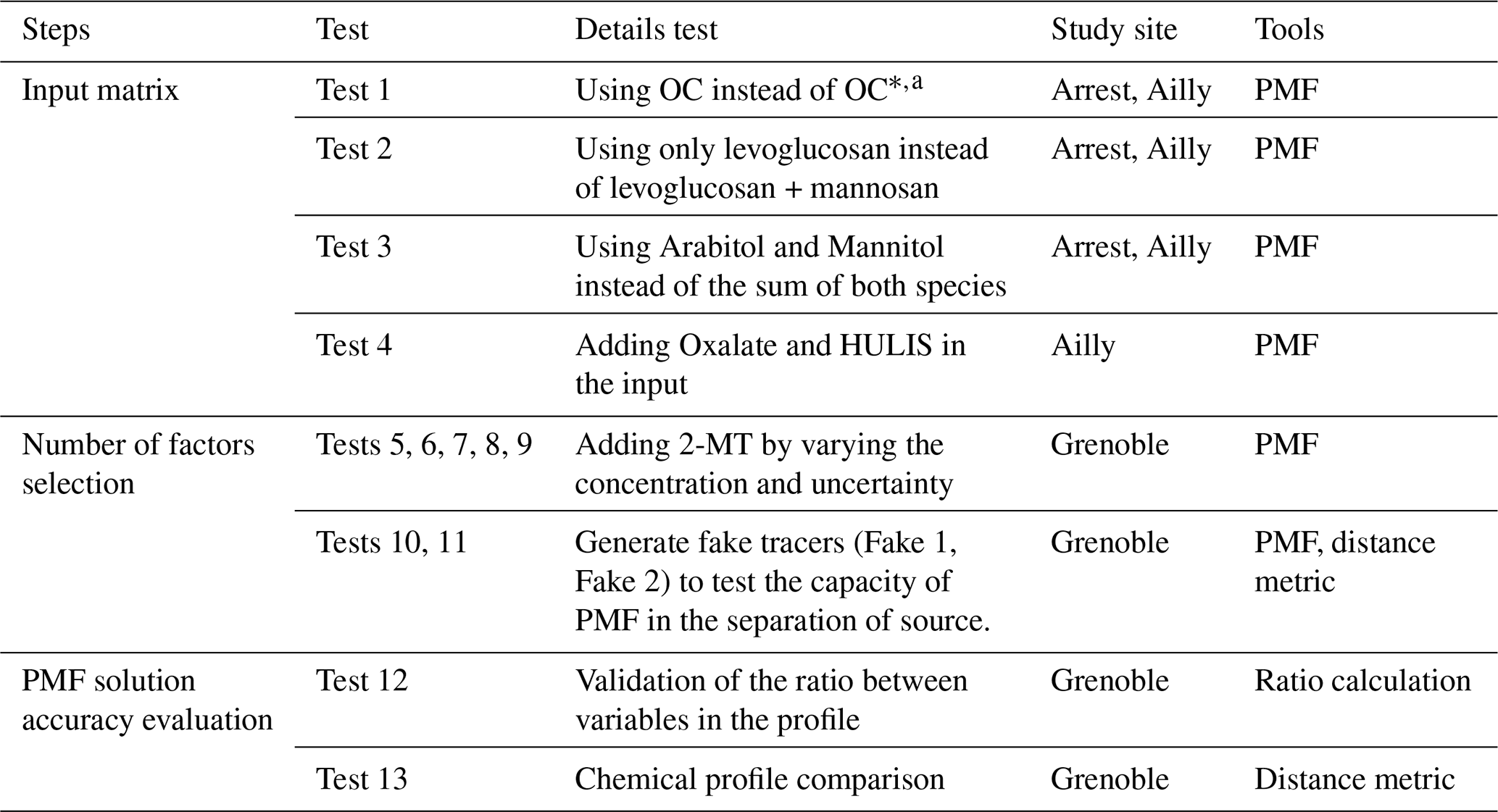
^a OC^∗ is calculated by Eq. (S1).

2.1.1 Tests on input matrix

Four tests were performed to evaluate the PMF solution sensitivity by modifying the input matrix (Table 1). These tests were performed on a large dataset with about 220 samples analyzed for an extensive array of chemical components (see Sect. 2.2.1). Tests 1 to 3 test the sensitivity of some changes in the input data for some commonly used compounds (OC, levoglucosan, polyols). Conversely, test 4 incorporates chemical species that are rarely added to PMF (oxalate, HUmic LIke Substances – HULIS) to both explore their impact on the results and investigate their sources in PM₁₀.

Many PMF studies make use of OC^∗ instead of OC – as an input variable to avoid double-counting part of the total OC mass (Eq. S1) (Borlaza et al., 2021b; Dominutti et al., 2024; Srivastava et al., 2018). To do so, authors generally retrieve from OC the carbon contents included in the used input organic variables. Such a prior data handling is notably included as a recommendation in the European guidance for PM SA (Belis et al., 2014). Test 1 compares the results of using this approach or not. In test 2, a single tracer of biomass Burning (BB) (levoglucosan) is considered instead of two (levoglucosan and mannosan), to evaluate the stability of the PMF solution to such changes. In test 3, a similar approach is adopted, comparing PMF results when using a “Polyols” input (sum of concentrations of arabitol and mannitol), instead of each chemical species separately. It is well known that these sugar alcohols are associated with biogenic activities from fungi (Samaké et al., 2019a; Yttri et al., 2007), and can then be considered as tracers for primary biogenic aerosols. In test 4, the PMF input incorporates two organic compounds that have a crucial mass contribution to OC, (i.e., HULIS and Oxalate) and are also mainly known as secondary products of primary emissions from different sources. This test aims to provide information on the stability of the factors obtained with more straightforward data sets, and also investigate the sources of these secondary organic components in the atmosphere. The inputs of Test 1 to 4 and the PMF base run are presented in Table S1.

2.1.2 Tests on the number of factors and the number of chemical tracers

The number of factors chosen for an optimal solution is commonly selected based on the statistical parameters of initial PMF runs. The basic parameter considered in this approach is $Q_{\mathrm{true}}/Q_{\mathrm{expect}}$, which is the ratio between the goodness of fit of the solution and the expected one. The Q_expect is calculated using the number of samples, factors, and number of chemicals included in the input matrix (Belis et al., 2014). The optimal number of sources is selected when this ratio approaches 1 (Belis et al., 2014). Other criteria are then further evaluated, which are: the geochemical likelihood of the solutions, the uncertainty of the solution (bootstrap, displacement), and the statistical parameters of the solution (residual, R²). However, the number of factors observed in the literature is rarely larger than 10 to 12 for well-documented PMF studies. Tests 5 to 11 investigate whether such a number of factors present an inherent limit of the PMF process or if it is related to the structure and content of the database. We tried to investigate the intrinsic capability of the PMF methodology to delineate further sources when proper tracers are included in the input data set.

On the basis of a 11 factors' PMF solution obtained with a yearly time series of observations in Grenoble (France) (Borlaza et al., 2021b), we conducted tests 5 to 9 by adding a tracer of biogenic oxidation products (2-methyltetrols, (2MT), coming from the oxidation of isoprene (Carlton et al., 2009; Edney et al., 2005)) on top of the 3-MBTCA (tracer of the Secondary Organic Aerosol (SOA) formed from the alpha-pinene oxidation (Claeys et al., 2007; Kourtchev et al., 2008)), aiming to separate these two SOA sources. The time series of their respective concentrations differ, but the initial 11 factors of PMF work could not properly separate the two factors. The concentrations and uncertainty of 2-MT were changed conditionally (resulting in different $S/N$) to assess how these parameters influence the source separation. This was further investigated with tests 10 and 11, where a synthetic series of tracers was generated using the criteria defined in tests 5–9 to validate their efficiency and delineate additional sources. The inputs of each test and the PMF solutions are presented in Table S2.

2.1.3 Tools to evaluate the PMF result

To evaluate PMF outputs, each obtained factor is questioned as possibly being representative of a given emission source and/or secondary formation process based on its chemical profile and timeseries, generally according to the operator's knowledge and experience. There are indeed few guidelines and tools that allow the benchmarking of these choices, which are rarely fully backed up in the presentation of PMF works. In order to provide a more objective way of testing the reliability of the results from a PMF study, we implemented two tools to evaluate the chemical profiles obtained. The first one is based on a compilation of diagnostic ratios available in the literature concerning some common chemical species used in PMF studies in order to test automatically if the results of PMF are in agreement with these ratios. The detailed expected range of the ratio, the reference, as well as the type of source according to ratio value are presented in Table S3 in the Supplement. The Python code for this tool is proposed in a Python package, called PMF_toolkits (https://github.com/DinhNgocThuyVy/PMF_toolkits, last access: 24 April 2025), and an example of the application is proposed in Test 12.

A second tool is proposed to automatically compare the full chemical profiles obtained in the PMF output with banks of known chemical profiles. The database is extracted from the European Commission sources profile repository SPECIEUROPE (Table S4) (Pernigotti et al., 2016). It has been augmented with some recent sources reported in the literature that are not yet available in the repository, including all the ones generated from past studies in France from our group (IGE database) that are currently being transferred (Table S5).

2.2 Study site and chemical analysis

2.2.1 Study sites

PM₁₀ series of samples from three different French sites were used for these 15 tests: Arrest, Ailly, and Grenoble (Table 1). The sampling date, frequency, and number of samples are shown in Table 2. The chemical analyses of these samples are briefly described in Sect. 2.2.2. They are detailed, along with their corresponding initial PMF outputs (used as the basis for the present paper), in Zhang et al. (2024) for the Arrest and Ailly sites and in Borlaza et al. (2021b) for the Grenoble sites.

Table 2 Sites description.

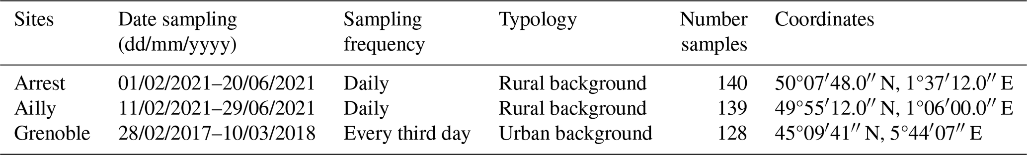
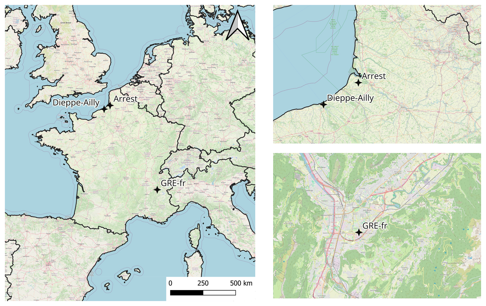
Figure 1 Location of Ailly, Arrest and Grenoble © OpenStreetMap contributors 2025. Distributed under the Open Data Commons Open Database License (ODbL) v1.0.

Arrest and Ailly are located in coastal rural sites in the north of France (Fig. 1b), which are 50 km apart. Arrest covers an area of 11.15 km² and has a population of 855, representing a density of 77 inhabitants km⁻². The agglomeration of Ailly, with a population of 46 223, occupies an area of 5.7 km². Eleven sources were identified in the PM₁₀ for each site: Aged sea salt, biomass burning (BB), MSA-rich, heavy oil combustion (HFO), industrial, mineral dust, nitrate-rich, primary biogenic, primary traffic, sea salt, secondary biogenic.

Grenoble is an urban background site located in an Alpine valley southeast of France (Fig. 1c), sprawling over 18.13 km² with 154 018 inhabitants in 2023 with a density of 800 inhabitants km⁻². The initial PMF work in Grenoble identified 10 sources of PM₁₀, including aged sea salt, BB, industrial, mineral dust, nitrate-rich, primary biogenic, primary traffic, sea/road salt, secondary biogenic, and sulfate-rich.

2.2.2 Chemical analysis

The daily PM₁₀ sampling was performed using high-volume samplers (Digitel DA80, 30 m³ h⁻¹) using 150 mm-diameter pure quartz fibre filter (Tissu-quartz PALL QAT-UP 2500 diameter 150 mm). A standard protocol was applied for cleaning, unloading, packing, and storing filters to avoid contamination. Field blank filters were collected (about 8 %–12 % of the number of samples) to estimate the detection limit and control the filter contaminations. This protocol is presented in Weber et al. (2019) and Borlaza et al. (2021b).

The PM₁₀ filter samples were extracted to perform chemical analysis for quantifying different PM components, including the main components by mass and many tracers of sources, including carbonaceous fractions (OC, EC), major ionic species (Cl⁻, NO${}_{\mathrm{3}}^{-}$, SO${}_{\mathrm{4}}^{\mathrm{2}-}$, Na⁺, NH${}_{\mathrm{4}}^{+}$, K⁺, Mg²⁺, Ca²⁺), methanesulfonic acid (MSA), Oxalate, HULIS, 3-methyl-1,2,3-butanetricarboxylic acid (3-MBTCA), anhydrous sugar and saccharides (levoglucosan, mannosan, arabitol, mannitol) and metals (Al, As, Ba, Cd, Co, Cu, Fe, Mn, Ni, Pb, Rb, Se, Sr, Ti, V, Zn). Details of chemical analysis are presented in Borlaza et al. (2021b).

In brief, the elemental carbon (EC) and organic carbon (OC) were analyzed using a Sunset Lab analyzer (Birch and Cary, 1996) based on the EUSAAR2 thermo-optical protocol.

The filters were punched using 11.34 cm² punches, soaked in 10 mL of ultra-pure water, and filtered after 20 min of agitation using a 0.25 µm porosity filter. These water extracts were used for the following analysis. The major ionic components, MSA, and Oxalate, were analyzed using an ICS3000 dual-channel chromatograph (Thermo-Fisher) with a CS12 column for cations analysis and an AS11HC column for anions analysis. The anhydrous-sugar and saccharides analysis was carried out on the aqueous phase by high-performance liquid chromatography (HPLC) with Pulsed Amperometric Detection (PAD) (model Dionex DX500 + ED40). HPLC-PAD was performed using a Thermo-Fisher ICS 5000+ HPLC equipped Metrosep Carb column and precolumn in isocratic mode. 3-MBTCA was analyzed using the HPLC coupled mass spectroscopy (HPLC-MS) with negative mode electrospray ionization.

HULIS measurement was conducted according to the protocol reported by Baduel et al. (2010). Briefly, the analysis was performed on the water-soluble fraction of filter samples. The neutral components, hydrophobic bases, inorganic anions, mono- and di-acids are removed by passing through a weak anion exchange resin. After extraction, HULIS quantification is performed using a TOC analyzer (Shimazdu).

Finally, the filters were punched into a 38 mm diameter, mineralized and used to conduct the analysis of major and trace elements. The analysis was performed using inductively coupled plasma mass spectroscopy (ICP-MS) (ELAN 6100 DRC II PerkinElmer or NEXION PerkinElmer) (Alleman et al., 2010).

2.3 PMF

The PMF methodology is used to perform Tests 1 to 11, using EPA PMF 5.0 software. The PMF input variables of all tests are shown in Table S1 for Test 1 to Test 4 and Table S2 for Test 5 to Test 11. The PMF theory, briefly described in Sect. 2.3.1 and 2.3.2, points out the crucial parameters in PMF execution. In Tests 5 to 11, the inputs are conditionally generated, as presented in Sect. 2.3.3.

2.3.1 PMF formula

PMF algorithm based on observed concentration data (matrix X) to identify the contribution of the factors (matrix G) and factors profiles (matrix F) as described in the equations below:

$$\begin{array}{}\text{(1)}& {\displaystyle }{\mathbf{X}}_{ij}=\sum _{k=\mathrm{1}}^p{\mathbf{G}}_{ik}\ast {\mathbf{F}}_{kj}+E_{ij}\text{(2)}& {\displaystyle }{\mathbf{G}}_{ik}\ge \mathrm{0},{\mathbf{F}}_{ik}\ge \mathrm{0}\end{array}$$

Where X is a (i×j) matrix of j chemical species in measured period i (generally daily sampling) into p factors with a matrix (i×k) representing the source contribution (G) and a matrix (k×j) representing the factor composition (F). E is the residual for each species. All the factor matrices G and F elements are constrained to be non-negative.

The solutions are selected by finding F and G to obtain the minimum value of the quality of fit parameter (Q), which is calculated by:

$$\begin{array}{}\text{(3)}& {\displaystyle }Q=\sum _{i=\mathrm{1}}^n\sum _{j=\mathrm{1}}^m{E}_{ij}^{\mathrm{2}}/{\mathit{\sigma }}_{ij}^{\mathrm{2}}\text{(4)}& {\displaystyle }\left\{G,F\right\}=\mathrm{argmin}Q\end{array}$$

Where ${\mathit{\sigma }}_{ij}^{\mathrm{2}}$ is the known uncertainties for each data value xij (arranged in uncertainty matrix of input data). The higher the uncertainty, the lower the ratio $E_{ij}^{\mathrm{2}}/{\mathit{\sigma }}_{ij}^{\mathrm{2}}$, consequently lesser influence on Q calculation. Thus, chemical species with high uncertainty have a diminished effect on the PMF model.

2.3.2 Signal-to-noise ratio

The signal-to-noise ratio ($S/N$) represents the relationship between the concentration and uncertainty of a species (Eqs. 5, 6, 7). A species with $S/N$ < 0.2 means concentrations are almost equal to uncertainties, and it has to be removed from the model to avoid unreliable results. Conversely, a $S/N$ value > 2 (where concentration > 3 times uncertainty) is considered satisfactory enough to consider the corresponding variable as a “Strong” one. Between 0.2 and 2, the specie will be categorized as “Weak”, and the uncertainties is set to 3 times the original one (Belis et al., 2014).

$$\begin{array}{}\text{(5)}& {\displaystyle }{\left({\displaystyle \frac{S}{N}}\right)}_j={\displaystyle \frac{\mathrm{1}}{n}}\sum _{i=\mathrm{1}}^n{d}_{ij}\text{(6)}& {\displaystyle }{d}_{ij}=\left({\displaystyle \frac{x_{ij}-s_{ij}}{s_{ij}}}\right),\mathrm{if}{x}_{ij}>s_{ij}\text{(7)}& {\displaystyle }{d}_{ij}=\mathrm{0},\mathrm{if}{x}_{ij}\le s_{ij}\end{array}$$

with x_ij is concentration and s_ij is the uncertainty of measured period i in chemicals j.

Therefore, $S/N$ is an indicator of the influence of a chemical specie on the Q calculation. This indicator is used in Tests 5 to 9 to elucidate the importance of uncertainty in the separation of a factor in PMF.

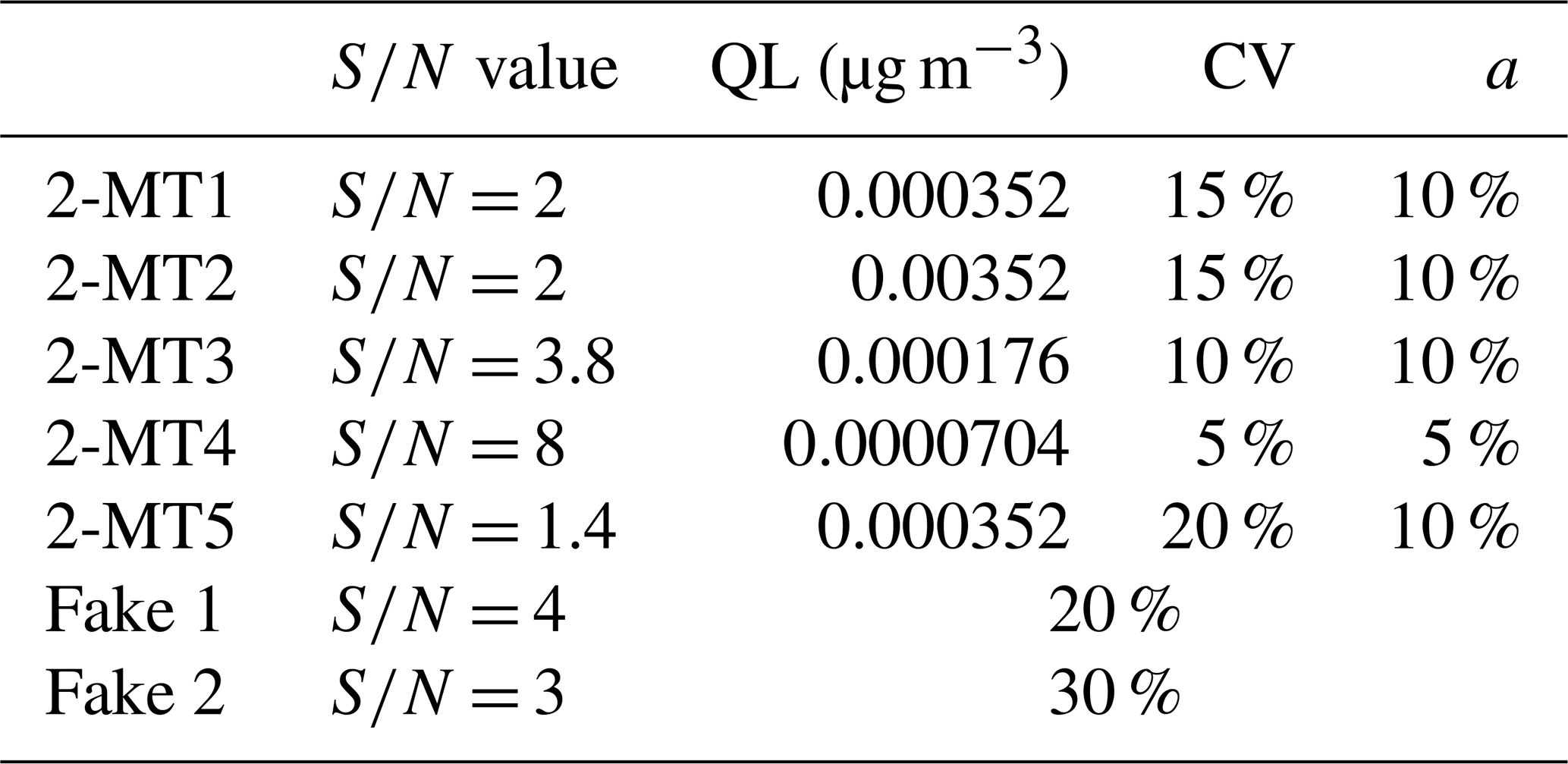
2.3.3 The generation of variable characteristics of 2-MT for sensitivity tests

The uncertainty is calculated using the formula of Gianini et al. (2012), presented in Table S6. The uncertainties of the test component (2-MT) for the sensitivity tests in Sect. 2.1.2 are generated by varying the limit of quantification (QL), coefficient variation (CV), and additional coefficient (a) (Table 3), resulting in the $S/N$ value ranging from 1 to 8. The concentration and time series of the component are also changed to evaluate the effects on the PMF result, as presented in Fig. S2.

Table 3 $S/N$ value corresponding to parameters used for uncertainty calculation of 2-MT and Fake 1, Fake 2.

2.4 Distance metrics

The comparisons between the PMF-derived chemical profiles and the SPECIATE + IGE database are performed with the two distance metrics Pearson Distance (PD) and Similarity Identity Distance (SID). These distances are reported by Belis et al. (2015), and are calculated by Eqs.(8) and (9). The PD is sensitive to the main composition of PM, while SID represents the similarity of all common components of the paired comparison of chemical profile and, therefore, also includes the influence of minor chemical species by mass. The chemical profiles are declared similar if 0 < SID < 1 and PD < 0.4.

$$\begin{array}{}\text{(8)}& \mathrm{PD}=\mathrm{1}-R^{\mathrm{2}}\end{array}$$

where R² is the Pearson coefficient of the relative mass to PM of all components between 2 chemical profiles

$$\begin{array}{}\text{(9)}& \mathrm{SID}={\displaystyle \frac{\sqrt{\mathrm{2}}}{m}}{\sum }_{j=\mathrm{1}}^m{\displaystyle \frac{\left|x_j-y_j\right|}{x_j+y_y}}\end{array}$$

Where m is the number of chemical species common to both profiles, with x and y the relative mass of these m to the PM in the two respective chemical profiles.

3 Result and discussion

3.1 Tests on the PMF inputs

3.1.1 Tests on the sensitivity of the PMF of changes in commonly used chemical species

Tests 1, 2, and 3 evaluate the efficiency and usefulness of some choices for the variables in the PMF inputs for the PMF work in the two sites, Ailly and Arrest. The comparison of source contribution to PM between the base run solutions and Tests 1, 2, 3 (Fig. 2) shows a good stability PMF over all tests and both sites, with a consistency for the number of factors (remaining at 11 sources) and a maximum difference in source contribution to PM among tests being limited to 1 % for Arrest and 3 % for Ailly.

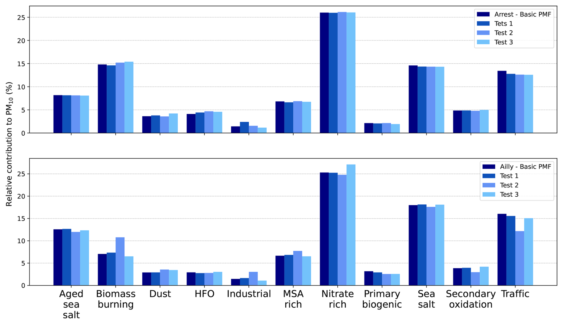
Figure 2 PM₁₀ source contributions of base run PMF and Test 1, 2, 3 in Arrest (Upper) and Ailly (Lower).

Test 1 shows negligible variation in all factors compared to the base run PMF solution in both sites when using OC or OC^∗. The difference between the two concentrations is relatively low, only 6 % and 3 % of the OC mass for Arrest and Ailly, respectively. The stable total reconstructed PM concentrations, the unchanging number of sources, and the stable contributions of each factor suggest that it may not be necessary to use OC^∗, at least in cases when the mass difference between OC and OC^∗ is below 6 %. Similar results were obtained for another study in an Alpine Valley site (Glojek et al., 2024), where the difference between the two concentrations is 10 %.

Test 2, comparing the results using a single BB tracer (levoglucosan) vs. using both tracers, levoglucosan and mannosan (in the base run), also indicates a relatively low change in PM contribution. The highest changes are observed in the contribution of BB (increases from 7 % to 10 %). A closer examination of the chemical profiles shows that with a single tracer, there is less dispersion of chemical species of interest in the other sources (in this case, levoglucosan, OC, EC). Especially for the traffic source, where the presence of levoglucosan is not really justified based on geochemical knowledge (Borlaza et al., 2021a; Weber et al., 2019), a reduction of 5 % of levoglucosan is observed (compared to the base PMF run). This reduction results in a lower contribution of OC and EC in the traffic profile, eventually decreasing the contribution of traffic to PM₁₀. The bootstrap values from this test indicated a reduced traffic swap with the other sources compared to the base run PMF (Table S7). In addition, test 2 conducted a more homogenous PM contribution of BB between Arrest and Ailly (15 % vs. 11 %), located 50 km apart. Consequently, test 2 strongly suggests the benefits of using levoglucosan instead of levoglucosan and mannosan.

This strongly suggests that using a single, robust tracer is preferable. While PMF can group correlated variables, including multiple highly collinear tracers in the input data can introduce rotational ambiguity that risks biasing the model's outcome. This can lead to the misattribution of these tracers to other factors, thereby altering their chemical profiles and contributions.

Test 3 considers using the sum of concentrations of arabitol and mannitol (base run) instead of the two chemical species separately as proper tracers of primary biogenic emission associated with fungal spores (Bauer et al., 2002; Rogge et al., 2007; Samaké et al., 2019b; Yttri et al., 2011). Similar to test 2, test 3 reveals only minimal change in the factor associated with these tracers, with a decrease of 0.5 % in the contribution of the primary biogenic source to PM. This change also results from more dispersion of arabitol and mannitol to the other sources, compared to the use of their sum (as “Polyols”). Although the contribution demonstrates minor variation, this result again suggests the advantage of using a single tracer. As mentioned above, it seems again that using two separate tracers can lead to their larger distribution in some other sources, resulting in a decrease in the contribution of their source and some degree of mixing.

3.1.2 Tests on adding new chemical species

Test 4 incorporated HULIS and Oxalate simultaneously into PMF to evaluate the impacts of these changes in the input data and investigate the possibility of determining their fate in the atmosphere. Indeed, these two compounds are known as secondary organic products, and ubiquitous. They are generally the main components identified in the OM. Developing a better knowledge of the sources of their main precursor, along with the evaluation of the ability of the PMF method to deliver such information, is therefore of interest for AQ plans. Test 4 indicates that the optimal number of sources when adding these chemicals remains stable at 11 sources. The main statistical parameters (BS values and reconstruction of PM) are not impacted (Table S7), and the chemical profiles remain unchanged except for these two chemical species, which seems in itself a good appraisal of the base run PMF solution stability. Hence, these results potentially provide some novel insights into the relation to the primary sources for these secondary organic fractions, which are rarely discussed.

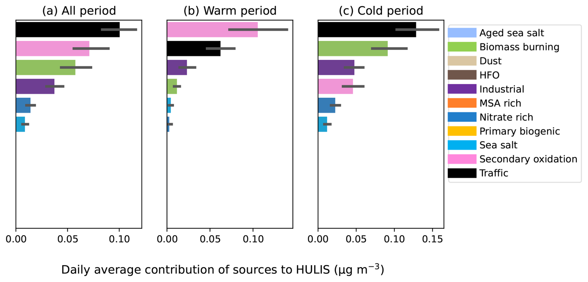
Figure 3 Daily average sources contribution to HULIS (µg m⁻³) in (a) the study period, (b) the warm period (April, May, June), and cold period (February, Mars) in Ailly. The bars represent the mean, and the error bars represent the 90 % confidence interval of the mean.

HULIS are consistently associated with traffic, secondary biogenic oxidation, BB, and industrial activities during the whole observation period (Fig. 3a), all sources that are mainly involved in the emission of OM. HULIS are also presented in the nitrate-rich and sea salt sources, with a lower contribution. This partially aligns with a PM source apportionment that incorporated HULIS in a study in Beijing and reported that the most important source of HULIS is coal/ BB and traffic (Dominutti et al., 2024; Li et al., 2019; Srivastava et al., 2018). In addition, current research has suggested that HULIS are predominantly linked to combustion processes during the winter period, either by direct emissions or by the secondary formation in the processing of these emissions, and are supposed to be mainly anthropogenic (Baduel et al., 2010; Graber and Rudich, 2006; Zheng et al., 2013). Our results align with the concepts reported in these studies, which demonstrated that the primary sources in the cold period are traffic and BB (Fig. 3c). On the other hand, in summer, the main sources are the production of secondary biogenic organic aerosol and traffic (Fig. 3b). During summer, polymerization or oligomerization processes activated by higher temperature, light intensity, high volatile organic compounds (VOCs) and O₃ or OH radical concentration can produce photochemical reactions leading to HULIS formations (Hoffer et al., 2006; Wu et al., 2018). In addition, Zheng et al. (2013) suggested that the VOCs generated by vehicles are critical precursors of HULIS through heterogeneous reactions.

Figure 4 The relative contribution of the source to Oxalate (a) in Ailly and (b) in Arrest.

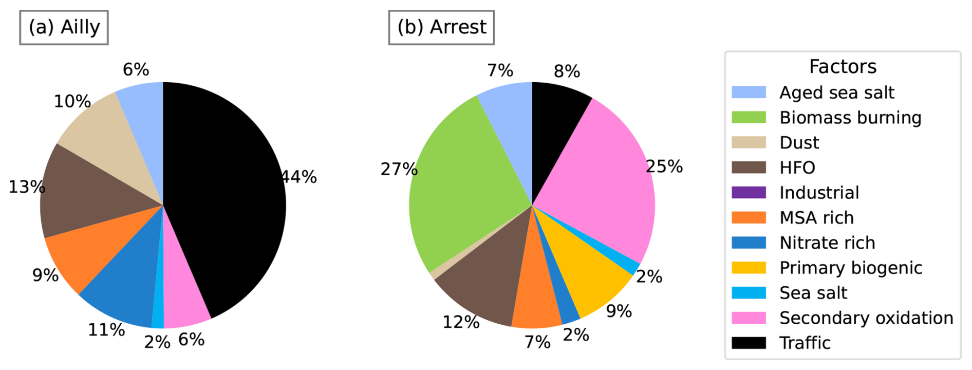
In Ailly, oxalate is mainly associated with traffic (44 %), HFO (13 %), nitrate-rich (11 %), and dust (10 %) (Fig. 4a). In contrast, in Arrest, oxalate is predominantly associated with BB (27 %) and secondary biogenic organic aerosol traced by 3-MBTCA (25 %). This discrepancy can be attributed to the sampling locations, as the site in Ailly is closer to roads and the parking of a cultural landmark and also immediately next to the seashore. Therefore, the contributions of oxalate are primarily related to traffic and marine sources (including intense shipping emissions in the English Channel). In contrast, Arrest's sampling site is entirely separated from the main roads and surrounded by large natural areas (marsh area in the Baie de Somme). Therefore, the origins of oxalate depicted in our PMF results could be plausible. Indeed, these sources are in line with several studies that discussed the main origins of oxalate, like Zhou et al. (2015), who indicated that oxalate is related to secondary processes of BB emission aging, or Kawamura and Bikkina (2016) who suggested that oxalate may be derived from traffic emissions, associated with oxidation of compounds derived from gasoline combustion engines and residual oil combustion. The same authors also found a linear relationship between oxalate and methane sulfonic acid (MSA), explaining it by the fact that aged sea salt includes unsaturated fatty acids that can form oxalate by further photochemical oxidation processes.

Finally, this test is interesting because it confirms that introducing secondary species that we know come from several sources does not lead to new independent sources despite their significant contribution to the total carbon mass. Further, this does not disturb the previous sources from the base run but leads to the repartition of these species into reasonable sources, opening the door to understanding their formation process in more detail.

However, on the contrary, the introductions of some other organic species (not reported in this specific work) were not so successful, and we failed to obtain reasonable solutions or new factors with the introduction in the input PMF data of specific species like MSA (a known tracer of oxidation products from marine VOC emissions (Li et al., 1993)), cellulose (a known tracer of plant debris (Brighty et al., 2022)), or 2-methyltetrols (2-MT) (a known tracer of oxidation products from isoprene (Edney et al., 2005)), among others. Some of these trials are reported in Glojek et al. (2024). Obviously, the capacity of PMF to separate a source does not depend solely on the introduction of a proper tracer, even with a specific time series (Glojek et al., 2024), but also on other aspects, some of which are tentatively investigated in the next Sect. 3.2.

3.2 The ultimate determination of source number

The following series of tests (5 to 9) are performed with the base case of the Grenoble times series (Borlaza et al., 2021b) (Table 1). They investigate the impact of some changes in the characteristics of the 2-MT time series of concentrations in order to evaluate the conditions necessary to obtain a specific factor associated with secondary oxidation from the isoprene emission. This essentially includes changes in concentrations and uncertainties ($S/N$ values), as shown in Table 4. In addition, Tests 10 and 11 try to evaluate the capability of PMF to generate more than 11 or 12 factors when appropriate tracers are introduced in the input data. This is tested with the generation of “fake components” (Fake 1 and Fake 2), with characteristics (time series, concentrations, $S/N$) guided by the previous tests 5 to 9 for defining “a proper tracer”.

Table 4 The description of input and output statistical parameters of Test 5 to Test 11. x represents non-identify.

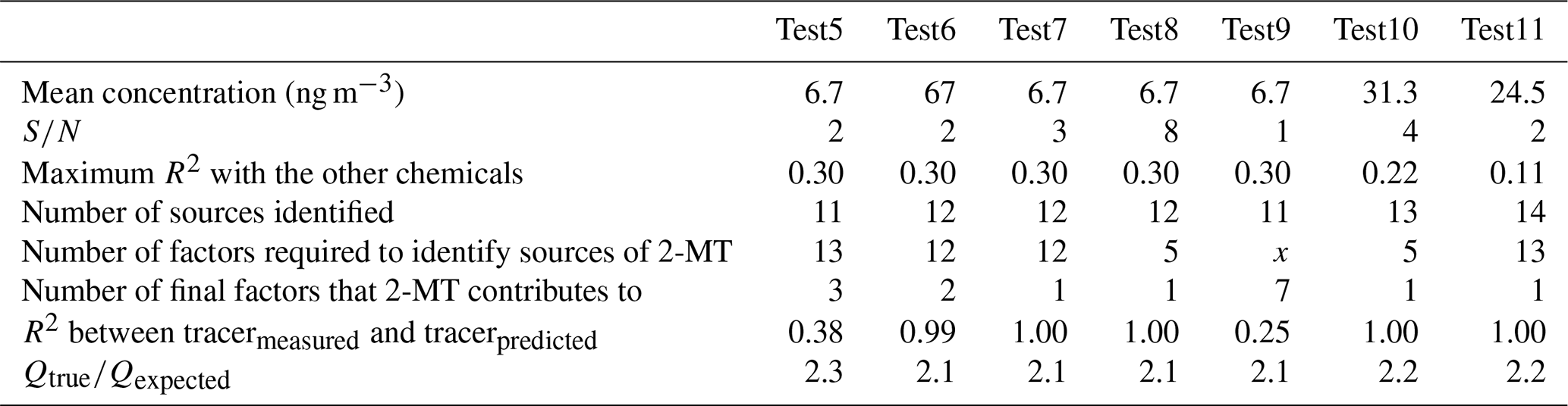
It should first be noted that the time series of 2-MT (based on real measurements), Fake 1 and Fake 2 are quite different from that of all other chemical species from the input matrix (Fig. S3), and particularly all of the biogenic tracers. The best correlation is obtained between 2-MT and MSA, with an R² of 0.30, for 128 samples, preventing collinearity. Table 4 includes some of the results from these tests, including the optimal number of sources identified, the number of sources including a substantial fraction of the 2-MT (for test 5 to test 9), Fake 1 and Fake 2 (test 10, 11, respectively), and the performance of reproduction of their concentrations by the PMF. It should be noted that all 20 runs performed for each test converged, and constraints “Pull up maximally” for the source tracer were applied to improve the base run results (Table S8).

For Tests 5 and 9, with the actual measured concentrations of 2-MT and $S/N$ values < 2, the PMF does not allow the identification of a specific source for 2-MT, with a number of sources identical to the base run (11 sources). 2-MT contributes to 3 sources in Test 5 (higher $S/N$) and 7 in Test 9 (lower $S/N$) (Fig. S4). Although the principal attribution is to primary biogenic in both tests, the reconstruction of the species is better in test 5, resulting in an R² between observed and predicted concentration of 0.38 vs. 0.25 for test 5 and test 9, respectively. Even though the performances are better for the higher $S/N$ and the tracer has no strong collinearity with other factors, the results in Tests 5 and 9 do not provide a separate factor.

The PMF solution is improved in test 6, with the combination of $S/N$ = 2 and a higher concentration (10 times higher than the measured concentration of 2-MT), allowing the identification of a new source comprising most of the 2-MT (98 %). Tests 7 and 8, which have the measured concentrations but higher $S/N$ values, also facilitated the separation of 2-MT into an additional 12th source, comprising 100 % of the tracer in both tests (Fig. S4). Due to very high seasonality, the mass fraction associated with this source is only meaningful during a short period, reaching about 2 %–3 % only in July–August. Interestingly, we observed that the $S/N$ also affects the ability to identify the source: in the PMF process, the source of 2-MT appears when five sources are selected with $S/N$ = 8, while with $S/N$ ≤ 3 in (Tests 6 and 7), it is identified later when 12 sources are selected. Finally, it is worth noting that the $Q_{\mathrm{true}}/Q_{\mathrm{expected}}$ ratio is relatively stable and not a good indicator for the choice of the proper number of sources at this stage of the resolution of the PMF.

All these tests tend to indicate that the $S/N$ value is the most important criterion that allows the separation of a specific factor in a complex PMF with about 8–10 factors, with a value of $S/N$ above 2–3 being a threshold above which separation can be effective. It seems that the higher the value, the easier the separation of the specific factor. High concentration may play a role for source identification, but it is not essential in source contribution (contribution of 2-MT source to PM is similar for test 6 and test 7). However, this is also conditional on a time series of the concentration of a specific tracer that presents low collinearity with other tracers, a value of R² < 0.3 for about 100 or more samples being advisable. Consequently, the result recommends key criteria for tracer selection with (1) the $S/N$ ≥ 3 and (2) remarkable temporal evolution, where the R² between the tracer and other chemical species in the input matrix is below 0.3.

With Tests 11 and 12, we tried to verify if these criteria are valid for increasing the number of factors that are possible to delineate for a PMF study in this range of 10–15 sources, using reconstructed (fake) time series. The Fake 1 and Fake 2 components are generated with criteria as in Table 4, and then successively incorporated into the input database of Test 7. Table 4 indicates that the PMF enables the identification of 13 and 14 sources for Test 10 and Test 11, respectively, with excellent reconstructions of the fake tracers (R² = 1).

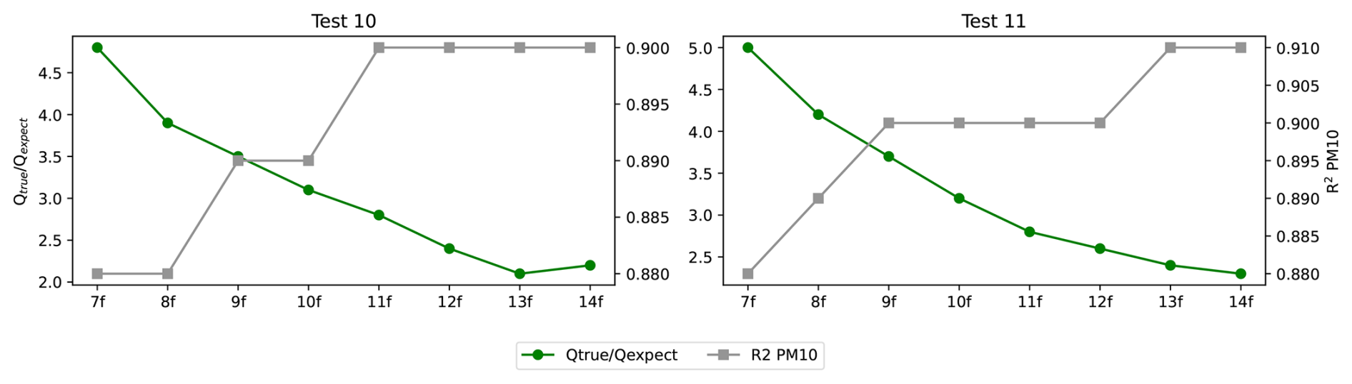
Figure 5 The variation of R² between observed PM₁₀ and predicted PM₁₀ and ratio $Q_{\mathrm{true}}/Q_{\mathrm{robust}}$ over the number of factors of Test 10 (left) and Test 11 (right).

The extensive descriptions of the PMF solution, including the reconstructed level of PMF (R² between predicted and observed concentration), bootstrap values, and displacement (DISP) in Test 10 and Test 11 (Table S9 and S10), demonstrate the robustness of solutions. The narrow band of DISP values of 2-MT, Fake 1 and Fake 2 in their source (Table S10), highlights the low rotation variation of these tracers. The variation of the ratio $Q_{\mathrm{true}}/Q_{\mathrm{expected}}$ and R² of PM${}_{\mathrm{10}}^{\mathrm{obs}}$ and PM${}_{\mathrm{10}}^{\mathrm{predicted}}$ (Fig. 5) shows that the solutions reached the lowest $Q_{\mathrm{true}}/Q_{\mathrm{expected}}$ and highest R² at 13 factors for test 10 and 14 for test 11. Notably, the $Q_{\mathrm{true}}/Q_{\mathrm{expected}}$ close to 2 is observed as the most appropriate, indicating the identical ratio for all tests (see Table 4).

In addition, the chemical profile of the sources from Test 5 to 11 and the base run PMF 11 factors solution is compared using PD and SID, indicating that the chemical profiles are all within an excellent homogeneity range (Fig. S5). This last point emphasized that incorporating 2-MT, Fake 1, and Fake 2 does not affect the initial solution. Finally, all these tests clearly indicate that valid solutions with at least up to 14 different sources are possible with the PMF, providing that the input includes tracers with low collinearity and $S/N$ above three.

3.3 Chemical profile comparison

3.3.1 Validation of the ratio between chemicals/tracers in the profile

While the ratio of specific chemical species has long been used in many studies (particularly concerning trace elements) for the tentative evaluation of the sources of PM components, these diagnostic ratios are very rarely checked in PMF studies for the validation of the PMF solutions presented. We tried to implement an automatic tool for easily performing such validations, using an extended table of plausible ranges of ratios obtained from the literature for many common sources obtained in PMF studies.

This step is preliminary to the evaluation of the appropriateness of a PMF solution. A solution with a chemical profile that significantly exceeds the accepted range should be further investigated to confirm the geochemical meaningfulness of sources for the specific sampling site. The tools to compare the specific ratio of chemicals in the profile of PMF-derived sources and literature have been developed (detailed in Sect. S1, Supplement) and can be accessed at https://github.com/DinhNgocThuyVy/PMF_toolkits.

Table 5 Comparison of the ratio between chemicals in the source profile of Grenoble and the literature.

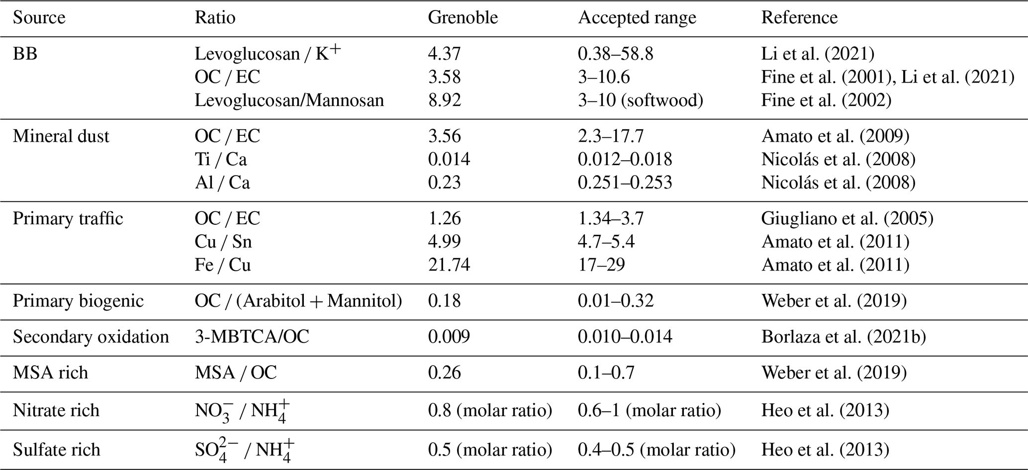
Table 5 presents the results of some specific ratios for the sources obtained in the 11-factor base run solution of the study in Grenoble used in the previous sections. It indicates that the PMF solution is globally well aligned with the diagnostic ratios reported in the literature. Some deviation can be seen for the mineral dust (Al $/$ Ca) and primary traffic factor (OC $/$ EC), which is supposed to be negligible since the discrepancy is relatively low (the ratio in Grenoble is lower than 8 % compared to that reported in the references).

3.3.2 Chemical profile comparison – biomass burning source

Following the previous test about diagnostic ratio, the results obtained for the sources from a PMF study could be benchmarked for their full chemical profiles against those obtained in the literature. We developed another tool for the automatic comparison with chemical profiles from 2 databases (SPECIEUROPE and SPECIEUROPE + IGE). The comparison aims to point out if the profiles obtained in a PMF work are similar to those reported in the literature, but also to provide insight into naming as properly as possible a factor identified by the PMF (which is also a critical step, particularly for an air quality regulation perspective). The comparison is performed using the Pearson distance (PD) and Similarity Identity Distance (SID) (Belis et al., 2015). The criteria for selecting similar profiles in the database are as follows: (1) PD < 1, (2) 0 < SID < 1, (3) number of chemicals used for comparison (n) > 50 % of the chemical species in the PMF-derived source. Ultimately, the most similar chemical profile (compared to the profile to be evaluated) is selected by sorting the lowest PD ∩ the lowest SID ∩ the highest n.

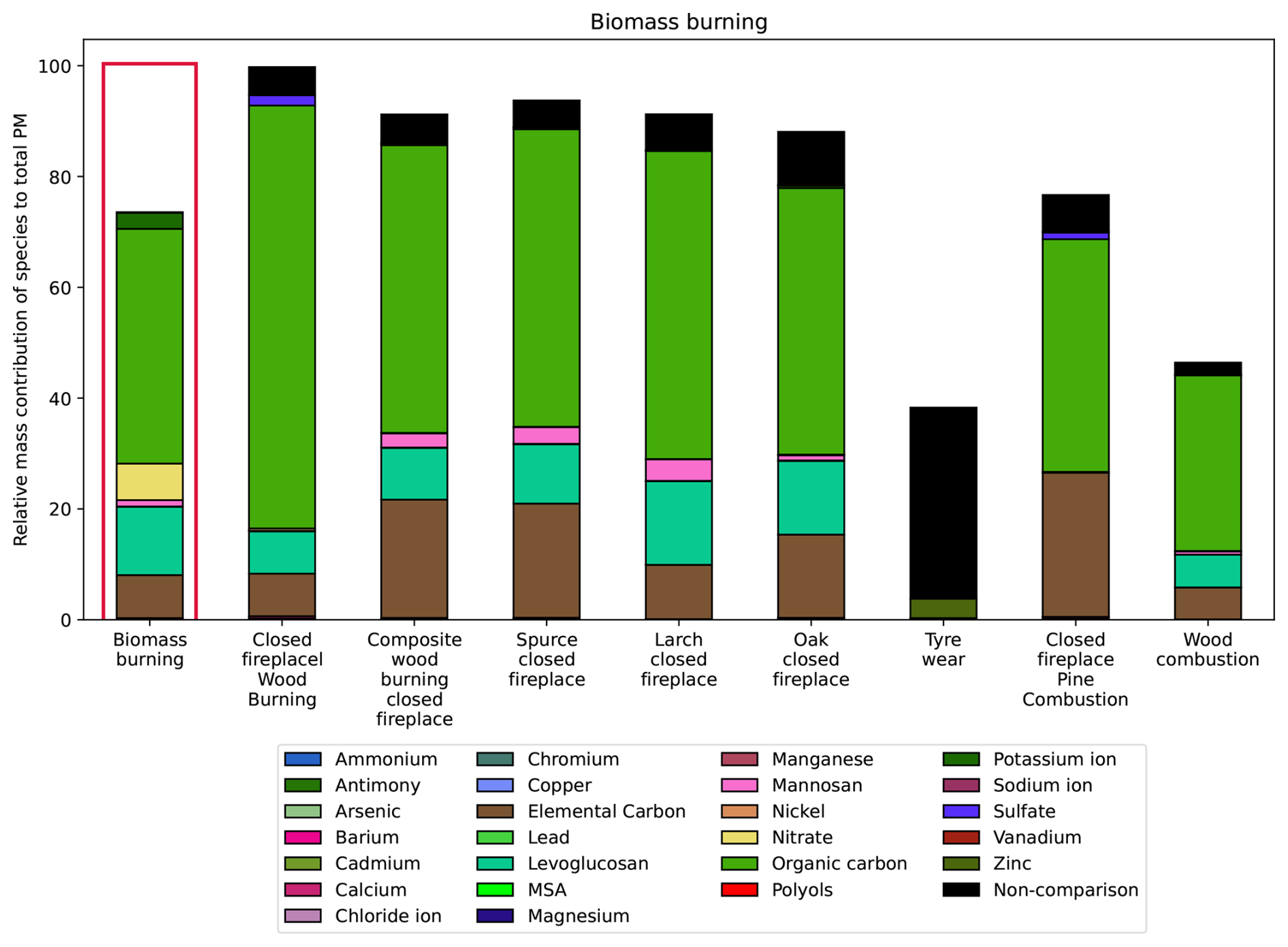
Figure 6 Composition of BB in Grenoble (framed in red) and its eight most similar sources extracted from SPECIEUROPE. The color denotes the chemical species. The y-axis is the mass of the given species relative to the PM total mass. Non-comparison is the total mass of the chemicals not used for the comparison.

In addition, the tool observed not only the PD and SID, but also the number of chemicals used for comparison, supposing that the comparison with less than half of the chemical species in the profile is insignificant. The outputs of this tool generate a list of sources whose chemical profiles are the most similar to the tested one (Fig. S7). Finally, the information about country and year tests, references, as well as the ratio between different chemicals in the profile is exported, providing complete information. The code also generates figures of the chemical composition of the profiles (like in Fig. 6) and PD-SID figures (like in Fig. S7), which allow the user to select the number of profiles that are the most similar to the tested one (eight profiles in the case of figure 6). The Python code for this tool is proposed in the same previous Python package as above and is presented in S1.

An example of using this tool is provided for the biomass burning (BB) factor of the same 11-factor base run of the Grenoble PMF used above. BB, is one of the most well-known sources in the database (76 biomass combustion profiles over a total of 287 profiles in SPECIEUROPE). Figures S7 and S8 present the PD-SID for the comparisons with SPECIEUROPE and SPECIEUROPE + IGE databases, respectively. Using the latter yielded a lower average of PD and SID compared to using only SPECIEUROPE (PD: 0.2 vs. 0.1, SID: 0.8 vs. 0.6). Indeed, the chemical profiles from the SPECIEUROPE database are barely used in the comparison of Fig. S8, which mainly uses profiles from France (included in the IGE database) due to their proximity, as reported by Weber et al. (2019). Only one chemical profile in SPECIEUROPE appeared in the comparison, which is the Larch closed fireplace. However, while using SPECIEUROPE led to a higher distance for the returned profiles, PD and SID remained within the homogeneous limits in both comparisons.

A closer examination of the composition used to compare the BB chemical profile in Grenoble and the eight most similar ones exported by the tool in the SPECIEUROPE is provided in Fig. 6. Most of the sources are related to wood combustion activities, with the main compositions of the source being OC, Levoglucosan, and EC. The “non-comparison” composition (total mass of the chemicals that were not used for the comparison) is relatively low (under 10 %), giving some confidence in the proximity of the profiles. Surprisingly, the “Tyre wear” source appears in this list of the most similar profiles to BB in Grenoble; however, the contribution of non-comparison species is 95 %, indicating the comparison did not consider the main composition of this source. Indeed, the species used for this comparison are mainly trace metals (Antimony, Arsenic, Barium, Cadmium, Calcium, Chromium, Copper, Lead, Magnesium, Manganese, Nickel, Vanadium, Zinc), which are not the proper tracers nor the high contributors to the BB source. Consequently, the number of species used to compare and the contribution of these species should be investigated to ensure the robustness of the comparison.

These results emphasize that it is crucial to consider the SID and PD values together with the number of chemical species compared, but also to observe in more detail the chemical profiles in order to evaluate the PMF solutions. Hence, with this added possibility of rapidly accessing these comparisons, this tool efficiently generates meaningful results in the process of performing a PMF study. However, it would be interesting to keep implementing more chemical profiles in the SPECIEUROPE database, and alternative methods like creating a joint database with SPECIATE (https://www.epa.gov/air-emissions-modeling/speciate, last access: 2 April 2025) could be considered.

These results emphasize that it is crucial to consider the SID and PD values together with the number of chemical species compared, but also to observe in more detail the chemical profiles in order to evaluate the PMF solutions. The output of the tool is a list of similar chemical profiles, which give an idea of the nature of PMF-derived sources. Other investigations, such as the characteristics of the sites, should be considered when identifying the source.

4 Conclusion

This study tries to establish a more robust methodology to minimize the subjectivity in performing source-receptor modelling using the Positive Matrix Factorization methodology. This provides to both the scientific community and first-time users with a reliable framework for obtaining accurate solutions. Through extensive testing, we identified key steps that mitigate subjectivity in the PMF model and proposed clear recommendations for tracer selection and PMF solution validation.

Tests performed on the input chemical species demonstrated that changes in input data does not significantly influence the PMF solution. With a disparity between OC and OC^∗ of less than 6 %, the PMF solution remained unchanged, suggesting that subtracting the carbon mass is unnecessary in this case. Furthermore, these tests point out that using a proper tracer, (i.e. emitted by a single source only) yields more accurate results than using several, improving source separation and reducing tracer dispersion across other sources.

In determining the optimal number of sources, we emphasized key criteria for tracer selection in source identification. Important criteria for a tracer to delineate a distinct source requires $S/N$ ≥ 3 and a quite independent temporal evolution (with R² between the tracer and the other chemicals in the input matrix lower than 0.3). Incorporating such a tracer in the PMF model enables the identification of a new source without distorting the chemical profiles of existing sources.

Finally, specific tools for PMF result validation were set up, including validation on key chemical ratios and comparisons with reference chemical profiles from archival databases. Comparing with well-known chemical ratios representative of a source helps in confirming that the chemical profile is appropriate, ensuring the main components contribute as expected. In addition, the test on comparing PMF-derived source and chemical profiles in SPECIEUROPE and IGE database enlightened the importance of considering not only SID and PD distances but also the number of species and the accuracy of mass reconstruction. These factors are crucial for reliable and meaningful comparisons.

Many tools used in this study have been integrated into a dedicated Python package – PMF_toolkits, providing the atmospheric science community with some more advanced and easy tools for PMF input preparation, source tracer selection, solution validation, and visualization. This contribution paves the way for more standardized and objective PMF analyses, ultimately enhancing source apportionment studies and air quality research.