Quantifying landcover-specific fluxes over a heterogeneous landscape through coupling UAV-measured mixing ratios with a large-eddy simulation model and Eddy-covariance measurements

Many natural ecosystems are composed of heterogeneous patches differentiated by wetness levels and vegetation composition, resulting in fine-scale flux patterns across the different landcovers that can be challenging to quantify. Here, we present a case study at Stordalen Mire in subarctic Sweden, where we conducted Uncrewed Aerial Vehicle (UAV) measurements of CO₂ mole fractions and combine them with a large-eddy simulation (LES) model through a site-level inversion method to differentiate the flux rate signatures from different patch types. We use the LES model EULAG (EUlerian LAGrangian) to simulate high-resolution flow patterns and benchmark the spatial variability of modelled concentrations with data from UAV-based grid surveys of CO₂ mixing ratio. Coupling the inversion results with eddy-covariance (EC) flux measurements for the time of the UAV flight allows quantifying net CO₂ fluxes for the individual landcover types. Model evaluation showed an R² up to 0.70, with model uncertainties mostly related to the transport model uncertainty and the UAV sampling footprint that does not evenly sample landcover types. The inversion fluxes were subsequently compared to patch-level chamber measurements of carbon dioxide from palsa, bog, and fen, and showed a good agreement in flux patterns across those patch types dominating the UAV-sampled footprint. Different landcover classification schemes were considered, and results showed a consistent improvement in the model performance when further representing the ecological and hydrological heterogeneities. Our novel technique shows promising results in estimating landcover-type flux heterogeneity within eddy-covariance tower footprints, thus providing a basis for upscaling of EC fluxes to a larger domain.

1 Introduction

Landcover heterogeneity plays a major role in modulating greenhouse gas (GHG) emissions from natural biomes, thus affecting the estimation of GHG emissions at the global and local scales (Desai et al., 2008; Ludwig et al., 2024; Premke et al., 2016). This heterogeneity is represented by spatial variability across ecological (e.g., vegetation type and composition), hydrological (e.g., wetness level, water depth, lateral flow), chemical (e.g., pH, salinity, soil properties), and microbial (e.g., microbial communities and corresponding niches) characteristics (Arsenault et al., 2019; Bohn et al., 2013; Hu et al., 2024; Kieckbusch et al., 2006; Oloo et al., 2016), the main drivers of the carbon dynamics and consequently carbon emissions (Cao et al., 2024; Li et al., 2024). Peatlands are one of the natural ecosystems exhibiting a high spatial variability that, in some cases, can result in patches with typical sizes of only up to few meters having strongly different biogeochemical fingerprints. This mosaic composition of wetlands results in heterogeneous patterns of greenhouse gas fluxes associated with the different patches forming a wetland (McNicol et al., 2017; Rey-Sanchez et al., 2018; Shahan et al., 2022), thus challenging landscape-scale quantification of landcover specific-fluxes and consequently model's estimations of such heterogeneous ecosystems (Bohn et al., 2013; Yazbeck and Bohrer, 2023).

Several measurement techniques can be implemented to quantify patch-level emissions of greenhouse gases. A common approach is to use flux chamber measurements (Pumpanen et al., 2004), where usually an episodic quantification of the flux from a specific patch is taken over an area hardly exceeding 1 m², noting that with the use of auto-chambers, extended timeseries of chamber measurement are possible (Bubier et al., 2003; Holmes et al., 2022). Chambers provide information on GHG flux rate variability across patch-types and they are useful for hotspot detection (Anthony and Silver, 2024; Ojanen et al., 2012). However, upscaling flux rates from plot level (0.1–1 m) to the whole patch-scale (100–1000 m) is challenging due to its relatively small spatio-temporal scales (Morin, 2019). On the other hand, eddy-covariance (EC) towers provide an estimate of flux rates at a larger spatio-temporal coverage allowing flux quantification over larger footprints through producing an effective net flux of the mixed landscape (Baldocchi, 2014). Although EC towers provide measurements at high temporal resolution, they cannot explicitly provide a direct quantification of the patch-level flux forming the underlying landscape (Chu et al., 2021; Matthes et al., 2014). Although several approaches have been implemented to upscale flux observations from chamber to EC footprint, bridging the gap between these different scales remains challenging (Fox et al., 2008; Simpson et al., 2019)

The emergence of Uncrewed Aerial Vehicles (UAVs) opened the door for new measurement possibilities with a potential of bridging this scaling gap. UAVs are commonly used for investigating landscapes at high spatial resolution, e.g., through grid surveys of hyperspectral and/or thermal imagery that can be used to derive indices for vegetation classification (Doughty and Cavanaugh, 2019; Zheng et al., 2022; Zhuo et al., 2024), or other surface properties; however, the use of UAVs is not restricted to imagery but includes meteorological variables like wind speed, temperature and gas mole fractions (Andersen et al., 2018; Bolek et al., 2024; Bolek and Testik, 2022; Kunz et al., 2018; Neumann and Bartholmai, 2015; Wildmann and Wetz, 2022). UAV platforms equipped with gas analyzers can effectively quantify emission rates from point sources such as power plants by employing mass balance or Gaussian plume inversion techniques, as they can capture the spatial variability of concentration enhancements at various downwind distances and altitudes (Andersen et al., 2018; Shah et al., 2020; Shaw et al., 2021). Given the potential of UAVs for surveying and monitoring small-scale spatial heterogeneity, integrating UAV measurements with EC tower data could enhance our understanding of flux variability within the tower footprint (Bou-Zeid et al., 2020; Giannico et al., 2018).

Nevertheless, UAV inversion could also be applied to infer patch-level and land surface fluxes. Mukhartova et al. (2024) present a theoretical framework and application for inferring the surface distribution of GHG fluxes over a complex vegetated terrain using a 3D hydrodynamic forward model linking UAV observations at two different heights to surface fluxes. Pirk et al. (2022) couple UAV profile measurements of temperature and relative humidity to a Large-Eddy Simulation (LES) model within a Bayesian optimization framework to infer surface heat fluxes, showing a good match with EC data. Wang et al. (2019) apply a top-down modeling approach coupled with a light-use efficiency model to UAV multispectral and thermal imageries to derive flux maps of Gross Primary Production (GPP) and evapotranspiration and other relevant variables. Other UAV-based approaches not involving inversion techniques but incorporating an eddy-covariance set-up showed a potential in estimating patch-type fluxes from heterogeneous landscapes (Pirk et al., 2024; Sun et al., 2021).

In this study, we leverage the UAV capability of sampling grid surveys of CO₂ model fraction through coupling it to high resolution transport modeling, like LES, and eddy covariance measurement to derive patch-level fluxes from a heterogeneous landscape. We derive a submeso-scale inversion that, after solving the steady state transport of a tracer emitted from a heterogeneous surface, uses UAV-measured CO₂ concentration to apply a linear optimization to derive scaling factors of patch-level fluxes. We couple these results with EC tower measurements of NEE in order to quantify flux magnitudes of each patch type. With this submeso-scale inversion, we need one high resolution simulation using an LES model and then perform the optimization on the time-averaged output, thus, reducing the computational resources usually associated with optimization frameworks. Although we apply this technique to a pilot project investigating CO₂ emissions from a northern peatland formed of a mixed patches of palsa, bogs, and fens, this method could be applied to other heterogeneous landscapes, and is therefore not necessarily restricted to wetlands.

2 Methodology

2.1 Study Site

The study site is the Stordalen mire, located in subarctic Sweden (68°21^′ N, 19°02^′ E). The site is characterized by sporadic permafrost and exhibits significant small-scale variation in soil moisture and vegetation types (Bäckstrand et al., 2010; Sjögersten et al., 2023). This thawing permafrost peatland is situated close to the shoreline of Lake Torneträsk and is encircled by small, shallow post-glacial lakes. It consists of elevated, drained palsa areas underlain by ice-rich permafrost, ombrotrophic wet bogs dominated by sphagnum moss, permafrost-free fens characterized by sedge vegetation, and open water ponds, both permanent and those formed more recently due to permafrost thaw (Varner et al., 2022). The average annual near-surface air temperature at the site is 1.0 °C and mean annual precipitation is approximately 330 mm yr⁻¹, while rising temperatures are expected to accelerate permafrost loss (Callaghan et al., 2013).

2.2 Field Measurements

A UAV-based set up is used to get grid surveys of CO₂ mole fractions within the area of interest, which is including the footprint of the local ICOS EC tower (see also below). The UAV carries a TriSonica Mini 2D anemometer for measuring wind characteristics along with temperature, humidity, and pressure. Additionally, a LI-850 analyzer was connected to the drone with the sampling inlet placed adjacent to the anemometer. The analyzer measures CO₂ mixing ratio with a 10 s averaged uncertainty of ± 0.36 ppm (Bolek et al., 2024). We use two grid-surveys of CO₂ mixing ratios taken in the course of a field campaign during 11–14 September 2023 at Stordalen mire (Bolek et al., 2024). The grid-survey was split into three areas as shown in Fig. 1, with each surveyed area sampled for about 14 min. The surveyed area is bounded by the Villasjön lake to the west, and includes heterogeneous patches of palsa, bog, and fens. The UAV was configured to maintain a constant speed while navigating a predetermined horizontal grid pattern at a constant altitude of 10 m. The survey began with flight paths aligned along the east-west axis, followed by north-south routes, ensuring that intersection points were sampled twice at different times. Given a flight speed of 4 m s⁻¹ and a sampling rate of 2 Hz, the spacing between each sampling point, represented by black circles in Fig. 1, was approximately 2 m. After filtering and despiking, the collected data in each area were aggregated into 10 spatial cells along both latitude and longitude, yielding a resolution of approximately 15–20 m. To refine the spatial representation, the averaged data were then interpolated using the ordinary Kriging method (Pereira et al., 2022). Further details about UAV data collection and processing can be found in Bolek et al. (2024).

Figure 1 (a) Landcover classification within the Stordalen Mire study area at a grid resolution of 2×2 m based on Varner et al. (2022). Panel (b) shows the UAV-surveyed area in Stordalen mire using a satellite image from © Google Maps. The yellow line delineates the three target areas, and the black dots correspond to the points surveyed by the drone. The red triangle shows the EC tower location on the map.

For the eddy-covariance data, we used data provided by the ICOS tower SE-Sto located in the center of the area of interest (Lundin et al., 2024). Palsa, bog, and fen patches are covered by the tower footprint. The measurement height is 2.2 m, and data of meteorological variables, energy and carbon fluxes is provided at half-hourly timestep. Chamber measurements of CO₂ fluxes from the different patches within the tower footprint were taken over the course of the growing season of 2023 during the months of May, July, and September. All measurements were taken during the daytime, mostly between 08:00 and 14:00 local time. The chamber footprint covers an area of 491 cm², the chamber hood had a height of 25 cm and was equipped with a fan, a probe for relative humidity and temperature probe, and a pressure sensor. An Aeris MIRA Ultra N₂O $/$ CO₂ gas analyzer was used for CO₂ concentration sampling. More information on the chamber measurements performed can be found in Triches et al. (2025).

2.3 Large-Eddy Simulation

In order to simulate the transport at the time of the UAV flight, we used the Large-Eddy Simulation (LES) model EULAG, the Eulerian/semi-Lagrangian fluid solver (Prusa et al., 2008). EULAG is a well-established numerical tool for simulating atmospheric dynamics across various scales. It is particularly suited for high Reynolds number and stratified flows under gravity (Piotrowski and Smolarkiewicz, 2022; Smolarkiewicz et al., 2014). The model solves a soundproof form of the Euler equations, incorporating conservation laws for dry mass, momentum, and entropy, using a semi-implicit integration scheme. This integrator utilizes the multidimensional positive definite advection transport algorithm (MPDATA) for atmospheric flows (Smolarkiewicz, 2006). To account for turbulence, the model solves a prognostic equation for Turbulent Kinetic Energy (TKE) and applies a dynamic Smagorinsky model, where eddy viscosity is parameterized based on TKE (Schumann, 1991; Sorbjan, 1996). EULAG has been extensively used as an LES model for statistical and applied studies (Englberger and Dörnbrack, 2017; Kilroy et al., 2024; Klonecki and Prunet, 2020; Schlutow et al., 2024; Strugarek et al., 2016; Wyszogrodzki et al., 2012; Ziemianski et al., 2021).

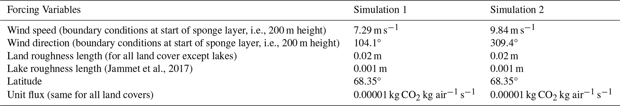
2.3.1 EULAG Forcings and Input

In our simulations, we use the Boussinesq approximation with cyclic boundary conditions. The domain size is $\mathrm{1024}\times \mathrm{1024}\times \mathrm{256}$ m³ with a resolution of $\mathrm{2}\times \mathrm{2}\times \mathrm{2}$ m³. A “moving sponge/absorber” is utilized at the top boundary, where a Rayleigh damping scheme is applied above 200 m. This scheme specifically affects the horizontal wind component, gradually adjusting the flow toward the geostrophic wind. The model is spun up for 12.5 h and an additional 30 min are run under steady state conditions, which are used for the analysis. We use the EC tower measurement for the time of the UAV flight to prescribe EULAG forcings. Using the same EC tower measurements, which provide the friction velocity u^* and the corresponding wind speed, we derive the input roughness length and wind speed at the upper boundary conditions. Heat flux is not included in the simulations as neutral conditions dominate the time of measurement of the UAV flight (based on the EC-derived Obukhov length). All patch types were identically prescribed with the same input flux of the simulated tracer as a starting condition. Table 1 includes all details of EULAG forcing input parameters.

Table 1 Input parameters and forcing conditions in EULAG.

2.3.2 Land cover configuration

We adopted the landcover classification published in (Varner et al., 2022). In this study, 8 main land cover types are defined: palsa (or hummock), semi-wet bog, wet bog, fen (wet graminoid), tall shrub, open water, rock, and others. Since the focus of this study is on carbon emissions, the landcover considered in our simulations are palsa, bog, lake, fen, and shrubs. Other landcovers are included in the study area, but with no flux emissions. The classification resolution is 2×2 m². The exact location of the simulated landscape was defined based on the wind direction (Fig. 2). In Simulation 1, where the wind is coming from the southeast direction, the map is defined so that the target area for flux quantification is at its northwest, thus, reducing the effect of cyclic conditions and taking into account the effect of upstream roughness and transport on the concentration fields within the sampled area. As for Simulation 2, the wind is coming from the northwest direction, thus, the map section is defined so that the target area for flux quantification is at its southeast.

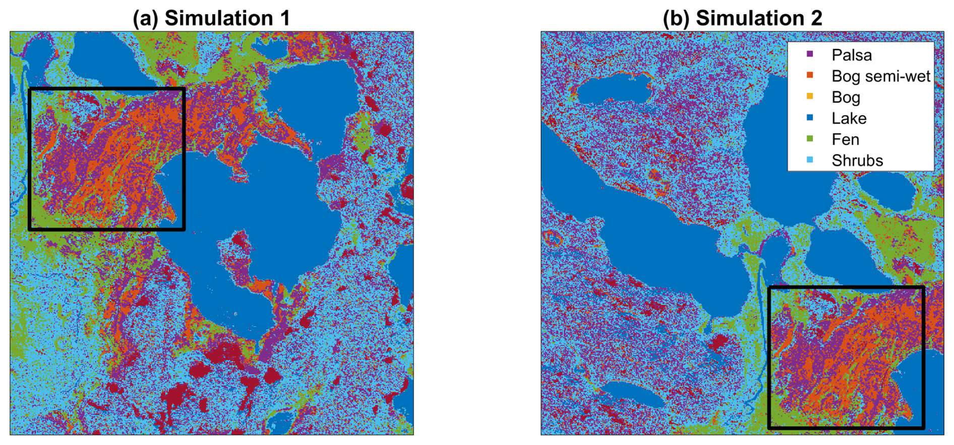
Figure 2 Input topographies for Simulations 1 (a) and Simulation 2 (b). The black box refers the area sampled by the UAV and corresponding to the section shown in Fig. 1.

In order to evaluate the configuration options of our setup, specifically the impact of adding more landcovers to the model, we run four EULAG simulations with different numbers of landcover types included, focusing on Simulation 1. The simulations will be labeled as “lc_3”, lc_4”, “lc_5”, and “lc_6” where lc_3 refers to the simulation with 3 landcover types, lc_4 for the simulation with 4 landcover types and so on. Table 2 includes the details of the classifications considered for the four different simulations and Fig. 3 shows the corresponding simulated landcover map for each simulation.

Table 2 Simulated landcover types for each of the four simulations, along with the corresponding land cover classifications from Varner et al. (2022), are included in each simulated landcover.

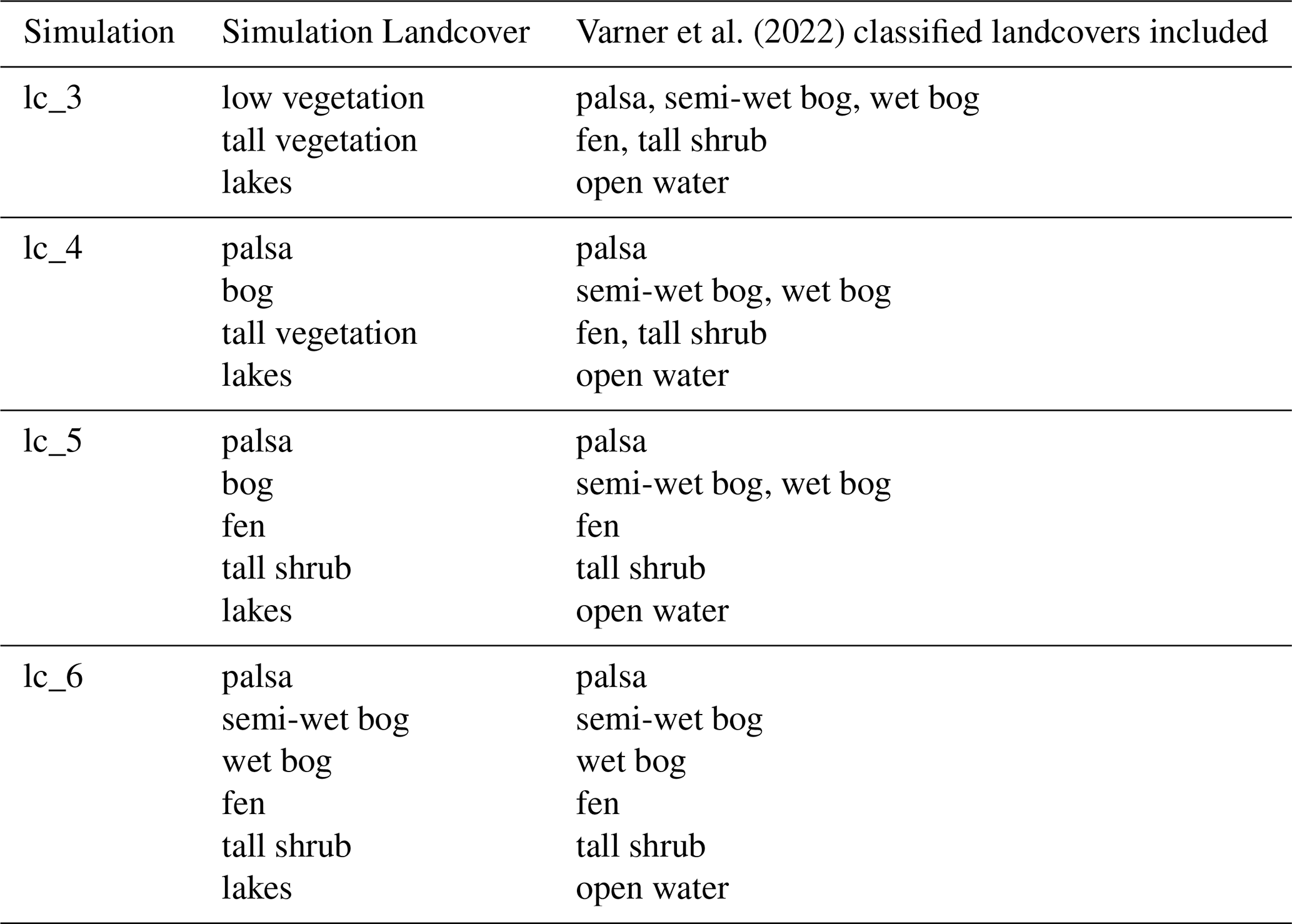
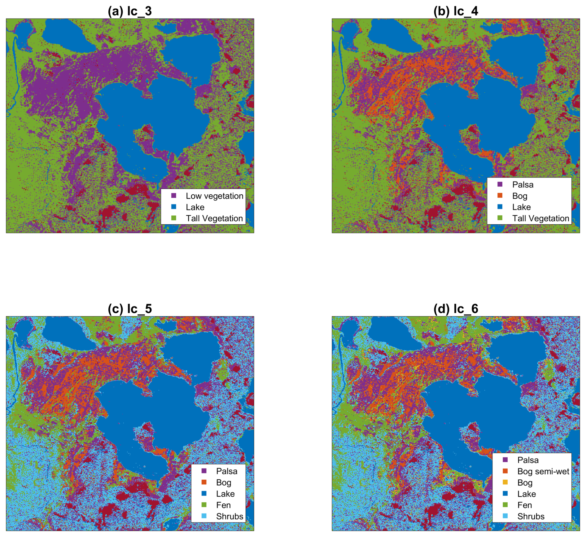
Figure 3 Landcover classification map used as input to EULAG for each of the different four different landcover configurations.

2.4 Submeso-scale Flux Inversion

2.4.1 Derivation

The submeso-scale inversion is applied on the 30 min averaged output of EULAG, after the model reaches a steady state, coupled with the UAV grid survey. The below equation lays down the assumption and derivation of the submeso-scale flux inversion. Equation (1) represents the transport equation for a Reynolds averaged inert (passive) tracer:

$$\begin{array}{}\text{(1)}& {\displaystyle \frac{\partial \stackrel{\mathrm{‾}}{C}}{\partial t}}+\mathrm{\nabla }.\left(\stackrel{\mathrm{‾}}{\mathit{u}}\stackrel{\mathrm{‾}}{C}\right)-\mathrm{\nabla }.\left(K\mathrm{\nabla }\stackrel{\mathrm{‾}}{C}\right)=\mathrm{0}\end{array}$$

on the domain Ω⊂R³ with flux boundary condition

$$\begin{array}{}\text{(2)}& -K{\displaystyle \frac{\partial \stackrel{\mathrm{‾}}{C}}{\partial z}}=Q\left(x,y\right)\text{on}\partial \mathrm{\Omega }\end{array}$$

where ∂Ω denotes the surface, i.e., all points (x, y, z) with z=z₀. $\stackrel{\mathrm{‾}}{\mathit{u}}$ is the Reynolds averaged wind, $\stackrel{\mathrm{‾}}{C}$ is the Reynolds averaged tracer concentration, t denotes time, K denotes the eddy diffusivity, and Q represents the surface flux. For brevity, we define the linear transport operator as

$$\begin{array}{}\text{(3)}& \mathit{T}\stackrel{\mathrm{‾}}{C}=\mathrm{\nabla }.\left(\stackrel{\mathrm{‾}}{\mathit{u}}\stackrel{\mathrm{‾}}{C}\right)-\mathrm{\nabla }.\left(K\mathrm{\nabla }\stackrel{\mathrm{‾}}{C}\right)\end{array}$$

Let $i=\mathrm{0},\mathrm{1},\mathrm{\dots }$ index the land cover classes ∂Ω_i, e.g., grass, shrubs, open water body, where each landcover or patch-type is associated with its own surface flux (unit of kg CO₂ kg air⁻¹ s⁻¹) as follows

$$\begin{array}{}\text{(4)}& Q_i\left(x,y\right)=\left\{\begin{array}{l}{\mathrm{10}}^{-\mathrm{5}}\text{ if }\left(x,y\right)\in \partial {\mathrm{\Omega }}_i\\ \mathrm{0}\text{else}\end{array}\right.\end{array}$$

With

$$\begin{array}{}\text{(5)}& \sum _i\partial {\mathrm{\Omega }}_i=\partial \mathrm{\Omega }.\end{array}$$

Thus, all points on the surface belonging to the same land cover class are associated with same surface flux. EULAG would solve the transport equation outlined in Eq. (1) with a boundary condition defined in Eq. (2) for individual tracers:

$$\begin{array}{}\text{(6)}& \begin{array}{rl}& \mathit{T}{\mathit{\phi }}_i=\mathrm{0}\text{ on }\mathrm{\Omega }\\ & -K{\displaystyle \frac{\partial {\mathit{\phi }}_i}{\partial z}}=Q_i\left(x,y\right)\text{ on }\partial \mathrm{\Omega };\end{array}\end{array}$$

where φ_i is the tracer associated with a specific landcover type. Since we are dealing with linear transport of passive tracers, we can construct the tracer field as a linear combination of the patch-level associated fields φ_i as follows:

$$\begin{array}{}\text{(7)}& \stackrel{\mathrm{‾}}{C}\left(x,y,z\right)=\sum _i{a}_i{\stackrel{\mathrm{‾}}{\mathit{\phi }}}_i\left(x,y,z\right)\end{array}$$

where a_i are scaling factors associated with each landcover. Multiplying Eq. (6) by a_i and summing over i leads to the below Eq. (8):

$$\begin{array}{}\text{(8)}& \begin{array}{rl}& \mathit{T}\stackrel{\mathrm{‾}}{C}=\mathrm{0}\text{on}\mathrm{\Omega }\\ & -K{\displaystyle \frac{\partial \stackrel{\mathrm{‾}}{C}}{\partial z}}=\sum _i{Q}_i\left(x,y\right)\text{ on }\partial \mathrm{\Omega },\end{array}\end{array}$$

which leads to expression for the surface flux in terms of the scaling factors

$$\begin{array}{}\text{(9)}& Q(x,y)=\sum _i{a}_i{Q}_i\left(x,y\right).\end{array}$$

If observations of concentration or mole fractions of the tracer are available, the scaling factors a_i may be computed from observations at points $\left(x_j,y_j,z_j\right)$ by minimizing the below cost function:

$$\begin{array}{}\text{(10)}& J=\sum _j{\left({\stackrel{\mathrm{‾}}{C}}_{\mathrm{Mod}}^j-{\stackrel{\mathrm{‾}}{C}}_{\mathrm{Obs}}^j\right)}^{\mathrm{2}}.\end{array}$$

Where ${\stackrel{\mathrm{‾}}{C}}_{\mathrm{Mod}}^j$ is the modeled averaged concentration and could be expressed as ${\stackrel{\mathrm{‾}}{C}}_{\mathrm{Mod}}^j={\sum }_i{a}_i{\mathit{\phi }}_i\left(x_j,y_j,z_j\right)$ and ${\stackrel{\mathrm{‾}}{C}}_{\mathrm{Obs}}^j$ is the observed averaged concentration at the points $\left(x_j,y_j,z_j\right)$. The resulting problem can be solved with the linear least square method, i.e., solving for a_i minimizing by J, noting that the Reynolds averaging can be realized with a temporal average. In the case of our application ${\stackrel{\mathrm{‾}}{C}}_{\mathrm{Obs}}^j$ are provided by the UAV grid surveys. EULAG provides ${\stackrel{\mathrm{‾}}{C}}_{\mathrm{Mod}}^j$ for all defined landcover or patch-types, each associated with the input flux. Subsequently, linear optimization is applied to optimize for a_i, and thus derive the landcover fluxes by multiplying the optimized value of a_i with the originally input flux Q_i.

2.4.2 Applied Inversion and Flux Quantification

From the EULAG output, we get the time-averaged φ_i over 30 min of steady-state simulation time at the same height as the UAV concentrations are provided. UAV concentrations are then converted from ppm to kg kg⁻¹ to be consistent with EULAG concentrations. EULAG domain has a different background concentration than ambient concentration during the UAV flight, however, that would not affect our method as this latter relies on the concentration variability driven by fluxes regardless of the difference in background concentration between EULAG and UAV. Therefore, we subtract the mean concentration from observed and modeled concentrations, respectively, in order to remove the effect of background concentration, which is different in both modeled and observed datasets. We apply linear optimization to Eq. (10) solving for the a_i. Then, Q_i values associated with each landcover type are derived by multiplying the unit flux that was originally input in EULAG (constant flux of 10⁻⁵ kg CO₂ kg air⁻¹ s⁻¹ in our case) with the optimized a_i.

Note that the derived Q_i fluxes cannot be compared with ground-based measurements of fluxes, whether it is chambers or eddy-covariance due to the difference in background concentrations between the field and the model. However, the relative value of the landcover or patch-level fluxes compared to the mean flux value should hold. Therefore, having a measurement of ecosystem-scale total flux (i.e., NEE for carbon fluxes) for the time of UAV flight would provide us with the field-based mean flux, which could be used to scale the modeled landcover fluxes. Note though that the EC tower footprint corresponds to a sub-section of the simulated domain, therefore, the domain-wide mean flux cannot be used for the flux scaling but it should be restricted to the area sampled by the EC tower. Therefore, in order to perform the scaling a footprint model is needed to determine landcover type contribution to the EC flux within the area sampled by the EC tower. Using the Kljun et al. (2015) footprint model coupled with the same landcover classification used to prescribe the model's landcover configuration (Varner et al., 2022), the contribution of each landcover type to the EC-derived flux is determined. The calculated landcover contribution is then used to get a modeled average flux weighted by the landcover contribution within the EC footprint. The relative value of the inversion-derived fluxes to this modelled weighted mean is coupled with the EC-derived fluxes to compute the quantitative value of each landcover type.

2.5 Inversion Uncertainty

In order to investigate if there is any bias or uncertainty associated with the optimization process, synthetic experiments were performed. The lc_5 set-up was run again with the only difference at the magnitude of input tracer fluxes, where random fluxes were assigned for each patch type instead of unit fluxes. The model was spun up according to the protocol described in Sect. 2.3.1. The output 30 min average concentrations were sampled at the location of the UAV-measurements and were considered as “observed” concentrations for the purpose of the synthetic experiment. Then, linear optimization was applied to the lc_5 original simulation (i.e., simulation with constant fluxes 10⁻⁵), and optimized fluxes were compared to the random fluxes that were initially prescribed to the synthetic experiment run. The output shows an exact match between both set of fluxes. We tried this approach at several heights and found that the match between prescribed and optimized fluxes holds as long as the analysis height is below the mixing height of the boundary layer. Thus, no uncertainty or bias is induced from the linear optimization process.

To get the statistical uncertainty associated with the model, the 30 min simulation used in the inversion was consecutively repeated over 20 times, thus obtaining an ensemble of the optimized fluxes per patch type. In other words, after running the 12.5 h of spin up, the model was run for 10 h where each half-hour was analyzed separately and is associated with a new set of fluxes, thus, resulting in an ensemble of 20 estimated fluxes per patch type. Therefore, the range of the optimized flux values per landcover type represents the model's uncertainty.

3 Results

3.1 Model Evaluation

To evaluate the model, we performed a linear regression between the UAV-observed and EULAG-modeled CO₂ concentration derived from the optimized scaling factors. The linear regression metrics are summarized in Table 3. For Simulation 1, the linear regression R² increased with the number of land cover classes, going from 0.52 to 0.70. The Root Mean Square Error (RMSE) computed from the observed and modelled concentrations decreased with increasing the number of land cover classes, where it ranged between 0.68 and 0.54 ppm. The Akaike Information Criterion (AIC) decreased with increasing the number of landcover types, thus, showing that increasing the number of simulated landcover types improve the model performance. Figure 3 shows the concentration fields as measured by the UAV and modelled by EULAG for the lc_5 set-up after accounting for the difference in background concentrations. Simulation 2 focused only on lc_5, and concentration evaluation results are shown in Figure 5 where the linear model R² is 0.62 and corresponding RMSE of 0.24 ppm.

Table 3 Model evaluation metrics summary: The R² of the linear regression between modelled and observed CO₂ concentrations, the respective Akaike Information Criterion (AIC) and corresponding RMSE are listed for different numbers of land cover classes.

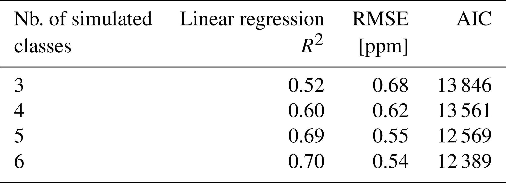
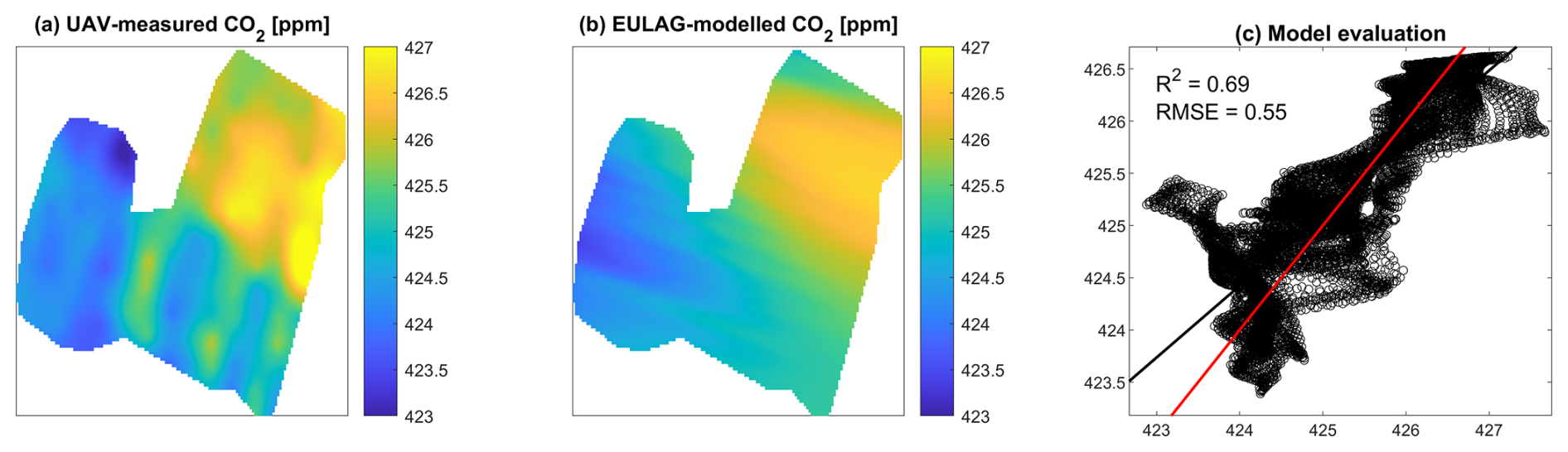
Figure 4 Evaluation of modelled CO₂ concentration fields at 10 m height for Simulation 1 corresponding to the lc_5 configuration. Panel (a) shows a grid survey of the observed concentrations as measured by the UAV, panel (b) the corresponding modeled total concentrations. Panel (c) plots the results of the linear regression applied to modelled concentration vs. observed concentration. It must be noted that here we removed the spatial-temporal average modeled concentration from the modeled concentration values and added the UAV-observed spatial-temporal average, thus, accounting for the difference in background concentrations, which is constant offset in this case. Concentrations are reported in ppm.

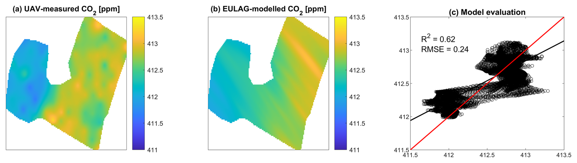
Figure 5 Similar to Fig. 4 but showing results for Simulation 2 corresponding to the lc_5 configuration.

Table 4 shows the optimized patch-level fluxes corresponding to each of the landcover configurations for simulations 1 and 2. For Simulation 1, the patch-level fluxes differ between the four simulations; however, some patterns are preserved across the simulations. For example, bogs are mostly acting as a carbon sinks, while fens and palsa are mostly a carbon source. Large flux variation between land cover setups is observed for palsa, bog, and fen, while a much smaller variability is observed at the level of lakes with a range of 1.87 to 4.08 µmol m⁻² s⁻¹, in addition of being a constant small source of carbon. A high flux is observed in lc_6 for wet bog, a consisting outlier for the set of flux values of the other patch-type and configurations. Simulation 2 fluxes show a different pattern than Simulation 1, where bog and shrubs are CO₂ sources, while palsa and fen are sinks. Lakes showed emissions in agreement with Simulation 1. Note that flux values for Simulation 2 are much smaller than fluxes for Simulation 1. This is due to the fact that EC-derived NEE is larger in terms of magnitude for Simulation 1 (NEE $=-\mathrm{3.29}$ µmol m⁻² s⁻¹) compared to Simulation 2 (NEE $=-\mathrm{0.33}$ µmol m⁻² s⁻¹), which will consequently affect the patch-level fluxes. Patch-type fluxes derived from this inversion could be used to construct a flux map showing the flux distribution over the surveyed area and around it as shown in Fig. 6.

Table 4 Optimized patch-level fluxes corresponding to the four landcover configurations. CO₂ flux unit is  µmol m⁻² s⁻¹.

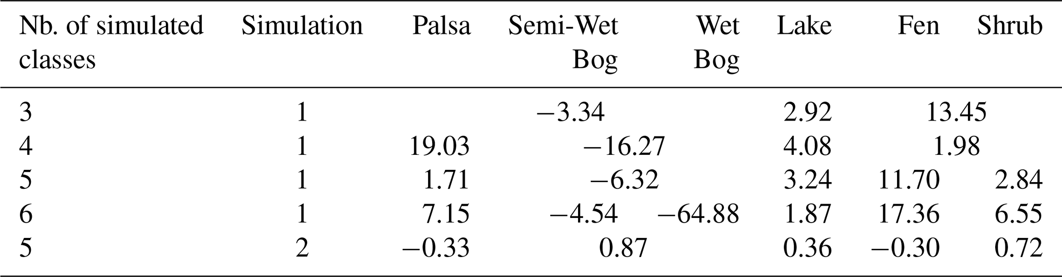
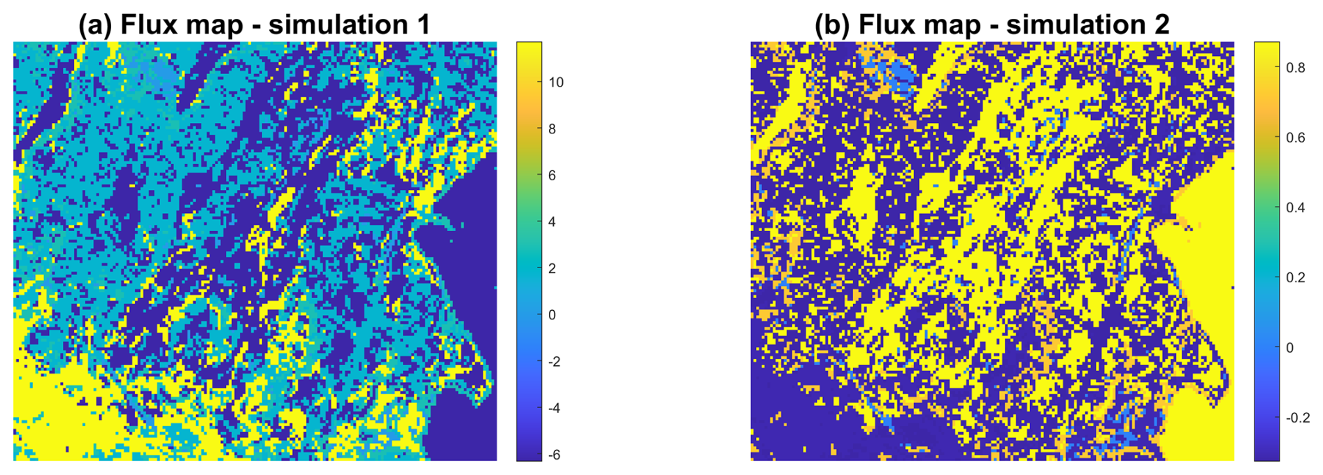
Figure 6 Flux map for the 5 classes landcover configuration for (a) Simulation 1 and (b) Simulation 2. Flux values are given in µmol m⁻² s⁻¹.

3.2 Model Assessment

We used chamber-measured fluxes from fen, bog, and palsa plots at Stordalen mire sampled during the same day of the UAV flight to assess the modeled flux estimations. Due to differences in spato-temporal scales between flux chamber measurements and inversion-derived patch-level fluxes, it is not meaningful to directly compare the flux values at pixel level. Therefore, we compared the flux patterns between different patches to the measured chamber fluxes for the same day of the UAV flight as shown in Fig. 7. The fluxes correspond to the lc_5 run, with their respective uncertainty constrained as explained in Sect. 2.5. The lc_5 configuration was considered as chamber measurements were split between fen, bog, and palsa, thus, matching the classification of lc_5. Flux estimation shows to have a wide range per patch-type, with palsa, bog, and fen fluxes showed a higher variability than the other landcovers (lake, shrubs). Still, some patterns are conserved across all the simulations, specifically bog being the main sink between the different patches and fen being a comparatively high source; however, palsa varied between being a source and sink. Regarding additional landcover classes not covered by flux chambers, lakes have mostly low fluxes with low variability, while shrubs showed to be a source of carbon with a couple of outliers of high flux estimations. Each of the 20 simulations shown in Fig. 7a has an associated R² value, corresponding to the R² of the linear regression between modeled and observed concentrations. The R² ranged between 0.62 and 0.72 for the 20 runs, where the flux values corresponding to the run with the highest R² showed the least variability in terms of flux values across the 5 different landcovers as shown through the black dots in Fig. 7a.

Chamber measurements for the day of the UAV flight for Simulation 1 show that most of the plots are a source of carbon, where fen and palsa are consistently emitting carbon across all sampled plots and bog is a lower source on average with few plots showing a slight sink of carbon. Note that all chamber measurements are consistently higher than the EC-derived NEE for the time of drone flight (Fig. 7b), thus, challenging any match between the inversion fluxes and chamber fluxes. As for Simulation 2, there is a match between the estimated fluxes and chamber-measured fluxes, noting that in this case the EC-derived NEE is more consistent with the chamber-measured values. The estimated fluxes for bog and fen are very close to the mean of chamber measurements, while fluxes simulated for palsa are underestimating the chamber mean. Thus, comparing both simulation fluxes to chamber data show a matching pattern between landcover fluxes but not for the three of them. For Simulation 1, a similar pattern is seen between bog and palsa but not for fen, while for Simulation 2 a similar pattern is seen between bog and fen but not for palsa.

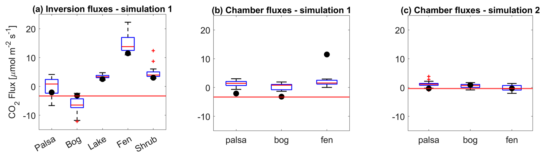
Figure 7 Comparison of inversion fluxes with chamber measurements taken the same day of the UAV flight. (a) The left panel corresponds to the ensemble of fluxes derived from the inversion of lc_5 set up corresponding to the inversion applied to 20 consecutive EULAG runs. The black dots represent the inversion fluxes corresponding to the run with the highest R² for the concentration linear regression. (b) The middle panel shows the range of chamber-measured fluxes for the day the UAV flight for Simulation 1, where the black dots correspond to the same dots as in panel (b). (c) The right panel shows the range of chamber-measured fluxes for the day the UAV flight for Simulation 2, where the black dots correspond to the inversion fluxes. CO₂ flux unit is µmol m⁻² s⁻¹. The red line in all panels represents the EC-derived NEE for the time of the UAV flight.

4 Discussion

4.1 Model Evaluation

The model evaluation shows good results in terms of linear regression between modelled and observed concentrations across all four different landcover classification, where R² ranged between 0.52 and 0.70. The additional degrees of freedom linked to an increased number of simulated landcover types led to an increase in linear regression metrics and decrease in RMSE, which is expected although the improvement in the model metrics differs between different scenarios, especially at the level of the AIC. This consistent trend in improved model evaluation metrics shows that having a detailed landcover classification leads to a better inversion, even when weighing the enhanced agreement between model and observations against the degrees of freedom in the optimization using the AIC. Going from lc_3 to lc_6, the split was mostly done based on different wetness levels. Low vegetation was split between palsa and bog, where bog is mostly wetter than palsa. Tall vegetation was split between shrub and fen, where fen is wetter than shrubs. Finally, in a last step bog was split between wet and semi-wet. Thus, this emphasizes the importance of accounting for the heterogeneity in wetness levels across the landscape for a better estimation of patch-level fluxes. This is mostly apparent through the AIC. The largest drop in the AIC happens when going from lc_4 to lc_5, i.e., splitting tall vegetation between shrub and fen, which have the biggest contrast in wetness levels, where fens are much wetter than shrubs. The lowest drop in AIC happens when going from lc_5 to lc_6, i.e., splitting the bog between wet and semi-wet, where the contrast wetness is not as strong as in the earlier cases. This wetness contrast is coupled in an ecological contrast, where wet and semi-wet bogs correspond to the same or similar vegetation type while shrubs correspond to a different vegetation type. Although the AIC is a relative indicator, the corresponding decrease trend across different configurations could be an indicator of the impact hydrologic and ecological heterogeneity plays when quantifying patch-level fluxes.

4.2 Flux Assessment

Comparing lc_3 to lc_6 fluxes, we see that splitting the low vegetation areas into separate (palsa/bog) patches resulted in a higher sink strength in bogs, compared to palsa, which agrees with the chamber measurements showing similar patterns in Fig. 7b. Similarly, splitting tall vegetation into fen and shrub shows that fens are a strong source for carbon, while shrubs are a smaller source with a range of estimated fluxes close to the palsa fluxes (Fig. 7a). Note that, based on the Varner et al. (2022) classification, palsa and shrubs are both considered types of palsa, thus sharing similar net CO₂ emissions characteristics. Also, when palsa and bog are simulated as one combined landcover class (lc_3), the resulting flux is a sink, which agrees with the coarse classification of this scenario where most of the palsa/bog area is labeled a bog, thus, the resulting flux would be mostly a sink of CO₂. Lake fluxes show the lowest uncertainty compared to other patch-types, with an estimated flux ranging between 1.87 and 4.76 µmol m⁻² s⁻¹. A study summarizing EC flux measurements taken over the same lake in Stordalen over the years 2012–2014 by Jammet et al. (2017) reports a range between −1.5 and 1.5 µmol m⁻² s⁻¹ for the ice-free season. Taking this range as a reference, our estimations appear to be slightly over-estimating lake emissions. The optimized fluxes show that fens are acting as a source while palsa and bog are mostly a sink, which might be unexpected as fens usually take up more carbon through photosynthesis than bogs (Holmes et al., 2022); however, a similar pattern is seen in the chamber measurements (Fig. 7b), where fens represented higher emissions than bogs, thus agreeing with the emissions of the time of UAV measurement. This might be related to the fact that our experiments took place at the end of the growing season, when fens could experience positive fluxes during the day time (Holmes et al., 2022).

For Simulation 1, there is a partial agreement in flux patterns between optimized fluxes and chamber fluxes, but in terms of absolute values, there is a mismatch in the flux range that varies between landcover types. For example, for palsa the inversion-estimated flux range is between −6.65 and 4.13 µmol m⁻² s⁻¹, while the chamber flux range is between −0.64 and 3.05 µmol m⁻² s⁻¹; however, for fen there is a large mismatch between the ranges, where the inversion fluxes range between 10.94 and 22.26 µmol m⁻² s⁻¹, while chamber data have a range of 0.04 and 2.95 µmol m⁻² s⁻¹. Although the spatial scale mismatch between chamber plots and whole patch-level flux footprint contributes to the difference observed in flux values, there are other factors that contribute to this mismatch as well. One of these factors is the composition of landcover patches within the domain surveyed by the UAV. Although the grid survey depicted in Fig. 1 is underlain by all simulated landcover types except lakes, this area is mostly covered by palsa and bog and is downwind of the lake bordering the mire from the east. As a consequence, very little impact from fen areas is captured by the UAV-surveyed mixing ratio, which could be one of the main reasons why fen fluxes are not well-constrained in the inversion and probably over-estimated. Similarly, this could be the reason why in the lc_6 configuration the sink strength in wet bogs is over-estimated – even though it is common to see high sinks for CO₂ in wetter bogs (Sulman et al., 2010), our estimated flux value is probably unrealistically large. This is probably due to the fact that wet bogs are poorly represented within the UAV-surveyed area, and associated patch sizes are small so that this land cover type never dominates a single UAV observation footprint. Although the lakes are not directly surveyed by the UAV, their impact on the measured mixing ratio is well-captured by the UAV as it is located directly upwind of the surveyed area, thus, resulting in much closer values to previously observed fluxes from the lake as discussed earlier. Simulation 2 showed a better match between chamber-measured fluxes and inversion fluxes, where for the three patch types the estimated fluxes fell within the range of measured fluxes, where fen and bog flux estimation through inversion are matching the mean of the chamber measurements fluxes. This is primarily due to the better agreement between EC- and chamber derived fluxes, so low EC-derived NEE flux also led to low fluxes from the inversion that matched the chamber results very well.

4.3 Model Uncertainty

Figure 7a shows a large variability across patch types: palsa is estimated to have a median flux of 0.83 µmol m⁻² s⁻¹, bog −6.46 µmol m⁻² s⁻¹, lake 3.35 µmol m⁻² s⁻¹, fen 13.80 µmol m⁻² s⁻¹, and shrubs 3.94 µmol m⁻² s⁻¹. However, for lc_5 where 20 simulations were performed, the simulation corresponding to the largest R² (0.72) and lowest RMSE (0.53 ppm) for the concentration linear regression had the least variability of fluxes between patch type where flux estimation are as follows: palsa is −2.08 µmol m⁻² s⁻¹, bog is −3.17 µmol m⁻² s⁻¹, lake is 2.54 µmol m⁻² s⁻¹, fen is 11.48 µmol m⁻² s⁻¹, and shrubs is 3.01 µmol m⁻² s⁻¹ (black dots in in Fig. 7a). This comparison shows that the optimized fluxes reported in Fig. 7a are probably over-estimating the absolute value of the fluxes. Several sources of uncertainty exist that could bias our flux estimations. Most prominently, there is the uncertainty related to the LES modeling of the tracer transport (Lucas et al., 2016; Zhang, 2021), especially since the synthetic experiment showed that no uncertainty is associated with the linear optimization (Sect. 2.5), in addition to the uncertainty that could arise from the steady-state assumption on which the inversion derivation is based upon.

LES does resolve the turbulent transport but assuming steady state and applying inversion on the temporally averaged concentration implies losing a lot of the turbulent transport information. This effect could be depicted in Figs. 4 and 5 when comparing the modeled and observed concentration fields. Although the model is capturing the overall variation in the concentrations, it is missing the small-scale turbulent effect captured by the drone and not represented in our model, like in the case of the horizontal vortices shown Fig. 4a and not represented in Fig. 4b due to the 30 min averaging. In the context of modeling wind flow and turbulence for the time of the UAV flight, LES provides a solution of the turbulent transport field that agrees with measured meteorological conditions which are then used to force the model (Table 1); however, it is not necessarily the transport field that was present at the time of UAV flight. Thus, each LES post-spinup 30 min run represents one potential solution, and not the truth, which results in the flux uncertainty of Fig. 7a. In addition, LES models resolve the larger, energy-containing turbulent eddies directly, while smaller sub-grid scale (SGS) eddies are approximated using a parameterization. The accuracy of LES depends on grid resolution – finer grids capture more turbulence but increase computational costs, while coarser grids rely more on SGS models, introducing potential errors. Uncertainties arise because SGS models approximate rather than resolve small-scale turbulence, leading to errors that can propagate to larger scales. These uncertainties affect the accuracy of transport modeling, thus influencing predictions of tracer concentrations, in our case CO₂.

Other sources of uncertainty could arise from the landcover classification considered in this study and the UAV measurements, although they both showed to have low errors associated with them: for the land cover, Varner et al. (2022) report 0.4 % a misclassification rate for the landcover classification, while Bolek et al. (2024) report an uncertainty less than 0.36 ppm for UAV measurements. Other sources of uncertainty arise from the errors associated with the EC measurement of NEE and the footprint model, although these errors would not affect the inversion-derived fluxes, but the computation of the quantitative flux values. This comprises, for example, the errors associated with the EC instrument noise, calibration drift, and data processing methods, as well as from the footprint model, which introduces uncertainty through assumptions about atmospheric stability, turbulence, and the spatial representation of flux contributions from heterogeneous surfaces. Uncertainty is also associated with chamber measurements used to compare the derived fluxes with, which can be affected by issues such as leakage, pressure effects, and alterations of the natural microclimate inside the chamber during sampling time.

Through this inversion approach, it is challenging to provide a value for the uncertainty in the flux estimations as we do not have a patch-level scale measurement of the fluxes to compare our data with. Nevertheless, assessing the mismatch between modeled and observed concentrations provides an estimate of the model uncertainty, where the lc_5 simulations result in 95 % confidence interval of 1.08 ppm for Simulation 1 and 0.47 ppm for Simulation 2.

4.4 Limitation, Applications, and Outlook

A limitation of this study is the relatively small number of land cover classes, which introduces the “aggregation error”. To address this, future work could substantially increase the number of unknowns (i.e., classes) and incorporate “a priori” information – such as wetness, nutrient status, microtopography, or specific vegetation types – to better constrain the problem. A promising direction would be to move away from rigid, predefined landcover classes. A simple first step could involve subdividing existing landcover categories into smaller sectors and optimizing each separately. A more advanced approach might optimize pixel-by-pixel, perhaps incorporating spatial correlation length scales, followed by post hoc analysis to identify coherent clusters – and assess whether they align with the predefined structure. Implementing such strategies would require more extensive data, potentially including tailored UAV campaigns to provide balanced coverage across the mire, in addition to extensive computational power, especially if models like LES are involved, however, simpler transport models could be explored as this study relies on the steady state assumption.

This small-scale inversion opens the door to further coupling UAV and EC measurements to derive patch level fluxes both within the EC tower footprint and in the surrounding landscape. Based on the inversion fluxes, it is possible to get the net carbon flux from larger areas, i.e. extrapolate measurements within the EC footprint area to the full mire area without having to assume matching land cover fractions in both domains. Since Simulation 1 has a SE wind, we use the Simulation 1 fluxes to get the net flux from the bog area surveyed by the drone (right two sections in Fig. 1b), while we use Simulation 2 fluxes to get the net flux from the palsa area (left section in Fig. 1b) as the wind is coming from the NW in this case. Using the lc_5 configuration, we get a net flux of −1.45 µmol m⁻² s⁻¹ for Simulation 1 and a net flux of 0.18 µmol m⁻² s⁻¹ for Simulation 2. Note that the EC-derived NEE for the same time of the UAV flights is −3.29 and −0.33 µmol m⁻² s⁻¹, respectively. The mismatch between the EC-derived NEE and the whole-area-derived NEE emphasize the role the small-scale heterogeneity and tower footprint play when deriving total net fluxes of carbon, noting that this inversion technique could be leveraged in upscaling studies using EC-derived fluxes to derive landscape-wide fluxes.

By applying this method during different periods over the course of the growing season, i.e., through flying the drone several times over the growing season, we could get a larger set of the patch-level fluxes that could be integrated over the whole growing season and result in season-long patch-level flux. In this study relying on just a couple of flights, we are able to estimate fluxes corresponding to the UAV flight time and/or any other time within similar meteorological and phenological conditions. Extending the results to represent patch-level carbon budgets for a full growing season is thus challenging; however, with further implementation of UAV flights within the EC tower footprint, patch-level carbon budgets could be possible. . In this case getting UAV measurements over different time of day is important to get patch-level flux contributions across different daytime conditions, notably nighttime conditions, although running LES under stable conditions could be challenging due to weak turbulence and strong stratification. It must be mentioned that this method would require a considerable amount of computational resources for running high-resolution models like LES; however, simpler transport models could be considered especially when averaged transport processes for steady-state conditions are assumed. The uncertainty coupled with the flux estimation could be overcome by increasing the drone surveyed area to better represent the effect of all landcover on the measured mixing ratio. Note that the UAV-LES inversion presented in this study could be applied to any flux tower as long drone measurement and landcover classification are provided, and is not limited to arctic or peatland ecosystems.

5 Conclusions

Through a combination of LES modeling, gridded mixing ratio observations from a UAV platform, a landcover classification, and Eddy covariance measurements, patch level CO₂ fluxes at 2×2 m resolution could be derived from a structured sub-Arctic mire. Distinct flux signatures could be assigned for pre-assigned land cover types, separating sources and sinks, and deriving flux rates differing by more than one order of magnitude between landscape elements. Evaluation of the modeled concentration fields showed a good match with UAV observations of atmospheric CO₂ concentrations, while assessment of the inversion flux rates through comparing them to flux chamber datasets for the same day of UAV flight showed an agreement in flux patterns between derived patch level fluxes and corresponding chamber fluxes, mostly for bog and palsa, the main landcover within the UAV sampled area footprint. This inversion technique opens the door for deriving patch-level fluxes from EC data, while bridging the scaling gap between patch-level fluxes (usually measured with chambers) and plot-level fluxes, thus suggesting a new method to upscaling to EC-derived fluxes to footprints larger than the EC tower footprint.