Impact of lower atmospheric scattering on ground-based optical thermospheric wind observations with spatially uneven airglow

Scattered airglow emissions in the lower atmosphere can bias ground-based interferometer observations of thermospheric winds, particularly when airglow brightness becomes spatially uneven due to auroras. During two geomagnetic storms with visible auroras on 10 May and 10 October 2024, the Doppler Asymmetric Spatial Heterodyne (DASH) and Fabry-Perot (FP) interferometers concurrently detected atypical winds at Siziwang (SIZW, 41.83° N, 111.93° E), suspected to be caused by scattering. These atypical winds, characterized by horizontal differences exceeding 400 m s⁻¹ between opposite cardinal directions (N-S or E-W) and downwelling exceeding 100 m s⁻¹, showed a strong temporal association with airglow brightness. By modelling the transmission of scattered airglow emissions, we calculate post-scattering wind speeds as the initial wind speeds weighted by both scattered and direct intensities. With fixed initial winds (100 m s⁻¹ westward, 400 m s⁻¹ southward, zero vertical wind), the simulation reproduces horizontal differences of approximately 400 m s⁻¹ on 10 May and 100 m s⁻¹ on 10 October, both capturing the temporal characteristics of the atypical winds. The simulation shows that scattering-induced biases on line-of-sight speed take their sign from the brighter region, while their magnitude varies directionally with the angle to that region: at 45° elevation, biases 135–180° azimuth away exceed those in the brighter region by more than 10 times. Limited by uncertainties in airglow images and optical depth of model inputs, the simulation incurs numerical errors of roughly 75 % during some periods. Effective correction of the scattering impact will require improved accuracy of model inputs in the future.

1 Introduction

Optical interferometers are widely utilized to observe thermospheric neutral wind (Burnside et al., 1981; Burnside and Tepley, 1989; Killeen et al., 1995; Emmert et al., 2001; Fejer et al., 2002; Emmert et al., 2006; Wu et al., 2014). Thermospheric wind can be derived from measuring the Doppler shift of OI red-line airglow emission at 630.0 nm. This emission, primarily from the collisional deactivation of O(¹D) generated by O${}_{\mathrm{2}}^{+}$ dissociative recombination, peaks near 250 km altitude. The height-integrated thermospheric wind around the peak altitude can be obtained (Biondi and Feibelman, 1968; Hernandez and Roble, 1976; Burnside et al., 1981; Biondi et al., 1995; Nakajima et al., 1995). For scanning interferometers, three-dimensional wind vectors can be derived by observing the zenith and four cardinal directions at a specific elevation angle. The scanning range covers a circular area about 500 km in diameter at airglow altitude. Given thermospheric wind uniformity at this scale, horizontal winds observed in two opposite cardinal directions (N-S or E-W) are typically similar. Averaging opposite cardinal directions improves accuracy, mitigates cloud effects, and is typically used to represent local meridional or zonal winds even during geomagnetic storms (Friedman and Herrero, 1982; Fejer et al., 2002; Sakanoi et al., 2002; Dhadly et al., 2017; Huang et al., 2018; Xu et al., 2019; Li et al., 2023; Wang et al., 2025).

However, horizontal winds in opposite cardinal directions occasionally show significant separation exceeding 100 m s⁻¹ and strong vertical winds, deviating from typical thermospheric wind uniformity. These observations often occur near auroras, unaffected by clouds or moonlight, and have acceptable standard errors. They mainly occur in polar regions (Crickmore et al., 1991; Price et al., 1995; Smith and Hernandez, 1995; Innis et al., 1999; Ishii et al., 2001; Guo and McEwen, 2003; Anderson et al., 2012), but have also been seen at mid-latitudes during major geomagnetic storms (Hernandez and Roble, 1976; Makela et al., 2014).

Atmospheric scattering of airglow emissions is thought to be one of the factors that biases ground-based wind observations, potentially accounting for the atypical wind. Initially, it was thought to impact airglow peak height measurements by photometers (Ashburn, 1954). Subsequent studies by Abreu et al. (1983) explored its impact on thermospheric wind speed measurements using a Fabry-Perot interferometer. Harding et al. (2017a, b) later systematically modelled and estimated these effects, revealing that scattering was responsible for the anomalous vertical winds observed at mid-latitudes during geomagnetic storms by Makela et al. (2014). Light from brighter airglow regions scatters omnidirectionally in the lower atmosphere, primarily the troposphere and stratosphere, and is detectable outside its original direction. The additional Doppler shift of this scattered light can bias the retrieval of line-of-sight (LOS) speeds as well as the converted horizontal and vertical winds. Harding et al. (2017b) also investigated the impact of atmospheric scattering on interferometer wind and temperature measurements during quiet periods.

Scattering-induced biases are more pronounced during spatially uneven airglow brightness, such as during auroras (Harding et al., 2017a). Uneven airglow brightness refers specifically to inhomogeneous red-line emissions. At mid-latitudes, marked uneven red-line airglow usually comes from red aurora. Despite their distinct origins, the spectral and altitudinal overlap of airglow and aurora will let ground-based optical instruments conflate the two. For red-line observations, the aurora itself may also bias the derived winds. Aurora could elevate the red-line emission profile (Kataoka et al., 2024b), so the interferometer samples winds that are both higher and farther away. This makes the northward view sense winds deviate from the expected thermospheric wind at 250 km altitude when looking toward the aurora. Additionally, spectral contamination from precipitating energetic ions could also bias interferometers (Makela et al., 2014). They suggested that the enhanced downwelling at mid-latitudes during storms might result from the contamination of the spectral profile by fast O atoms associated with the influx of low-energy O⁺ ions.

From a dynamical perspective, wind differences in opposite cardinal directions are considered horizontal divergence, which are often associated with changes in vertical winds. Near the aurora arc, these atypical winds are mainly caused by ion drag, Joule heating, and energy particle precipitation (Hays et al., 1984; Rees et al., 1984; Conde and Smith, 1995; Conde et al., 2001; Anderson et al., 2012). Generally, excessive horizontal divergence and vertical wind appear alongside rapidly changing auroras and exhibit a matching spatial relationship that upward (downward) winds accompanied by divergences (convergences) are often detected when aurora exists equatorward (poleward) of the observatory (Ishii et al., 2001; Guo and McEwen, 2003). The combination of vertical wind and horizontal divergence is related to gravity waves excited by the above processes in polar regions, presenting a wave-like structure and phase delay between vertical and horizontal wind components. (Price et al., 1995; Smith and Hernandez, 1995; Ishii et al., 1999, 2001; Shinagawa and Oyama, 2006). At mid-latitudes, which are not primary regions for magnetospheric energy injection, atypical winds are instead related to the propagation of gravity waves from polar regions (Hernandez and Roble, 1976).

During two geomagnetic storms on 10 May and 10 October 2024, with visible auroras, we observed similar atypical winds in ground-based interferometers at Siziwang (SIZW, 41.83° N, 111.93° E), China. These winds showed intense differences over 400 m s⁻¹ in two opposite cardinal directions for both meridional and zonal components, along with downward wind exceeding 100 m s⁻¹. The observations were unaffected by moonlight or clouds, and the interferometer retrieval errors were acceptable (see Sect. 3.1). These atypical winds at SIZW only occurred with auroras statistically and significantly deviated from the regional climatological norms over the China region (Jiang et al., 2018; Yang et al., 2020). This raises the question of whether the atypical winds arise from dynamical processes, are influenced by red aurora, or stem from scattering-induced biases and other measurement-related factors. Unfortunately, most of these mechanisms could amplify the wind-speed contrast between opposite cardinal directions, rendering them difficult to disentangle (Harding et al., 2017a). Given the scarcity of additional thermospheric-wind or auroral instruments, we remain unable to quantify every potential mechanism. Motivated by the observed phenomena, this study attempts to estimate how scattering modulates the atypical winds in these storms. While prior studies focus on vertical wind biases of Fabry-Perot interferometers under auroral conditions (Harding et al., 2017a, b), we will analyze the formation and patterns of horizontal differences caused by scattering. We will also incorporate Doppler Asymmetric Spatial Heterodyne (DASH) interferometer data to compare scattering impact across different interferometer types. As red auroras now regularly appear at the low magnetic latitudes of Japan and China during elevated solar activity (Kataoka et al., 2024a, b; Ma et al., 2024), a deeper understanding of scattering-induced biases is essential for the proper use of interferometer data collected in these regions. In the following text, a scattering radiative transfer model is used to simulate interferometer observations in two cases with visible aurora. The presence and patterns of scattering-induced biases are analyzed by comparing simulations with observations.

2 Instruments and model

This study was conducted at the Siziwang station (SIZW; 41.83° N, 111.93° E, and 37.7° N MLat) of the Chinese Meridian Project Phase II (Wang et al., 2024), utilizing a Dual-Channel All-sky Airglow Imager (DCAI), a Dual-Channel Optical Interferometer (DCOI), and a Fabry-Perot Interferometer (FPI). DCOI derives neutral winds by observing atomic oxygen green-line (557.7 nm, around 96 km) and red-line (630.0 nm, around 250 km). DCAI observes hydroxyl (around 87 km) and atomic oxygen red-line nightglow, respectively. FPI only works at the red-line. Our focus is on the red-line channel. Using DCAI images as one of the inputs, wind biases from optical interferometers can be simulated by a scattering radiative transfer model (scattering model for short). Instruments and the model are described in the following subsections.

2.1 Dual-Channel All-Sky Airglow Imager

Dual-Channel All-Sky Airglow Imager (DCAI) comprises a fisheye lens with an approximate 170° field of view, a 2 nm narrow-band filter, and a 1024 × 1024 pixel, 16 bit cooled CCD. DCAI exposure time of the red-line is 2 min. The obtained airglow images are first calibrated to the local spherical coordinate system, then sequentially corrected for stray light, Van Rhijn effect, and atmospheric extinction, and finally projected onto the 250 km airglow plane. Due to DCAI not calibrating the Rayleigh unit (Shiokawa et al., 2000), observed brightness is only normalized to the full-well value. And because of fish-eye lens distortion and the lack of Rayleigh unit calibration, the edge brightness of the view is inaccurate. Thus, observations are restricted within a 70° zenith angle. For larger zenith angles, the brightness is obtained by radial zero-order extrapolation in airglow projection. Detailed image processing procedures are in Appendix B.

2.2 Dual-channel optical interferometer

Dual-channel optical interferometer (DCOI) is a scanning interferometer using Doppler Asymmetric Spatial Heterodyne (DASH) technology. DASH exhibits a wider field of view, better thermal stability, simplified mechanisms, and lower tolerance requirements than other interferometer structures (Englert et al., 2007, 2010; Harlander et al., 2017; Wei et al., 2020). DCOI consists of a 630 nm narrow-band filter (2 nm bandwidth), a 9° field-of-view lens (f/6), a DASH interferometer with a 25 mm aperture, a Neon lamp for calibration, and a 2048 × 2048 pixel CCD (13.5 µm per pixel) (Wei et al., 2020; Zhu et al., 2023; Liu et al., 2025). Its thermal stability is maintained within 0.1 K. DCOI measures three-dimensional wind speeds by scanning five directions (zenith and four cardinal directions at 45° zenith angle). Each direction is exposed for 5 min, completing a cycle roughly every 25 min. DCOI adopts an observation with the smallest error after evening as the reference zero wind speed. The slant LOS speeds are subtracted by the time-regressed projection of vertical speed and then converted to horizontal using the sine of zenith angles. It is worth noting that during auroral events, vertical winds with absolute values exceeding 50 m s⁻¹ are excluded from the regression, as they contain scattering effects that could introduce additional biases to other directions. DCOI provides two series of meridional wind, two series of zonal wind, and one series of vertical wind.

2.3 Fabry-Perot Interferometer

Fabry-Perot Interferometer (FPI), as a mature solution, conducts comparative observations with DCOI. It features a 630 nm narrow-band filter (2 nm bandwidth), a 2.54° field-of-view lens (f/6), a 50 mm aperture etalon with a 7 mm gap, a frequency-stabilized laser for calibration, and a 1024 × 1024 pixel CCD (13 µm per pixel). FPI uses the same integration time and scanning method as DCOI to obtain horizontal and vertical winds for each cardinal direction and zenith. Details and historical results of FPI are in these references (Yuan et al., 2010; Wu et al., 2014; Yu et al., 2014; Huang et al., 2018; Jiang et al., 2018).

2.4 Scattering radiative transfer model

The model for estimating scattering impact is based on the scattering radiative transfer model and numerical solution by Harding et al. (2017a). It assumes airglow emission undergoes elastic scattering, preserving its wavelength and initial Doppler shift. By specifying airglow brightness distribution, original Doppler shift, lower atmosphere scattering characteristics, and a simplified geometric relationship, the radiation transfer equations (see Appendix A) can be solved to compute the distribution of multiple scattered light and its associated Doppler shift. This enables the wind simulation with atmospheric scattering. A schematic diagram (Fig. 1) illustrates the basic mechanism. To enhance applicability, we have refined several aspects: (1) The upper boundary of the lower atmosphere is set at 40 km to improve the accuracy of the effective extinction path in the initial source function. (2) The Doppler shift is replaced by LOS speed, with every incident ray from the airglow layer mapped directly to its corresponding LOS speed. (3) After slicing the airglow layer into several bins by LOS-speed, the model illuminates one bin per run, records its scattered intensity, then merges all bins with an intensity-weighted average to yield the post-scattered LOS speed. The detailed model description is provided in Appendix A.

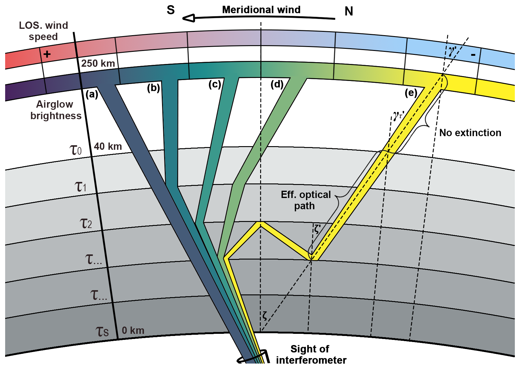
Figure 1 The schematic diagram of the scattering radiative transfer model. The grey shading represents the lower atmospheric layer, with darker hues indicating greater optical depth. The yellow-green fillers represent the relative brightness from the red-line airglow layer. Yellow indicates higher light intensity. The blue-red fillers, which correspond to the relative brightness, represent the Doppler shift type (blue-shift or red-shift) of LOS wind speeds. (a–e) Airglow emissions travelling along different paths, carrying Doppler shifts from outside the line of sight into the interferometer, thereby causing biases in the observations. The model estimates the biases by simulating the distribution of airglow emissions after scattering.

Additionally, the scattering characteristics of the lower atmosphere in our model, including the scattering phase function and optical depth, were derived from Aerosol Robotic Network (AERONET) observations (Holben et al., 2001). We utilized data from the Baotou site (40.9° N, 109.6° E), which is the nearest available site to SIZW, located approximately 180 km away. The total optical depth, accounting for both aerosol and molecular scattering, was calculated using monthly averages and was found to be 0.43 in May and 0.2 in October. The scattering phase function was determined based on AERONET data following the previous method (Harding et al., 2017a). Further details regarding the scattering characteristics are described in Appendix B.

3 Results

Two storms with visible auroras on 10 May and 10 October 2024, respectively, are used to study the scattering impact. The storm from 10 to 11 May is characterized by its significant magnitude and prolonged duration. Multiple works report this event (Guo et al., 2024; Hajra et al., 2024; Themens et al., 2024), with particular focus on the variations of thermospheric winds (Wang et al., 2025; Zhang et al., 2025) and auroras (Gonzalez-Esparza et al., 2024; Kataoka et al., 2024b; Mikhalev, 2024; Nanjo and Shiokawa, 2024) at mid-latitudes. The storm commenced around 17:00 UT on 10 May and the main phase persisted until 02:00 UT on 11 May. After that, the local night of 11 May in the China region sank into a continuous recovery phase. Another storm from 10 to 11 October is weaker than May's (Ranjan and Pallamraju, 2025; Singh et al., 2025), with the main phase from 18:00 UT on 10 October to 02:00 UT on 11 October. During the two geomagnetic storms with visible auroras, both the DCOI and FPI at SIZW observed atypical winds, characterized by intense horizontal wind differences and downward vertical winds.

3.1 Storm-time wind speed statistics

It is necessary to ascertain whether atypical winds originate from atmospheric scattering with spatially uneven airglow brightness or dynamic processes during storms. To investigate the impact of visible auroras on atypical winds during storms, we made the most of the available observations, tracking DCOI's storm-time observations for nearly a year and FPI's for almost five months. We employed the planetary magnetic index Kp (Matzka et al., 2021) exceeding 3 to identify geomagnetic storms (Yang et al., 2020). Besides, to rule out moonlight and cloud effects, we only used clear sky conditions, which means: (1) excluding cases where the angle between the moon and the line of sight is less than 30°, and (2) excluding cases where large-area thick cloud coverage is visible in DCAI. Additionally, data with standard errors greater than 50 m s⁻¹ were also excluded. A few aurora events, including 5 November, 1 December 2023, and 12 August 2024, that did not meet this criterion were excluded.

Figure 2 shows thermospheric wind statistics during geomagnetic storms (Kp > 3) at SIZW. The first two panels display FPI data from May to October 2024, while the rest display DCOI data from November 2023 to October 2024. FPI began operation on 8 May 2024, with about half a year less data than DCOI. Observations with no aurora in the field of view are marked as points, while the two cases with visible auroras are shown as lines. The five observation directions of the interferometer are marked by different colors. During typical storms, horizontal winds consistently increase to around 150 m s⁻¹ both equatorward and westward with no significant downward wind. However, under visible auroras, both DCOI and FPI have detected large wind speeds, such as a southward wind of about 600 m s⁻¹ and downwelling exceeding 100 m s⁻¹. The two series of winds observed along opposite cardinal directions (N-S or E-W) exhibit overt differences, with values exceeding 400 m s⁻¹ and contrary directions. This is markedly different from the wind patterns observed during non-aurora storms, where opposite-direction winds do not show significant divergence. Comparing the results of DCOI and FPI, the observations are largely consistent both with and without auroras. The atypical winds observed simultaneously by two interferometers with different principles suggest a systematic error from outside the instruments. Besides, these simultaneous changes appear in five observation directions, all characterized by enhanced negative LOS speeds, a signature consistent with scattering-induced contamination. Next, the relationship between scattered light and atypical winds will be investigated through simulation.

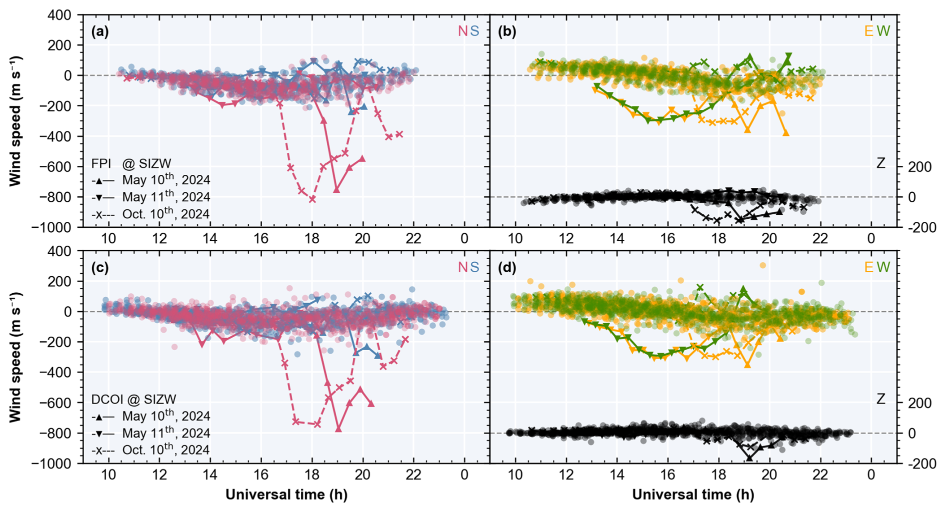
Figure 2 Storm-time (Kp > 3) thermospheric wind speed statistics at SIZW. Panel (a) shows meridional winds observed along two opposite directions (N-S) by FPI, with north-looking in red and south-looking in blue. Panel (b) shows zonal and vertical wind, with east-looking in yellow, west-looking in green, and zenith-ward in black. The northward, eastward, and upward speeds are positive in coordinates. Observations without aurora are shown as points, while those with visible auroras are shown as lines. Panels (c) and (d) are similar but show DCOI data.

3.2 Comparison of observations and simulations

Figure 3 shows the red-line airglow brightness from DCAI (Fig. 3a, e), the observed winds from DCOI and FPI (solid lines with different markers in Fig. 3b–d, f–h) and the simulated winds from the scattering model (dotted lines in Fig. 3b–d, f–h) during the two nights of 10 and 11 May 2024, at SIZW, in which the different colors denote distinct directions. The grey lines in the horizontal wind plots represent the average values between opposite cardinal directions. The multi-directional brightness series from DCAI are extracted at 45° zenith angle, consistent with the scanning zenith angle of interferometers. Time intervals with visible auroras are highlighted in red, showing much higher brightness in northward directions than others. Figure 4 supplements the auroral distribution compared to Fig. 3a and e. Images from DCAI are projected onto the airglow layer at 250 km. The red circle encloses the actual observations with zenith angles less than 70°, while the values outside are extrapolated. The red dots represent the interferometer's pierce points on the airglow layer at 45° zenith angle.

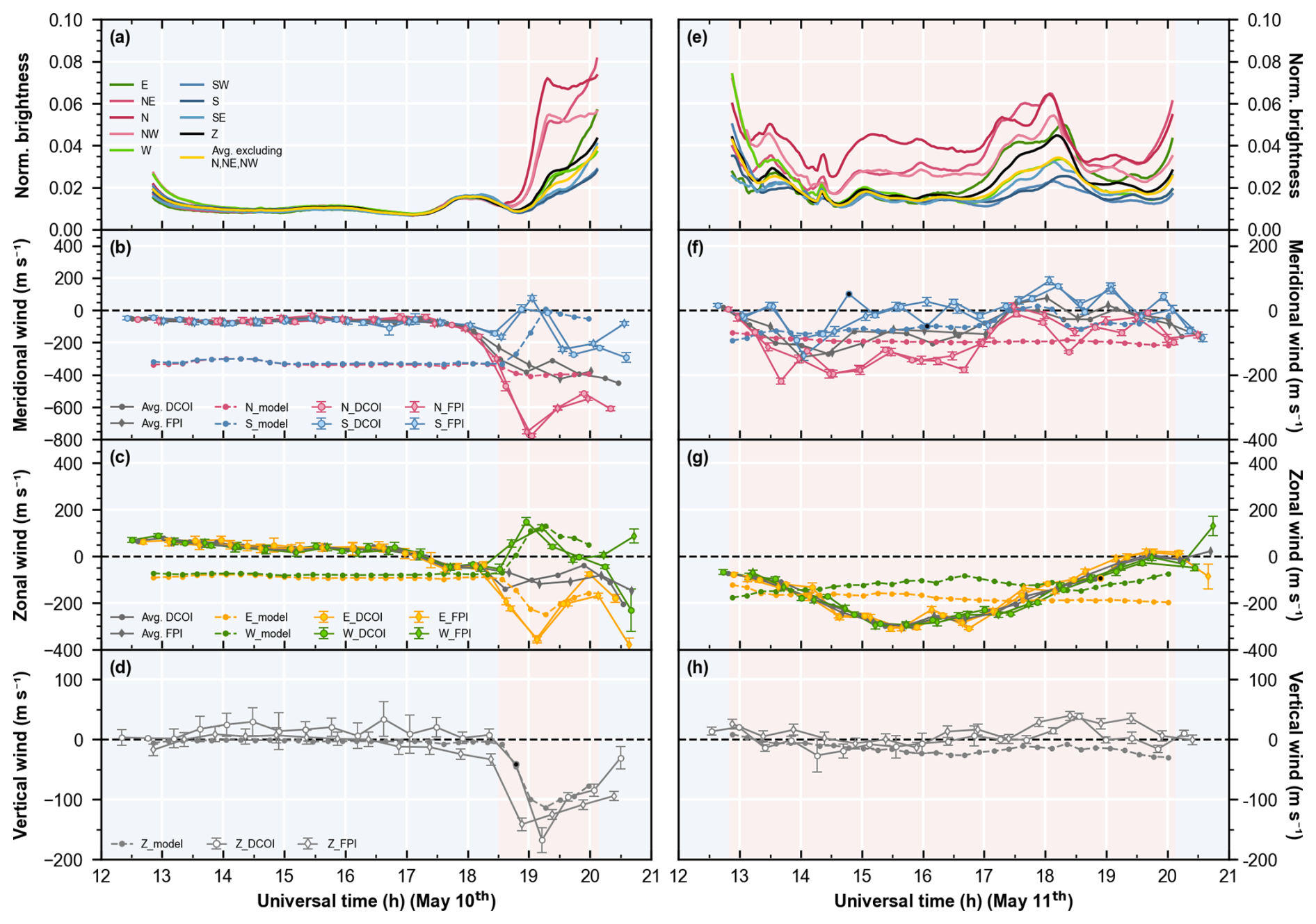
Figure 3 Observations of aurora and wind speeds, and the scattering model simulation on the nights of 10 and 11 May 2024 at SIZW.

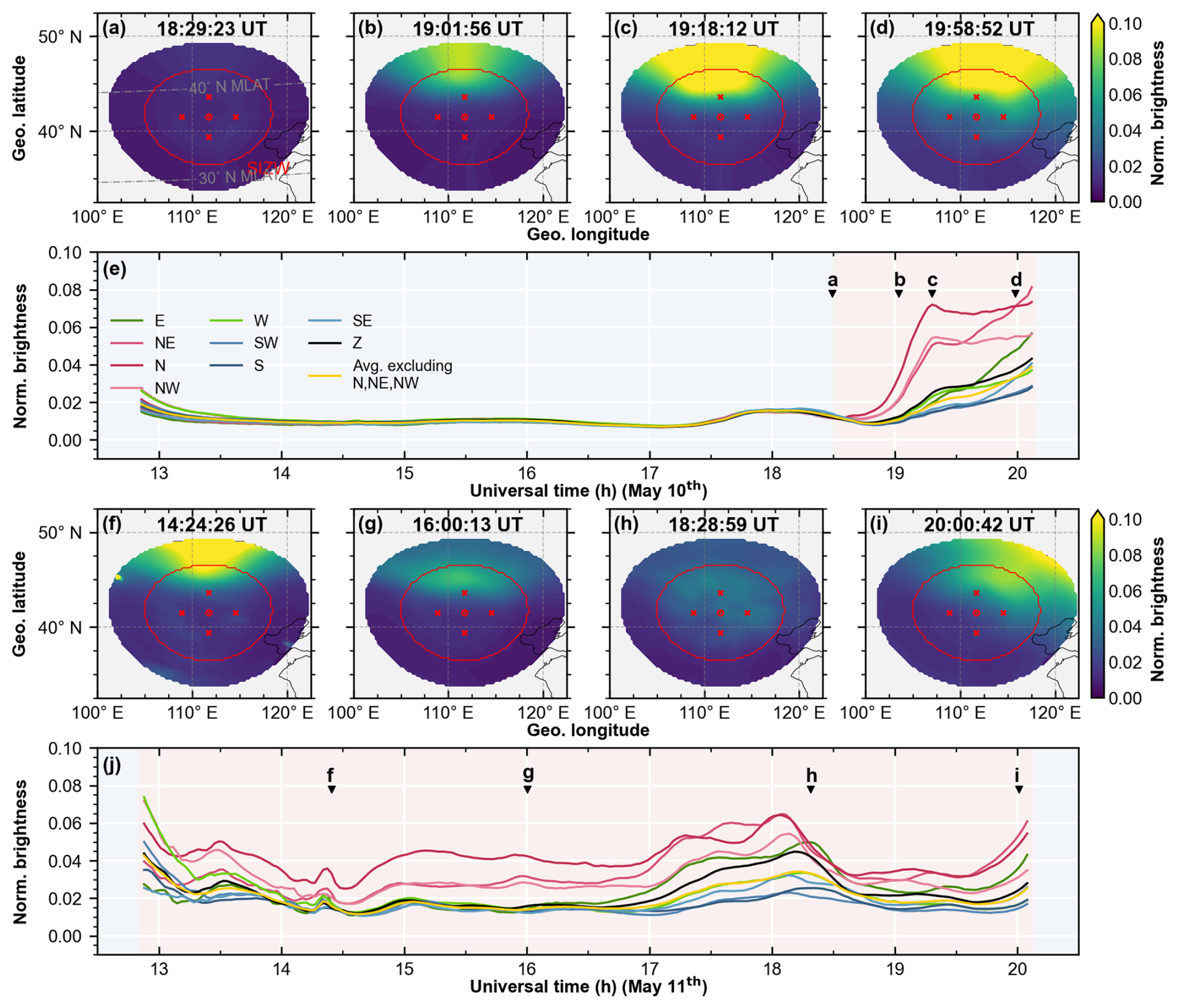
Figure 4 Auroral distribution observed by DCAI on the nights of 10 and 11 May 2024 at SIZW. Images from DCAI (Fig. 4a–d, f–i) have been projected onto the airglow layer at 250 km. The red circle encloses actual observations with zenith angles < 70°, while values outside are extrapolated using zero-order extrapolation. The red dots represent the interferometer's pierce points on the airglow layer at 45° zenith angle. Panels (e) and (j) are similar to Fig. 3a and e, with the corresponding images time labelled. The coastlines in projected DCAI images are made with Natural Earth.

Figure 3a shows the brightness of 8 cardinal directions, all at 45° zenith angle, along with the zenith-ward, extracted from DCAI. The color coding is as follows: red for northern directions, green for east and west, blue for southern directions, black for the zenith, and yellow for the average brightness excluding the three northern directions. Figure 3b shows the meridional wind, with north-looking in red and south-looking in blue, and the average of the two directions in grey. DCOI observations are shown as solid lines with circular dots, FPI as solid lines with rhombus dots, and simulations as dotted lines. Figure 3c and d are similar to Fig. 3b, but for zonal and vertical wind, with east-looking in yellow, west-looking in green, and zenith-ward in black. For a more concise figure, if the standard error exceeds 100 m s⁻¹, the point will be filled with black instead of error bar. Figure 3a–d show data from 10 May and Fig. 3e–h from 10 May. The time intervals with visible auroras are marked in red.

After 18:30 UT on 10 May, as the aurora intensified, both DCOI and FPI detected simultaneous changes in meridional, zonal, and vertical winds. The north-looking red-line brightness at 45° zenith angle exceeded three times that of other directions. The meridional and zonal wind differences between opposite cardinal directions (N-S or E-W) increased. And the winds detected in opposite directions reversed. The maximum meridional difference was close to 800 m s⁻¹, while that in zonal exceeded 500 m s⁻¹. The downward wind was enhanced by over 100 m s⁻¹. These four aforementioned variables that red-line brightness, the meridional and zonal differences, and downwelling, increased almost simultaneously, peaked at 19:05 UT, and then decayed.

Moreover, the average meridional wind, derived from averaging opposite cardinal directions, continuously enhanced equatorward to around 400 m s⁻¹, while the average zonal wind enhanced westward to around 100 m s⁻¹. Unlike the single-direction results that peaked at 19:05 UT, the average wind varied steadily, consistent with storm-time circulation. Compared to the average wind, the separated horizontal and enhanced vertical winds are atypical. Even with travelling atmospheric disturbances (TADs) superimposed on storm-time circulation, phase lags between horizontal and vertical components would be expected (Hernandez and Roble, 1976; Ishii et al., 1999), but none were observed. Thus, the atypical winds do not appear to be the result of a dynamical process. During the recovery phase on 11 May, the aurora was present throughout the night but much weaker than on 10 May, as seen in Fig. 4. Both DCOI and FPI showed westward and equatorward horizontal winds with no significant downward wind. There was a meridional difference of about 100 to 300 m s⁻¹ persisted throughout the night, with no zonal difference.

Subsequently, we used the scattering model to quantitatively examine the relationship between red-line brightness variations and atypical winds through atmospheric scattering. On 10 May, a fixed wind vector of 100 m s⁻¹ westward and 400 m s⁻¹ southward was set as the input. This assumed wind was kept constant over time and spatially uniform, with no vertical components. On 11 May, a fixed wind vector of 200 m s⁻¹ westward and 100 m s⁻¹ southward was used, again with no vertical component. These values are chosen based on average observed wind speeds to approximate storm-time circulation. Although the specific values may deviate, the main wind directions remain consistent. The storm-time enhancement of vertical winds may be caused by scattering rather than representing real winds, so we set it to zero. It is worth noting that we neglect the variation of background wind in the model inputs, due to uncertainty regarding whether the observed wind variations are biased. Moreover, using fixed wind speeds allows us to highlight the impact of red-line brightness variations and determine the presence of scattering effects.

As shown by the dotted lines in Fig. 3b–e, the simulations with scattering impact generally match the observations on 10 May. Assuming a uniform, constant wind field, the scattering model yields horizontal differences (about 400 m s⁻¹) and downwelling (about 100 m s⁻¹) that track the red-line auroral emission, peaking near 19:15 UT before fading. The simulated wind speed variations lag the observations by about 10 min. The lag may be due to the relatively rough 25 min scanning cycle of interferometers or DCAI underestimating airglow brightness at the field of view's edge, leading to inaccurate capture of scattering enhancement start time. Numerically, the simulated zonal and vertical winds match observations more closely than the meridional wind. The simulated meridional difference falls short of the observed value, with the north-looking simulation remaining near the default 400 m s⁻¹ southward while the observation is equatorward-biased at approximately 600 m s⁻¹ southward. The preset fixed wind may influence the meridional simulation, as it does not follow the equatorward enhancement of the meridional wind. Other factors beyond scattering impact might also have an impact, such as the lift of red-line emission profile and the spectral pollution caused by auroras (Makela et al., 2014), to be discussed later. Additionally, the model simulates a similar intense downward wind as observed under the preset zero vertical wind. This indicates that the vertical wind is significantly affected by scattering. This is why the intense vertical wind is not subtracted when converting interferometer LOS speed to horizontal wind, to prevent error propagation. For 11 May, due to the weak but continuous aurora, the simulation shows weak horizontal differences and slight downward winds throughout the night. Compared with the observations, the simulation underestimates the meridional differences by more than 50 %, and it produces zonal differences and downward winds that are not evident in the data. The poorer simulation on 11 May may be due to misalignment between dominant horizontal winds and airglow brightness gradients, which will be discussed later. Additionally, there may be issues with the zero wind calibration. When auroras are present throughout the night, the vertical wind, which includes scattering biases, may have been used to calibrate zero wind speed. It likely masks the scattering impact in the observations and explains the discrepancies in the simulation.

Figures 5 and 6 show another case from 10 to 11 October, analogous to Figs. 3 and 4. On 10 October, the aurora appeared at 17:15 UT, expanded southward and increased in brightness, peaking first at 18:30 UT before decaying and then increasing again from 20:30 UT until sunrise. The second peak was brighter than the first (Fig. 6). Similar to the storm in May, once aurora appeared, both DCOI and FPI observed atypical winds, with synchronous meridional and zonal differences and downward enhancements in vertical wind. These atypical winds also exhibited two peaks, around 18:30 and 21:00 UT. The horizontal winds observed in opposite cardinal directions were basically in opposition. During visible aurora periods, DCOI and FPI showed a 50 to 100 m s⁻¹ difference in vertical wind but consistent variation trends. Moreover, the average horizontal wind between opposite cardinal directions was dominantly equatorward and westward, which also had two peaks. On 11 October, the storm had passed, and no visible aurora was present. The increase in brightness around 13:00 UT was due to moonset in the southwest. There were no significant horizontal differences or downward winds, consistent with geomagnetic quiet conditions.

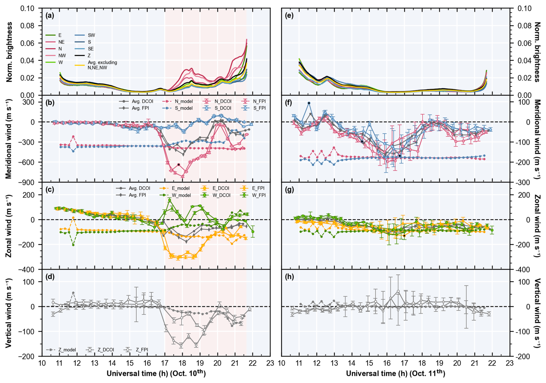
Figure 5 Observations of aurora and wind speeds, and the scattering model simulation on the nights of 10 and 11 October 2024 at SIZW. Figure 5 is analogous to Fig. 3, but for 10 and 11 October.

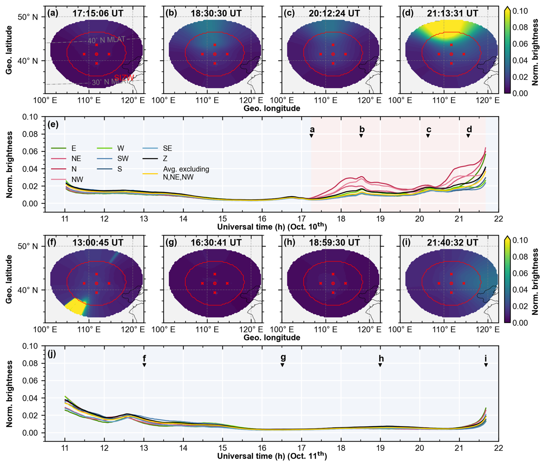
Figure 6 Auroral distribution observed by DCAI on the nights of 10 and 11 October 2024 at SIZW. Figure 6 is analogous to Fig. 4, but for 10 and 11 October.

We set a fixed 100 m s⁻¹ westward with 400 m s⁻¹ southward wind vector for 10 October, and 100 m s⁻¹ westward with 200 m s⁻¹ southward wind vector for 11 October in the model, respectively, with no vertical component. The simulated horizontal wind differences on 10 October also exhibit two peaks. The second simulated peak matches well with the observations, whereas the first peak, though capturing the trend, is underestimated by approximately 75 % of its magnitude. This discrepancy in the simulation may relate to optical depth, aurora brightness, and background wind changes. The optical depth in Oct. is about half that of May, and simulations underestimate observed values. As in previous studies (Harding et al., 2017b), optical depth can affect the scattering model response. On 10 October, the first aurora brightening is weaker than the second. When red-line brightness spatial differences are small, the model response tends to be lower. The impact of optical depth and red-line brightness on the model will be discussed later. Additionally, noticeable fluctuations in the average meridional wind on this day may also contribute to the deviation in the model with fixed initial wind. The north-looking wind speed varied dramatically between 19:00 and 21:00 UT along with the aurora, which may also be related to spectral contamination beyond scattering impact. This spectral contamination arises from fast O atoms generated by low-energy O⁺ ion precipitation in the auroral region, which occurs at higher altitudes. This issue introduces an additional spectral shift that compromises wind retrieval (Makela et al., 2014). This exceeds the simulation range of the model, thereby causing the discrepancy.

4 Discussions

In this study, we modelled the transmission of scattered airglow emission in the lower atmosphere. Post-scattering wind speeds were calculated based on assumed initial wind speeds weighted by both scattered and direct intensities. The model basically captured the temporal variations of horizontal wind differences and downward enhancements associated with varying auroral brightness, suggesting the contribution of scattering mechanisms to atypical winds. However, the simulation of scattering has certain limitations and characteristics: (1) The differences between simulation and observation vary across different directions. (2) The simulated values sometimes exhibit significant numerical deviations from observations. Could this be related to model errors? Next, we will discuss the working principle of the scattering model and the errors involved in the simulation.

4.1 Core working principle of the scattering model

As shown in Figs. 3 and 5, observed winds respond differently to scattering across directions, especially on 10 May and 10 October with stronger auroras. Although the scattering model has numerical errors, the simulations also show directional differences in scattering-induced biases. Both observations and simulations indicate that the meridional wind responds the most, followed by the zonal wind, while the vertical wind responds the least. Since vertical and horizontal wind speeds are derived from the projection of LOS wind speeds, this essentially reflects the non-uniform response of LOS speeds to scattering. This directional inhomogeneity of scattering impact aligns with previous studies. Harding et al. (2017a) simulated scattering effects under auroral conditions, using northward observations as the initial winds. They noted that this direction experiences minimal scattering contamination due to facing the brighter region. Abreu et al. (1983) used a meridional one-dimensional model, finding that LOS wind speeds near intense airglow brightness gradients and with weaker airglow intensity are more susceptible to contamination. They also showed that scattering-induced biases are minimal in the vertical direction, as the shorter atmospheric path length limits the opportunity for scattering. In this study, we further explore the scattering impact as a function of azimuth angle, revealing the formation of horizontal differences.

Figure 7 shows post-scattering LOS speeds at 45° zenith angle in the simulations on three aurora nights, with the vertical axis indicating cardinal directions derived from azimuth angles. Compared with the auroral variations in Figs. 4 and 6, LOS speeds exhibit diffusion during auroras, most evident in Fig. 7a after 18:30 UT on 10 May. Negative LOS speeds initially concentrated to the north, spread westward and eastward, expanding horizontal coverage. Positive LOS speeds initially in the southward direction shrink. When converted to horizontal wind speeds, these changes lead to increased horizontal differences, or the false convergence caused by scattering, in other words. Across all azimuths, the changes of LOS speed share the same sign, but their amplitude scales with the angle to the northward direction. Relative to the roughly 300 m s⁻¹ LOS speed change in the southward direction, the eastward and westward directions each attain about 60 %, whereas the northward variation remains below 10 %. The scattering model shows that LOS speed changes in dimmer airglow regions are more than 10 times those in the brighter zone.

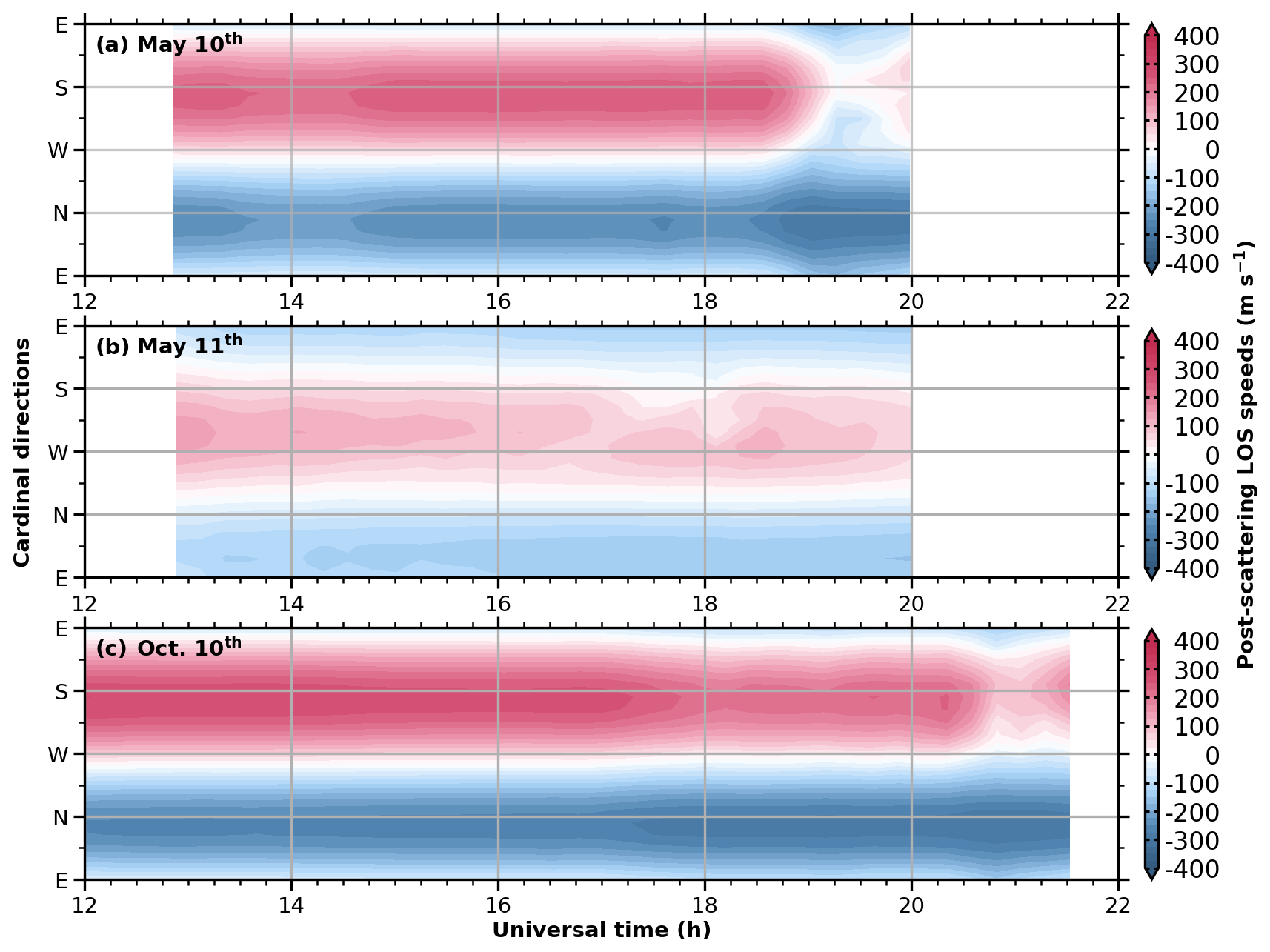
Figure 7 Post-scattering LOS speeds at 45° zenith angle. The figure shows the post-scattering line-of-sight speeds at 45° zenith angle for various directions over time, with panels for 10 and 11 May, and 10 October, respectively.

Figure 8 shows the ratio of scattered light intensity to total light intensity at a fixed 45° zenith angle calculated by the scattering model. Consistent with the schematic diagram (Fig. 1), the scattered intensity is the sum of all injected directions, and the total light intensity includes the direct component on this basis. Without auroras, the scattering proportion is typically below 0.4 and increases with atmospheric scattering capability, rising as the optical depth increases. However, during auroral events, the scattering proportion in some directions can increase to 0.5 or higher. The northward scattering proportion increases the least and remains close to that under uniform airglow conditions. In contrast, the scattering proportion is significantly enhanced in directions ranging from 135 to 180° away from northward. The aurora appears in the north, resulting in much higher northern brightness. After atmospheric scattering, light from the north diffuses into surrounding directions, increasing the scattering proportion. Because the north itself has strong direct light, its scattering proportion remains small. In the model, we assume that stronger light rays dominate interference fringe identification (Wei et al., 2020), thereby determining the Doppler shift or LOS speeds. The lower scattering proportion in the north allows northward observations to retain more LOS speeds from themselves, while other directions experience greater LOS speed contamination from the north. Therefore, as shown in Fig. 7, the northward simulation is closest to the default initial speed, the southward simulation deviates the most, and the eastward and westward simulations lie in between. Additionally, the scattering impact should also consider the initial LOS speeds in the brighter region. Despite the high scattering proportion on 11 May shown in Fig. 7b, the simulated LOS speed changes in Fig. 8b are minimal. This is because of the smaller LOS speed in the auroral region on that day, resulting in less contamination spread to other directions.

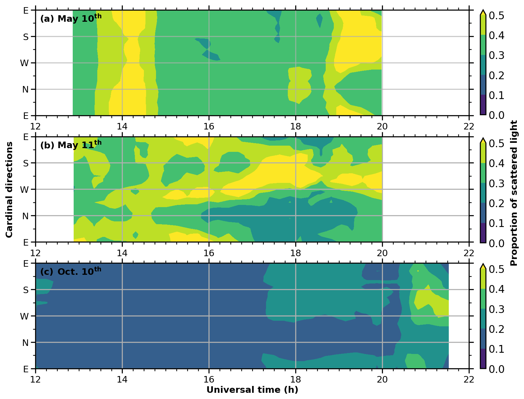
Figure 8 Proportion of scattered light at 45° zenith angle. The proportion is the ratio of scattered light intensity to the total light intensity (both scattered and direct) in the simulation. The figure shows this proportion at 45° zenith angle for various directions over time, with panels for 10 and 11 May, and 10 October, respectively.

The core working principle of the scattering model relies on the relationship between airglow brightness and background LOS wind speeds. As Harding et al. (2017a) noted, scattering requires a bright sky region with large LOS wind speeds. Firstly, spatially uneven airglow brightness is a prerequisite for significant scattering. The brightest airglow area contributes most to scattered light intensity, and its Doppler shifts determine the LOS biases in other directions. This principle allows a rough assessment of scattering impact without model computation when airglow is uneven. Locate the brightest region and its Doppler shift type, as the same Doppler shift type will likely appear in other directions. Blue-shift dominance indicates increased downward wind and horizontal deviations opposite to the line of sight, resembling convergence, while red-shift dominance resembles divergence. Minimal scattering-induced biases occur if the scattering proportion is very low due to uniform airglow brightness, or if the LOS velocity in the bright region is near zero (i.e., the wind speed is perpendicular to the line of sight). Previous observations can be directly verified by this principle and are basically in line with it (Hernandez and Roble, 1976; Price et al., 1995; Ishii et al., 1999, 2001; Makela et al., 2014). Unfortunately, scattering impact can complicate dynamic analysis. In polar regions, auroras are characterized by green-line emissions, and thermospheric winds are significantly influenced by ion drag, where scattering effects may not be prominent. In contrast, mid-latitudes have mainly red-line auroras with large-scale uniform circulation, making the scattering impact more pronounced and distinguishable.

4.2 Errors of the scattering model

The model also exhibits certain errors and limitations. Scattering-induced biases in observations have nearly similar magnitudes on 10 May and 10 October. However, with the same 100 m s⁻¹ westward and 400 m s⁻¹ southward wind input, the scattering-induced biases in the May case are significantly larger in magnitude and closer to reality compared to October. In Fig. 7, the simulated LOS speeds show a larger diffusion range for the 10 May case compared to October. In Fig. 8, the scattering proportion for 10 May is consistently higher than that for October. We attribute this difference mainly to the distinct optical depths in the two months, which are 0.43 and 0.2, respectively. Optical depth reflects atmospheric extinction capability and is mainly related to aerosol content (see Appendix B). It primarily affects the extinction process and influences the magnitude of scattering-induced biases by altering the proportion of scattered light. When the optical depth is artificially raised to 0.5, the model produces a meridional wind difference exceeding 400 m s⁻¹ at 18:30 UT, 10 October, roughly triple the value obtained with an optical depth of 0.2 and in much closer agreement with the observations. We find that the model underestimates scattering effects when the optical depth is low. Once the optical depth reaches 0.6 or higher, the simulated wind bias accelerates nonlinearly until the model diverges.

In the 10 October event, the simulated scattering-induced biases are inconsistent between the two auroral brightness peaks. In Fig. 7, the LOS speed variation is larger during the second peak, and in Fig. 8, the scattering proportion is greater. This is because the scattering proportion is susceptible to errors in scattered and direct light intensities. DCAI does not correct for Rayleigh units, leading to significant errors in regions with large zenith angles. In other words, when the aurora appears at the edge of the field of view, its intensity may be underestimated due to vignetting. It is an effect opposite to the Van Rhijn enhancement. Correcting for Van Rhijn would then further reduce the edge brightness. For now, we extrapolate the edge values of the DCAI imager to mitigate this issue (Appendix B), yet some uncertainty remains. Besides, the model cannot fully eliminate the stray light caused by the glass dome when separating the initial direct and scattered light from DCAI images (Harding et al., 2017a), resulting in errors. In our experiments, if the stray light effect is not subtracted as described in Appendix B, the model becomes more inert, resulting in a smaller simulated scattering proportion. In our experiments, without the stray-light correction in Appendix B, the airglow brightness gradient flattens slightly, the model becomes more inert, and the simulated horizontal wind differences shrink by about 30 %.

We also considered the potential influence of thermospheric temperature. FPI data show uniformly elevated thermospheric temperatures in these two storms, with the northward view occasionally about 300 K warmer than the others (not shown here). Because our scattering model does not yet include temperature effects, we cannot quantify how much scattering biases the FPI temperature measurements. In the study of Harding et al. (2017b), wind simulations are temperature-independent, while temperature retrieval relies on the wind. Likewise, we substitute the LOS speed for the Doppler shift and ignore temperature-induced spectral broadening. In principle, thermospheric temperature influences retrieval uncertainty, not the wind speed itself. We remain cautious that ignoring this uncertainty could introduce extra bias if a horizontal temperature gradient is present, but incorporating it would markedly raise the computational cost and remains a task for the future.

On 10 October, even after the refinements listed below to reduce the underestimation, the scattering model still accounts for only about 25 % of the observed horizontal wind difference: (1) A single-scattering albedo of 1 was used, ignoring absorption. (2) Stray light effects were removed. (3) Attenuated airglow observations at the edge of DCAI images were extrapolated, enhancing edge scattering. (4) Excessive edge extinction was reduced by correcting the extinction path geometry, increasing the scattered light intensity integral. (5) Zero vertical wind was assumed when converting simulated LOS speeds to geographical wind speeds. Raising the optical depth from the observed 0.2 to 0.5 would reduce the underestimation, yet clear-sky DCAI images appear to rule out such high values. We suspect the underestimation arises from how the model integrates the optical depth. Since the integral only includes 10 optical depth layers, with each light ray scattering once per layer and extinguishing once between layers, it may be too crude compared to the real path, underestimating the scattered light. Simply increasing the number of optical depth layers is not effective in our experiments. We think this may be related to the non-linear variation of atmospheric density with altitude, where optical depth may not vary linearly with height, and the scattering phase function may also change with altitude. To address these issues, future work should complete the DCAI correction. Additionally, introducing a model of optical depth varying with altitude can increase the number of single-scattering nodes and ensure the geometric accuracy of the extinction path, thereby improving the accuracy of scattered light intensity calculations.

Furthermore, these bright region observations do not necessarily reflect the usual 250 km thermospheric wind. In Figs. 3 and 5, the north-looking wind observations show unusually high wind speeds, which are significantly different from the simulations. In particular, on 10 October, the north-looking wind speed varied dramatically with the intensity of the northern aurora. During the two auroral peaks, the north-looking wind direction also reversed. This indicates that the interferometer receives an additional effect when it looks toward the aurora. Kataoka et al. (2024b) showed that red aurora lifted the red-line emission profile, raising its peak above 300 km and brightening the upper part on 11 May. Consequently, the interferometer can sample winds that are higher and more poleward. Because storm-time surges propagate from the polar region to the equator, these higher, poleward regions are likely to carry stronger equatorward winds. The interferometer may record a larger wind speed toward the aurora. Additionally, spectral contamination from precipitating energetic ions can also bias interferometers (Makela et al., 2014). In other words, the interferometer is partly sensing the speed of non-neutral species, boosting the observed wind. These issues lie beyond what scattering models can reproduce. From the observed pattern, we infer the presence of non-scattering effects, especially in the poleward view. Due to the absence of nearby higher-latitude neutral-wind observations relative to SIZW, quantifying their respective contributions remains challenging.

5 Conclusions

This study has further proved that lower atmospheric scattering can contribute to biases in thermospheric wind observation on ground-based optical interferometers. During two geomagnetic storms with spatially uneven airglow on 10 May and 10 October 2024, the light scattered from the non-line-of-sight directions of the scope will lead to additional LOS speeds and appear as atypical horizontal differences exceeding 400 m s⁻¹ and downward vertical wind exceeding 100 m s⁻¹ at geographic coordinates. With a simplified scattering radiative transfer model, we simulate the distribution of airglow intensity after the multiple scattering of the lower atmosphere and estimate the wind observation bias under scattering impact via a weighted average method. Starting from the assumed zero vertical wind and spatially uniform, steady horizontal winds (100 m s⁻¹ westward with 400 m s⁻¹ southward), the model produces approximately 400 m s⁻¹ horizontal differences between opposite cardinal directions and 100 m s⁻¹ downwelling on 10 May, in basic agreement with observations, whereas on 10 October it yields only 100 m s⁻¹ horizontal differences, amounting to about 75 % underestimation in magnitude, yet it still captures the temporal trend.

We have refined the scattering model in previous research to enhance its computational efficiency. Specifically, we simplified the LOS wind speed simulation and capped the lower atmosphere at 40 km to refine the extinction-length calculation. The scattering impact can be directly estimated through the relationship between the bright airglow region and the LOS wind speed. The brightest airglow region contributes most to the scattering impact, of which the Doppler shift type determines the LOS biases in other directions. Although the observed winds are affected by scattering when airglow is uneven, they still retain dynamic information, such as the average wind being close to the storm-time circulation. Unfortunately, we lack alternative observational methods to verify the accuracy of the interferometer results. It deserves further study to the extent of scattering impact with more cases and additional instrumental observations. Limited by the accuracy of the model inputs, the scattering model can only simulate the wind features associated with scattering impact under clear sky conditions. It remains incapable of precisely picking out the speed biases induced by scattering impact. Either artificially doubling the optical depth or subtracting stray light can introduce uncertainties exceeding 30 % in simulated scattering-induced biases. Future model improvements could include in situ real-time optical depth measurements, airglow imager corrections, and incorporating vertical optical depth profiles into the model.

Appendix A

In the following appendices, we provide a concise description of the scattering model's operational principles, inputs, and modifications employed in our works. For more detailed solutions, please refer to the article by Harding et al. (2017a).

Based on the radiation transfer theory, Hansen and Travis (1974) and Sobolev (1975) gave the multiple scattering solution. Harding et al. (2017a) extended the initial source function $J_{\mathrm{0}}(\mathit{\tau },u,\mathit{\varphi })$ to airglow surface source, and corrected the missing normalization factor in the scattering phase function (Eqs. A1 to A3):

$$\begin{array}{}\text{(A1)}& {\displaystyle }u{\displaystyle \frac{\mathrm{d}I\left(\mathit{\tau },u,\mathit{\varphi }\right)}{\mathrm{d}\mathit{\tau }}}=-I\left(\mathit{\tau },u,\mathit{\varphi }\right)+J\left(\mathit{\tau },u,\mathit{\varphi }\right)\text{(A2)}& {\displaystyle }\begin{array}{rl}& J\left(\mathit{\tau },u,\mathit{\varphi }\right)\\ & ={\displaystyle \frac{\mathit{\omega }}{\mathrm{4}\mathit{\pi }}}{\int }_{\mathrm{0}}^{\mathrm{2}\mathit{\pi }}{\int }_{-\mathrm{1}}^{\mathrm{1}}P\left(u,u^{\prime },\mathit{\varphi },{\mathit{\varphi }}^{\prime }\right)I\left(\mathit{\tau },u^{\prime },{\mathit{\varphi }}^{\prime }\right)\mathrm{d}{u}^{\prime }\mathrm{d}{\mathit{\varphi }}^{\prime }\\ & +J_{\mathrm{0}}\left(\mathit{\tau },u,\mathit{\varphi }\right)\end{array}\text{(A3)}& {\displaystyle }\begin{array}{rl}{J}_{\mathrm{0}}\left(\mathit{\tau },u,\mathit{\varphi }\right)=& {\displaystyle \frac{\mathit{\omega }}{\mathrm{4}\mathit{\pi }}}{\int }_{\mathrm{0}}^{\mathrm{2}\mathit{\pi }}{\int }_{\mathrm{0}}^{\mathrm{1}}P\left(u,u^{\prime },\mathit{\varphi },{\mathit{\varphi }}^{\prime }\right)\text{sec}\left({\mathit{\gamma }}^{\prime }\right)\\ & f\left(u^{\prime },{\mathit{\varphi }}^{\prime }\right)\exp \left[-\mathit{\tau }L\left(u^{\prime }\right)\right]\mathrm{d}{u}^{\prime }\mathrm{d}{\mathit{\varphi }}^{\prime }\end{array}\text{(A4)}& {\displaystyle }L\left(u\right)=\left[\left(R_{\mathrm{e}}+H_{\mathrm{L}}\right)\cos \left({\mathit{\gamma }}_{\mathit{\tau }}\right)-R_{\mathrm{e}}u\right]H_{\mathrm{L}}^{-\mathrm{1}}\text{(A5)}& {\displaystyle }u=\cos \left(\mathit{\zeta }\right)\end{array}$$

The equations are formulated within an improved local spherical coordinate system, including azimuth ϕ, zenith angle ζ which is represented in cosine form u, and vertical height which is expressed as optical depth τ.

In the case of scattering, as illustrated in Fig. 1, the light intensity along a line of sight, represented by $I(\mathit{\tau },u,\mathit{\varphi })$, consists of two parts, the direct light (Fig. 1a) from the same direction, and the aggregate of scattered light (Fig. 1b–e) from other directions, which is represented by the source function $J(\mathit{\tau },u,\mathit{\varphi })$. Based on the radiative transfer equation (Eq. A1), at each optical depth layer, the scattered light intensity received from all directions will be integrated. Simultaneously, the original intensity in the line of sight will be added to the total scattered light. Besides, the extinction in the path will be calculated according to the optical depth.

There are two potential scattering paths in the lower atmosphere: single scattering (Fig. 1b, c) and multiple scattering (Fig. 1d, e). The model computes them sequentially via an iterative process. In the initial state, there is no light intensity in the lower atmosphere. Therefore, the single scattering will originate solely from the airglow layer, and the source function $J(\mathit{\tau },u,\mathit{\varphi })$ will be equivalent to the initial source function $J_{\mathrm{0}}(\mathit{\tau },u,\mathit{\varphi })$ at this state. By solving Eq. (A1), the model can obtain the single scattered intensity in each direction at every optical depth layer, which is the updated source function $J(\mathit{\tau },u,\mathit{\varphi })$. Then, the multiple scattering can be calculated based on it. Typically, the total scattered intensity will remain relatively constant when accounting for the fourth scattering. By using this iteration, the scattered light and residual direct light in DCAI images can be effectively separated. The residual direct light will subsequently serve as the background intensity distribution for simulating speeds.

In the source function $J(\mathit{\tau },u,\mathit{\varphi })$, the scattering phase function $P\left(u,u^{\prime },\mathit{\varphi },{\mathit{\varphi }}^{\prime }\right)$ quantifies the relative gain of an incident angle to an exit angle during the scattering process. The reference value is based on a unit-radius sphere, which necessitates the introduction of a factor $\frac{\mathrm{1}}{\mathrm{4}\mathit{\pi }}$. Furthermore, ω represents the single-scattering albedo, set as 1. The initial source function $J_{\mathrm{0}}(\mathit{\tau },u,\mathit{\varphi })$ is responsible for introducing the airglow distribution $f(u^{\prime },{\mathit{\varphi }}^{\prime })$. Here, sec(γ^′) represents the secant of the zenith angle at the puncture point of the airglow layer, which helps eliminate the Van Rhijn effect. Additionally, the exponential term with base e is utilized to calculate the equivalent extinction length along an inclined path.

It is primarily the lower atmosphere that significantly scatters and absorbs light (He et al., 2021; Li et al., 2022). Therefore, when computing the extinction length, just employing the cosine of zenith angle u^′ will lead to an overestimation of the effective length, as illustrated on the right side of Fig. 1. To address it, we set an upper boundary H_L of the lower atmosphere at 40 km, assuming an optical depth of zero above this altitude. Using geometric relationships, an equivalent length factor L(u) can be derived, where R_e means Earth radius, and γ_τ represents the zenith angle at the penetration point of 40 km height. This value can be readily calculated by adjusting the target height of the formula for γ. Inside the lower atmosphere, we apply a thin-layer approximation, which also utilizes the geometric relationships at the upper boundary.

$$\begin{array}{}\text{(A6)}& V={\displaystyle \frac{V_{\mathrm{dr}}{I}_{\mathrm{dr}}+{\sum }_k{V}_{\mathrm{sc}}\left(k\right)I_{\mathrm{sc}}\left(k\right)}{I_{\mathrm{dr}}+{\sum }_k{I}_{\mathrm{sc}}\left(k\right)}}\end{array}$$

After working out the background intensity distribution, we partition the LOS speeds at 250 km into several bins. To simplify simulation, the model directly uses LOS speeds corresponding to Doppler shifts. As roughly illustrated in Fig. 1, all LOS speeds are categorized into k = 10 bins valued from highest to lowest, assuming that the LOS speeds within each bin approximate their mean value V_sc. The scattered intensity distribution I_sc is computed by extracting the airglow brightness from the corresponding region of each bin. And, there will be no intensity from other areas during a single bin's computing. According to Eq. (A6), the simulative LOS speed at a specific angle will be an averaged result, where the original speed V_dr is weighted by the direct light intensity I_dr, and the additional speed resulting from scattering V_sc is weighted by the scattered light intensity I_sc. The model directly uses the average within DCOI's 9° field of view as simulated post-scattering LOS speed of interferometers, since DCOI and FPI have not measured the reception gain of light outside their fields of view. We find that due to the coarse model grid, the 9° average is nearly the same as using the nearest single-sight observation. Finally, the LOS speed will be converted to horizontal wind, maintaining the assumption of zero vertical wind to prevent the propagation of scattering biases in the vertical direction.

Appendix B

This appendix details the scattering model's inputs from measurements, supplementing the second section. The background airglow brightness for the model comes from DCAI. Image processing includes: (1) dark field exclusion, (2) median filtering to remove starlight, (3) conversion to the local spherical coordinate, (4) stray light correction, and (5) radial zero-order extrapolation for regions beyond 70° zenith angle. Stray light results from the scattering of strong incident light by the glass dome. During quiet nights without auroras, it is weak and uniformly distributed across all LOS directions. We use the azimuthal average of the nearest quiet night at 45° zenith angle as a reference for weak stray light conditions. After the aurora onset, stray light brightens all directions. The difference between the darkest direction at 45° zenith angle and the reference value is considered the additional stray light caused by the aurora and is subtracted from the entire image. The shown airglow images additionally mitigate the Van Rhijn effect through sec(γ^′) and the atmospheric extinction through $\exp \left[-\mathit{\tau }L\left(u^{\prime }\right)\right]$ (see Appendix A). Since the scattering model already includes these processes, no separate treatment is needed. The optical depth and scattering phase function inputs are shown in Fig. 9. Optical depth is calculated using AERONET's monthly averages, with interpolation at 630 nm. Since only daytime observations are available, local daytime values are used to represent nighttime values. Figure 9a and b show monthly average optical depths at local daytime, with total averages of 0.43 and 0.2. The scattering phase function is a weighted average of molecular and aerosol scattering phase functions from AERONET at 675 nm, which is weighted on the total optical depth of aerosols and molecules.

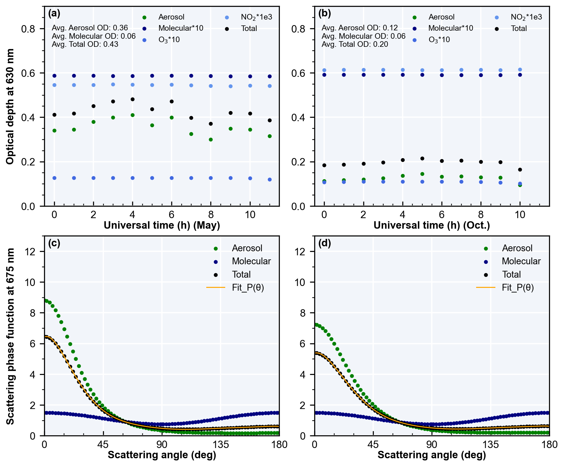
Figure B1 Optical depth and scattering phase function in May and October. The first two panels show daytime monthly average optical depths, with molecular optical depth amplified for clarity. The rest panels show the scattering phase functions.