Laser-Induced Fluorescence coupled with Machine Learning as an effective approach for real-time identification of bacteria in bioaerosols

Microorganisms are ubiquitous in the environment, playing key roles in all ecosystems, including the atmosphere, with airborne dissemination via particulate matter being essential for many microorganisms' life cycles. However, the atmosphere as a microbial ecosystem has been severely understudied, mostly due to the challenging technical difficulties in sampling and characterizing it and the presumed irrelevance of the atmospheric environment for microbes. So far, most recent studies use metagenomic sequencing to assess aerobiome diversity, which can be biased and hurdled due to the inherent ultra-low DNA yield of air samples. Previous research has already demonstrated the potential use of Laser-Induced Fluorescence (LIF) and machine learning (ML) to characterize the vegetal fraction of bioaerosols, by classifying pollen particles using the Rapid-E bioaerosol detector (Plair SA) and neural network classifiers. In this study, we present a new methodology for near real-time (NRT) automatic recognition of microbial particles in the air: first by replacing Rapid-E's visible and ultraviolet (UV) laser (337 nm) with another laser (266 nm) optimized to excite fluorophores in bacterial and fungal cell membranes. We tested this new setup with artificially generated aerosols enriched with five distinct bacterial species. Employing Random Forest classifiers, we were able to: (a) detect bacterial particles (96.74 % class-balanced accuracy), and (b)  discriminate between the different species (69.24 % class-balanced accuracy across the different species in the validation set). This innovative approach sets a new range of possibilities for the rapid and precise monitoring of airborne microbial communities, offering a valuable tool for both ecological studies and public health surveillance.

1 Introduction

Microbial communities are essential components of all ecosystems, contributing significantly to ecological processes and human health. While extensive research has been conducted on the microbiome present in soil (Banerjee and van der Heijden, 2023; Fierer, 2017), water (Cole, 1999), and different surfaces in both urban and rural environments (Gilbert and Stephens, 2018), the atmospheric microbial ecosystem (aerobiome) has remained relatively unexplored until recently (Amato et al., 2023; Tastassa et al., 2024). The atmosphere is a dynamic environment where microorganisms can be transported over long distances (Rodó et al., 2024), influencing both local and global ecological patterns. These airborne microorganisms play crucial roles in nutrient cycling, weather patterns, and even disease transmission (Griffin, 2007; Morris et al., 2011; Fröhlich-Nowoisky et al., 2016; Tellier et al., 2019). Despite their importance, the study of aerobiomes has been hampered by significant technical challenges (Behzad et al., 2015; Luhung et al., 2021a).

Historically, methods for characterizing the airborne microbiome relied on culture-based approaches that missed most microbial species, as most are non-culturable (Eduard et al., 2012). The advent of metagenomic next-generation sequencing (mNGS) revolutionized microbial detection in both clinical and environmental samples, offering culture-independent analysis with higher throughput, faster turnaround times, and greater resolution. However, the ultralow biomass nature of air samples results in extremely low DNA yields (Luhung et al., 2021b). This presents significant challenges for both the qualitative and especially the quantitative characterization of microbial diversity. To accumulate enough material for analysis, the temporal resolution of samples often needs to be compromised (Brodie et al., 2007; Gusareva et al., 2019).

Alternatively, a distinct set of non-invasive fluorescence-based techniques has been developed for the detection, monitoring, and identification of bioaerosols (Crawford et al., 2023). Initially driven by military efforts to detect biological agents (Kwaśny et al., 2023), these technologies have expanded into various civil and scientific fields where timely bioaerosol surveillance is essential. In recent years, several instruments capable of characterizing bioaerosols (primarily focused on pollen) have been commercialized. Notable examples include the Wideband Integrated Bioaerosol Spectrometer (WIBS) series from Droplet Measurement Technologies (USA) (Healy et al., 2014), the KH-3000 from Yamatronics (Japan) (Miki et al., 2021), the BAA500 from Helmut Hund GmbH (Germany) (Oteros et al., 2020), and the Rapid-E series from Plair SA (Switzerland) (Šaulienė et al., 2019; Matavulj et al., 2023). Maya-Manzano et al. conducted a comprehensive comparison and validation of these instruments, among others, for detecting and classifying pollen using Hirst-type traps as a ground truth reference (Maya-Manzano et al., 2023).

While the automation of pollen particle counting and identification is valuable, expanding these capabilities to the microbial fraction of bioaerosols is not trivial. The relatively large size of pollen makes it more suitable for analysis using spectroscopy, especially outside of controlled laboratory conditions. UV-LIF can achieve fine-scale discrimination in the lab, even for small viral particles when paired with machine-learning classifiers (Gabbarini et al., 2019). Translating this capability to real-time, field-deployable systems is challenging because microbial particles in ambient air rarely occur as isolated single particles: they often appear as biological co-aggregates or are embedded within heterogeneous inorganic and organic matrices, both of which complicate both their detection and classification.

In this study, we use the Rapid-E Real-Time Airborne Particle Analyzer, developed by Plair SA (Switzerland), to attempt, to the best of our knowledge, the first methodology to automate the detection and classification of bacterial particles in bioaerosols using a portable device suitable for real-time surveillance in both indoor and outdoor environments.

2 Methods

2.1 Particle Analyzer: Rapid-E

2.1.1 Commercial Device

Rapid-E is the successor to Plair's first particle analyzer, the PA-300, which uses morphological analysis based on scattered light and chemical analysis through UV-LIF (Kiselev et al., 2011, 2013). The instrument is continuously aspirating ambient air and its aerosol particles. Once these are captured, they enter the nozzle, which creates a thin laminar flow in the measurement chamber. Here, two laser beams hit each particle subsequently. First, the particle is hit by a red-light laser beam, whose light gets scattered and detected by 24 detectors positioned at different angles (from 45 to 130°) at a fast acquisition rate and at the same wavelength as the red laser beam.

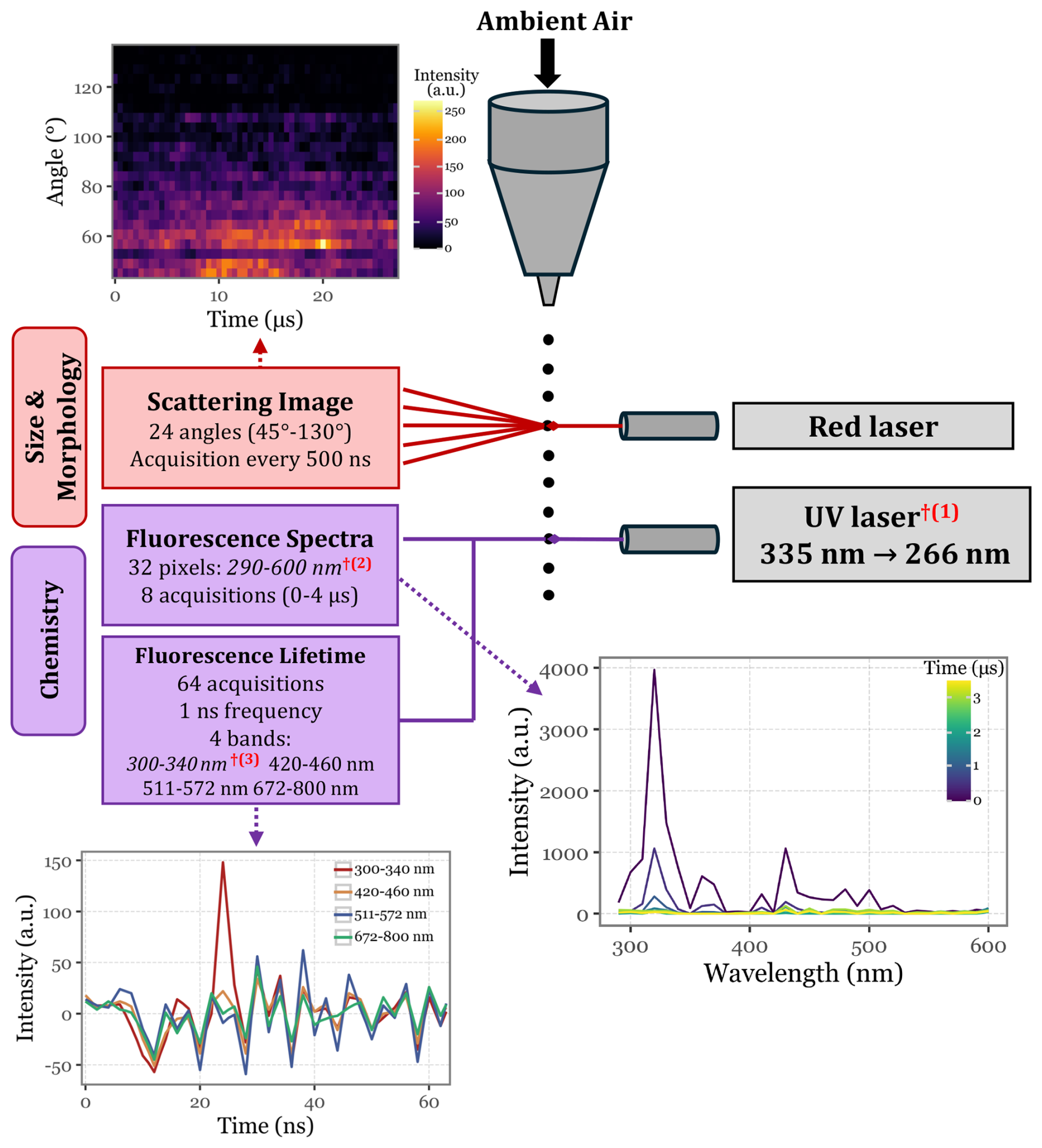
Figure 1 Schematic representation of Rapid-E's operational mechanism, illustrating the data points generated for each particle as it passes through the two integrated laser systems. The red daggers (†) denote modifications made with respect to the commercial version of Rapid-E: (1) the UV laser's excitation wavelength changed from 337 to 266 nm, (2) the fluorescence spectra acquisition range was changed from 350–800 to 290–600 nm, and (3) the first lifetime channel was shifted from 350–400 to 300–340 nm.

The detection of aerosol particles by these detectors generates a trigger signal for the UV laser (337 nm), which in turn hits the particle, exciting its fluorophores. The emission fluorescence spectra (if any) are then acquired by 32 detectors on the spectral range from 350 to 800 nm, and the spectral lifetime is continuously acquired for 4 different spectral bands for a total of 64 ns (at a 1 ns acquisition frequency). See Fig. 1 for a schematic view of the working principle.

2.1.2 Customized Device

For our objective of repurposing the device to focus on the microbial fraction of aerosols, several modifications to the commercially available Rapid-E device configuration were implemented. These adjustments were specifically aimed at adapting to the smaller particle size range of microorganisms compared to pollen, and accounting for the different fluorophore distribution present in microbial cell walls.

The original UV laser integrated into the Rapid-E device operates at a wavelength of 337 nm, selected as a compromise to effectively excite key vegetal fluorophores such as chlorophyll A and B, carotenoids, coenzymes, and various flavins, even though this wavelength does not correspond to the peak absorption of any specific fluorophore. However, to better discriminate the microbial fraction in bioaerosols, it is advantageous to minimize excitation of these plant fluorophores and instead focus on those that are more characteristic of microbial cell walls. These include amino acids (tryptophan, tyrosine, phenylalanine), flavins (riboflavin, FAD, FADH), and coenzymes (NADH, NADPH). These fluorophores typically have excitation peaks at sub-300 nm wavelengths or possess broad excitation spectra that include these shorter wavelengths, generating distinct emission spectra when excited below 300 nm (Pan, 2015). Consequently, we opted to replace the standard laser with a different one with a sub-300 nm primary wavelength.

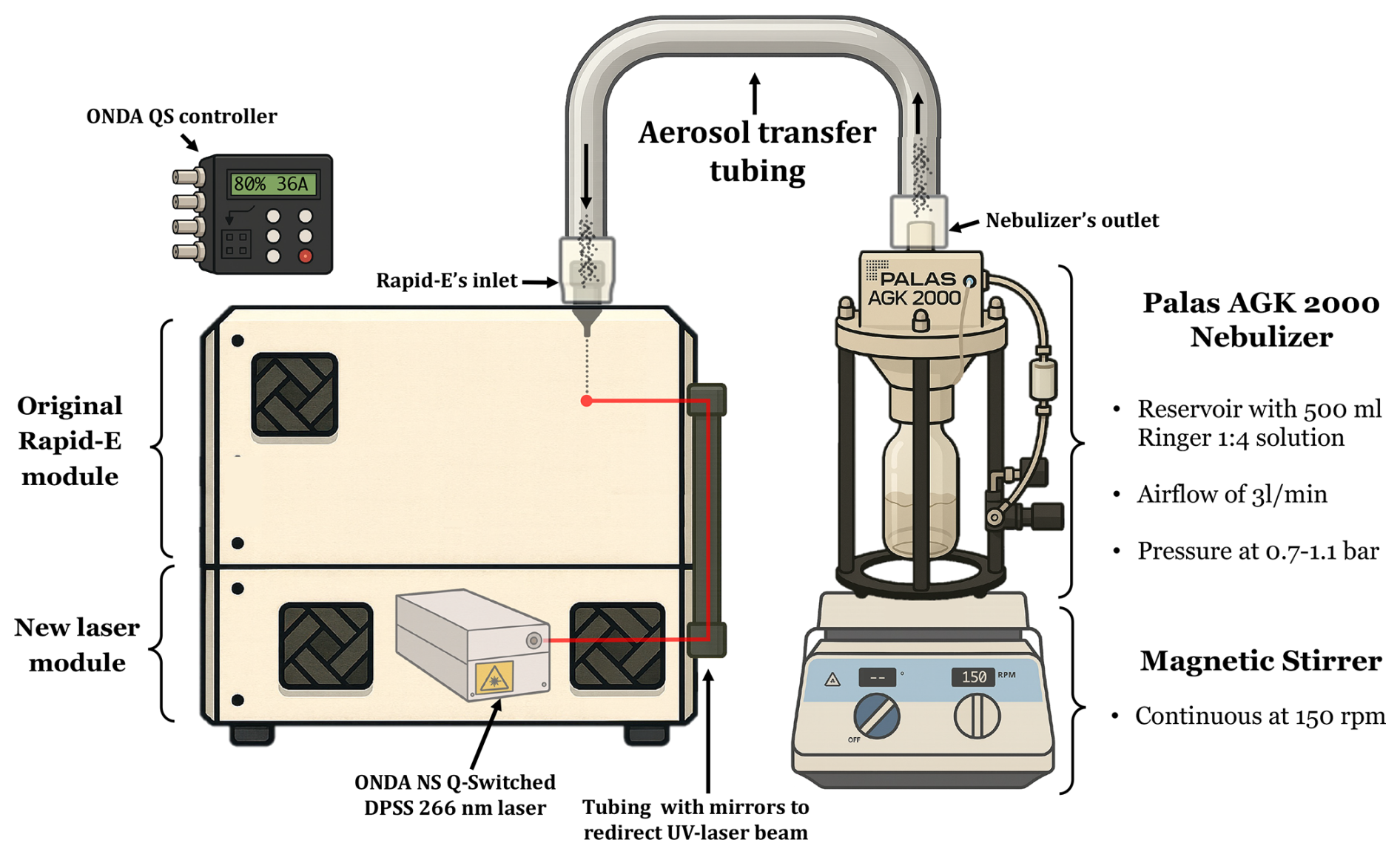
Figure 2 Appearance of the customized Rapid-E device after integrating the new UV laser and its power supply.

The UV laser selected as a replacement was the Onda ns Q-Switched Diode-Pumped Solid State (DPSS) laser (Bright Solutions Srl, Italy), which operates at a primary wavelength of 266 nm, with a maximum peak power of 40 kW, a maximum pulse energy of 80 µJ, and a pulse width ranging from 2 to 6 ns. This laser was integrated directly into the Rapid-E's measurement chamber using mirrors and tubing, along with a new bottom module added to the standard Rapid-E configuration, increasing its height by 15 cm (see Figs. 1 and 2 for the updated configuration). To accommodate the lower excitation wavelength and capture a narrower range of emission spectra, modifications were made to the detectors in both the fluorescence spectra and lifetime modules: the fluorescence spectra acquisition range was adjusted to 290–600 nm (previously 320–770 nm), and the first lifetime module now covers the 300–340 nm range instead of 350–400 nm.

2.2 Experimental set-up

After successfully implementing the modifications into the device, we designed a series of experiments to evaluate:

• 1.

  The feasibility of generating aerosols from solutions and directly introducing them to Rapid-E's inlet.

• 2.

  The effectiveness of the newly integrated laser in detecting and discriminating target fluorophores when aerosolized and isolated.

• 3.

  The device's detection capability when aerosolizing and analysing different isolated and cultured bacterial species.

2.2.1 Aerosolization

We used an AGK 2000 aerosol generator (Palas GmbH, Germany) to generate solid particles from suspensions. In all experiments depicted in the study, we maintained an airflow rate of approximately 3 L min⁻¹ and a pressure between 0.7 and 1.1 bar, with direct connection to the Rapid-E inlet via a sealed, custom-designed stainless steel arm. Solutions to be aerosolized were introduced into the generator's 500 mL reservoir and stirred continuously at low RPM using a magnetic stirrer (Thermo Fisher Scientific, USA) to ensure homogeneity throughout the process.

2.2.2 Fluorophores

We obtained powdered forms of the following molecules, known to be components of bacterial cell walls and exhibiting fluorescent emission when excited at sub-300 nm wavelengths: NADH, riboflavin, tryptophan, and tyrosine (all from Sigma-Aldrich). Solutions were prepared by dissolving 5 mg of each fluorophore in 150 mL of deionized water. For the riboflavin solution, 0.1 M acetic acid was added to a second solution to enhance fluorescence. To ensure the system was free of obstructions, contaminants, or residual particles from previous samples, we aerosolized Milli-Q water for 30 min between each solution.

Table 1 Taxonomic classification of the bacterial species aerosolized in the study.

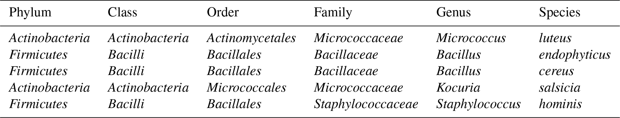
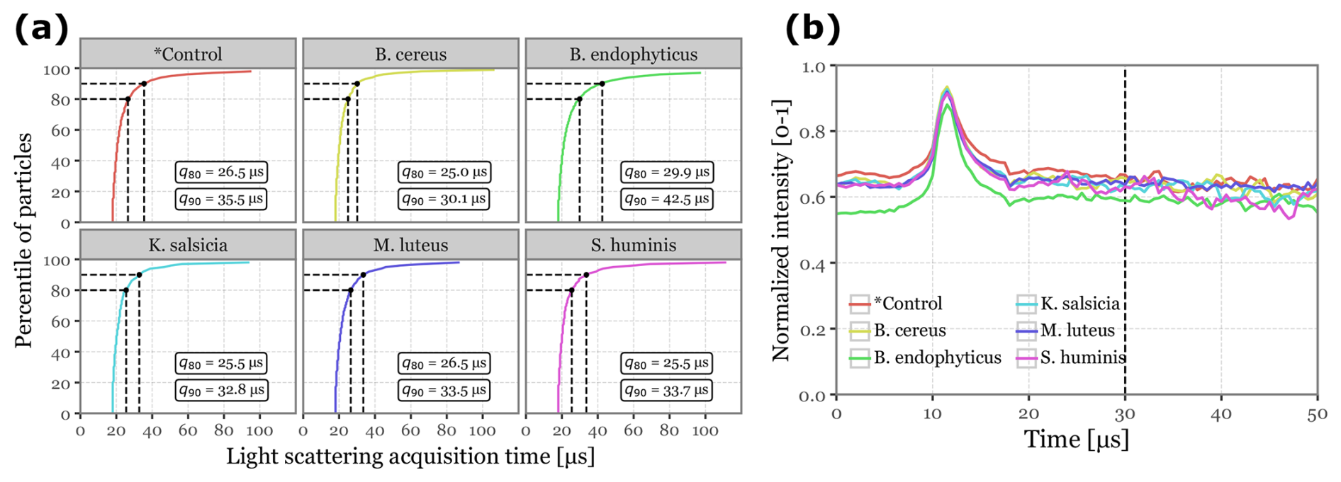
Figure 3 Light scattering intensity acquisition statistics. Panel (a) displays the cumulative distribution functions for the total time of light scattering acquisition per sample for each of the sample groups. Dashed lines and the text boxes indicate the values for the 80th and 90th percentiles. Panel (b) shows the median normalized intensity across all scattering angles as a function of acquisition time for each of the sample groups. The vertical dashed line marks the selected threshold of 30 µs.

2.2.3 Bacteria

We analysed five bacterial species commonly found in urban bioaerosols, which were obtained from air samples collected on quartz fiber filters using a high-volume sampler (MCV, Spain) on the rooftop of our laboratory (AIRLAB, Barcelona, Spain). Filter portions were placed in contact with nutrient agar plates, then removed, and the plates were incubated at 37 °C for 24 h. Morphologically distinct colonies were subsequently subcultured under the same conditions to obtain pure isolates. These isolates were identified using MALDI-TOF MS (LT MicroFLex, Bruker Daltonics, Germany). For each isolate, a small fraction of biomass was spotted onto the target plate, after which 1 µL of a saturated HCCA matrix solution was added and allowed to dry. Each sample was spotted in duplicate, and each spot was measured twice, yielding four mass spectra per isolate. The resulting spectra were compared with the Bruker bacterial library v.9.0. The complete taxonomic classification of the bacterial species used in the experiments is presented in Table 1.

For all the bacteria, a Ringer solution 1:4 was used as the medium, with the negative control consisting of Ringer solution 1:4 alone in the generator's reservoir at the time of aerosolization. Each bacterial isolate was aerosolized for at least 15 min, and to prevent cross-contamination, Milli-Q water was aerosolized for 30 min between each sample. During method development we verified this procedure by tracking minute-by-minute particle counts and the fraction of events above the fluorescence threshold, and confirmed that both dropped to a low, stable background before starting the subsequent sample. Throughout the experiment, the external controller of the Onda ns QS-DPSS laser was set to 80 % (36 A) and Rapid-E was configured in fine dust mode (0.5–100 µm).

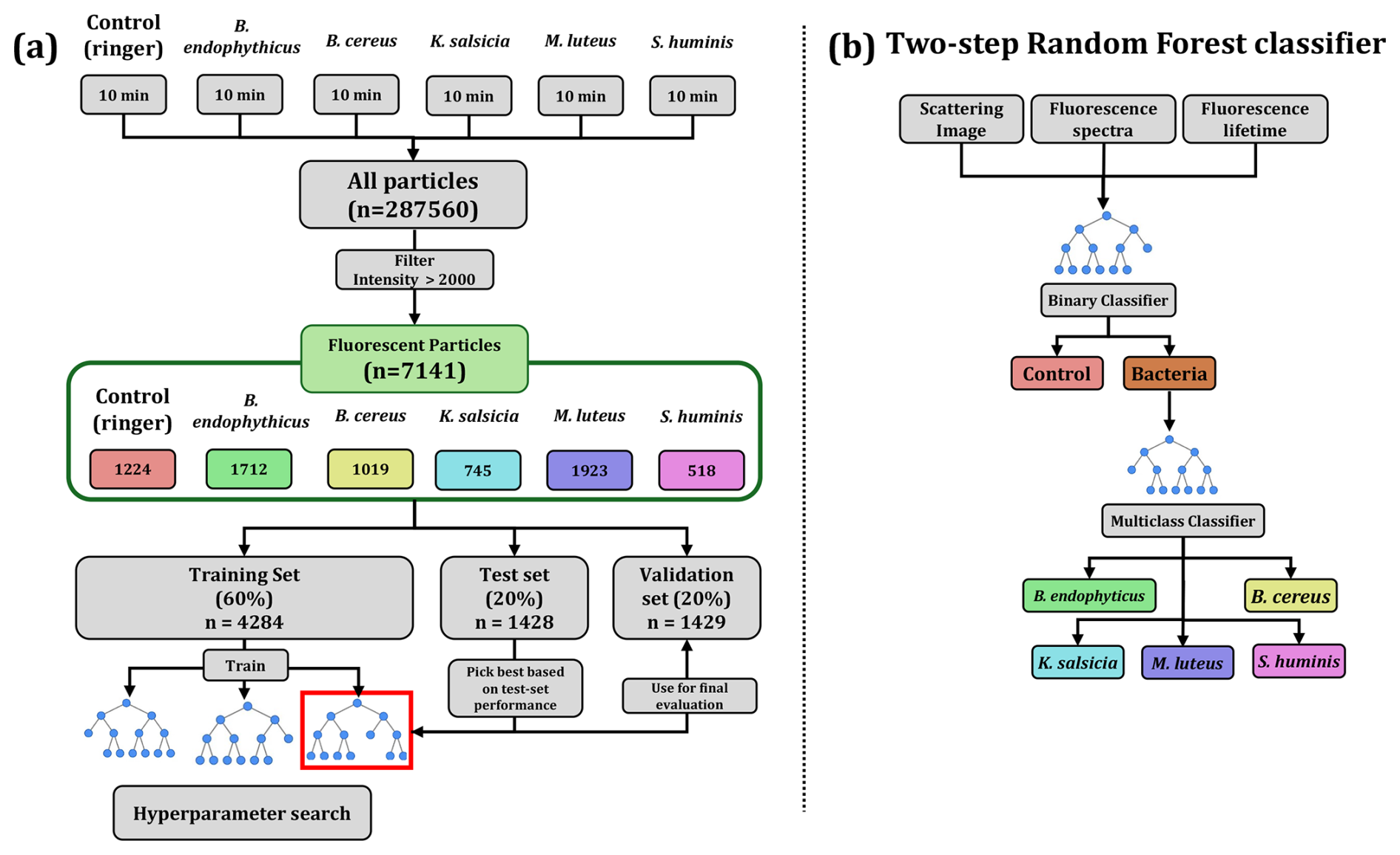
Figure 4 Data flow scheme and model hierarchy. Panel (a) illustrates how the experimental data is handled, filtered and used to train, evaluate and ultimately validate the models. Panel (b) visually describes the two-step approach employed for classifying aerosol particles using random forests: the first step involves a binary classifier to determine whether a particle is bacterial, and the second step employs a multiclass classifier to discriminate between bacterial species if the particle is identified as bacterial by the previous model.

2.3 Data Analysis

2.3.1 Data Processing

After detection, 1 min data files are stored on Rapid-E's internal hard drive. Based on the recorded timeline for each sample, we extracted the last 10 min of aerosolization data for each fluorophore and bacterial sample, ensuring a buffer period between samples to prevent any potential cross-contamination. Given the anticipated irregularity in aerosol particle formation, the uncertainty regarding the proportion of particles containing the targeted biological content, and the need for clear signals to distinguish subtle differences in chemical or morphological composition, we filtered the data to include only particles with recorded peak fluorescence intensities exceeding 2000 $\mathrm{a}.\mathrm{u}.$ at any wavelength and time point. This threshold is higher than the 1500 $\mathrm{a}.\mathrm{u}.$ used by Šaulienė and colleagues for pollen recognition models using the Rapid-E (Šaulienė et al., 2019), as our laser and spectral conditions differ, and we observed significant background noise in peaks below that threshold. In practice, only about 1 %–4 % of detected particles exceeded this threshold. This intentionally biases the dataset toward particles with high signal to noise so that label quality is prioritised over exhaustive sampling of all detected events.

No additional transformation is required for incorporating fluorescence spectra and lifetime data into the models, as these are acquired by the instrument in fixed dimensions (32-channel spectra × 8 acquisitions and 4 lifetime ranges × 64-channels, all later flattened into vectors). However, light scattering images present a challenge due to their irregular shapes, as the total number of acquisitions depends on the duration of the detected scattered light signal. While most particles exhibit signals lasting just 25–30 µs, a significant number required more than 100 µs of scattering signal. Expanding all samples to match the dimensionality of these outliers would drastically increase dimensionality, severely hindering model performance. To address this, we observed that the scattering signal consistently peaked around 10–13 µs across all samples, and that the 80th to 90th percentiles of the total scattering duration fell between 25 and 35 µs. Based on these findings, we cropped the scattering images at 30 µs (equivalent to 60 acquisitions), zero-padded shorter signals, and normalized the values to the [0–1] range. Figure 3 showcases the statistics discussed, along with an example of the final transformed scattering images shown in Fig. S1 in the Supplement.

2.3.2 Random Forest Classifier

For bacterial identification and classification, we trained tree-based machine learning models, specifically Random Forests (Breiman, 2001), to perform two tasks:

• a.

  binary classification to distinguish between control and bacterial samples, and

• b.

  multiclass classification to identify specific bacterial species.

Hyperparameter tuning involved adjusting the number of trees (estimators), the maximum depth of the trees, and the predictors included in the model (all combinations of fluorescence spectra, lifetimes, and scattering images), optimizing for test set accuracy prior to finalizing the model. We split the particles of each group into training, test, and validation sets, representing 60 %, 20 %, and 20 % of the total particles, respectively. The training set was used exclusively for model fitting. In other words, it was the only portion of the data seen by the models. The test set was used to evaluate model performance during hyperparameter tuning, and the validation set was employed for the final model evaluation. A complete diagram of the data flow, model training, and evaluation process is provided in Fig. 4.

Given the class imbalance present in both the binary classification and bacterial species classification tasks, model evaluation was conducted using class-balanced accuracy. This metric was calculated as the average of the recall values for each class (True Positives divided by the sum of True Positives and False Negatives).

To address class imbalance during training, we applied class weight adjustments that were inversely proportional to the frequency of each class. This helped minimize potential bias. The implementation was carried out using the RandomForestClassifier class from the scikit-learn Python library (Pedregosa et al., 2011).

3 Results

3.1 Fluorophores

The aerosolization of fluorophores commonly found in biological particles produced a range of aerosol particles detectable by the Rapid-E device, with varying success rates. The device detected the following particle counts per minute of aerosolization: 4064 for Tyrosine, 3132 for Riboflavin with acetic acid, 2162 for Tryptophan, 1885 for NADH, and 853 for Riboflavin in deionized water.

Regarding fluorescence intensity after the integration of the 266 nm UV laser, most particles did not exhibit sufficient intensity to be classified as fluorescent, with median peak intensities below 800 $\mathrm{a}.\mathrm{u}.$ for all fluorophores. See Fig. 5 for the median, 95th, and 99th percentile values of fluorescence intensity for each class.

Using the fluorescence threshold of 2000 $\mathrm{a}.\mathrm{u}.$, the percentage of fluorescent particles detected was 10.88 % for Riboflavin in acetic acid, 4.9 % for Tryptophan, 2.46 % for Riboflavin in water, 1.59 % for NADH, and 1.03 % for Tyrosine (Fig. 5). These results suggest that metrics focusing on the central part of the particle distribution are likely to be ineffective in distinguishing between groups. Most particles generated in the aerosolization chamber either do not adequately contain the fluorophores or are not effectively excited by the laser, likely due to their small size.

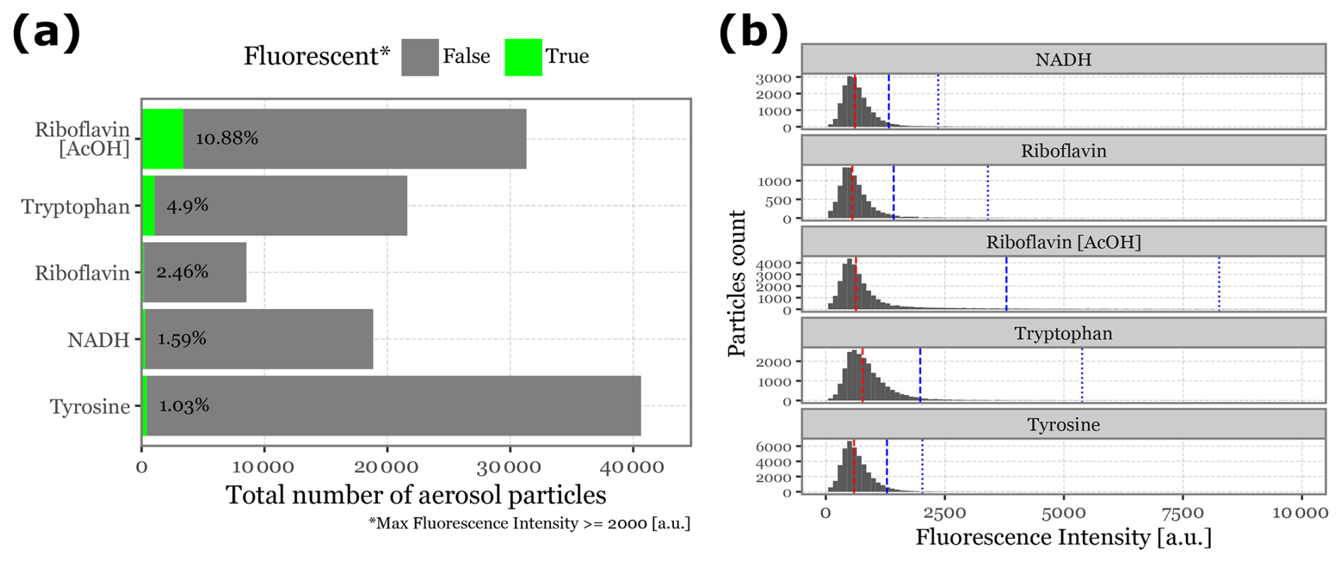
Figure 5 Particle count and fluorescence intensity distribution for biological fluorophores. Panel (a) displays a bar plot showing the total number of aerosol particles generated and detected by Rapid-E over a 10 min period. The green bars (and text) represent the fraction of particles detected as fluorescent, based on a threshold of 2000 $\mathrm{a}.\mathrm{u}.$ for peak intensity at any given time or wavelength. Panel (b) presents histograms illustrating the intensity distribution of all detected particles during the aerosolization of each fluorophore. The red line indicates the median intensity for each group, while the blue dashed line and blue dotted line represent the 95th and 99th percentiles, respectively.

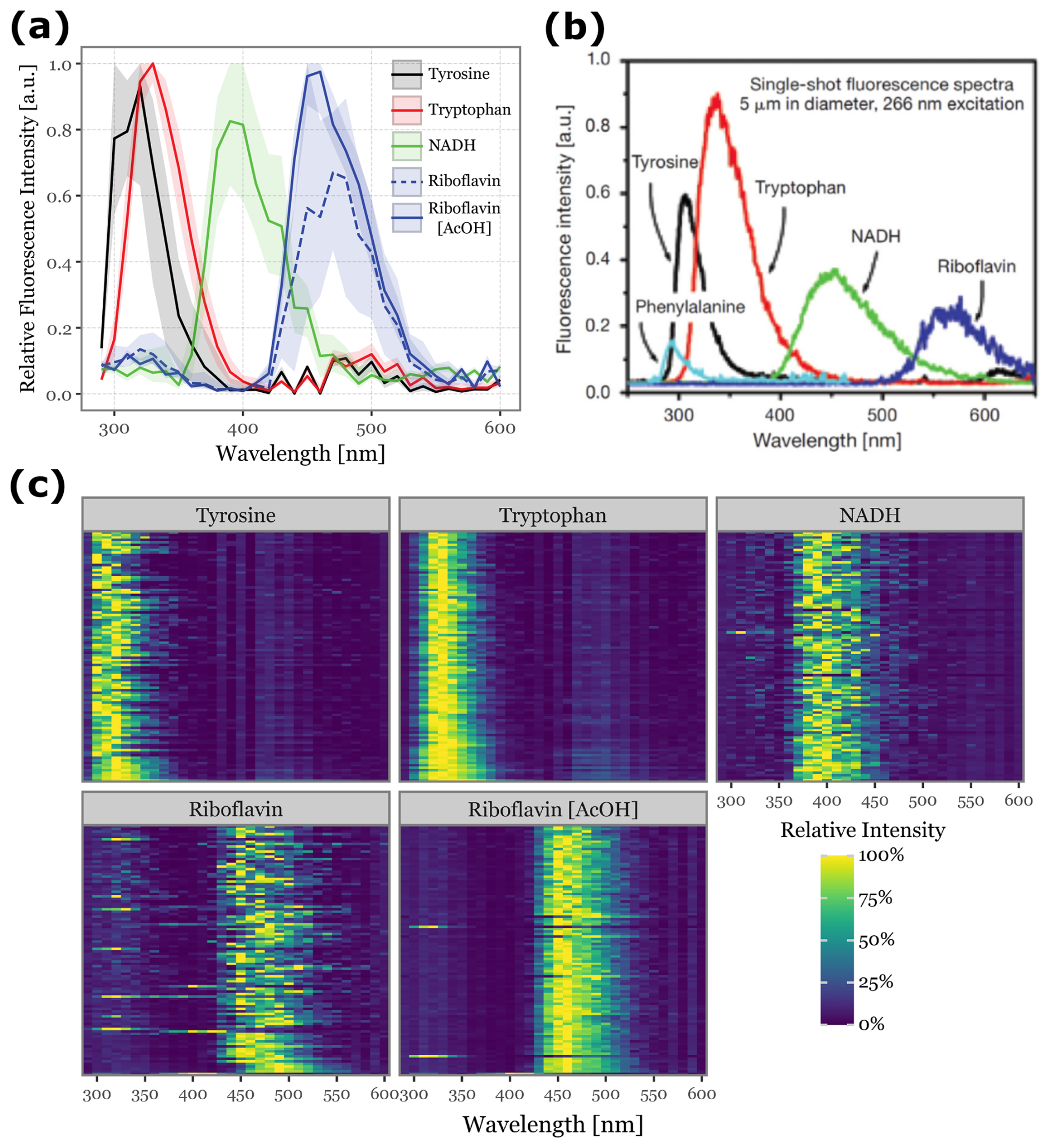
Figure 6 Fluorescence spectra detected for aerosolized biological fluorophores. Panel (a) shows the median fluorescence spectra, aggregated across all acquisitions, for the 100 most fluorescent particles during each fluorophore's sampling period. The shaded areas represent the interquartile range (25th to 75th percentiles). Panel (b) displays single-particle fluorescence spectra excited at 266 nm for common fluorophores found in biological particles, adapted from (Pan, 2015). The colors in Panels (a) and (b) are matched to facilitate comparison. Panel (c) presents a heatmap of the fluorescence spectra for the 100 most fluorescent particles from each fluorophore, ordered from top to bottom.

Fluorescence spectra for the different fluorophores are presented in Fig. 6. To ensure a clean signal, we focused on the top 100 particles with the highest peak fluorescence intensity for each fluorophore. The median spectra and interquartile ranges are shown in Fig. 6a, while the spectra for each of the top 100 particles are displayed in the heatmap in Fig. 6c. Figure 6b provides a reference for the expected fluorescence spectra, adapted from (Pan, 2015), where a single-shot 266 nm laser was used with higher wavelength resolution to excite particles of the same fluorophores at a controlled diameter of 5 µm.

The relative order of the fluorescence peaks we observed (Tyrosine, Tryptophan, NADH, and Riboflavin) aligns with the reference data, validating our results. However, we observed a shift toward lower wavelengths: Tyrosine peaks between 300–320 nm (close to reference values), Tryptophan peaks at 330 nm (compared to 350 nm in the reference), NADH at 390 nm (versus 450 nm), and Riboflavin at 460 nm (versus 550–560 nm). This suggests a potential misalignment in the wavelength calibration of the Rapid-E's fluorescence acquisition system, possibly extending beyond the specified 600 nm range.

The particles with the highest fluorescence intensities also produced the cleanest spectral signals. Riboflavin in acetic acid and Tryptophan exhibited low variability among the samples, in contrast to Tyrosine, NADH, and Riboflavin in water, where sample-to-sample variability was noticeably higher (Fig. 6c).

The fluorescence lifetime values also produced clearly distinguishable signals for all fluorophores, showing fluorescence intensity peaks at around 20 ns after excitation in a single wavelength band for each: Tyrosine and Tryptophan peak in the 300–340 nm band, NADH in the 420–460 nm band, and Riboflavin in the 672–800 nm band (Fig. S4). Again, these values appear to be shifted and do not match the observed fluorescence peaks for the spectra, especially for Riboflavin.

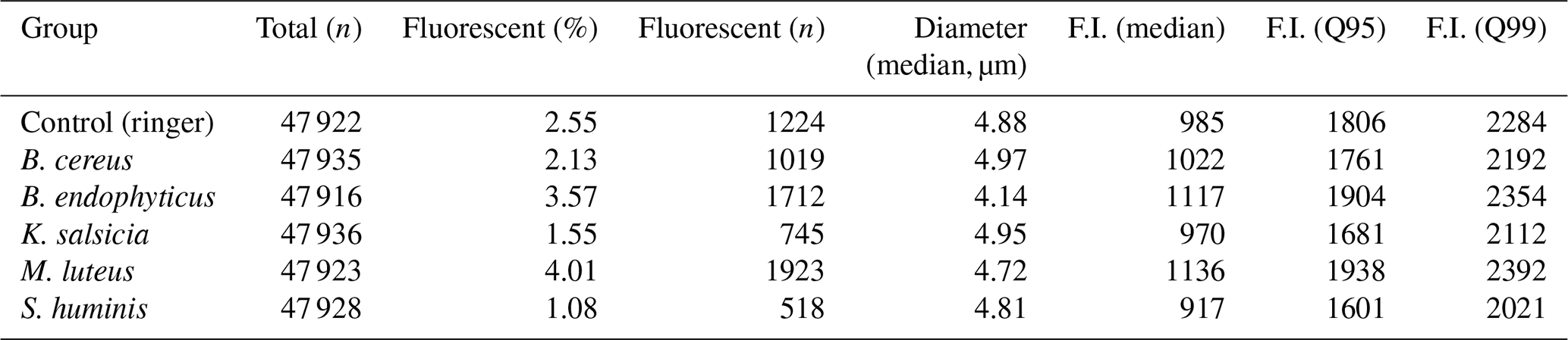
Table 2 Summary statistics for the particles of each of the aerosolized bacterial groups. Fluorescent here implies at least a single reading at any wavelength and acquisition time of at least 2000 $\mathrm{a}.\mathrm{u}.$, and the particle diameters are estimated using the Mie equations based on the scattering images.

These results prove that, while the absolute spectral values may be shifted, the integration of the 266 nm laser successfully generates distinct and recognizable fluorescence spectra and lifetime. Furthermore, the aerosolization protocol produces solid particles consistent enough to be effectively detected by the device, which validates both the laser's performance and the reliability of the particle aerosolization process.

3.2 Aerosolization and descriptive statistics

The aerosolization of the bacterial cultures was successful, generating a substantial number of detectable particles. However, only a small fraction of these particles met the fluorescence threshold of 2000 $\mathrm{a}.\mathrm{u}.$ set for the study. The particle counter of Rapid-E approached near-saturation levels (5000 particles per minute) during the aerosolization of all bacterial samples, including the negative control with Ringer 1:4, resulting in nearly 50 000 particles per group over the 10 min sampling period (see Table 2 for the specific numbers).

Despite this, only 1 %–4 % of the total detected particles exhibited fluorescence above the threshold, leading to a total of 7141 particles included in the final models, with a non-homogeneous distribution: 1923 particles during M. luteus aerosolization, 1712 for B. endophyticus, 1224 for the negative control, 1019 for B. cereus, 745 for K. salsicia, and only 518 for S. huminis. The particle size distributions were consistent across groups, with most particles falling within the 4–5 µm diameter range. Notably, B. endophyticus particles appeared to have a slightly smaller size, ranging from approximately 3.5 to 4.75 µm in diameter (see Table 2 and Fig. S2 for the full distribution).

The signals for the fluorescence spectra, lifetimes, and scattering images were not as distinctly separable across groups as in the pure fluorophore samples, as expected due to the complex biological composition of the bacterial cells and media. This contrasts with the chemically defined bioaerosol samples analyzed in the previous section.

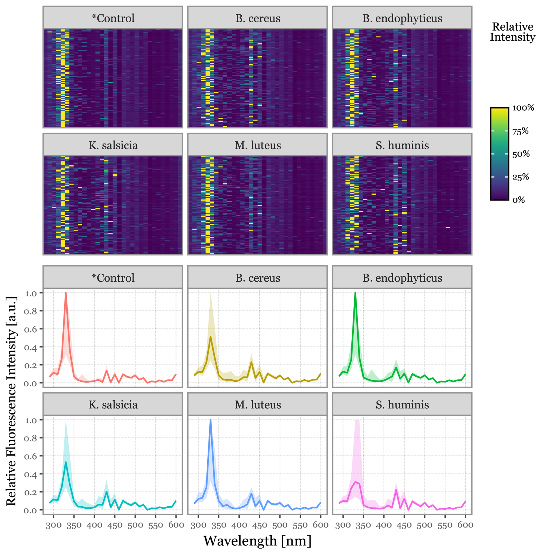
Figure 7 Fluorescence spectra for the aerosolized bacterial samples. In the top panel, heatmaps display the relative fluorescence intensity detected across all wavelengths within the detector's range for the top 100 most intensely fluorescent particles. The bottom panel shows the same data represented as line plots, with the solid line indicating the median value across all samples and the shaded area representing the interquartile range (25th to 75th percentiles).

The fluorescence spectra for each group, as shown in Fig. 7, are presented both for the top 100 most fluorescent particles of each group and as an aggregated distribution of all particles within each category. All groups exhibited a prominent peak around 330 nm, accompanied by a secondary, less pronounced peak in the 400 to 470 nm region. No group-specific spectral features were identified.

The fluorescence lifetimes measured over the 64 ns post-excitation window were notably less intense and exhibited higher noise levels compared to the fluorophores (see Fig. S6 for the bacteria and Fig. S4 for the fluorophores). Nevertheless, the median fluorescence lifetime profiles indicated some variability across groups, particularly in the 300–340 and 511–572 nm bands.

The scattering images (Fig. S5) were largely similar, but some shifts in distribution were observed, particularly in intensity and total signal length. As noted earlier in Fig. 3, B. endophyticus particles demonstrated lower intensity and longer scattering signals.

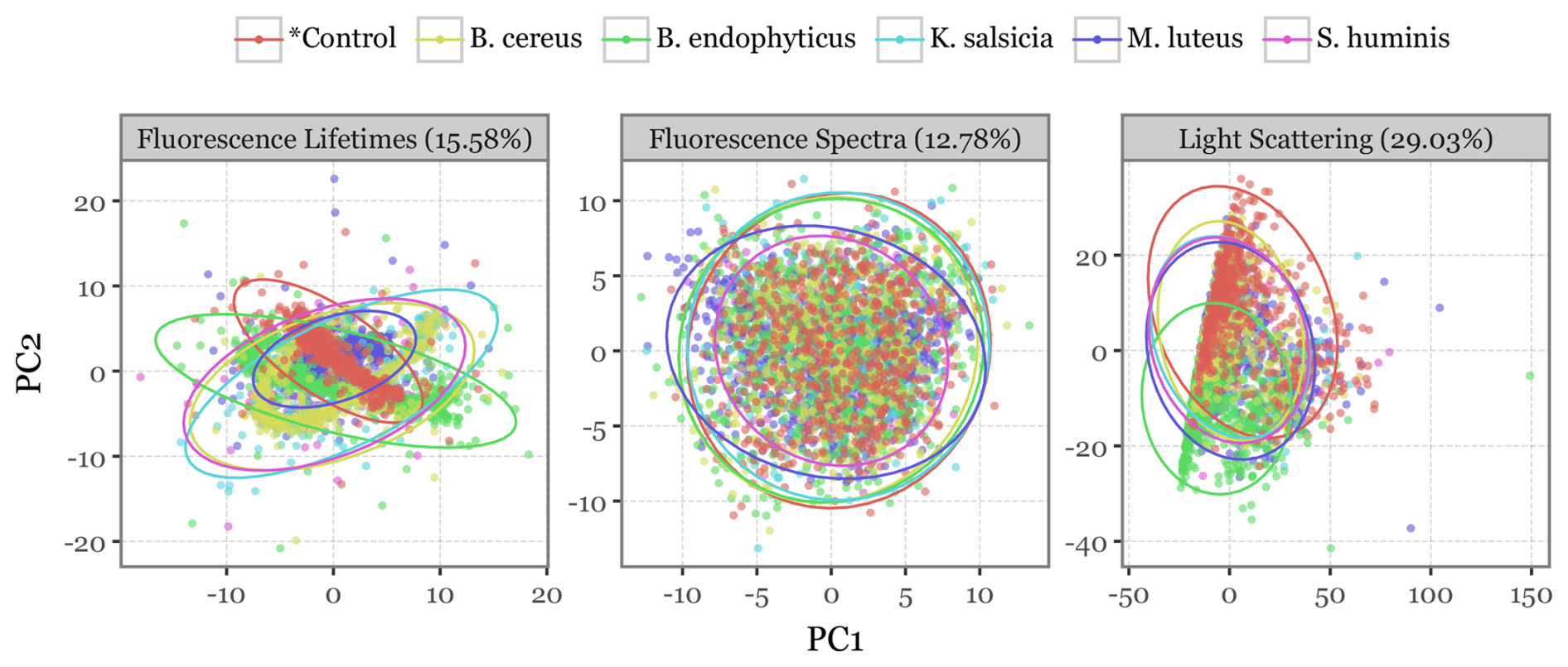
Figure 8 PCA projection of all particles. Scatterplots depicting the first two principal components after a principal components analysis (PCA) decomposition of all variables describing each particle (fluorescence spectra, lifetime, and scattering images) used as input into the models. Colours indicate the bacterial group of each particle, with ellipses representing the 95 % confidence interval of a multivariate t-distribution for the particles in each group. The percentages above indicate the total variance explained by the first two components.

To better visualize the differences among bacterial species, a principal component analysis (PCA) was conducted independently for each of the three data sources, with scatterplots projecting the first two principal components (Fig. 8). The scatterplots show how the bioaerosol particles cluster across groups when projected in two-dimensional space. While all three variables show some degree of overlap among the bacterial groups, the scattering images and especially the fluorescence lifetimes display distinct patterns in the distribution of particles across the first two components, suggesting potentially exploitable differences for classification.

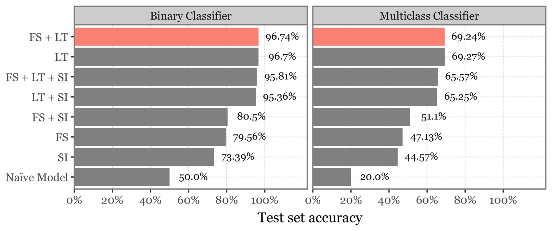
Figure 9 Evaluation of the predictor variables and model skill. Bar plot depicting the class-balanced accuracy of the best-performing model for each combination of model predictors (FS = Fluorescence Spectra, LT = Lifetimes, SI = Scattering Images) for both binary (left) and multiclass (right) classifiers. The bar corresponding to the overall best-performing model, which uses both Fluorescence Spectra and Lifetimes, is highlighted in red. The baseline performance of a naïve classifier, equivalent to a completely uninformed prediction is also included for reference.

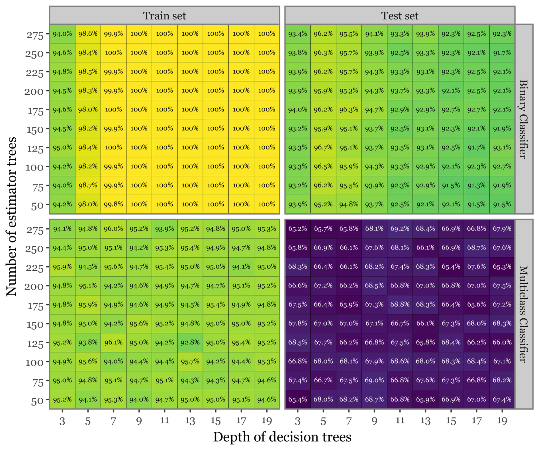
Figure 10 Hyperparameter search and model evaluation summary. Heatmap showing the class-balanced accuracy for both the train and test sets across both model types, focusing solely on the FS + LT models. The squares marked in red indicate the combination of parameters that yielded the best results.

3.3 Model Training and Performance

The performance of the different models during hyperparameter exploration is shown in Figs. 9, 10, and S7. All models, across all combinations of predictor variables and parameter choices, showed a marked improvement over the naïve baseline model in both the binary and multiclass classification tasks. The choice of predictor variables emerged as a key factor, not only contributing to the variance in model performance but also highlighting the critical features necessary for distinguishing between bacterial groups. When evaluating the best-performing models for each combination of predictor variables (Fig. 9), those that included fluorescence lifetimes (FL) achieved the highest balanced accuracy, with 95 %–97 % on the test set for the binary classifier and 65 %–69 % for the multiclass classifier. Conversely, model performance dropped significantly when fluorescence lifetimes were excluded. Models using only fluorescence spectra (FS), and scattering images (SI), achieved a maximum of 73 %–80 % accuracy in the binary classifier and 44 %–51 % in the multiclass classifier.

Models that included both FS and SI, in addition to LT, showed only marginal improvements. The best-performing model achieved 96.74 % accuracy in binary classification and 69.24 % in multiclass classification. This suggests that LT alone captures most of the relevant information.

Fluorescence spectra alone provided a reasonable accuracy of 79.56 % in binary classification but showed a noticeable drop to 47.13 % for multiclass classification. Scattering images were the least effective when used in isolation, achieving 73.39 % in binary classification and 44 %–57 % in multiclass classification.

These observations suggest that while combining multiple predictors can improve accuracy, LT remains the most informative feature for this classification task. The best overall model, selected for evaluation on the validation set, was the FS + LT model. However, this model only marginally improved upon the LT-only model in binary classification (96.74 % vs. 96.7 %) and showed slightly lower performance in multiclass classification (69.24 % vs. 69.27 %).

Figure 10 illustrates the class-balanced accuracies for both the train and test sets across various combinations of the number of estimator trees and the depth of decision trees for the FS + LT model. The results indicate that, while the training set consistently achieved near-perfect accuracy across all parameter combinations, the test set accuracies exhibited a more nuanced pattern. There was a modest decline in performance for the binary classifier and a more pronounced drop (close to 25 percentage points) for the multiclass classification. The highest accuracy for the binary classifier (96.7 %) was achieved with 125 estimator trees and a tree depth of 5, whereas the optimal performance for the multiclass classifier (69.24 %) was observed with 275 estimator trees and a tree depth of 11. The observed disparity in performance between the train and test sets in the multiclass scenario highlights the challenges posed by the high dimensionality of the predictor space. In this context, the model may capture subtle noise patterns rather than genuine signals. This likely explains why a higher number of estimator trees appears to benefit the test set performance by reducing model variance, thereby mitigating overfitting. Despite this, and even if some degree of overfitting is evident, the model still demonstrates strong generalization capability.

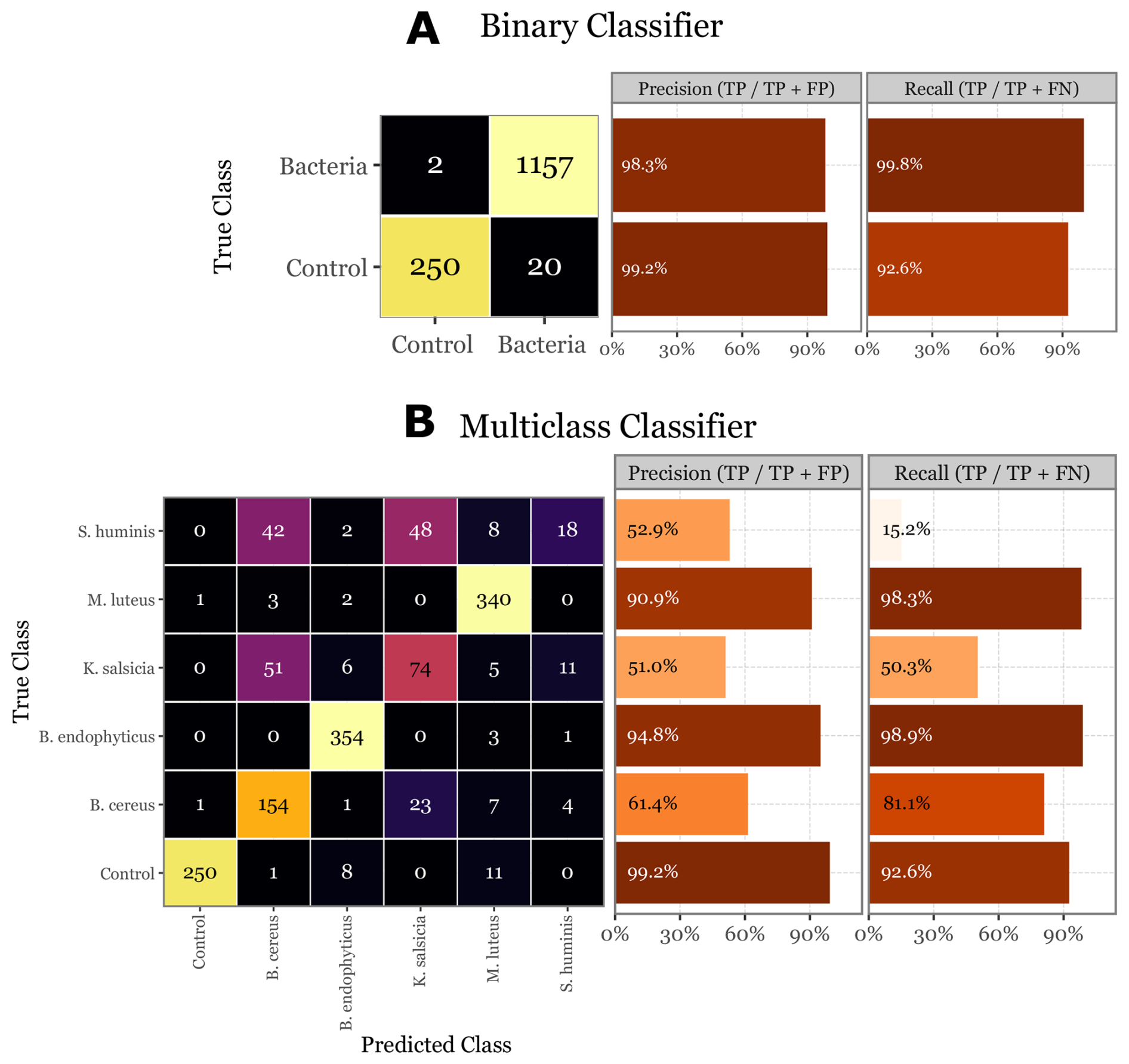
Figure 11 Evaluation of the skill of the Random Forest classifier on the validation set. On (a) the confusion matrix of the validation set for the binary classifier, with the class-specific precision and recall metrics on the right- side bar plots. On (b) the same but for the multi-class classifier. Control class added for comparison and to show the performance on the 20 control samples that the binary classifier predicted as bacteria.

In the final evaluation on the unseen validation set, the binary classifier exhibited strong performance, with a precision of 99.2 % and a recall of 92.6 % for the control class, and a precision of 98.3 % and a recall of 99.8 % for the bacterial class (Fig. 11a). The multiclass classifier, while demonstrating high precision (90.9 % to 99.2 %) and recall (92.6 % to 98.9 %) for certain classes like B. endophyticus and M. luteus, showed significant variability across other classes. Specifically, S. huminis and K. salsicia were less reliably identified, with precision dropping to around 51 %–53 % and recall as low as 15.2 % for S. huminis (Fig. 11b). These worst-performing classes also had lower overall abundance, and despite oversampling them during the training process to compensate, their performance remained suboptimal. This could be attributed to the fact that their lower abundance is due to fewer particles in those groups being fluorescent, indicating that their signals might be less distinct or produce a lower signal-to-noise ratio. Notably, the good performance of both models on the validation set is unbiased and reflects the model's true generalization capability, as the validation set was not used during training or hyperparameter tuning.

4 Discussion

The experimental findings presented in this study highlight a novel application of a Rapid-E bioaerosol analyzer, significantly modified with a 266 nm laser, for the detection and classification of bacterial particles in aerosols. The successful integration of the system is demonstrated by its clear ability to distinguish between isolated fluorophores commonly found in bacterial cells. Crucially, the system effectively differentiates between aerosols enriched with bacteria and control samples, and, remarkably, performs substantially better than baseline models in discriminating between different bacterial species. This enhanced discriminatory power was primarily driven by the inclusion of LT data, which, in conjunction with FS, proved to be the most critical feature set for classification. While our system analyzes individual particles in a flow-through manner rather than providing spatially resolved images akin to Fluorescence Lifetime Imaging Microscopy (FLIM), the fundamental photophysical principles underscoring LT's analytical strength are directly applicable. As extensively documented in FLIM literature, LT is highly sensitive to the fluorophore's microenvironment, largely independent of concentration, and capable of distinguishing spectrally similar species (Berezin and Achilefu, 2010; Datta et al., 2020). Our results, where LT was the most important discriminating feature, align with these principles, suggesting that the temporal decay of fluorescence provides robust signatures for bacterial differentiation. The choice of the 266 nm UV laser was also pivotal, optimizing the excitation of key microbial fluorophores and enabling the generation of these distinct LT and FS profiles. This positions the modified system as a promising tool for real-time bioaerosol monitoring. Despite these promising laboratory outcomes, the transition from controlled settings to complex real-world environmental sampling introduces several challenges that require careful consideration for broader implementation.

On a first note, the contribution of scattering images to the predictive performance of the models seems minimal. Integrating this data into the model failed to improve accuracy and, in some cases, even diminished it. This could indicate that the morphological information contained in the scattering patterns of bioaerosols, despite the system's high-resolution capabilities, does not provide additional discriminatory power for distinguishing bacterial species or for differentiating bacterial from non-bacterial particles when compared to FS and LT data.

Alternatively, this may reflect limitations in our current feature engineering approach or the suitability of random forest classifiers for extracting meaningful features from scattering data. Random forests and tree-based models generally outperform more complex machine learning models such as neural networks when dealing with tabular data (Grinsztajn et al., 2022). However, they may fall short when dealing with complex spatial patterns inherent in scattering images, which bear resemblance to image data. More sophisticated machine learning techniques, such as convolutional neural networks (LeCun and Bengio, 1995), may be better suited for processing this type of data due to their ability to automatically extract spatial hierarchies and features. Previous studies have successfully employed convolutional blocks for feature extraction from scattering images, achieving high accuracy in classifying pollen particles (Šaulienė et al., 2019; Matavulj et al., 2023). However, it is important to note that pollen particles are significantly larger and more morphologically distinct than bacterial cells, potentially making morphological differences more detectable and relevant for classification in those contexts.

Furthermore, the practical deployment of this modified Rapid-E system for extensive environmental campaigns requires consideration of its current physical attributes. As depicted in Fig. 2, the integration of the external 266 nm laser and its associated power supply, along with the additional bottom module, has inevitably increased the overall size and weight of the instrument compared to the commercial Rapid-E version. While the current configuration is well-suited for stationary or semi-stationary monitoring sites where space and power are less constrained, its portability for rapid deployment in diverse or remote field settings could be limited. Future engineering efforts should therefore focus on the miniaturization and more compact integration of these customized components. Achieving a smaller, and lighter design would significantly enhance the system's versatility, making it more readily deployable for a wider range of environmental research campaigns, public health surveillance initiatives, and in scenarios requiring mobile monitoring capabilities. This advancement would be decisive in realizing the full translational potential of the technology for widespread, in-situ bioaerosol analysis.

Beyond bacterial detection, the methodology presented here holds considerable promise for the characterization of other microbial components of bioaerosols, notably airborne fungal spores. Many of the same endogenous fluorophores excited by the 266 nm laser in bacteria, such as tryptophan, NADH, and flavins, are also present in fungal cells (Pöhlker et al., 2012). Furthermore, fungal spores often possess unique cell wall constituents (e.g., chitin, glucans) and pigments (e.g., melanins in dematiaceous fungi) that could contribute to distinct fluorescence lifetime and spectral signatures upon 266 nm excitation. Given that fungal spores are generally larger and often exhibit more complex morphologies than individual bacterial cells, the light scattering data, which showed limited utility for bacterial discrimination in this study, might prove more informative for fungal classification. While the current study focused exclusively on bacteria, the successful application of this modified Rapid-E system and machine learning approach suggests that a similar experimental design could be adapted and evaluated for the real-time detection and differentiation of aerosolized fungi. This would require dedicated studies with diverse fungal species but represents a logical and potentially impactful extension of the current work, further enhancing its utility for comprehensive bioaerosol monitoring.

The observed shifts in fluorescence peak wavelengths for pure fluorophores compared to reference spectra (Pan, 2015), while not impeding relative discrimination in this study, emphasise the importance of instrument-specific characterization and calibration. For broader applicability, such as the development of standardized spectral and lifetime libraries or enabling robust inter-comparison with other devices or techniques, meticulous wavelength and lifetime calibration would be essential. As a practical next step, evaluation of lower-fluorescence isotonic carriers and reduced-salt formulations to further suppress background while preserving cell integrity should be tested given the degree of background noise observed in the time-aggregated spectra.

While the two-step model demonstrated a substantial degree of generalization on our validation set, this capability remains inherently linked to the specific conditions of the training data: artificially generated bioaerosols. Although aerosolizing bacterial samples in Ringer solution 1:4 represents a step towards greater complexity than pure cultures in idealized media, it still falls short of replicating the full heterogeneity of real environmental aerosols. Natural aerosols comprise a dynamic and diverse array of biological (e.g., pollen, fungal spores, plant debris) and non-biological particles (e.g., dust, soot, pollutants), all capable of scattering light and emitting fluorescence to varying degrees (Hill et al., 2001; Després et al., 2012; Pöhlker et al., 2012). In such environments, the spectral, lifetime, and morphological signatures of target bacterial particles may be obscured, mimicked, or altered by other components, leading to potential misclassification or reduced detection sensitivity.

Addressing this will require the development of extensive training datasets that more accurately reflect this real-world variability, a substantial task given the dynamic nature and sheer diversity of environmental aerosols across different locations and times. Two sources of heterogeneity are especially relevant for classification: biological co-aggregates that mix microbial groups within a single event, and inorganic or organic matrices that shift signals through absorption, scattering, and quenching (Savage et al., 2017; Calvo et al., 2018). To mitigate this, in the short term, we suggest an approach with conservative thresholds, permitting unclassified or “bacterial-like” classes when mixtures or strong backgrounds are suspected or model uncertainty is high. Finally, taxonomy is hierarchical, a property that our current model omits, but that means that targets can be structured across ranks with a back-off rule: assign species or genus only when confidence is high, and default to higher ranks when it is not. This is standard practice in sequence-based classifiers such as the RDP naïve Bayesian classifier and MEGAN's lowest-common-ancestor approach, which label to the highest taxonomic rank supported by the data in metagenomics studies (Huson et al., 2007; Wang et al., 2007). The same logic could be adapted here if the class set and evaluation follow the rank structure. Any real usage in the field will need validation with co-located reference sampling to establish site-specific baselines and thresholds.

5 Conclusions

In conclusion, while challenges remain, the results of this study highlight the potential of the Rapid-E particle analyzer, with a UV laser replacement (337 to 266 nm), as a valuable tool for bioaerosol monitoring beyond pollen. With continued research and development, there is a clear pathway toward overcoming the current limitations and realizing the full potential of this technology in diverse real-world applications. The promising results obtained in this study suggest that with further refinement, this approach could become an integral part of environmental monitoring and public health strategies, offering a real-time solution for the detection and identification of airborne bacterial (and potentially fungal) threats. Next research steps should focus on testing realistic particulate matrices that resemble ambient bioaerosols, and on mixtures of bacterial (and fungal) isolates to assess whether composite signatures are consistent and learnable. Meeting these milestones would bridge the technology shown in this study from prototype to robust field deployable tool.