Particulate matter concentrations derived from airborne high spectral resolution lidar measurements using machine learning regression

We use measurements of near-surface aerosol backscatter, extinction, and depolarization acquired by four NASA Langley Research Center airborne High Spectral Resolution Lidars (HSRLs) in machine learning (ML) regression algorithms to derive concentrations of particulate matter (PM) with aerodynamic diameters less than 2.5 µm (PM_2.5), 10 µm (PM₁₀), and the PM_2.5 $/$ PM₁₀ ratio. The ML regression models are trained using airborne HSRL measurements acquired over major metropolitan regions in the United States and Asia that are coincident with hourly surface PM_2.5 and PM₁₀ measurements from the EPA air quality system and similar networks in other countries. We examine several regression methods and find that exponential Gaussian Process regression (GPR) algorithms consistently give the best performance in terms of the lowest root-mean-square (RMS) errors and the highest correlations. When evaluated using surface measurements withheld from the training sets, ML models that use the HSRL near-surface measurements of aerosol backscatter and aerosol intensive properties such as depolarization, backscatter color ratio, and lidar ratio typically give the best performance with RMS differences in PM_2.5 retrievals around 5 µg m⁻³ and correlation coefficients above 0.8, respectively. Corresponding RMS differences and correlation coefficients for PM₁₀ retrievals are 11 µg m⁻³ and 0.7 and corresponding RMS differences and correlation coefficients for PM_2.5 $/$ PM₁₀ are 0.17 and 0.75. This retrieval performance is achieved using airborne HSRL measurements alone and so does not depend on external knowledge of or assumptions regarding aerosol type, aerosol mass extinction efficiency, aerosol hygroscopic growth, the ratio of PM_2.5 to PM₁₀, particle density, or relative humidity. PM_2.5 values in the training set range from about 5 to 80 µg m⁻³; PM₁₀ values range from about 10 to 100 µg m⁻³. Accurate retrievals of PM outside these ranges would require commensurate training data. We present examples of PM retrievals in the United States as well as Asia when HSRL measurements were acquired when the aircraft flew systematic “raster-scan” patterns for several hours over major urban areas. We show that these PM_2.5 retrievals are in good agreement with PM_2.5 derived from coincident airborne in situ measurements near the surface as well as aloft. We describe also how the distribution of PM_2.5 varies with aerosol type and altitude over these regions. We use the HSRL measurements of aerosol extinction and retrievals of surface PM_2.5 along with HSRL retrievals of aerosol type to derive estimates of the fine mode aerosol mass extinction efficiency (MEE_f) for major aerosol types identified by an updated HSRL aerosol classification method. MEE_f ranges from about 2.6 ± 0.5 m² g⁻¹ for maritime aerosol to 5.0 ± 0.7 m² g⁻¹ for smoke. These estimates of MEE_f are also in good agreement with values derived from airborne in situ measurements. We also discuss how this methodology may be applied to measurements from the Atmospheric Lidar (ATLID) on the EarthCARE satellite.

1 Introduction

Aerosol particles, especially particulate matter with aerodynamic diameters less than 2.5 µm (PM_2.5), have been linked to various respiratory and cardiopulmonary diseases and are reported to relate to ∼ 2 to 4 million premature deaths per year globally (Liu et al., 2005; Hoff and Christopher, 2009; Silva et al., 2013; Diao et al., 2019; Strosnider et al., 2019). Smoke from wildfires is of particular concern as recent animal toxicological studies suggest that PM_2.5 from wildfires is more toxic than equal doses from other sources such as ambient pollution (Aguilera et al., 2021; Zhang et al., 2023; Wegesser et al., 2009; Kim et al., 2018). In addition, although PM_2.5 in the USA has decreased over the last few decades, PM_2.5 from wildfires is projected to increase due to climate change (Zhang et al., 2023); in North America climate change contributed to about 15 000 wildfire particulate deaths from 2006–2020 (Law et al., 2025).

Surface PM_2.5 concentrations are monitored by the U.S. Environmental Protection Agency (EPA) and similar agencies in other countries for regulatory purposes. However, the low spatial coverage of these surface stations is problematic for detecting and monitoring PM_2.5 in portions of the United States as well as in foreign countries (e.g., Manila in the Philippines). As an example, since surface stations tend to be in urban areas and far from wildland fires, people living outside the vicinity of an EPA Air Quality System (AQS) monitor (defined by 5 km radius) were subject to 36 % more smoke impact days compared to people living nearby such sensors (Zhang et al., 2023). In addition, surface measurements alone often cannot separate PM_2.5 from fire smoke from other sources (Zhang et al., 2023).

Given the limited coverage of surface measurements, monitoring PM_2.5 from space has been investigated extensively, primarily by using aerosol optical thickness (AOT) derived from spaceborne passive sensor measurements (Chu et al., 2003; Wang and Christopher, 2003; Van Donkelaar et al., 2006; Lee et al., 2012; Xie et al., 2015). These efforts have largely focused on developing correlative relationships between ground-based in situ PM_2.5 (mass per volume) and satellite AOT (unitless, e.g., (Hoff and Christopher, 2009) and references therein). Using AOT measurements from satellites to estimate PM_2.5 takes advantage of the large spatial and temporal coverage provided by spaceborne passive sensors. However, since AOT retrieved from spaceborne satellite sensors is a column integrated property, in regions where AOT variations are associated with aerosols above the surface layer, such as elevated aerosol plumes above the planetary boundary layer (PBL), PM_2.5 (which is a near-surface property) and AOT can be weakly- or un-correlated (e.g., Toth et al., 2014, 2019).

Several studies have used chemical transport models, or CTMs (e.g., Van Donkelaar et al., 2015; Van Donkelaar et al., 2016), to improve correlations between AOT and PM_2.5 and to account for variability in the aerosol vertical distribution. Such models can also specifically simulate PM_2.5 associated with fire smoke thereby enabling epidemiological studies that cover both urban and rural populations. Assimilating satellite AOT data has become increasingly common, significantly enhancing AOT analyses and short-term forecasting (e.g., Zhang et al., 2014; Sessions et al., 2015). However, simulations of PM_2.5 continue to be inadequate (e.g., Reid et al., 2016). Uncertainties in such studies are unavoidable due to uncertainties in the assimilated AOTs and in CTM-based aerosol vertical distributions, as models do not routinely assimilate lidar profiles that can be used for constraining modeled aerosol vertical distributions. In addition, nighttime AOTs are currently unavailable from passive remote sensing satellite retrievals, although efforts are underway to achieve this (e.g., Wang et al., 2023). Attempts to use multisource AOT products (Tang et al., 2019; Liu et al., 2022) or use nighttime light imagery to retrieve nighttime PM_2.5 concentrations are usually limited by moonlight conditions and artificial light sources so that study areas are restricted (Wang et al., 2023).

Lidar measurements can help alleviate these issues. Through their ability to provide the fine scale vertical structure of aerosols as well as by constraining aerosol type (Burton et al., 2012), lidar measurements are very helpful for evaluating and improving models. Ground-based lidars such as those operated in the EARLINET (Pappalardo et al., 2014), ADNET (Sugimoto et al., 2016), and MPLNET (Welton et al., 2018) networks are valuable for providing data for climatological studies, long-range transport events, and model evaluation. Lidar measurements of aerosols at or near the surface avoid uncertainties associated with using column aerosol measurements (i.e., AOT) to infer aerosol concentrations near the surface. Lidar measurements of aerosol extinction near the surface have been used to help derive estimates of surface PM_2.5 concentrations. For example, Li et al. (2017) used an empirical model based on the regression between PM_2.5 and the near-surface backscatter measured by ceilometers to derive surface PM_2.5 at a few selected sites. Coincident ground-based lidar and surface PM_2.5 measurements were also used to derive a linear model to relate aerosol extinction to surface PM_2.5 concentration (Xiang et al., 2020).

Another method, which has been used with space-based Cloud-Aerosol Lidar with Orthogonal Polarization (CALIOP) measurements, uses a bulk-mass-modeling approach whereby PM_2.5 is derived by dividing the CALIOP retrieved near-surface extinction coefficient by the product of the aerosol mass extinction efficiency (MEE) (Hand and Malm, 2007), the scattering enhancement factor [f(RH)] associated with hygroscopic growth of aerosol particles (Hänel, 1976), and the ratio of PM_2.5 to PM₁₀ (Toth et al., 2014, 2019, 2022). Comparisons of surface PM_2.5 derived in this manner with daily-averaged surface measurements of PM_2.5 have shown some success and indicate long-term spatial and temporal variability of PM_2.5 over the USA (Toth et al., 2022). While this methodology generally provides better estimates of PM_2.5 than those derived using only column AOT and PBL heights, such estimates still have relatively large uncertainties and modest correlations due to assumptions regarding these parameters as well as the uncertainty in the near-surface aerosol extinction retrieved from backscatter lidar measurements. These conversion factors typically require some knowledge of the aerosol properties which can vary significantly depending on aerosol type.

Various other methods have used CALIOP measurements to retrieve estimates of PM_2.5. One method used measurements of near-surface aerosol extinction, Aerosol Robotic Network (AERONET) sun photometer retrievals of particle sizes, and assumptions regarding aerosol scattering enhancement factors, particle extinction efficiencies and densities (Ma et al., 2020). Another method has used CALIOP measurements of AOT at various altitude levels, several meteorological variables provided by the Modern-Era Retrospective analysis for Research and Applications, Version 2 (MERRA-2) model, and estimates of the PBL height provided by the ERA-5 model. These data were used with multiple machine learning methods trained using hourly mean PM_2.5 concentrations from surface measurements to estimate PM_2.5 concentrations at the surface and aloft (Chen et al., 2022). This previous study found that the combination of meteorological factors (e.g. air temperature, pressure, relative humidity, wind speed) was more important than layer AOT in retrieving PM_2.5. This result is likely due to the difficulty in using column AOT to infer surface PM_2.5 concentrations as well as the uncertainty in CALIOP retrievals of AOT. In addition, 1064 nm backscatter lidar data from the spaced-based NASA Cloud-Aerosol Transport System (CATS) and the Goddard Earth Observing System (GEOS) model were used to derive surface PM_2.5 (Matus et al., 2025). The CATS lidar data were combined with an ensemble of aerosol profiles from the GEOS Aerosol Data Assimilation System (GAAS). Assimilating the CATS lidar data into the GEOS atmospheric model significantly improved the model's capability to represent the vertical distribution of aerosols.

Elastic backscatter lidars such as CALIOP and CATS have a basic limitation when retrieving AOT and profiles of aerosol extinction. Such lidars measure total attenuated backscatter, which is a combination of backscatter and extinction from higher parts of the profile. Consequently, to derive particulate backscatter, the extinction-to-backscatter ratio, which is also known as the “lidar ratio” (Young, 1995; Omar et al., 2009), must be assumed and/or additional external constraint(s) must be provided. Some methods assume a single, fixed lidar ratio (Xiang et al., 2020) while others, such as that used for CALIOP and CATS, choose fixed lidar ratios that depend on inferences of aerosol type (Omar et al., 2009). Uncertainties in the lidar ratio are the largest source of systematic error in CALIOP retrievals of AOT and aerosol extinction profiles (Winker et al., 2009; Schuster et al., 2012; Rogers et al., 2014). These errors are often largest near the surface, which is particularly problematic for estimating surface PM concentrations. Combining or assimilating the measurements from these lidars with models can help reduce these uncertainties as model simulations of aerosol types can provide estimates of these lidar ratios.

Alternatively, High Spectral Resolution Lidars (HSRLs), such as the airborne HSRL systems from the NASA Langley Research Center (LaRC) and the Atmospheric Lidar (ATLID) on the EarthCARE satellite (Wehr et al., 2023), are particularly valuable because they provide direct measurements of near-surface calibrated aerosol backscatter and aerosol extinction without additional constraints or assumptions to account for attenuation by overlying aerosols. Also, HSRL systems provide measurements of aerosol intensive properties that provide valuable information regarding aerosol type (e.g. smoke, pollution, dust, etc.)(Burton et al., 2012; Groß et al., 2013; Floutsi et al., 2024). During several NASA field missions designed to study air quality, airborne HSRLs have provided profiles of aerosol backscatter, extinction, and depolarization over major metropolitan regions in the United States and Asia. These systems use the HSRL technique to independently retrieve aerosol (and tenuous cloud) extinction and backscatter (Shipley et al., 1983; Grund and Eloranta, 1991; She et al., 1992a) without having to assume the aerosol type or aerosol extinction-to-backscatter ratio. During these missions, these lidars were deployed from aircraft that flew at altitudes ranging from 9 to 13 km and measured profiles below the aircraft thereby providing aerosol profiles near the surface.

LaRC airborne HSRL measurements of aerosol extinction and inferences of aerosol type have been used in an algorithm that associates chemical components with aerosol types inferred from the HSRL measurements to derive estimates of surface PM_2.5 (Meskhidze et al., 2021). In this Creating Aerosol Types from CHemistry (CATCH) algorithm (Dawson et al., 2017), aerosol composition is derived for each HSRL retrieved aerosol type from GEOS-chem model aerosol types based on the aerosol properties measured by the HSRL. The CATCH algorithm links the HSRL inferences of aerosol type with specific aerosol chemical composition and speciation represented by the GEOS-Chem model. The algorithm was applied to airborne data collected over South Korea (Sutherland et al., 2023) as well as several regions in the United States (Sutherland and Meskhidze, 2025; Meskhidze et al., 2021). Comparisons between the derived surface PM_2.5 values and surface measurements from the EPA Air Quality System showed mean absolute errors (MAE) of about 10 µg m⁻³ (Sutherland and Meskhidze, 2025). These results also showed the critical importance of accurate PBL heights in such retrievals since discrepancies in aerosol composition could be attributed to layers of different aerosol types aloft compared to those near the surface; differences in estimates of the PBL height were found to lead to about 20 % variability in the MAE (Sutherland and Meskhidze, 2025). Another approach uses multiwavelength HSRL aerosol measurements in an inversion algorithm to derive aerosol volume concentration profiles; PM_2.5 mass concentration profiles are then estimated by integrating the volume concentration of particles with diameters less than 2.5 µm and applying an assumed aerosol density (Zhou et al., 2025). Initial results showed qualitative agreement with ground station measurements; however, the particle density that must be assumed can vary over a wide range of values and depends on several factors (Pitz et al., 2008; Hasheminassab et al., 2014).

Here we present an alternative method of deriving PM concentrations that uses airborne HSRL measurements in a machine learning (ML) regression algorithm to derive PM_2.5 and PM₁₀ concentrations. Unlike these previous methods (Meskhidze et al., 2021; Sutherland et al., 2023; Sutherland and Meskhidze, 2025) that have used airborne HSRL data to derive surface PM_2.5 concentrations, this method does not require the HSRL qualitative inferences of aerosol type or aerosol chemical composition information provided by models. It also does not require assumptions regarding the aerosol mass scattering and absorption efficiencies, hygroscopic growth factor, the ratio of scattering by fine to coarse mode particles, or particle density. Instead, this new approach takes advantage of machine learning algorithms applied to numerous, detailed, near-surface airborne HSRL measurements of aerosol properties acquired simultaneously with surface PM_2.5 and PM₁₀ measurements; such algorithms have used statistical methods to infer surface PM from lidar (Chu et al., 2013, 2015; Ma et al., 2021) and passive sensors (Fang et al., 2021; Lary et al., 2015; Lee et al., 2021). This approach is somewhat similar to that used to retrieve estimates of cloud condensation nuclei and aerosol absorption using airborne HSRL data (Redemann and Gao, 2024).

We first discuss the airborne HSRL measurements acquired during these field missions. Next, we describe how these data are used in ML regression algorithms to derive surface PM_2.5 and PM₁₀ and show how these retrievals depend on the various aerosol parameters measured by these lidars. We then show examples of these PM retrievals using airborne HSRL data collected during recent NASA field missions. We also discuss the uncertainties in the retrievals and the impacts of the training data on the PM values derived from these regression models. We show how the PM_2.5 varies with aerosol type as derived from a modified aerosol classification algorithm applied to the HSRL aerosol measurements. We then use the retrieved PM_2.5 and PM₁₀ values in conjunction with the HSRL measurements of aerosol extinction to derive estimates of fine mode mass extinction efficiency for these aerosol types. Finally, we discuss the potential use of these machine learning regression techniques for retrieving PM_2.5 from satellite lidars such as the ATLID instrument on EarthCARE (Wehr et al., 2023).

2 Methodology

2.1 Airborne HSRL Measurements

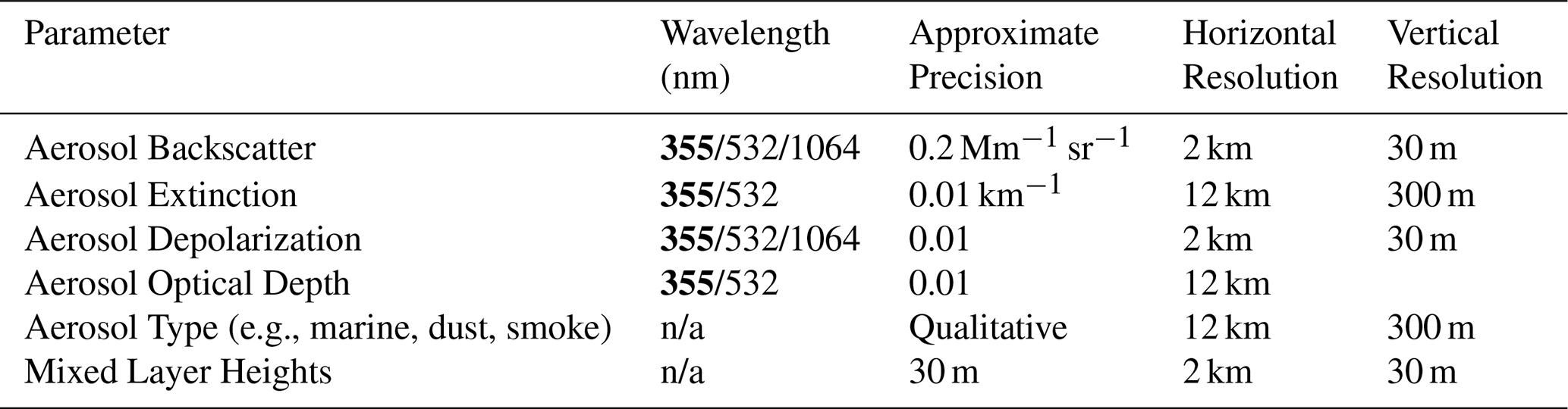
Our methodology takes advantage of a unique set of airborne HSRL measurements acquired by four airborne HSRL systems developed at NASA Langley Research Center. These lidars include HSRL-1 (Hair et al., 2008), HSRL-2 (Burton et al., 2018; Ferrare et al., 2023), DIAL/HSRL (Browell, 1989; Hair et al., 2008), and HALO (Carroll et al., 2022; Barton-Grimley et al., 2022). Each of the airborne lidars employs the HSRL technique at 532 nm to independently retrieve both aerosol extinction and backscatter (Grund and Eloranta, 1991; She et al., 1992b; Shipley et al., 1983) without a priori assumptions regarding aerosol type or extinction-to-backscatter ratio. The HSRL technique measures both total attenuated backscatter and attenuated molecular backscatter which are used to directly derive both aerosol extinction and backscatter and consequently the lidar ratio. The ability of HSRL to independently measure extinction and backscatter is a huge advantage over standard backscatter lidars. By measuring the ratio of the total (molecular + particulate) to the molecular signal, the HSRL technique permits measurements of calibrated, unattenuated aerosol backscatter. The vertical derivative of the attenuated molecular backscatter signal measured by HSRL provides the aerosol extinction profile (Hair et al., 2008). HSRL-2 also uses the HSRL technique to measure aerosol backscatter and extinction at 355 nm. These lidars employ the standard elastic backscatter lidar technique to measure aerosol backscatter at 1064 nm. All these lidars measure particulate depolarization at 532 and 1064 nm; HSRL-2 also measures particulate backscatter, extinction, and depolarization at 355 nm. Aerosol and cloud measurement parameters for these lidars are summarized in Table 1.

Table 1 Measurement parameters, wavelengths, resolutions, and precision for aerosol products measured in the nadir direction by the airborne HSRL systems discussed in the text. Horizontal resolutions are based on aircraft flying at approximately 200 m s⁻¹. All the airborne HSRL systems measure the parameters at the wavelengths shown in black; the additional parameters measured by HSRL-2 at 355 nm are shown in bold.

Additional products are derived from the aerosol profiles measured by these lidars. Backscatter color ratios and Angstrom exponents are derived from the ratio of aerosol backscatter at two wavelengths; spectral depolarization ratios are similarly derived from the ratio of particulate depolarization at two wavelengths. The lidar ratio is also derived from these measurements. Mixed layer heights (MLHs), which are often associated with sharp gradients in aerosol backscatter profiles, are also derived from these data; these heights have been found to be in good agreement with boundary layer heights (BLHs) derived from radiosondes (Scarino et al., 2014). Aerosol type is derived using a classification algorithm to interpret the information about aerosol physical properties indicated by the measured aerosol intensive parameters¹ (Burton et al., 2012).

A significant advantage of the HSRL technique is that it does not rely on apportioning part of the measurement profile for calibration (Hair et al., 2008) unlike standard elastic backscatter lidars that must assume negligible aerosol in a calibration region. As described in detail by Hair et al. (2008), through careful system design and operations, the channel gain ratios and filter transmission are accurately measured to enable this self-calibration. All the depolarization channels and the aerosol and molecular measurements at 532 nm are self-calibrating, while the 1064 nm backscatter and the 355 nm HSRL-2 measurements take advantage of the calibrated HSRL measurement at 532 nm. The overall systematic error associated with the backscatter and depolarization calibration is estimated to be less than 2 %–3 %. Under typical conditions, the total systematic error for extinction is estimated to be less than 0.01 km⁻¹ at 532 nm. The random errors for all aerosol products are typically less than 10 % for the backscatter and depolarization ratios (Hair et al., 2008). A study designed to validate the HSRL extinction coefficient profiles (Rogers et al., 2009) found that the HSRL extinction profiles are within the typical state-of-the-art systematic error at visible wavelengths (Schmid et al., 2006). Column AOT values derived from HSRL-2 data were found to be in excellent agreement with coincident measurements from AERONET (e.g. Sawamura et al., 2017). LaRC airborne HSRL measurements have been used to assess WRF-Chem regional model representations of aerosol backscatter and extinction profiles (Fast et al., 2011, 2014; Saide et al., 2022) as well as evaluate operational (Rogers et al., 2011) and advanced research-type (Burton et al., 2010; McPherson et al., 2010; Josset et al., 2011) CALIOP aerosol profiles, advanced Moderate Resolution Imaging Spectroradiometer (MODIS) retrievals of AOT (Munchak et al., 2013), extinction profiles derived from airborne in situ measurements (Ziemba et al., 2013), and AOT derived from other remote sensors (Kassianov et al., 2010; Knobelspiesse et al., 2011; Shinozuka et al., 2013).

2.2 Airborne HSRL Data Sets

The airborne HSRL systems discussed above have acquired data over several major cities in the United States including Washington D.C., Baltimore, Houston, Los Angeles, Chicago, and New York City, as well as major cities in Asia including Seoul (South Korea), Manila (Philippines), Tainan-Kaohsiung (Taiwan), and Bangkok (Thailand) during several NASA field missions conducted since 2010 as shown in Fig. 1. These HSRL measurements were often acquired when the aircraft flew systematic “raster-scan” patterns for several hours and often repeated multiple times per day. These flight patterns provided the opportunity for the airborne HSRL to observe the spatial and temporal variabilities in distributions of aerosol backscatter, aerosol extinction, and AOT over these cities. For the missions considered in the study, the HSRL systems were deployed from several different aircraft including the NASA King Air B200, G-III, G-V, and DC-8.

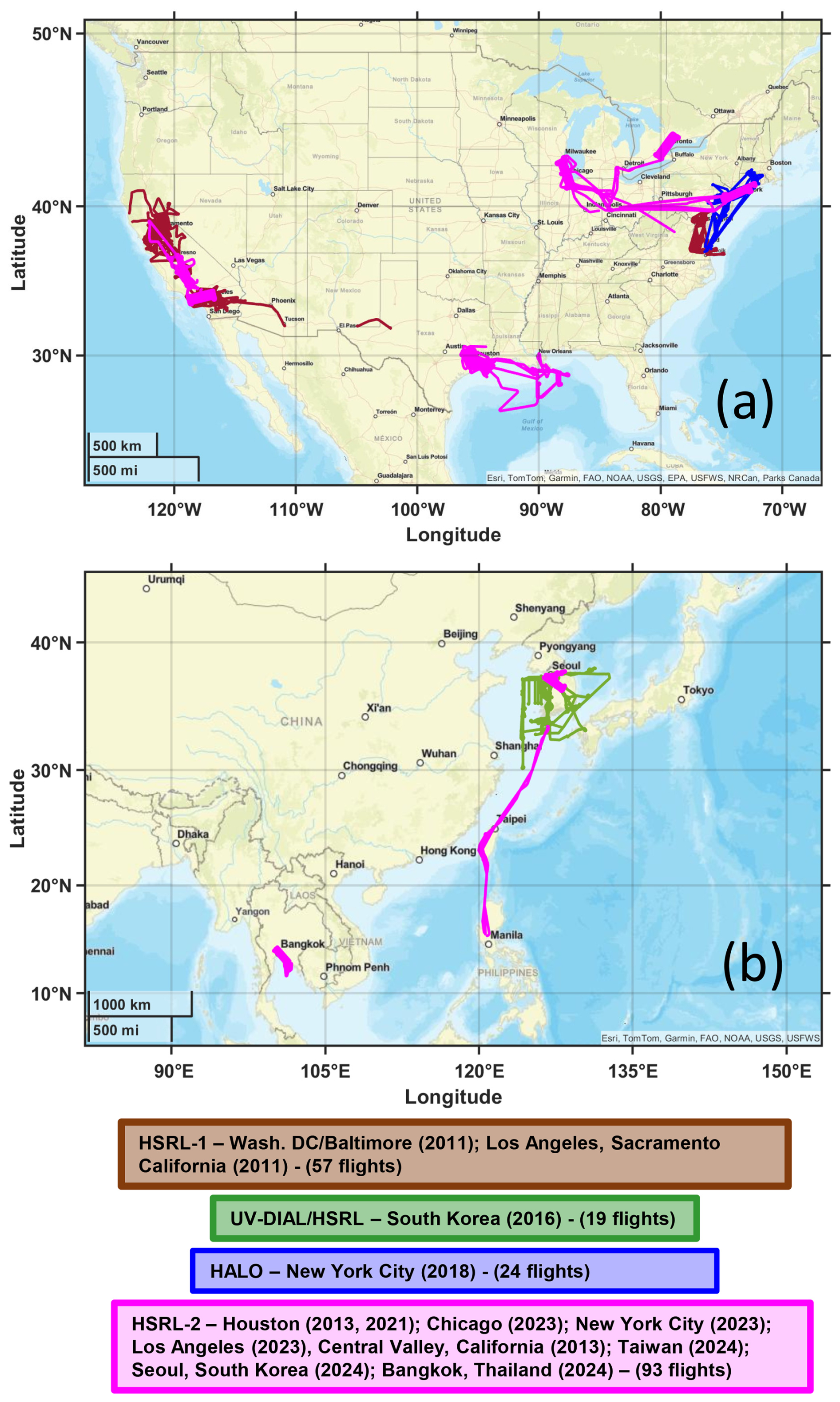
Figure 1 Locations and dates of airborne HSRL measurements over major urban areas in the USA (a) and Asia (b) used in this study. The different colors represent the four different airborne HSRL systems that provided the data used here. Data from 193 flights that occurred between 2010–2024 are used to develop ML algorithms for retrieving PM concentrations. The number of flights conducted by each lidar system is shown at the bottom of the figure.

The raster patterns flown over urban areas in many of these field missions have enabled these systems to acquire data coincident and collocated with surface PM_2.5 and PM₁₀ sensors thereby providing the opportunity to assess how well these surface concentrations can be inferred from airborne remote sensing measurements. Hourly surface PM_2.5 and PM₁₀ data from the US EPA AirNow network (U.S. Environmental Protection Agency, 2017; Toth et al., 2022) as well as similar networks in South Korea, Taiwan, and Thailand were used to examine the relationships among surface PM_2.5 concentrations, AOT, and near-surface aerosol extinction. The PM measurements are acquired via several instruments that follow the Federal Reference Method (FRM; gravimetric analysis) and Federal Equivalent Method (FEM; taper element oscillating microbalance [TEOM] and beta gauge analyses, high volume sampler) regulations (U.S. Environmental Protection Agency, 1997; Noble et al., 2001). Uncertainties in EPA PM_2.5 are summarized in Toth et al. (2019); uncertainties in PM₁₀ are described in Pokhariyal et al. (2019).

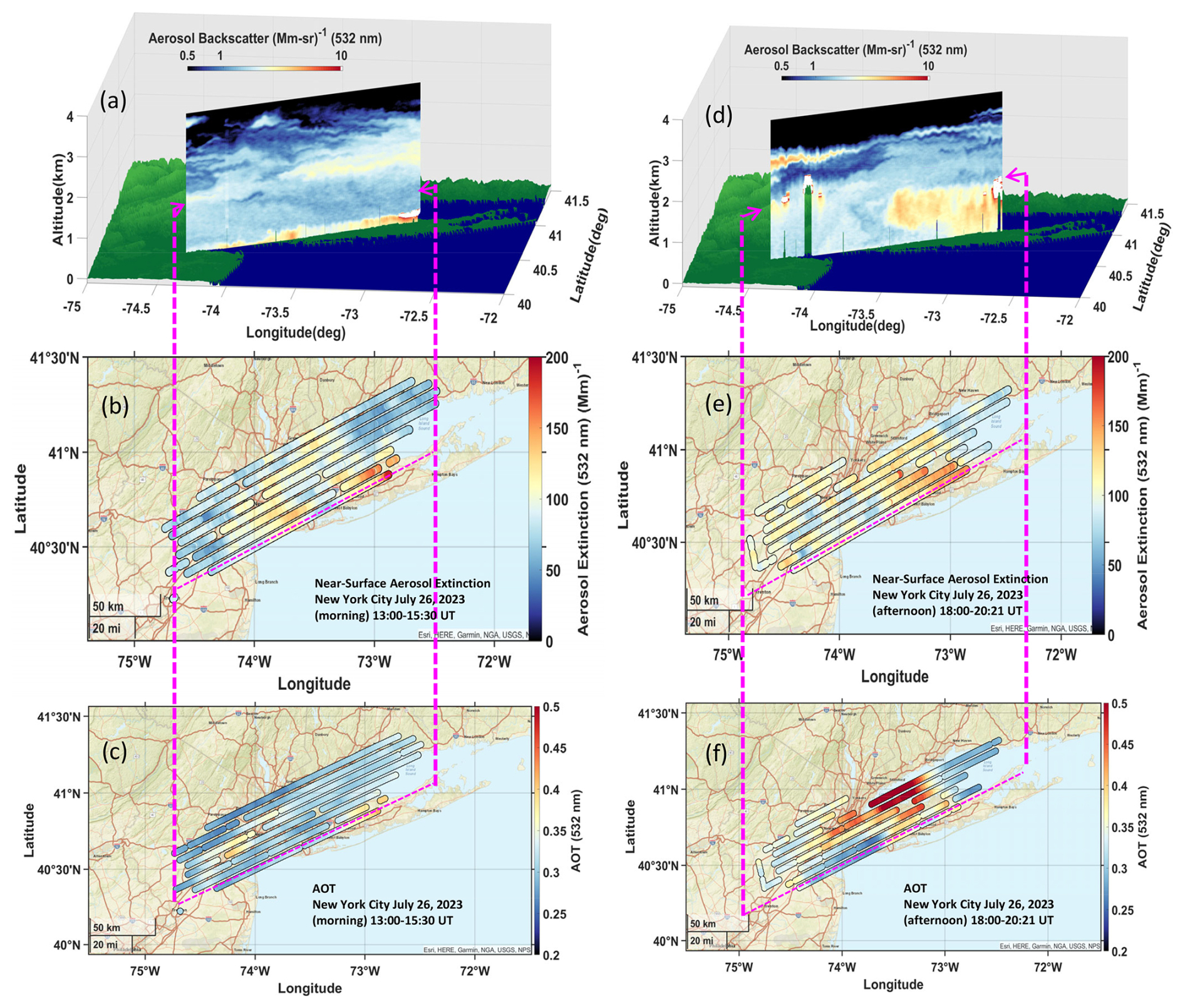
Figure 2 (a) Aerosol backscatter profiles, (b) near-surface aerosol extinction, and (c) AOT measured by airborne HSRL-2 over New York City during the morning of 26 July 2023. Panels (d)–(f) show the same during the afternoon. The dotted lines in panels (b), (c), (e), (f) show the location of the flight legs for the aerosol backscatter profiles shown in panels (a) and (d).

Figure 2 shows examples of HSRL-2 measurements over the New York City metropolitan region on 26 July 2023, when HSRL-2 was deployed on the NASA G-V aircraft. Figure 2a and d show that the vertical distribution of aerosol backscatter (532 nm) varied considerably between the morning and afternoon legs in this pattern. Figure 2a shows the highest aerosol backscatter was located within 100–200 m above the surface. In contrast, Fig. 2d shows a large increase in aerosol backscattering between 1–1.5 km above the surface during the afternoon and the presence of small cumulus clouds at the top of the mixed layer. Figure 2b and e show near-surface aerosol extinction (∼ 300 m thick layer) along this same flight leg for the morning and afternoon flight legs, respectively. Similarly, Fig. 2c and f show AOT for the morning and afternoon legs. These figures illustrate that the spatial and temporal variations in AOT and near-surface aerosol extinction were different on this day.

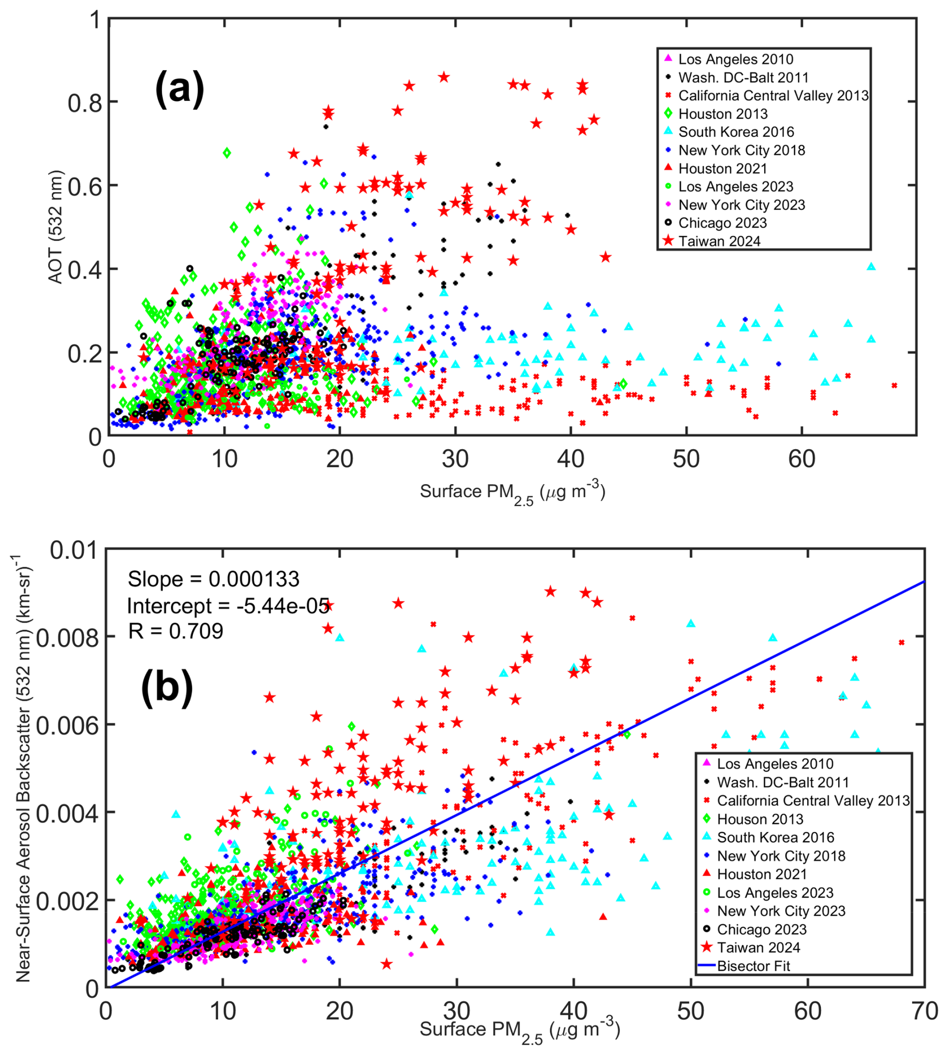
Figure 3 Surface network measurements of PM_2.5 over major metropolitan regions versus airborne HSRL measurements of (a) AOT and (b) near-surface aerosol backscatter. A linear bisector best fit line is shown in panel (b).

Figure 3a shows airborne HSRL measurements of AOT (532 nm) acquired within 10 km and 15 min of the surface PM_2.5 measurements in the urban regions shown in Fig. 1. The overall lack of correlation between AOT and surface PM_2.5 concentrations (correlation coefficient R ∼ 0) is most likely due to differences in the vertical distribution of aerosols among these locations. Elevated aerosol layers were present in all locations except the California Central Valley, where the AOT typically was concentrated in shallow layers near the surface. These elevated aerosol layers impact AOT but not surface aerosol concentrations. This result highlights the difficulty in using column AOT from passive sensors to derive PM_2.5 without accurate knowledge of the vertical distribution of aerosols (Toth et al., 2014, 2019).

Various attempts have been made using boundary layer heights (Liu et al., 2005; Al-Saadi et al., 2008; Chen et al., 2017; Wang et al., 2019; Handschuh et al., 2022) or aerosol layer heights (Chu et al., 2013, 2015) in conjunction with AOT to improve estimates of surface PM_2.5 Scaling the AOT by the MLH that was derived from the HSRL measurements (Scarino et al., 2014) did not significantly improve the overall correlation because in those locations with elevated aerosol layers much of the AOT was located above the MLH. In contrast to Fig. 3a, Fig. 3b shows a much better correlation between HSRL measurements of near-surface aerosol backscatter and surface PM_2.5 concentrations for these same datasets. Near-surface aerosol backscatter represents aerosol backscatter between approximately 60 to 100 m above the surface. For these airborne HSRL datasets, Fig. 3b indicates that the measurements of near-surface aerosol backscatter are more directly related to surface PM_2.5 concentrations than column AOT.

2.3 Machine Learning Regression Algorithms

Based on the results shown in Fig. 3b, we use airborne HSRL measurements of near-surface aerosol properties to retrieve surface PM_2.5 and PM₁₀. For this study, we use ML regression algorithms to estimate PM_2.5 and PM₁₀ concentrations and PM_2.5 $/$ PM₁₀ ratios using these airborne HSRL measurements. Unlike previous methods that have used airborne HSRL data to derive surface PM_2.5 concentrations (Meskhidze et al., 2021; Sutherland et al., 2023; Sutherland and Meskhidze, 2025), this method does not require the HSRL qualitative inferences of aerosol type or aerosol chemical composition information provided by models. We instead take advantage of the large database of coincident HSRL and surface PM_2.5 measurements and machine learning methodology that has used statistical methods to infer surface PM_2.5 from lidar (e.g. Ma et al., 2021; Fang et al., 2021; Chen et al., 2022) and passive sensors (e.g. Lary et al., 2015; Lee et al., 2021; Wang et al., 2023). We use coincident airborne HSRL and surface hourly PM data collected during 193 flights conducted between 2010 and 2024 over major metropolitan regions in the United States (New York City, Houston, Chicago, Los Angeles, Washington D.C., Baltimore) and Asia (Taiwan, South Korea, Thailand) (recall Fig. 1) to explore various machine learning regression models for deriving surface PM concentrations.

We use hourly surface PM measurements from the surface networks described earlier to train machine learning algorithms to retrieve surface PM concentrations from the HSRL measurements. We compute the average of HSRL measurements within 10 km and 15 min of each surface network measurement. The average aerosol backscatter and depolarization values are computed using data within 200 m of the surface and average aerosol extinction values are computed using data within 400 m of the surface. The larger vertical distance is used for aerosol extinction because it has coarser vertical resolution and does not extend as close to the surface as aerosol backscatter and depolarization (recall Table 1). Using the average of the near-surface HSRL measurements within these distance and time constraints rather than each individual HSRL measurement reduces the uncertainties in the HSRL data at each point and reduces number of points used in the training set. This reduction in the number of points consequently reduces the computer time required for subsequent ML regression computations. There are 2382 of these coincident HSRL-surface PM network sets of measurements; approximately 1900 (∼ 80 %) of these sets were randomly chosen to train the regression algorithms. The remaining sets are used to test these algorithms.

We use Matlab regression learner software to explore a variety of various regression methods including linear, random forest, ensemble, neural network, Gaussian process, kernel, and support vector machine. This software enables the user to explore various optimization techniques for these various methods. A five-fold cross-validation method was used to protect against overfitting. For each fold a model is trained using the out-of-fold observations, model performance is assessed using the in-fold data, and the average validation error is computed over all folds. This provides a good estimate of the predictive accuracy of the full data set, which is used to train the final model. The remaining coincident measurements (∼ 500 or 20 %) that were withheld from the training and cross-validation were then used to test these algorithms.

Exponential Gaussian Process Algorithms consistently give the best performance in terms of lowest root-mean-square errors and highest correlations than the other methods. Gaussian process regression (GPR) models are nonparametric, kernel-based probabilistic models based on the assumption that the function to be learned is drawn from a Gaussian process. The GPR model uses Bayesian inference to learn the distribution that is most likely to have generated the data (Williams and Rasmussen, 2006; see also https://apmonitor.com/pds/index.php/Main/GaussianProcessRegression#:~:text=Gaussian%20process%20regression%20(GPR)%20uses,specified%20as%20a%20kernel%20object, last access 19 September 2025). Gaussian process regression has the advantage of providing uncertainty estimates along with point predictions thereby providing a means to quantify the confidence in the predictions. A limitation is that Gaussian process regression can be computationally expensive, especially for large datasets (https://medium.com/@pinakdatta/unlocking-the-power-of-gaussian-processes-theory-applications-and-insights-081d0b6a0abc, last access 19 September 2025).

Table 2 Parameters used in the various exponential GPR ML models.

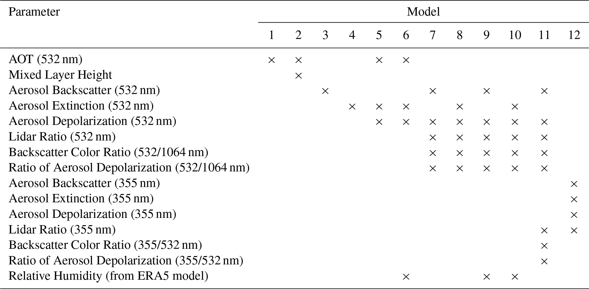
We examined the performance of the exponential GPR models using various combinations of airborne HSRL measurements. Table 2 lists the variables used for each of these different regression models. For example, Model 1 uses only HSRL measurements of AOT (532 nm) whereas Model 11 used a combination of measured near-surface aerosol properties (backscatter, depolarization, lidar ratio) at three wavelengths. As shown in Table 2, most of the model regressions use only these airborne HSRL measurements, although a few of the models also included surface relative humidity provided by ERA5 hourly reanalyses (Copernicus Climate Change Service, 2023; Hersbach et al., 2020); these reanalysis data are gridded to a regular latitude-longitude grid of 0.25°. Since surface PM measurements refer to dry aerosol mass and HSRL aerosol measurements are made at ambient RH, relative humidity is added to these models to assess the impact of including surface relative humidity. Models 7–11 include the lidar ratio and either aerosol backscatter or aerosol extinction since the lidar ratio is the ratio of aerosol extinction to aerosol backscatter.

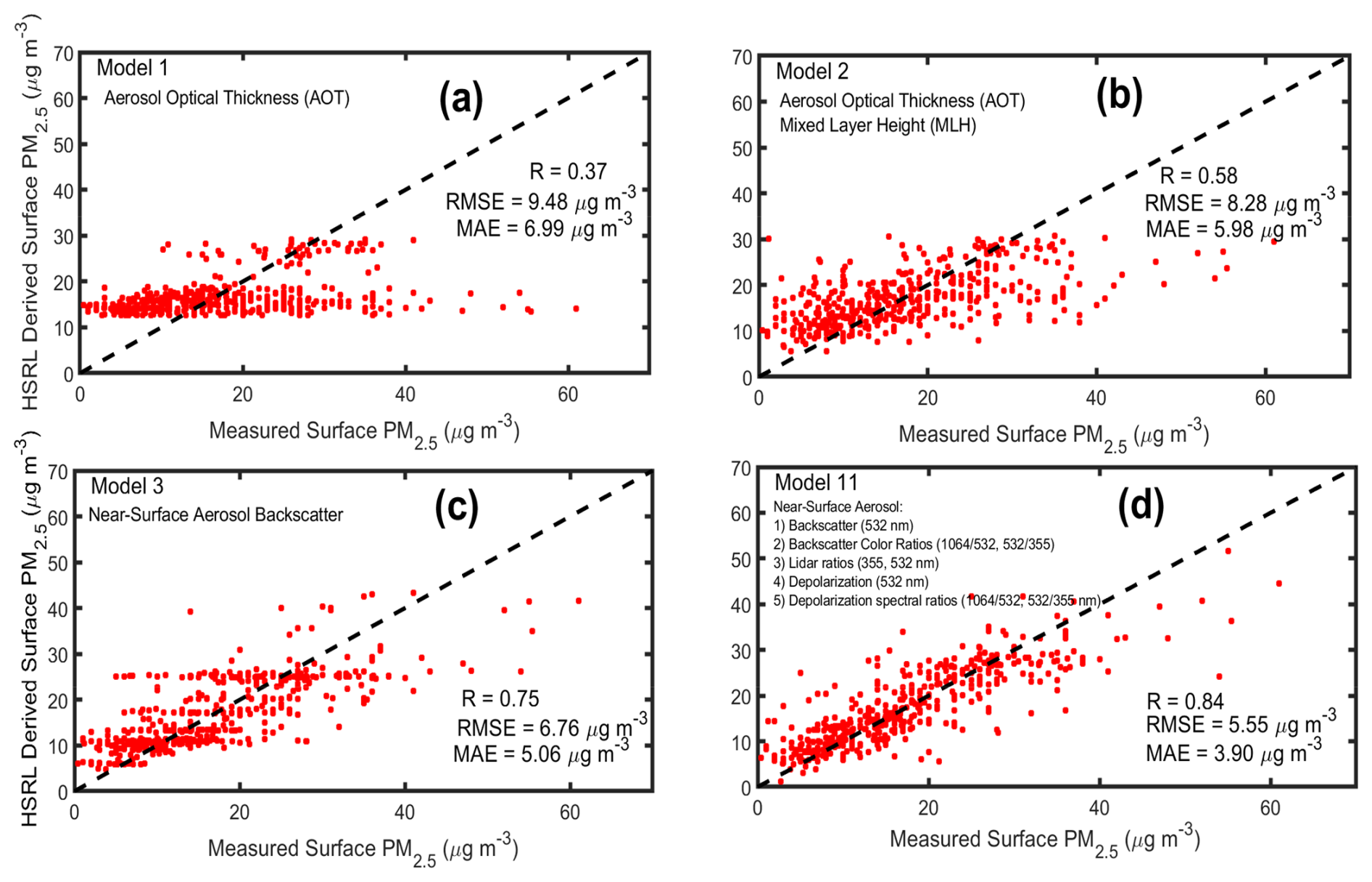
Figure 4 Machine learning exponential Gaussian regression model predictions of surface PM_2.5 using airborne HSRL data versus surface network measurements of PM_2.5 over the major metropolitan regions shown in the legends in Fig. 3. The regression models use various airborne HSRL measurements including (a) AOT (532 nm), (b) AOT (532 nm) and MLH, (c) AOT (532 nm), MLH, and near-surface aerosol backscatter (532 nm), and (d) near-surface aerosol backscatter (532 nm), backscatter color ratio (532/1064 nm), lidar ratio (532 nm), aerosol depolarization (532 nm), and ratio of aerosol depolarizations (532/1064 nm). These results were derived using test data excluded from the training sets.

Figure 4 shows examples of the performance for deriving surface PM_2.5 from various exponential GPR regression models that used airborne HSRL measurements when compared to surface network measurements of PM_2.5. The plots in Fig. 4 also show correlation coefficient, root-mean-square-error (RMSE) and mean absolute error (MAE). Recall that these results were derived using test data withheld from the training and cross-validation sets. As expected from the results shown in Fig. 4, Model 1, which uses only AOT in the GPR ML regression model, performs poorly with a large RMSE error and a low correlation coefficient (Fig. 4a). The poor correlation between AOT and surface PM_2.5 concentrations (correlation coefficient R = 0.37) is most likely due to differences in the vertical distribution of aerosols among these locations. Elevated aerosol layers, which were present in nearly all locations, impact AOT but not surface aerosol concentrations. This result again shows the difficulty in using column AOT from passive sensors to derive PM_2.5 without accurate knowledge of the vertical distribution of aerosols. Scaling the AOT by the MLH provides some improvement to the overall correlation as shown by Model 2 in Fig. 4b; however, the performance is not optimal because in those locations with elevated aerosol layers much of the AOT was located above the MLH. In contrast, model 3 (Fig. 4c) performs significantly better highlighting the benefit of using near-surface aerosol backscatter to infer surface PM_2.5. These near surface lidar measurements of aerosol backscatter were acquired within about 200 m of the surface. The best retrieval performance (i.e., small RMSE and high R) is provided by Model 11 (Fig. 4d), which uses near-surface measurements of aerosol backscatter, aerosol backscatter color ratios (i.e., ratio of aerosol backscatter at 532 nm to that at 1064 nm and the ratio of aerosol backscatter between 355 and 532 nm), aerosol lidar ratios (355, 532 nm), aerosol depolarization (532 nm), and spectral ratios of aerosol depolarization at 532 nm to that at 1064 nm and at 355 to 532 nm. The RMSE (3.79 µg m⁻³) and correlation coefficient (0.84) are considerably better than those from previous studies that used airborne HSRL data in conjunction with models (Meskhidze et al., 2021; Sutherland et al., 2023; Sutherland and Meskhidze, 2025).

The performance of the several exponential GPR models listed in Table 2 that use various combinations of HSRL measurements for retrieving surface PM_2.5 is shown in Fig. 5. These results are derived using test data excluded from the training and cross-validation sets. Although these flights occurred predominantly over urban areas, the aerosols encountered over these areas correspond to several different aerosol types (e.g., urban, smoke, maritime, dust, etc.) as derived from the HSRL aerosol typing algorithm. There were no restrictions on aerosol type nor the PM_2.5 $/$ PM₁₀ ratio when assessing PM concentrations retrieved from the airborne HSRL measurements. Retrieval performance is shown as a function of RMSE and MSE (left axis) and correlation coefficient (right axis). Models 7, 9, 11, and 12, which use some combination of near-surface aerosol backscatter and the aerosol intensive parameters, have the best performance with RMSE generally around 5.4 µg m⁻³ or less and correlation coefficients above 0.8. Performance using only near-surface aerosol backscatter (532 nm) (Model 3) or only near-surface aerosol extinction (Model 4) is generally better than using AOT and MLH (Models 1 and 2). Note also that performance is generally better when using near-surface aerosol backscatter alone (e.g., Model 3) than using near-surface aerosol extinction alone (Model 4). There are (at least) two possible reasons for this. First, aerosol extinction profiles generally have vertical resolutions of between 150–300 m. To avoid contamination from the surface return, the lowest aerosol extinction value is restricted to be generally 200–350 m above the surface. In contrast, the near-surface aerosol backscatter can be derived considerably lower, generally around 60–100 m above the surface, and so will likely be better correlated to surface measurements. Second, HSRL measurements of aerosol backscatter are computed from the ratio of the total (aerosol + molecular) signal to the molecular signal, in contrast to the measurements of aerosol extinction, which are computed from the derivative of the molecular signal (Hair et al., 2008). Computing this derivative leads to more uncertainty than computing the ratio; hence the near-surface aerosol backscatter is less noisy and has generally smaller uncertainties than near-surface aerosol extinction.

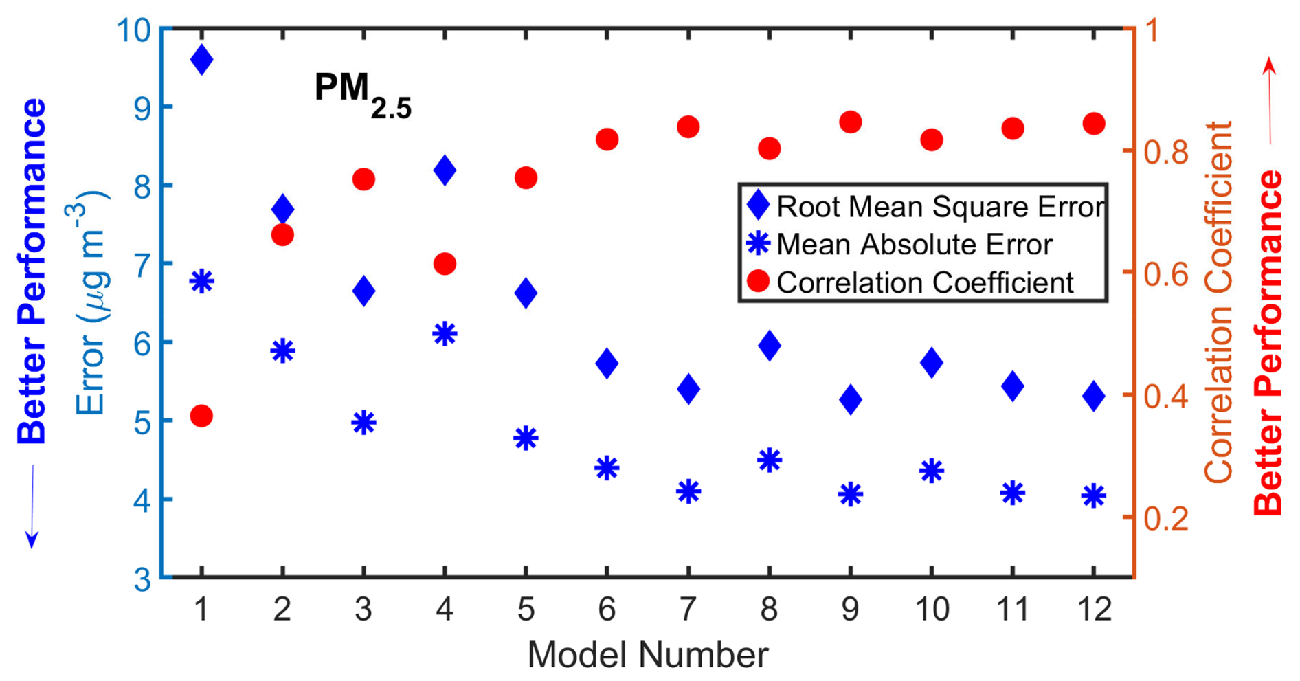
Figure 5 Performance of exponential Gaussian machine learning regression models listed in Table 2 in deriving surface PM_2.5 as measured by RMS and MAE (left axis) and correlation coefficient right axis (right axis) relative to surface PM_2.5 measurements. Performance metrics were derived using data withheld from the training and validation datasets.

Figure 5 shows that performance improves with Models 5 and higher that include aerosol intensive parameters such as aerosol depolarization, lidar ratio, backscatter color ratio, and spectral depolarization ratio. These intensive parameters provide information regarding aerosol composition, shape, and size that improves retrievals of surface PM_2.5. With the addition of these variables, the differences between models using near-surface aerosol backscatter and near-surface aerosol extinction are smaller, i.e., Models 7 vs. 8 and Models 9 vs. 10 have somewhat similar performance. Note that the retrieval performance of Model 11 is about the same as Models 7–10 which indicates that the addition of airborne HSRL aerosol measurements at 355 nm did not significantly improve the PM_2.5 predictive performance. This important result indicates that aerosol measurements at 532 and 1064 nm provided by the airborne HSRL systems that do not include HSRL measurements at 355 nm (i.e., HSRL-1, DIAL/HSRL, and HALO) can be still used to retrieve surface PM_2.5 with the essentially the same retrieval performance as the measurements made by the airborne HSRL-2 system, which includes measurements at 355 nm as well as 532 and 1064 nm. Conversely, note also that the performance of Model 12 is also very similar to that of Models 7–11, which indicates that HSRL measurements of aerosol backscatter, extinction, and depolarization at a single UV wavelength (355 nm) can also be used to retrieve surface PM_2.5. This suggests that lidar systems such as the Atmospheric Lidar (ATLID) on the EarthCARE satellite that operate exclusively at 355 nm can use this methodology to retrieve surface PM_2.5.

It is also interesting to note the performance of Model 5. Of all the models discussed and shown in Table 2, Model 5, which includes measurements of near-surface aerosol extinction, near-surface aerosol depolarization, and AOT and excludes measurements of the lidar ratio and the ratio of aerosol depolarization (532/1064 nm), probably provides the most appropriate configuration to estimate the performance associated with CALIOP. Figures 5 and 6 show that the retrieval performance of Model 5 is not that much worse relative to other models (e.g. 7–11) that included additional parameters as well as Model 12, which corresponds to the ATLID lidar configuration. However, it is important to note that these airborne HSRL systems measure both total attenuated backscatter and total attenuated molecular backscatter to enable direct retrievals of unattenuated aerosol backscatter and aerosol extinction. Since CALIOP did not measure total attenuated molecular backscatter, CALIOP retrievals of aerosol extinction and unattenuated aerosol backscatter typically rely on estimates of the lidar ratio based on inferences of aerosol type. As a result, the CALIOP measurements of near-surface aerosol extinction and, to a lesser extent, near-surface aerosol depolarization can have significant systematic uncertainties due to the uncertainties in the assumed lidar ratios. Consequently, we expect the actual performance of Model 5 as applied to CALIOP retrievals would be worse than the performance as applied to the airborne HSRL systems shown in Figs. 5 and 6.

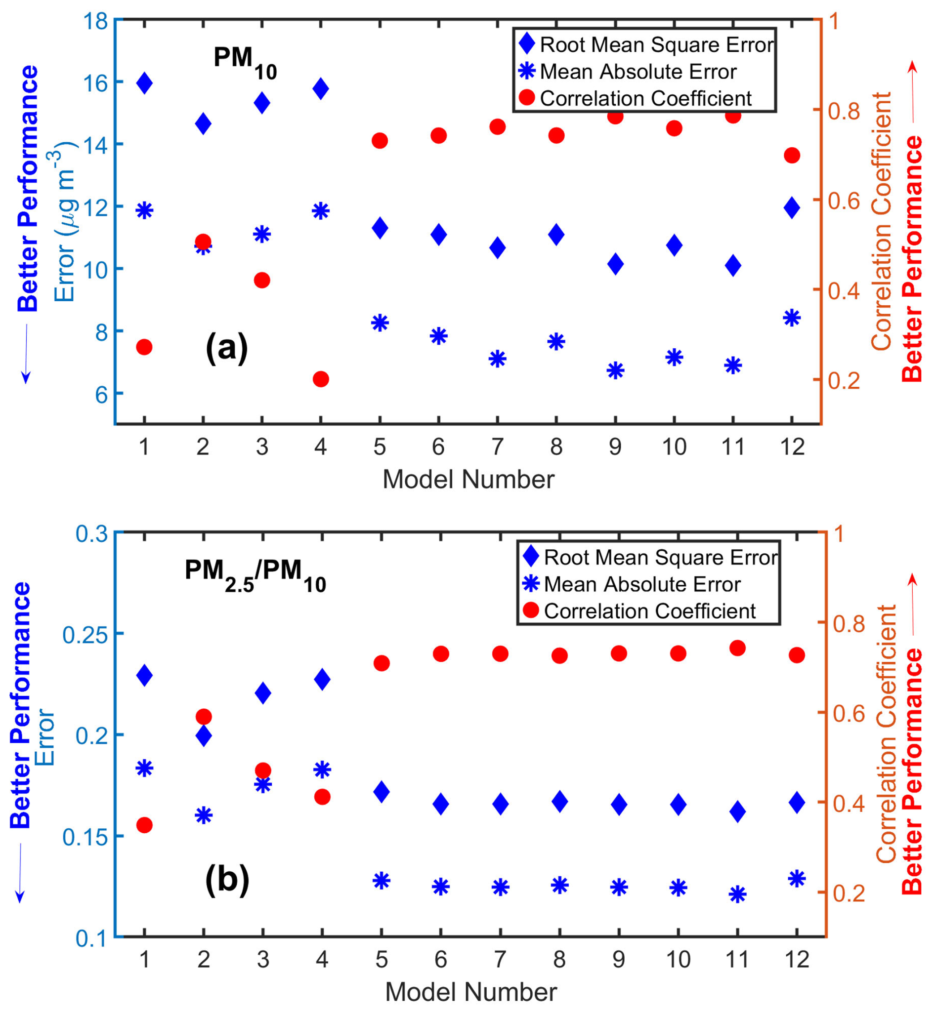
Figure 6 Same as Fig. 5 except showing performance for deriving (a) PM₁₀ and (b) PM_2.5 $/$ PM₁₀. Performance metrics were derived using data withheld from the training and validation datasets.

Except for relative humidity (RH), the model input parameters shown in Table 2 use only airborne HSRL aerosol measurements. Variability in airborne HSRL measurements of near-surface aerosol backscatter and extinction may be due to changes in RH in addition to or instead of changes in dry aerosol mass thereby complicating efforts to use these lidar measurements to retrieve PM_2.5. Therefore, surface RH at the PM_2.5 stations as represented by the ERA5 model is included in Models 6, 9, and 10. Comparing the performance of Models 5 vs. 6, 7 vs. 9, and 8 vs. 10 as shown in Fig. 5 indicates that surface RH provides very little improvement to retrievals of surface PM_2.5 values. One possible reason for this lack of sensitivity is that few (< 10 %) of the surface RH values for these data were above 70 % where increases in aerosol scattering due to hygroscopic growth of the particles are more pronounced. Another reason is that the impact of higher RH is already captured by the behavior of the intensive aerosol parameters measured the airborne HSRL systems. Airborne HSRL measurements of aerosol intensive parameters used in these PM_2.5 retrievals have also been used to retrieve fine mode aerosol number, surface, and volume concentrations and effective radius (Müller et al., 2014; Sawamura et al., 2017; Harshvardhan et al., 2022), real and imaginary refractive index (Wang et al., 2022), aerosol absorption (Redemann and Gao, 2024), aerosol single scattering albedo (Wang et al., 2022), and aerosol shape (Burton et al., 2015; Ferrare et al., 2023). Thus, to the extent that aerosol size, shape, and composition are impacted by changes in RH, the HSRL aerosol intensive properties also respond to and can indicate such changes. For example, aerosol depolarization often decreases with increased RH as particles take on water and become more spherical (Ferrare et al., 2021). Also, changes in particle size due to hygroscopic growth are also indicated by changes in the backscatter color ratio (Su et al., 2008; Burton et al., 2015).

The performance of these exponential GPR models for retrieving PM₁₀ and the ratio of PM_2.5 $/$ PM₁₀ for the various combinations of airborne HSRL aerosol measurements is shown in Fig. 6. The overall predictive performance of PM₁₀ and PM_2.5 $/$ PM₁₀ ratio is somewhat smaller than the performance for PM_2.5. This decrease in performance is likely because typically fine mode aerosols constitute a major part of the aerosol volume; in such cases, accumulation mode aerosols (i.e., PM_2.5 size particles) contribute a larger portion to the total backscatter at the HSRL wavelengths than particles in the coarse mode (i.e. PM₁₀ size particles) (e.g. Müller and Quenzel, 1985; Veselovskii et al., 2004). Measurements of near-surface aerosol backscatter and near-surface aerosol extinction alone are not particularly useful for retrieving PM₁₀ (Fig. 6a) and have poor skill in retrieving the PM_2.5 $/$ PM₁₀ ratio (Fig. 6b). In both cases, performance significantly improves with the addition of aerosol depolarization and, to a lesser extent, other aerosol intensive parameters such as backscatter color ratio. High values of aerosol depolarization are associated with nonspherical particles; dust particles in particular have high aerosol depolarization values (Burton et al., 2012). Nonspherical dust is one of the main types of coarse mode particles, so aerosol depolarization is a particularly useful measurement to indicate the presence of coarse mode particles and for retrieving PM₁₀ and the PM_2.5 $/$ PM₁₀ ratio. Figure 6 shows that the addition of other aerosol intensive parameters such as backscatter color ratio and spectral depolarization ratio provided only marginal improvement when retrieving PM₁₀ and the PM_2.5 $/$ PM₁₀ ratio.

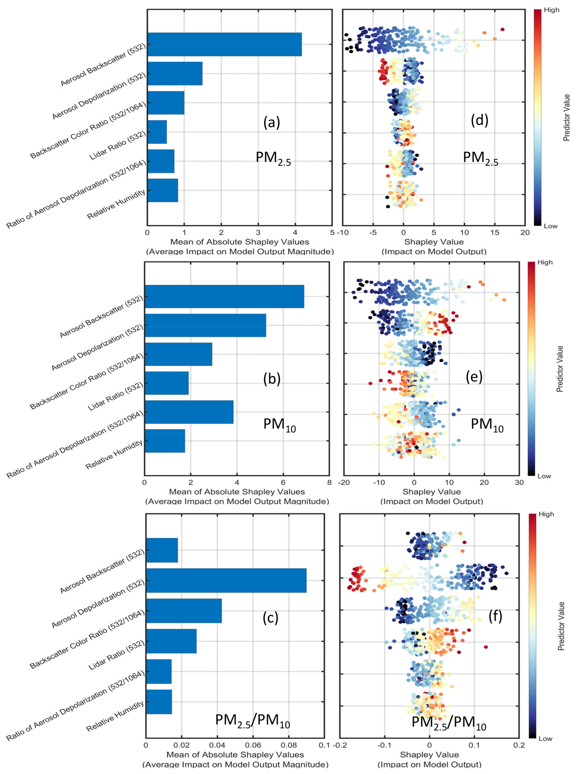
Figure 7 Mean of absolute Shapley values for (a) PM_2.5, (b) PM₁₀, and (c) PM_2.5 $/$ PM₁₀. These values identify which predictors have the largest or smallest average impact on predicted response values. Summaries of the Shapley values according to its predictor value for (d) PM_2.5, (e) PM₁₀, and (f) PM_2.5 $/$ PM₁₀. The Shapley value of a variable for a particular point explains the deviation of the prediction for that point from the average prediction, due to the predictor. The sign of the Shapley value indicates the direction of this deviation, and the absolute value indicates its magnitude.

Figure 7 shows the importance and relationship of the various parameters to retrievals of PM_2.5, PM₁₀, and the PM_2.5 $/$ PM₁₀ ratio as represented by Shapley scores for Model 9. Shapley values show the relative average impact of each variable on the retrieval and so identify which variables have the largest or smallest average impact on retrieved values (https://www.mathworks.com/help/releases/R2025a/stats/ explain-model-predictions-for-regression-models-trained-in-regression-learner-app.html#mw_9aa6a89c-835c-47fc-b1ec-68ce31e14505, last access: 12 September 2025). Figure 7a, b, and c show the mean of the absolute Shapley values for each variable and thus show a measure of each variable's importance for model retrievals. Figure 7d, e, and f show summaries of the Shapley values for each query point according to its retrieval value. The Shapley value of a variable for a particular point explains the deviation of the retrieval for that point from the average retrieval, due to the variable. The sign of the Shapley value indicates the direction of this deviation, and the absolute value indicates its magnitude. Shapley values near zero indicate that the variable has a minimal impact on the model retrievals for that query point. High Shapley values (orange and red) such as for aerosol backscatter (532 nm) in Fig. 7d and e indicate that high aerosol backscatter values correspond to a larger retrieved surface PM_2.5 and PM₁₀ values. Conversely, lower backscatter values (blue) correspond to lower retrieved surface PM_2.5 and PM₁₀ values. Note how the Shapley values for aerosol depolarization (532 nm) differ in behavior for retrievals of PM_2.5 and PM_2.5 $/$ PM₁₀ ratio vs. PM₁₀. High values of aerosol depolarization that are associated with nonspherical coarse mode dust particles correspond to lower retrieved values of PM_2.5 (and lower PM_2.5 $/$ PM₁₀ ratio) but higher retrieved values of PM₁₀. These figures again show how aerosol backscatter (532 nm) dominates the retrievals of PM_2.5 and the increasing contribution of aerosol depolarization and other intensive parameters for retrievals of PM₁₀. Since the PM_2.5 $/$ PM₁₀ ratio is an aerosol intensive parameter providing a measure of aerosol size, aerosol intensive parameters such as aerosol depolarization and backscatter color ratio have a greater impact on this ratio than an extensive parameter such as aerosol backscatter. This figure also shows the relatively small impact of relative humidity on retrievals of PM_2.5 and the negligible impact on predictions of PM₁₀ and PM_2.5 $/$ PM₁₀.

It is important to note that these GPR model results for PM_2.5, PM₁₀, and PM_2.5 $/$ PM₁₀ apply to the ranges of PM_2.5, PM₁₀, and PM_2.5 $/$ PM₁₀ present in the training set. These ranges were: 2–80 µg m⁻³ for PM_2.5, 5–110 µg m⁻³ for PM₁₀, and 0.01–0.98 for PM_2.5 $/$ PM₁₀. The ranges of HSRL aerosol measurements in these training sets were: 0.1–12 (Mm sr)⁻¹ for aerosol backscatter (532 nm), 5–500 Mm⁻¹ for aerosol extinction (532 nm), 0.01–0.3 (1 %–30 %) for aerosol depolarization (532 nm), 15–80 sr for the lidar ratio (532 nm), and 0.05–4 for the aerosol backscatter color ratio (532 m/1064 nm). The specific training set used here would be suitable for retrieving PM estimates for PM values and HSRL aerosol measurements in these ranges but would not be suitable for retrieving PM significantly higher than the maximum values listed above. Based on additional tests we conducted, in such cases of high PM concentrations the current training set likely would lead to underestimates in the retrieved PM values. However, if additional HSRL aerosol measurements and coincident surface PM measurements associated with higher PM values become available, a revised training set using those measurements could be readily developed for determining revised GPR models that could then be used for such PM retrievals.

3 Results

3.1 STAQS and ASIA-AQ missions

We demonstrate the use of this ML methodology to retrieve surface PM_2.5 values using airborne HSRL-2 data collected during the NASA Synergistic TEMPO Air Quality Science (STAQS, https://www-air.larc.nasa.gov/missions/staqs/, last access: 15 August 2025) and Airborne-Satellite Investigation of Asian Air Quality (ASIA-AQ, https://www-air.larc.nasa.gov/missions/asia-aq/, last access: 10 September 2025) missions. The STAQS mission was conducted to integrate Tropospheric Emissions: Monitoring of Pollution (TEMPO) satellite observations with traditional and enhanced air quality monitoring to improve the understanding of air quality science for increased societal benefit (Judd et al., 2022). STAQS objectives include the evaluation of TEMPO retrievals of trace gases and assessments of benefits of assimilating TEMPO data into chemical transport models. STAQS conducted flights over major metropolitan areas in the United States during July and August 2023 including Los Angeles, Chicago, and New York City. During the STAQS mission HSRL-2 was deployed on the NASA JSC G-V aircraft which flew raster patterns from an altitude of about 9 km over these cities. Each raster pattern had about 10 legs with each leg separated by about 8 km. Each leg was about 140 km long and took about 12 min to complete so the entire raster pattern took around 2 to 2.5 h. During each 8 h flight, the G-V typically flew three raster patterns which allowed HSRL-2 to measure profiles of aerosols and ozone and derive PM concentrations along these raster patterns during the morning, mid-day, and afternoon.

The overarching goals of ASIA-AQ are to improve: (1) the integration of satellite observations with existing air quality ground monitoring and modeling efforts across Asia, (2) the understanding of the factors controlling local air quality across Asia. Specific goals involved measurements relating to: satellite validation and interpretation, emissions quantification and verification, model evaluation, aerosol chemistry, and ozone chemistry (Crawford et al., 2022). ASIA-AQ conducted airborne sampling across multiple locations during February and March 2024 with flights over Manila (Philippines), Taiwan, Seoul (South Korea), and Bangkok (Thailand). NASA deployed two aircraft for ASIA-AQ: (1) the LaRC G-III aircraft with HSRL-2 to measure profiles of aerosols and ozone and the GEO-CAPE Airborne Simulator (GCAS) instrument to measure column densities of nitrogen dioxide and formaldehyde, and (2) the DC-8 aircraft with a suite of in situ instruments to measure trace gas and aerosol composition. During ASIA-AQ the G-III flew at about 9 km in raster patterns over each metropolitan region. These raster patterns were like those flown during STAQS except that the shorter endurance of the G-III required two separate flights to achieve three raster patterns; two raster patterns were completed during the first flight and another raster pattern was completed during the second flight. Because of the longer transit times, only single raster patterns were flown over Taiwan on each of the 4 d.

Measurements of aerosol size, composition, scattering and absorption coefficients were acquired by in situ instruments on the DC-8 during ASIA-AQ. Sub-micrometer non-refractory aerosol chemical composition (sulfate, nitrate, ammonium, organics, and chlorine) was measured by a High-Resolution Time-of-Flight Aerosol Mass Spectrometer (HR-ToF-AMS) manufactured by Aerodyne Research (Guo et al., 2021; Kim et al., 2025). A Single Particle Soot Photometer (SP2) measured sub-micrometer refractory black carbon mass. A TSI nephelometer (Model 3563) measured sub-micrometer aerosol scattering coefficients and a particle soot absorption photometer (PSAP, Radiance Research, Inc.) measured sub-micrometer aerosol absorption coefficients. Aerosol dry size distributions between 3 and 100 nm (diameter) were measured by a TSI, Inc. Scanning Mobility Particle Sizer (SMPS, Differential Mobility Analyzer model 3085) (Moore et al., 2017); a Droplet Measurement Technologies Ultra-High Sensitivity Aerosol Spectrometer (UHSAS) measured dry aerosol size distributions between 100 and 1000 nm (diameter) (Moore et al., 2021) and Aerodynamic Particle Sizer (APS, TSI model 3321) provided measurements between about 1000 and 3000 nm.

Dry PM_2.5 concentrations and fine mode Mass Extinction Efficiency (MEE_f) are derived from these DC-8 measurements in the following manner. Size distributions from the SMPS, UHSAS, and APS are converted to geometric diameter and then stitched together following (Soloff et al., 2024) to derive the volume concentration for particle diameters less than 2.5 µm. Then, bulk fine mode non-refractory aerosol density is estimated from HR-ToF-AMS and SP2 black carbon measurements (Saide et al., 2022) by means of mass weighting and then used to derive dry PM_2.5 mass concentrations. Additional details on the density computations are provided by Salcedo et al. (2006) and Kuwata et al. (2012). These estimates of PM_2.5 concentrations are quality assured by removing them whenever the HR-ToF-AMS+SP2 aerosol mass measurements are not existent (i.e., cloud contaminated) or when these estimates of PM_2.5 concentrations derived from the size distribution are at least three times larger than those derived from the HR-ToF-AMS+SP2 mass. In-situ dry aerosol extinction at 532 nm is derived from the measurements of aerosol scattering and absorption (Ziemba et al., 2013). Finally, dry MEE_f is derived from the ratio of extinction and PM_2.5.

3.2 PM_2.5, PM₁₀, and PM_2.5 $/$ PM₁₀ retrievals

Figure 8 shows examples of retrievals of surface PM_2.5, PM₁₀, and PM_2.5 $/$ PM₁₀ derived over the New York City (NYC) metropolitan region on 26 July 2023, during the STAQS mission. HSRL-2 was deployed from the NASA G-V aircraft which flew this raster pattern three times during an approximate 8 h flight over the NYC region. These values were derived using the Model 11 regression. The HSRL-2 surface PM retrievals show extensive temporal and spatial variability. Note how the location of the highest surface PM_2.5 varies during the day between eastern Long Island and central New York City. Interestingly, high surface PM_2.5 was derived over Long Island Sound during the morning. Corresponding surface values measured by EPA surface stations are also shown; these measurements were acquired using instruments as per the Federal Reference Method (FRM; gravimetric analysis) and Federal Equivalent Method (FEM; taper element oscillating microbalance [TEOM] and beta gauge analyses) regulations (Federal Register, 2009; Greenstone, 2002). This figure shows that the HSRL-2 retrievals provide considerable additional spatial and vertical information unavailable from the surface sensors.

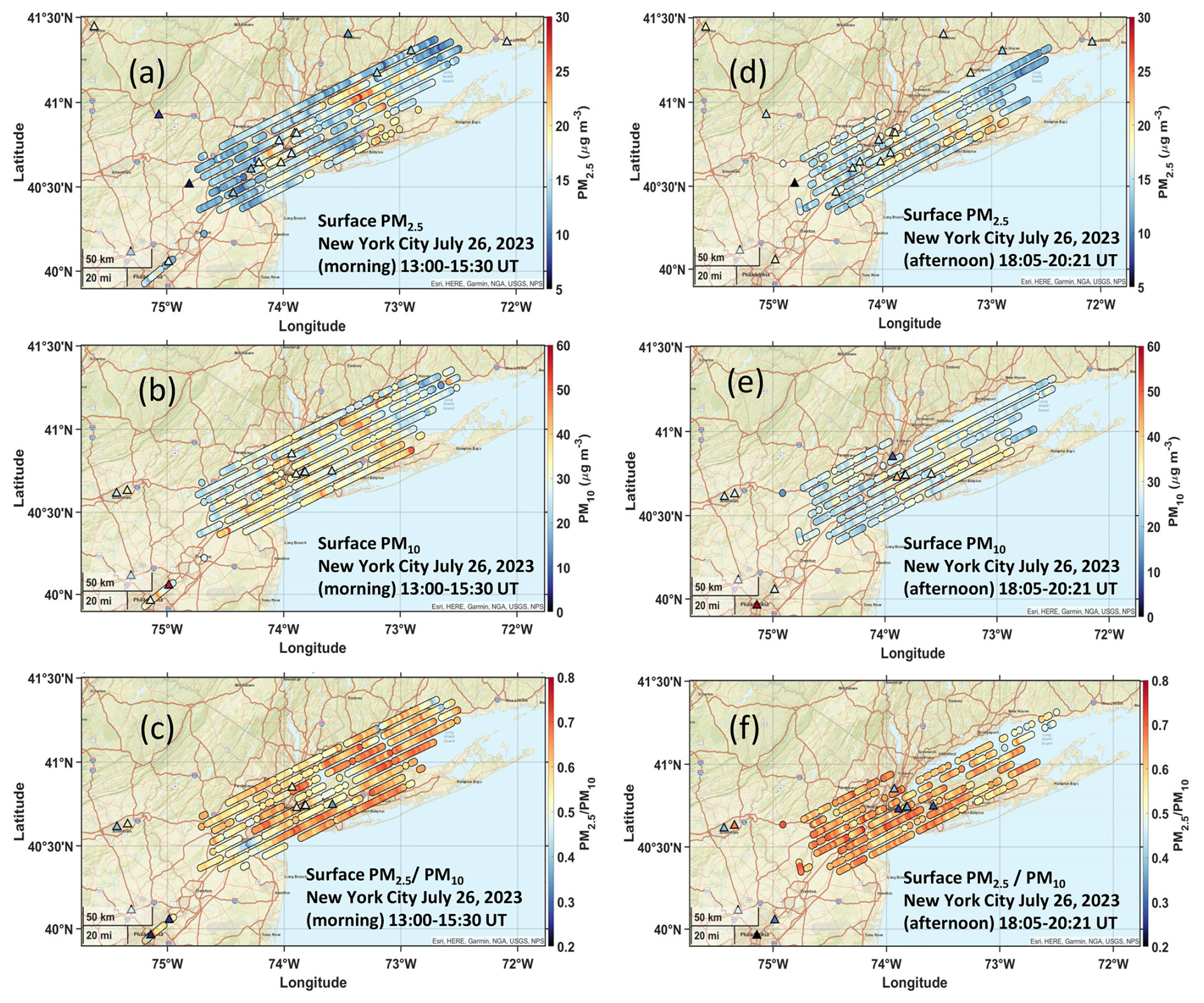
Figure 8 (a) Surface PM_2.5, (b) PM₁₀, and (c) PM_2.5 $/$ PM₁₀ derived from airborne HSRL-2 data acquired over New York City during the morning of 26 July 2023. Panels (d)–(f) show the same during the afternoon. Corresponding surface values measured by EPA surface stations are also shown as triangles.

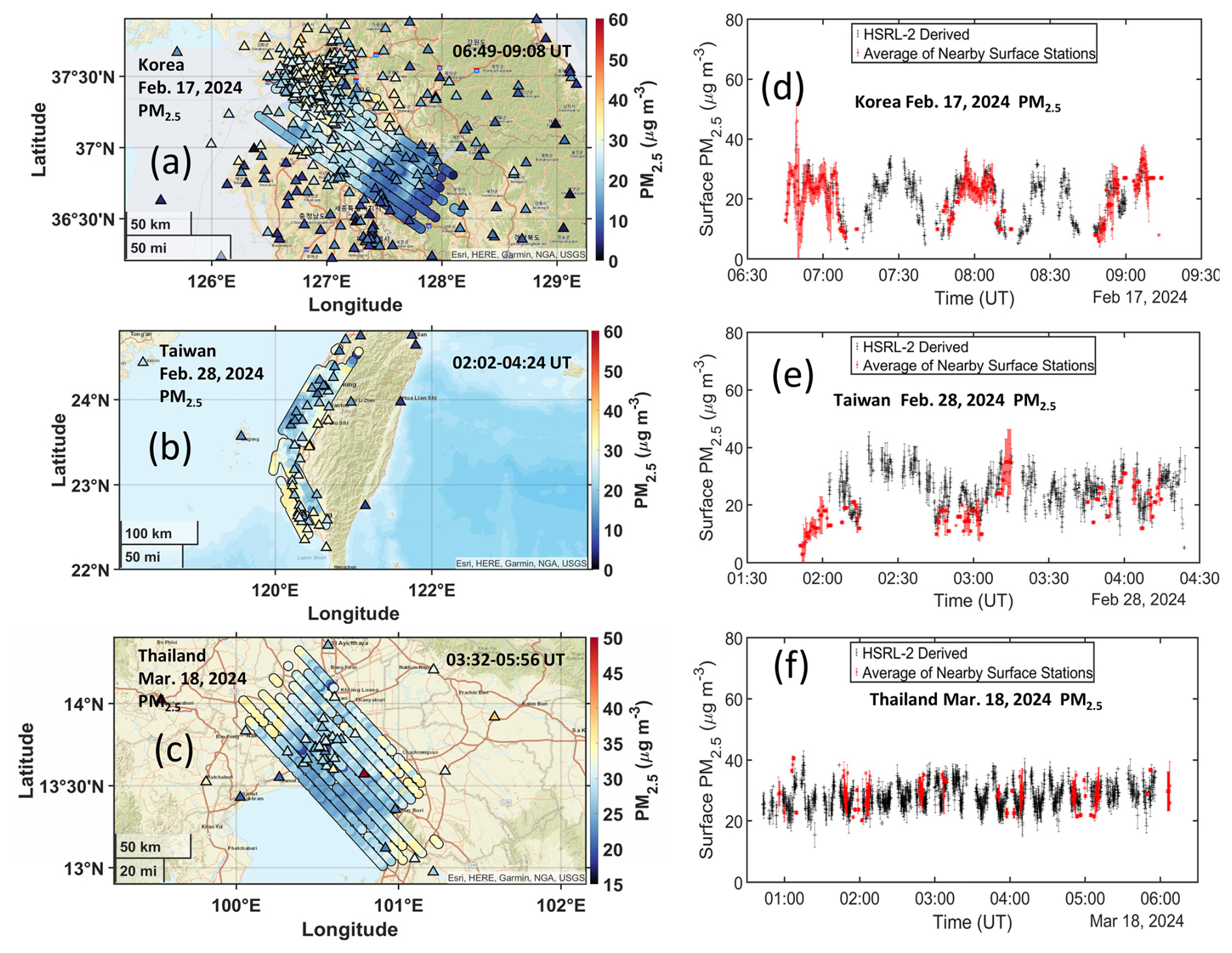
Figure 9 Surface PM_2.5 derived from airborne HSRL-2 measurements acquired during raster patterns over South Korea (a), Taiwan (b), and Thailand (c). The colored triangles also show surface PM_2.5 values measured by surfaced stations during the HSRL-2 measurements. Corresponding plots showing surface PM_2.5 derived from airborne HSRL-2 measurements and measured by surface stations as a function of time (UT) during these flights are also shown in panels (d)–(f).

Figure 9 shows examples of surface PM_2.5 derived from HSRL-2 measurements acquired over South Korea, Taiwan, and Thailand during ASIA-AQ. The left panels (Fig. 9a, b, c) show the spatial distribution of PM_2.5 during each of these flights. Also shown are average surface network PM_2.5 measurements during the raster. Figures 10 and 11 show HSRL-2 retrievals of PM₁₀ and PM_2.5 $/$ PM₁₀ and corresponding surface PM measurements for these regions. The HSRL-2 retrievals of surface PM_2.5 show considerable spatial variability in surface PM_2.5 over these sites. Figures 9a and 10a show highest surface PM_2.5 and PM₁₀ values occurred over Seoul with lower concentrations over rural areas southeast of Seoul. Figure 11a shows that the highest values of PM_2.5 $/$ PM₁₀ ratio corresponding to smaller particles also occurred over this urban region of Seoul. Figures 9b, 10b, 11b show higher PM_2.5 and PM₁₀ concentrations and higher PM_2.5 $/$ PM₁₀ values in the urban areas between Tainan and Kaohsiung on the southwestern coast of Taiwan. Figures 9c, 10c, 11c show highest concentrations of surface PM_2.5 and PM₁₀ occurred slightly to the northwest and southeast of Bangkok with lower concentrations over the Gulf of Thailand south of Bangkok. Figure 9d, e, f show the HSRL-2 retrievals of surface PM_2.5 during these raster patterns along with the averages of surface PM_2.5 measurements within 15 min and 10 km of the HSRL-2 measurements. These also show examples of the variability in surface PM_2.5 over these urban regions. These figures also show that the HSRL-2 surface PM_2.5 retrievals and the surface PM_2.5 measurements acquired over these regions were in good agreement. Figures 10d, e, f and 11d, e, f show corresponding HSRL-2 retrievals of surface PM₁₀ and PM_2.5 $/$ PM₁₀, respectively, during these raster patterns.

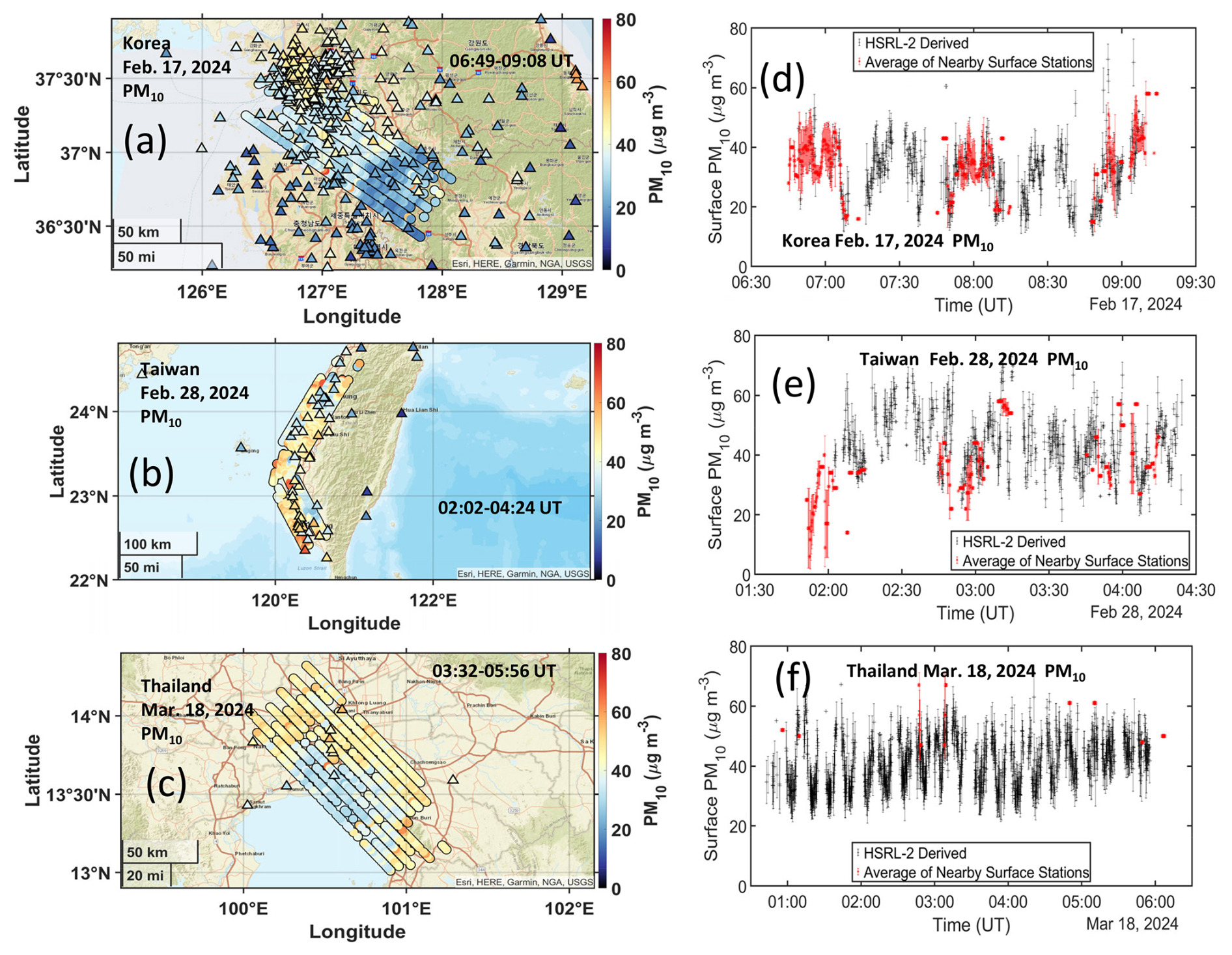
Figure 10 Same as Fig. 9 except for surface PM₁₀.

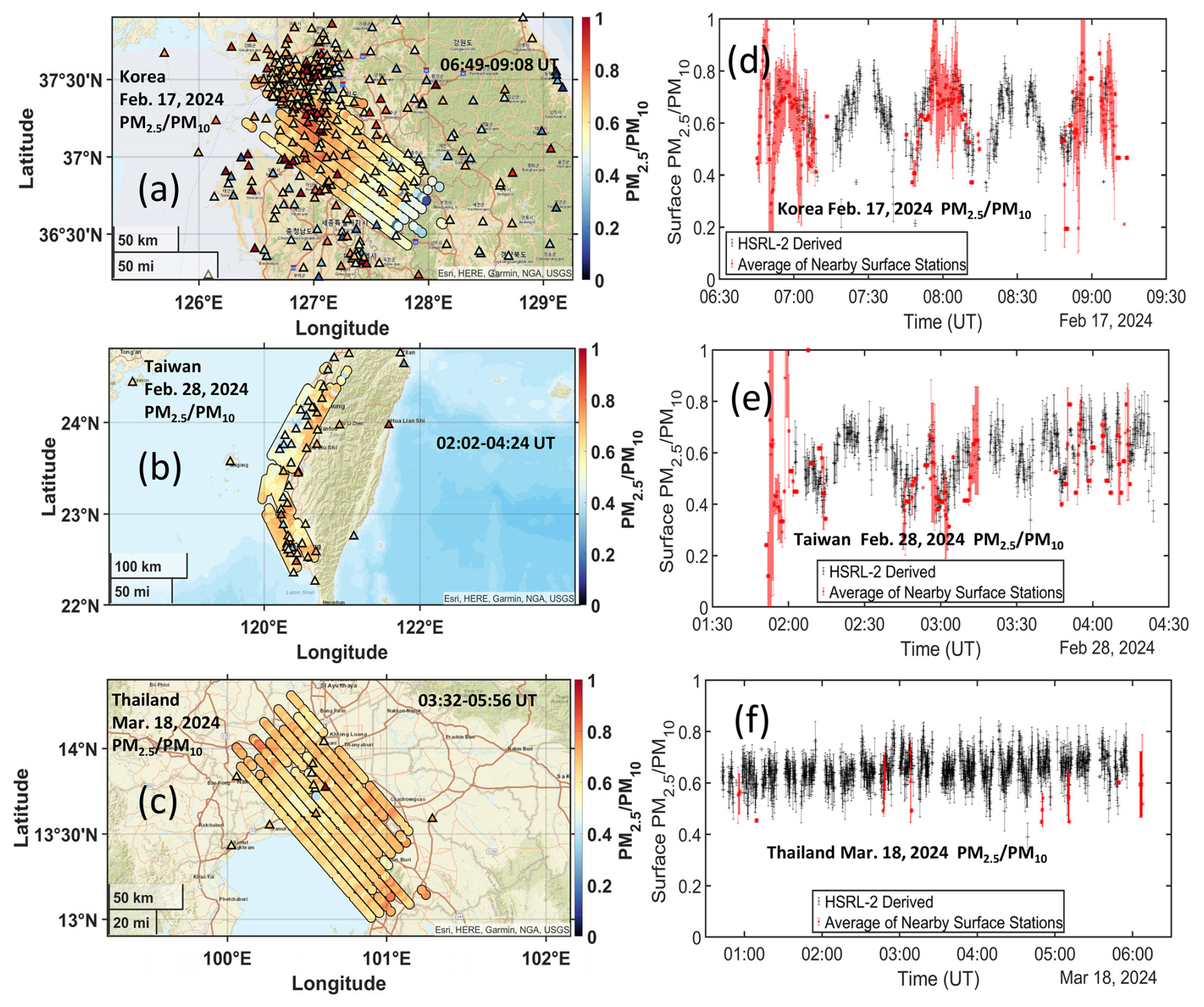
Figure 11 Same as Fig. 9 except for surface PM_2.5 $/$ PM₁₀.

3.3 PM comparisons and sensitivity studies

Overall comparisons of the HSRL-2 surface PM_2.5 retrievals and the surface PM_2.5 measurements for all HSRL-2 surface PM_2.5 retrievals during the STAQS and ASIA-AQ missions are shown in Figs. 12 and 13, respectively. Note that these figures show surface PM_2.5 derived from each HSRL measurement within 10 km and 15 min of a single surface network PM_2.5 measurement rather than PM_2.5 derived from the average of all HSRL measurements within this same distance and time requirement; consequently, there are many more points that are used for these comparisons than were used in the training set (i.e., Fig. 4). Mean absolute error (MAE) and root-mean-square-error (RMSE) differences between the HSRL-2 surface PM_2.5 retrievals and the surface PM_2.5 measurements are shown along with linear bisector slope, intercept, and correlation coefficient in each case.

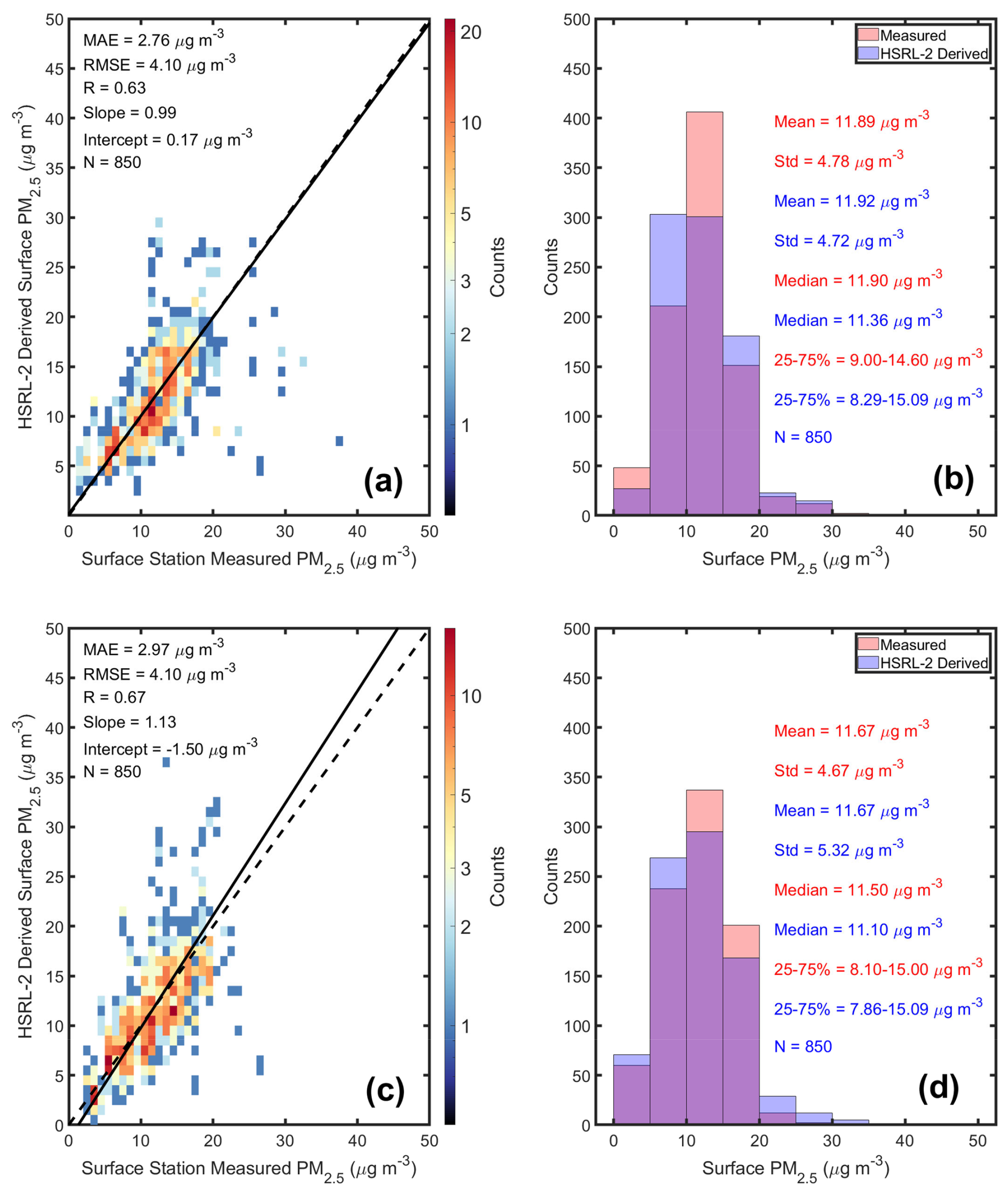
Figure 12 Regression (a) and histogram (b) comparisons of surface PM_2.5 derived from airborne HSRL-2 measurements and measured by surface stations during the NASA STAQS mission (2023). STAQS data were included in the training set. Panels (c) and (d) are the same except using a model that used the same parameters and a training set that excluded data from the STAQS mission.

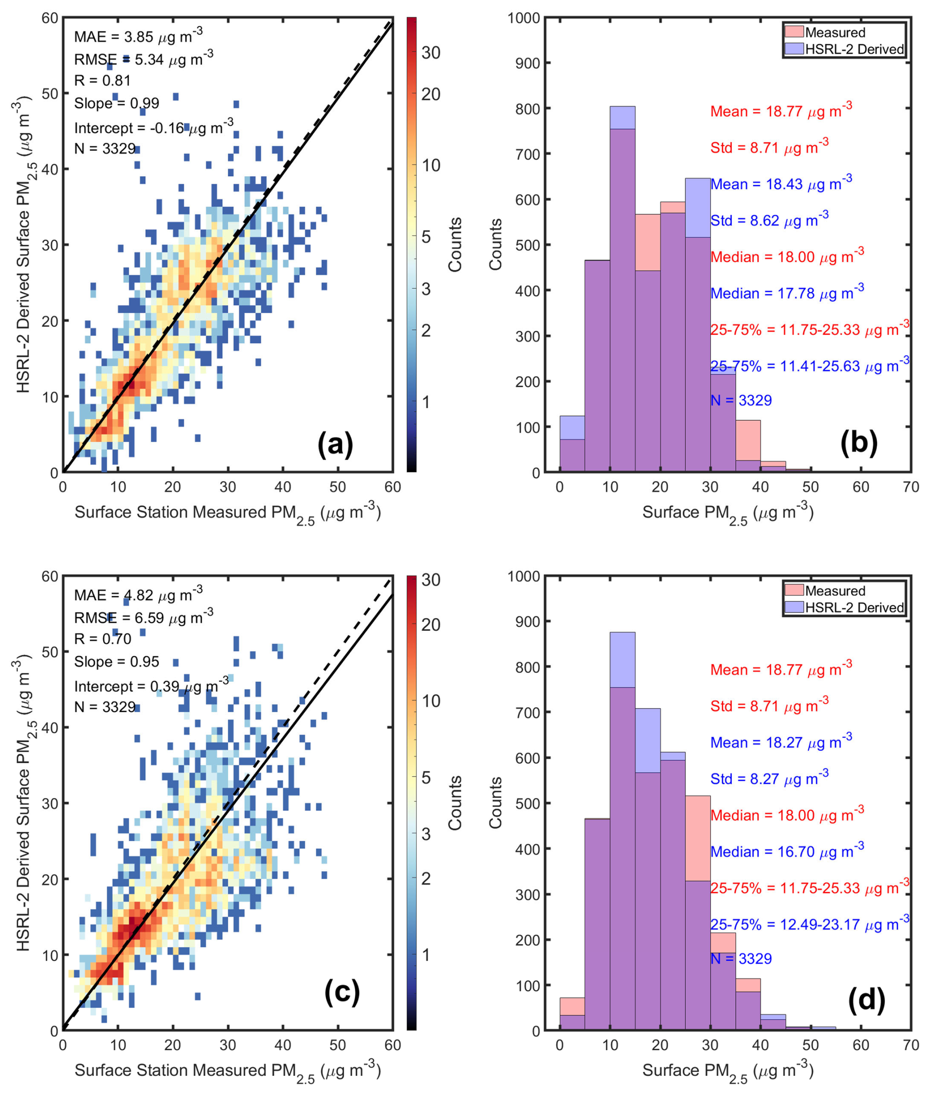
Figure 13 Same as Fig. 12 except for the ASIA-AQ mission; panels (a) and (b) correspond to results where ASIA-AQ data were included in the training set and panels (c) and (d) correspond to results where ASIA-AQ data were not included in the training set.

Figure 12a and b show results from the STAQS mission retrieved from Model 11 that used the training set that included data from the STAQS mission. Approximately 12 % of the data used in the training set were from the STAQS mission; the remaining training set data are from other field missions including ASIA-AQ. Figure 12c and d show results from Model 11 that used a different training set that excluded data from the STAQS mission. Thus, the results shown in Fig. 12c and d provide an example of the use of a training set as applied to a new set of measurements. Comparing the retrieval results between the top and bottom panels in Fig. 12 shows that excluding STAQS data from the training set did not affect the retrieval performance when applied to the STAQS data. This indicates that the relationships among the HSRL aerosol measurements and the surface PM_2.5 concentrations and the range of PM_2.5 concentrations observed during STAQS was not appreciably different from those observed during the other missions.

Figure 13a and b show similar results from the ASIA-AQ mission using Model 11 and the training set that included data from the ASIA-AQ mission; Fig. 13c and d show results from Model 11 that used another training set that excluded data from the ASIA-AQ mission. Since nearly half (48 %) of the data used in the original training set were from the ASIA-AQ mission, this represents a more extreme test than the exclusion of STAQS training set data discussed above. Note that ASIA-AQ contributed this much larger fraction of data to the training set due to the higher density of surface network ground stations in these locations (e.g. Seoul, South Korea; Taiwan in particular) as compared surface station density to the United States. This test may be somewhat unrealistic, but it does provide an interesting and drastic case where the method is applied to large amount of new data that have not been included in the training set. Such a case may arise when there are no coincident surface network PM measurements available to add to the training set. Comparing the results between the top and bottom panels in Fig. 13 shows that excluding ASIA-AQ data from the training set produced only a modest degradation in retrieval performance. Given that ASIA-AQ contributed a large fraction of the data to the training set, this result shows that the methodology is relatively insensitive to changes in the size of the training set assuming that the remaining training data still adequately reflect the relationships among the HSRL aerosol measurements and the surface PM_2.5 concentrations. However, when confronted with a large amount of new data, we recommend, if possible, to include some of these new measurements as additional training data for optimal retrieval performance.

We also compared PM_2.5 derived from the HSRL-2 data acquired during the ASIA-AQ mission with PM_2.5 derived from the DC-8 in situ instruments as described in Sect. 3.1. Recall PM_2.5 was retrieved from the DC-8 measurements using particle size distributions measured by the SMPS, UHSAS, and APS instruments and particle density measured by the AMS and SP2 instruments. In addition to providing another independent comparison of PM_2.5, this exercise provides a way to examine HSRL-2 retrievals of PM_2.5 aloft as well as near the surface. The HSRL-2 retrievals of PM_2.5 aloft used for this comparison are determined in the same manner as the near-surface values such that the profiles of aerosol backscatter, depolarization, lidar ratio, etc. measured by HSRL-2 are used in the same ML regression algorithm that is used to derive near-surface PM_2.5. PM_2.5 retrieved from DC-8 at one-second frequency was matched to HSRL-2 measurements that were within 5 km horizontally and 30 min using software previously developed for this purpose (Schlosser et al., 2024). Since HSRL-2 provides vertically resolved measurements, the closest retrieval to the DC-8 altitude was used for each profile. We then examined results after aggregating to 1 min averages of the matched data. Figure 14 shows that the HSRL and DC-8 in situ PM_2.5 retrievals aloft are in good agreement with correlations and MAE and RMS differences that are comparable to those found when comparing the HSRL retrievals of surface PM_2.5 to PM_2.5 measured by the surface network instruments.

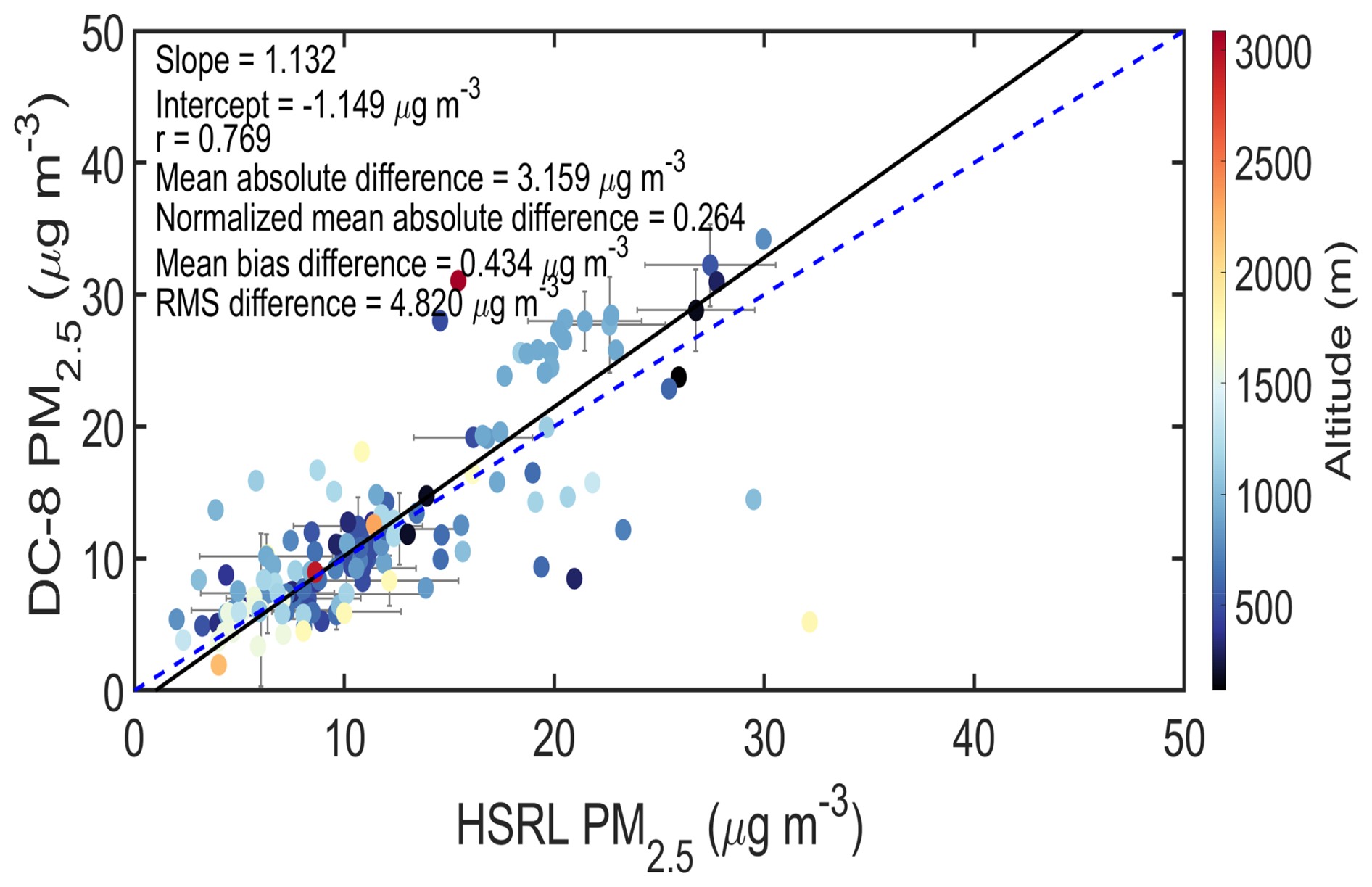
Figure 14 Comparison of PM_2.5 derived from ML regression algorithms using HSRL-2 data (x axis) vs. PM_2.5 derived from DC-8 in situ instruments (y axis) during the ASIA-AQ mission. Results are color-coded by altitude. The solid line represents a least-squares bisector fit and the dashed line represents the 1 : 1 line. Error bars represent the two standard deviations derived from the 1 min averages.

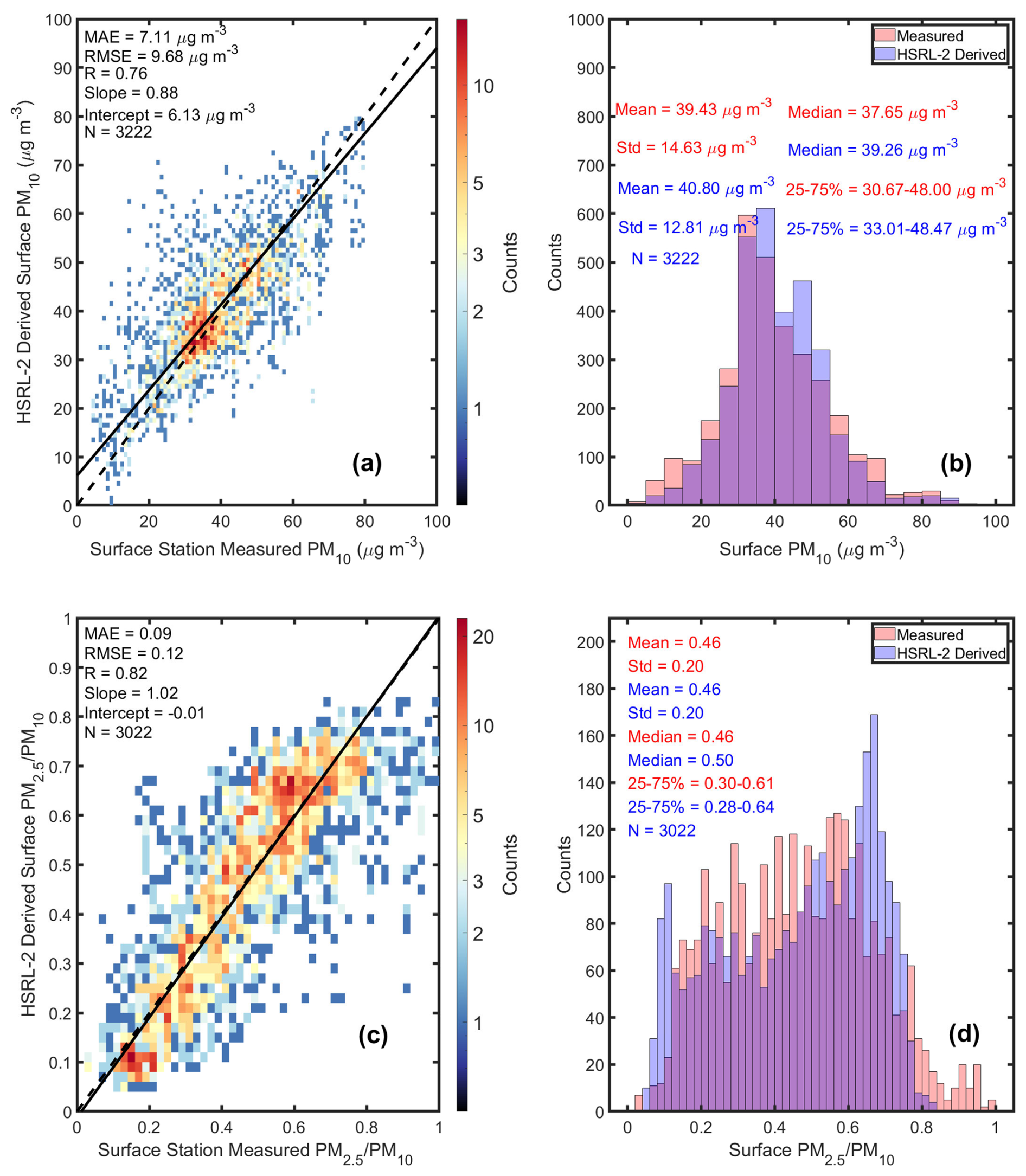
Figure 15 Regression (a) and histogram (b) comparisons of surface PM₁₀ derived from airborne HSRL-2 measurements and measured by surface stations during the NASA ASIA-AQ mission. Panels (c) and (d) are the same except for the ratio PM_2.5 $/$ PM₁₀.

Overall comparisons of HSRL-2 surface PM₁₀ and PM_2.5 $/$ PM₁₀ retrievals and corresponding surface measurements during the ASIA-AQ mission are shown in Fig. 15. These show results when the data from ASIA-AQ were included in the training sets. Consistent with Figs. 5 and 6, retrieval performance for PM₁₀ as indicated by the correlation coefficient and slope is slightly reduced as compared to PM_2.5 (Fig. 15a vs. Fig. 13a). For typical aerosol size distributions, fine mode particles have a greater impact on the HSRL measurements of aerosol optical properties, particularly 355 and 532 nm, than coarse mode particles (Müller and Quenzel, 1985; Veselovskii et al., 2004). Figure 15c and d show that HSRL-2 retrievals of PM_2.5 $/$ PM₁₀ agree well with surface measurements of PM_2.5 $/$ PM₁₀ ratio for most of the range of PM_2.5 $/$ PM₁₀ values with correlation coefficient of 0.82 and slope near unity. HSRL-2 retrievals of PM_2.5 $/$ PM₁₀ ratio do not exceed about 0.85 and so do not capture the small number of high (> 0.8) PM_2.5 $/$ PM₁₀ ratios measured by the ground stations. This is likely due to the small number of such values in the training set used to derive PM_2.5 $/$ PM₁₀ ratio from the HSRL data.

3.4 PM_2.5 and Aerosol Type

Airborne HSRL-2 retrievals of PM_2.5 and inferences of aerosol type provide the means to estimate how various aerosol types contribute to PM_2.5 concentrations. We use a classification algorithm to interpret the information about aerosol physical properties as indicated by the HSRL-2 aerosol intensive parameters. We perform this aerosol type classification empirically using HSRL measurements of aerosol intensive quantities for which the dependence on the aerosol amount has been ratioed out, such as the depolarization ratio (which is a ratio of channels sensitive to different polarizations); lidar ratio (the ratio of the extinction-to-backscatter); or “color ratio” of backscatter (the ratio of backscatter at two different wavelengths, closely related to the Angstrom exponent).

The classification method used here is an update on the method (Burton et al., 2012) which has been used extensively for classification of LaRC airborne HSRL data. The updated version of this algorithm adds the aerosol types “Non-spherical smoke” (Burton et al., 2015) and “Dry maritime” (Ferrare et al., 2023), and it drops the types “Polluted Maritime” and “Fresh Smoke” which subsequent use has shown are often not well separable from other types; it also drops the “Ice” type which was used as a way of filtering observations of fine ice particles observed during a particular Arctic field mission. Information about the aerosol type is embedded in aerosol intensive parameters including the 532 nm lidar ratio and the particulate depolarization at 532 and 1064 nm. In contrast to the original version, the updated algorithm also uses measurements of particulate depolarization and lidar ratio at 355 nm. There are sixteen additional training cases, comprising four each for smoke and pollution cases from both North America and Asia, three dry maritime cases, two each maritime and pure dust cases, and a non-spherical smoke case.

The original methodology was a supervised learning method that used training samples to create four-dimensional Gaussian covariance models of known aerosol types. The distance metric between a multi-dimensional point and multi-dimensional covariance matrix is the Mahalanobis distance, which gives scores or probabilities for the point being associated with the model. The updated classification algorithm uses a combination of this methodology with a decision tree. Specifically, a decision tree with specific thresholds on single variables splits the data into “branches” with one or two aerosol types. Where there are multiple similar aerosol types on a branch, a two-dimensional Gaussian covariance model is used as in the original method (Burton et al., 2012). Limiting the need for covariance models to two types and two variables simplifies the need for training data for each type. An additional advantage of the updated method is that a decision tree avoids non-intuitive mappings of the space such as enclaves. A Gaussian model with large variability in one or more dimensions can act as a sink for noisy observations of all types, even fully surrounding a tighter class that has less variability. A decision tree avoids this problem while also preserving the ability to handle complicated boundaries between similar types in more than one dimension at a time, within the branches of the decision tree.

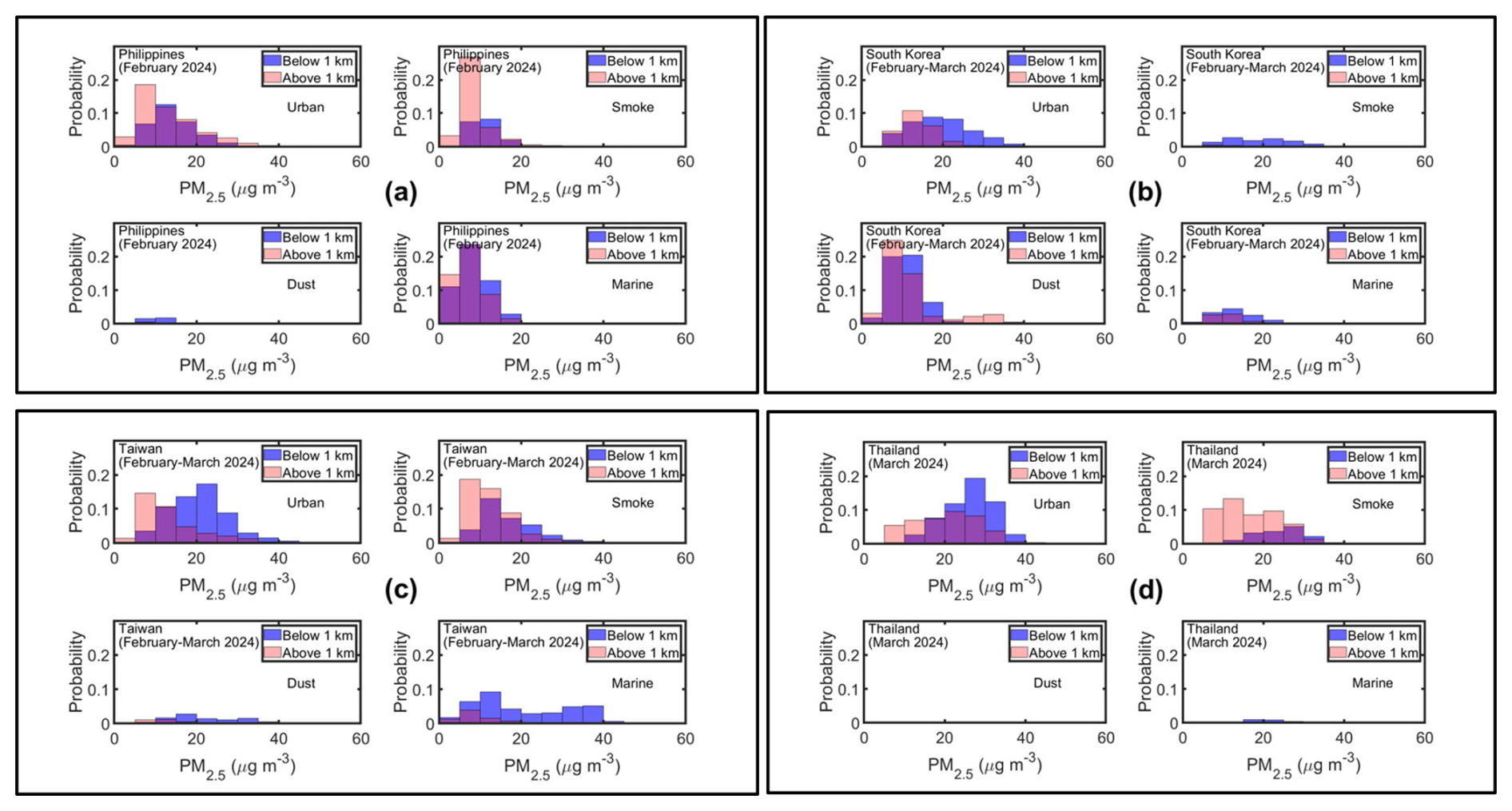
Figure 16 Distribution of PM_2.5 associated with various major aerosol types as identified by the HSRL aerosol classification method for data acquired during the ASIA-AQ campaign. Results are shown for data acquired over the (a) Philippines, (b) South Korea, (c) Taiwan, and (d) Thailand.

Figure 16 shows the distribution of PM_2.5 associated with various major aerosol types (i.e., smoke, urban, dust, marine) as identified by the updated HSRL aerosol classification method for HSRL-2 data acquired during the ASIA-AQ mission. Shown are PM_2.5 values derived during raster patterns over the four main locations of the Asia AQ flights. The results are divided in two altitude regions, 0–1 and 1–4 km, to provide some indication of how the contribution to PM_2.5 by aerosol type varies with altitude. These results show that, excluding South Korea, dust generally contributed little to PM_2.5. Dust has often been observed in lidar measurements over Korea, so it is not surprising that dust is a significant contributor to PM_2.5 in the HSRL-2 retrievals in this location. The optical properties of Asian dust over Korea have been found to vary depending on the altitude of the dust during transport over China. Dust that has crossed highly polluted regions of China at low altitudes are more likely to have been influenced by anthropogenic pollution (Shin et al., 2015).

As PM_2.5 increased over South Korea, urban (pollution) aerosols became more dominant below 1 km. This trend for urban aerosol to be the largest contributor as PM_2.5 increased, particularly below 1 km, is common to all four urban areas. Marine (sea salt) aerosol generally contributes little to PM_2.5 except for the Philippines and, in some cases, over Taiwan. Note that a significant portion of the raster patterns flown by the G-III aircraft during the Philippines portion of ASIA-AQ occurred over Manila Bay. Figure 16d shows that urban aerosol and smoke were the major contributors to PM_2.5 over Bangkok. The HSRL-2 results show that in the lowest kilometer urban aerosol was a larger contributor to PM_2.5 than smoke; in contrast, above 1 km, smoke more often contributed to PM_2.5 except in cases of higher PM_2.5. A somewhat similar pattern was found over Taiwan with urban aerosol the major contributor below 1 km and a combination of smoke and urban aerosol above 1 km.

3.5 Aerosol Type and Mass Extinction Efficiency

The aerosol mass extinction efficiency (MEE) is an important parameter for translating between aerosol optical properties and aerosol mass and, therefore, is crucial for modeling aerosol transport, air quality, and radiative impacts on climate (Kahn, 2012; Kahn et al., 2017; Gliß et al., 2021; Kahn et al., 2023). Because considerable uncertainty exists among models regarding appropriate values associated with different aerosol types (Gliß et al., 2021), various efforts have been proposed to obtain measurements to derive MEE (Kahn et al., 2017). We use HSRL measurements of near surface extinction and retrievals of surface PM_2.5 and PM₁₀ concentrations to obtain estimates of MEE corresponding to the HSRL aerosol types.

An estimate of dry aerosol fine mode MEE, MEE_f, can be obtained from the following equation

$$\begin{array}{}\text{(1)}& \begin{array}{rl}{\mathrm{MEE}}_{\mathrm{f}}& ={\displaystyle \frac{{\mathit{\sigma }}_{\mathrm{a}}}{f\left(\mathrm{RH}\right)\times {\mathrm{PM}}_{\mathrm{2.5}}}}-\left({\displaystyle \frac{{\mathrm{PM}}_{\mathrm{10}}}{{\mathrm{PM}}_{\mathrm{2.5}}}}-\mathrm{1}\right)\times {\mathrm{MEE}}_{\mathrm{c}}\\ & ={\displaystyle \frac{{\mathit{\sigma }}_{\mathrm{a}}}{f\left(\mathrm{RH}\right)\times {\mathrm{PM}}_{\mathrm{2.5}}}}-\left({\displaystyle \frac{\mathrm{1}}{\mathrm{FMF}}}-\mathrm{1}\right)\times {\mathrm{MEE}}_{\mathrm{c}}\end{array}\end{array}$$

where σ_a represents the HSRL near-surface measurement of aerosol extinction (532 nm), PM_2.5 and PM₁₀ represent the near-surface retrievals of PM described earlier, MEE_c represents the mass extinction efficiency of coarse mode aerosols, f(RH) is the humidification factor which represents the increase in scattering associated with hygroscopic growth of hygroscopic aerosols, and FMF is the fine mode fraction. We assume that RH has little impact on aerosol absorption (Nessler et al., 2005; Lynch et al., 2016). The humidification factor is required because HSRL measurements of aerosol extinction are at ambient RH and the derived PM_2.5 concentrations correspond to dry aerosol mass. We use an expression for the humidification factor as given by (Hänel, 1976)

$$\begin{array}{}\text{(2)}& f\left(\mathrm{RH}\right)={\left({\displaystyle \frac{\mathrm{1}-\frac{\mathrm{RH}}{\mathrm{100}}}{\mathrm{1}-({\mathrm{RH}}_{\mathrm{ref}}/\mathrm{100})}}\right)}^{-\mathrm{\Gamma }}\end{array}$$

where RH is the ambient relative humidity from the ERA5 reanalysis, RH_ref is a reference RH set to 30 % (Lynch et al., 2016; Toth et al., 2019), and Γ is a fit parameter assumed to be 0.63, which corresponds to sulfate aerosol (Hänel, 1976; Lynch et al., 2016; Toth et al., 2019). To reduce the impact of f(RH) on estimates of MEE_f, we only examine cases for which RH < 70 %; in such cases f(RH) is less than 1.7 and generally close to unity. We assume that coarse mode aerosol absorption is negligible so that the coarse mode mass extinction efficiency (MEE_c) can be approximated by the coarse mode mass scattering efficiency. Coarse mode mass scattering (extinction) efficiencies typically range from roughly 0.5 to 1.5 m² g⁻¹ (Hand and Malm, 2007; Jung et al., 2018) so we have computed MEE_f assuming that MEE_c can vary over this range. To reduce the dependence of the estimated MEE_f on MEE_c, we avoid cases for which coarse mode aerosol extinction dominates and so examine cases for which the fine mode fraction (FMF) = PM_2.5 $/$ PM₁₀ is greater than 0.5.

We examine cases corresponding to four major aerosol types identified by the HSRL aerosol classification algorithm during the ASIA-AQ mission: dusty mix, maritime, urban, and smoke. Figure 17 shows the retrieved MEE_f for these four types. The median value for dusty mix (3.3 m² g⁻¹) is within the range of mass scattering efficiency (2.6–3.4 m² g⁻¹) reported for fine mode dust (Hand and Malm, 2007). The median value for maritime aerosol (2.6 m² g⁻¹) is lower than the value associated with fine mode sea salt (4.5 m² g⁻¹) (Hand and Malm, 2007); however, this study recommends a much lower value (∼ 1.2 m² g⁻¹) if some coarse mode sea salt aerosol is included in the sampling. The median value for urban aerosol (3.8 m² g⁻¹) is close to the value of 3.4 m² g⁻¹ used for pollution aerosol over the US (Toth et al., 2019, 2022), the value of 3.6 m² g⁻¹ recommended for mixed fine mode aerosol (Hand and Malm, 2007), and the value of 4.4 ± 0.8 m² g⁻¹ found for urban China (Cheng et al., 2017). The median value of 5.0 m² g⁻¹ for smoke falls at the upper range of smoke MEE (1.5 to 6 m² g⁻¹) (Saide et al., 2022) reported from laboratory and field measurements and most likely corresponds to aged smoke (Reid et al., 2005; Kleinman et al., 2020; Saide et al., 2022).

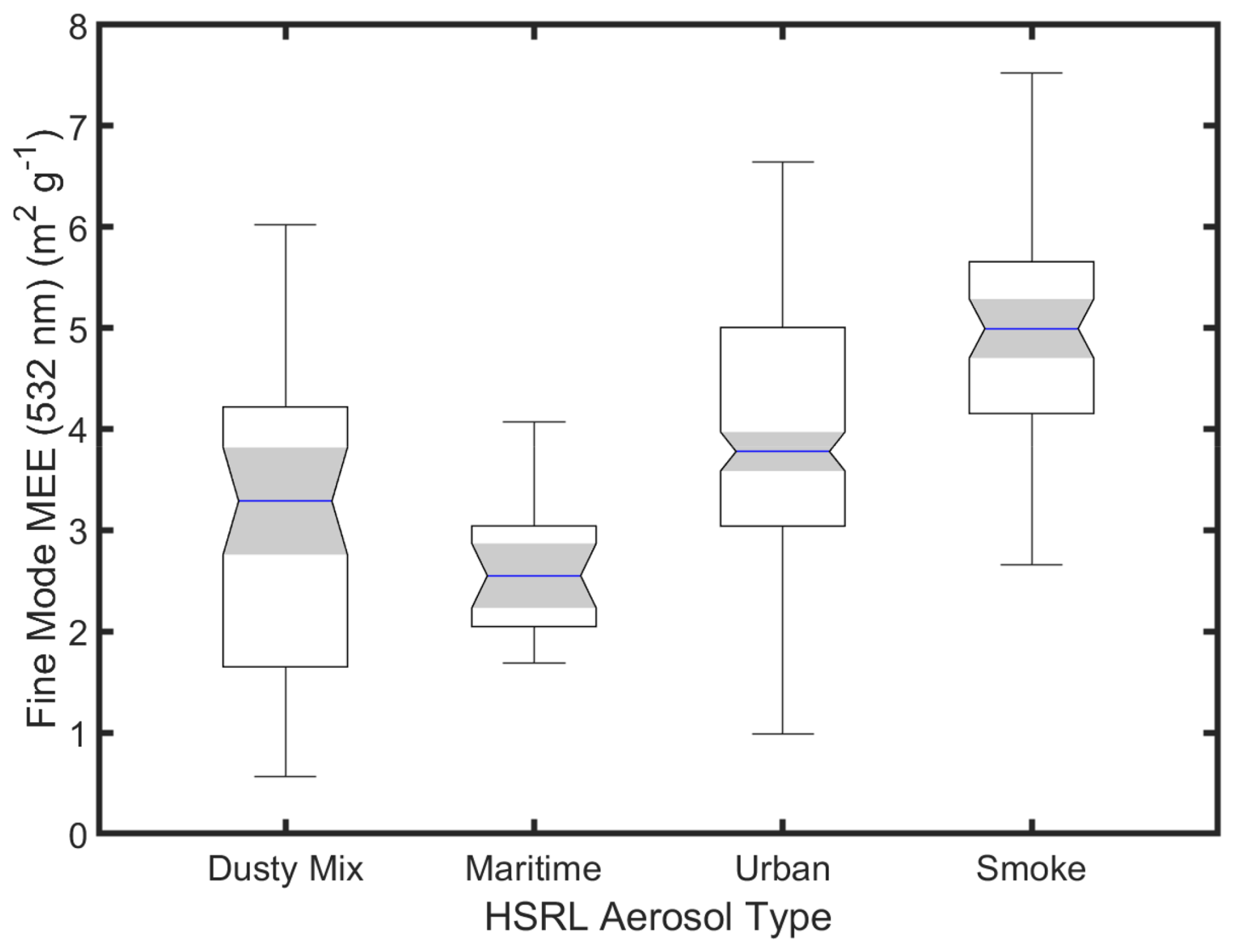
Figure 17 Box chart showing the MEE_f retrieved from the HSRL-2 measurements for data acquired during the ASIA-AQ mission. The results are shown for the various major aerosol types as identified by the HSRL aerosol classification method. Blue lines inside each box correspond to the median. Top and bottom edges of each box are the upper and lower quartiles, respectively. Whiskers represent the maximum and minimum values. Boxes whose shaded notch regions do not overlap have different medians at the 5 % confidence level.

We also compare MEE_f derived from the HSRL-2 data and from the DC-8 in situ data like the PM_2.5 comparison shown in Fig. 14. Recall that DC-8 MEE_f is derived using the submicrometer dry aerosol extinction and PM_2.5 derived from the DC-8 in situ measurements. As discussed above, to reduce the impact of uncertainties in f(RH) and MEE_c, we compare HSRL-2 retrievals of MEE_f for which RH < 70 % and FMF > 0.5. Figure 18 shows that MEE_f derived from the HSRL-2 and DC-8 are in generally good agreement with MAE and RMS differences less than 1 m² g⁻¹. In addition, both retrievals show the tendency of MEE_f to increase as the aerosol type changed from maritime to urban to smoke. Some of the discrepancies can be explained by the large variability in the 1 min averages, which likely represents inhomogeneous conditions with large gradients in aerosol properties.

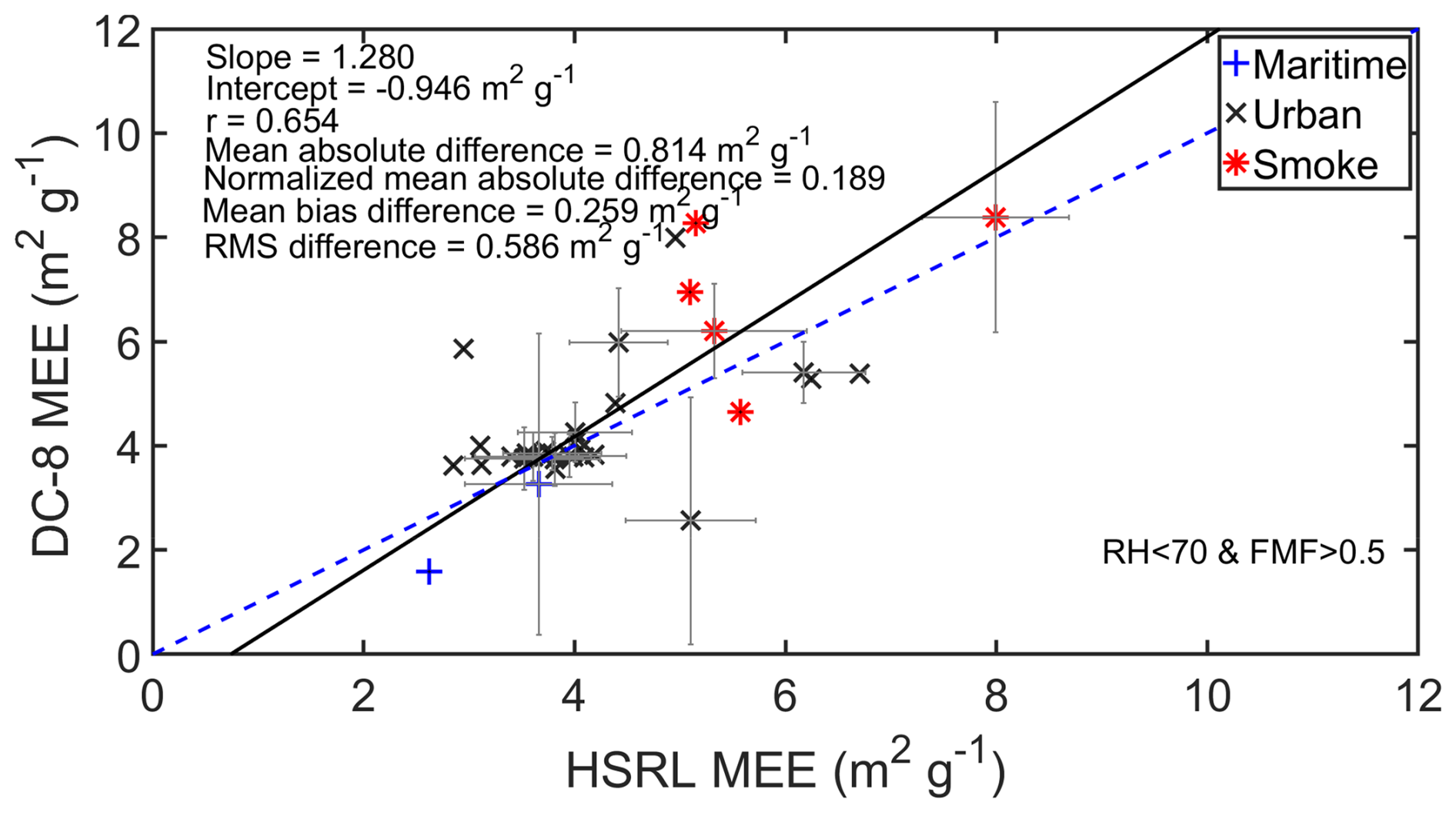
Figure 18 Comparison of MEE_f derived from HSRL-2 data (x axis) vs. MEE_f derived from DC-8 in situ instruments (y axis) during the ASIA-AQ mission. Results are color-coded by aerosol type inferred from HSRL-2 data. The solid line represents a least-squares bisector fit and the dashed line represents the 1 : 1 line. Error bars represent the two standard deviations derived from the 1 min averages.

4 Summary and Conclusion

We have developed a new method to retrieve PM_2.5 and PM₁₀ concentrations using airborne High Spectral Resolution Lidar (HSRL) measurements in machine learning regression algorithms. Unlike previous methods that have used airborne HSRL data to derive surface PM_2.5 concentrations, this method does not require the HSRL qualitative inferences of aerosol type or aerosol chemical composition information provided by models. Nor does this method require estimates or assumptions of the mass extinction efficiency, aerosol humidification factor, fine mode fraction, or particle density. This method takes advantage of the extensive set of airborne HSRL measurements acquired over major metropolitan regions in the United States and Asia over many years. We use hourly surface PM_2.5 and PM₁₀ measurements acquired within 10 km and 15 min of these near-surface HSRL measurements to train models that compute PM concentrations based on these HSRL measurements. The extensive airborne HSRL datasets of aerosol measurements over metropolitan areas and surface are particularly well suited for developing this methodology of inferring surface PM concentrations. These algorithms take advantage of the unique capability of airborne HSRL systems to provide accurate aerosol measurements near the surface. In contrast to backscatter lidars, these systems provide direct measurements of near-surface calibrated aerosol backscatter and aerosol extinction without additional constraints or assumptions to account for attenuation by overlying aerosols. Also, HSRL systems provide measurements of aerosol intensive properties that provide valuable information regarding aerosol shape, size, and composition to help account for variations in these aerosol properties.

Our investigations have focused on the use of the aerosol properties (aerosol backscatter, extinction, depolarization) that are measured by these lidars and, except for relative humidity, have not attempted to include additional meteorological, surface, or aerosol parameters in these model regressions. There are three reasons for this. First, focusing on regression models that exclusively use airborne HSRL measurements provides the ability to retrieve accurate estimates of PM concentrations using HSRL measurements in near real-time when measurements or model simulations of additional meteorological and/or aerosol parameters are often unavailable. This permits rapid use of these PM retrievals to assess model forecasts and rapidly changing conditions over urban areas which is particularly useful in planning and executing field missions designed to study air quality. Second, these retrievals are independent of model simulations and model parameters and so represent an unbiased method to evaluate the model results. Third, the HSRL measurements themselves contain key information regarding aerosol shape, size, and composition and have been used in various methodologies to retrieve these parameters. Therefore, including such measurements in the machine learning regression provides the ability of these ML models to capture changes in aerosol type and physical properties (size, shape, composition) such as those caused by changes in relative humidity that impact the ability to infer PM concentrations. We found surface relative humidity to have minimal impact on the retrievals of surface PM and believe this is due, at least in part, to the inclusion of HSRL measurements of aerosol intensive parameters that respond to changes in RH.

We examined several regression methods and found that exponential Gaussian Process regression (GPR) algorithms consistently give the best retrieval performance in terms of the lowest root-mean-square (RMS) errors and the highest correlations. These GPR models also have the advantage of providing uncertainty estimates to quantify the confidence in the predictions. A disadvantage of GPR models is that such models can be computationally expensive. We also tested several different combinations of airborne HSRL measurements of near-surface aerosol parameters (e.g., aerosol backscatter, extinction, depolarization, backscatter color ratios, lidar ratios, aerosol optical thickness) and retrievals (e.g., mixed layer height, aerosol type) used in the ML regressions. Models that use near-surface measurements of aerosol backscatter and aerosol intensive properties such as depolarization, backscatter color ratio, and lidar ratio yielded retrievals of surface PM_2.5 that agreed well with surface PM measurements; RMS differences between HSRL retrievals and surface PM_2.5 measurements were around 5 µg m⁻³ with correlation coefficients above 0.8. Model performance was generally better for models that used near-surface aerosol backscatter rather than near-surface aerosol extinction. This is because near-surface aerosol backscatter profile measurements extend closer to the surface (within ∼ 60–100 m) than near-surface aerosol extinction profiles (within ∼ 200–350 m). Also, the HSRL measurements of aerosol backscatter have smaller uncertainties and so are less noisy than the aerosol extinction measurements. Corresponding results for PM₁₀ were slightly worse, with RMS differences around 11 µg m⁻³ and correlation coefficients around 0.7. These comparison results were derived using data withheld from the training sets. Shapley scores reveal that aerosol backscatter (532 nm) was by far the most important variable for retrieving surface PM_2.5, and to a lesser extent, surface PM₁₀. Aerosol depolarization (532 nm) was the most important parameter for retrieving estimates of the PM_2.5 $/$ PM₁₀ ratio due to its sensitivity to coarse mode nonspherical dust particles.

We used the airborne HSRL-2 aerosol measurements acquired during the recently completed NASA ASIA-AQ campaign to derive qualitative estimates of aerosol types using an updated aerosol classification algorithm. This new algorithm differs from our previous algorithm in two ways. First, it uses aerosol measurements acquired at 355 nm in additional to measurements acquired at 532 and 1064 nm. Second, the updated algorithm uses a decision tree in addition to the Mahalanobis distance metric. The PM_2.5 retrievals showed that dust contributed little to the PM_2.5 concentrations over the Philippines, Taiwan, and Thailand but had larger contributions over South Korea. For all areas, urban aerosol type became the largest contributor as PM_2.5 levels increased. Over Thailand, both smoke and urban area were large contributors, with smoke providing the largest contribution above 1 km.

We used these estimates of aerosol types along with HSRL measurements of aerosol extinction and retrievals of surface PM_2.5 to derive estimates of fine mode mass extinction efficiency MEE_f associated with major aerosol types. These estimates correspond to conditions of lower RH (< 70 %) and where the ratio PM_2.5 $/$ PM₁₀ is above 0.5. MEE_f values for dusty mix (3.3 m² g⁻¹) and urban aerosol (3.8 m² g⁻¹) fall with the ranges reported elsewhere. The median value for smoke (5.0 m² g⁻¹) lies at the upper range of reported values and most likely corresponds to aged smoke. The HSRL-2 PM_2.5 retrievals and MEE_f estimates are consistent with those derived from airborne in situ estimates.

The ML methodology described here can also be applied to ground-based and space-based lidars. For the former, it probably would be best to use a single training set based on measurements from several locations to include a wide variety of different aerosol types with different levels of PM. This training set could be developed using measurements from several of these lidars assuming that coincident and collocated measurements of PM were available for training. It would also be beneficial that measurements from these lidars had the same or very similar temporal and vertical resolutions and averaging characteristics.

In the case of the space-based lidars, satellite aerosol measurements such as those from the ATLID sensor on board the EarthCARE satellite could also be used with this ML methodology. ATLID is also an HSRL and so it independently measures backscattered light from atmospheric aerosols and backscattered light from atmospheric molecules, which enables it to derive independently both aerosol backscatter and extinction. Our tests using airborne HSRL-2 data using data only acquired at 355 nm showed retrieval performance comparable to that obtained using data from two (532 and 1064 nm) and three wavelengths (355, 532, 1064 nm). Since ATLID also provides measurements of aerosol extinction, backscattering, and depolarization at 355 nm, these three parameters could be used in the same regression model that was developed using the corresponding airborne HSRL-2 data. Alternatively, a separate machine learning regression algorithm could be developed using these ATLID measured aerosol parameters trained using coincident hourly measurements of surface PM_2.5 from EPA surface stations and from similar networks in other countries. Carefully chosen training data sets that include a wider range of PM values, locations, and aerosol parameters acquired during both daytime and nighttime could be used to construct a robust regression model. Such a model could take advantage of global data and so would have the advantage of being applicable over a much wider range of PM values.

Long-term satellite lidar measurements such as those from ATLID offer the opportunity to provide a unique long-term global lidar record of near-surface aerosol measurements that can be leveraged to study temporal and spatial variations in PM. For example, twelve years of CALIOP measurements of near-surface aerosol extinction were used to derive multi-year mean and trends of surface PM_2.5 over the contiguous United States (Toth et al., 2022). ATLID measurements provide the means to extend this record. These satellite and airborne HSRL measurements described here can be used to evaluate the ability of aerosol models to depict the vertical structure of aerosols, apportion aerosol extinction and optical thickness to aerosol species, and estimate PM concentrations.