Benchmarking K_DP in rainfall: a quantitative assessment of estimation algorithms using C-band weather radar observations

Accurate and precise K_DP estimates are essential for radar-based applications, especially in quantitative precipitation estimation and radar data quality control routines. The accuracy of these estimates largely depends on the post-processing of the radar's measured Φ_DP, which aims to reduce noise and backscattering effects while preserving fine-scale precipitation features. In this study, we evaluate the performance of several publicly available K_DP estimation methods implemented in open-source libraries such as Py-ART (the Python ARM (atmospheric radiation measurement) Radar Toolkit) and ωradlib and the method used in the Vaisala weather radars. To benchmark these methods, we employ a polarimetric self-consistency approach that relates K_DP to reflectivity and differential reflectivity in rain, providing a reference self-consistent K_DP ($K_{\mathrm{DP}}^{\mathrm{sc}}$) for comparison. This approach allows for the construction of the reference K_DP observations that can be used to assess the accuracy and robustness of the studied K_DP estimation methods. We assess each method by quantifying uncertainties using C-band weather radar observations, where the reflectivity values ranged between 20 and 50 dBZ.

Using the proposed evaluation framework, we were able to define optimized parameter settings for the methods that have user-configurable parameters. Most of these methods showed a significant reduction in the estimation errors after the optimization, with respect to the default settings. We have found significant differences in the performance of the studied methods, where the best-performing methods showed smaller normalized biases in the high reflectivity values (i.e., ≥ 40 dBZ) and overall smaller normalized root-mean-square errors across the range of reflectivity values.

1 Introduction

The specific differential phase (K_DP) plays an important role in many weather radar applications, particularly in hydrometeor classification (Höller et al., 1994; Vivekanandan et al., 1999; Liu and Chandrasekar, 2000; Zrnić et al., 2001; Keenan, 2003; Lim et al., 2005; Tessendorf et al., 2005; Marzano et al., 2007; Dolan and Rutledge, 2009; Park et al., 2009; Snyder et al., 2010; Al-Sakka et al., 2013; Dolan et al., 2013; Thompson et al., 2014; Bechini and Chandrasekar, 2015; Grazioli et al., 2015; Wen et al., 2015; Besic et al., 2016; Ribaud et al., 2019) and quantitative precipitation estimation (QPE) (Sachidananda and Zrnić, 1987; Chandrasekar et al., 1990; Ryzhkov and Zrnić, 1995, 1996; May et al., 1999; Bringi and Chandrasekar, 2001; Bringi et al., 2006; Matrosov et al., 2006; Giangrande and Ryzhkov, 2008; Bringi et al., 2011; Cifelli et al., 2011; Wang et al., 2013; Figueras i Ventura and Tabary, 2013; Chen and Chandrasekar, 2015; Chen et al., 2017; Thompson et al., 2018; Zhang et al., 2020), and is used in data assimilation for numerical weather prediction models (Thomas et al., 2020; Du et al., 2021) and in hydrological applications (Brandes et al., 2002; Ryzhkov et al., 2005a; Vulpiani et al., 2012; Li et al., 2023; Cremonini et al., 2023). Compared to radar power variables; i.e., the reflectivity factor at horizontal polarization (Z_H) and differential reflectivity (Z_dr), K_DP offers advantages in terms of accuracy, resilience, and reliability due to its immunity to radar miscalibration, attenuation (Bringi and Chandrasekar, 2001; Illingworth, 2004; Ryzhkov and Zrnic, 2019), and partial beam blockage (Zrnić and Ryzhkov, 1996). It has also proven successful in hydrometeor classification routines (Lim et al., 2005; Park et al., 2009; Grazioli et al., 2015; Tiira and Moisseev, 2020), especially in the detection of graupel (Dolan and Rutledge, 2009; Oue et al., 2015) and small melting hail (Kumjian et al., 2019), and in the dendritic growth zone and the processes within (Kennedy and Rutledge, 2011; Andrić et al., 2013; Schneebeli et al., 2013; Moisseev et al., 2015; Kumjian and Lombardo, 2017). The ability of K_DP to accurately estimate heavy rainfall, differentiate hydrometeor types, and overcome attenuation in precipitation makes it an invaluable operational and research radar variable.

Despite its advantages, accurate estimation of K_DP from the radar-measured differential phase (Φ_DP) remains challenging. Mathematically, K_DP is half of the range derivative of Φ_DP, which measures the phase shift between horizontally and vertically polarized signals as they propagate through precipitation. This phase shift (Φ_DP) is influenced by hydrometeor concentration, shape, orientation, and composition (Kumjian, 2018). However, Φ_DP is not typically smooth and does not monotonically increase along the rain path; it contains fluctuations due to noise (ϵ) and the backscattering differential phase (δ_HV) (Ryzhkov and Zrnić, 1996; Ryzhkov and Zrnic, 1998). Excessive filtering of Φ_DP to remove ϵ can lead to the loss of fine-scale precipitation features, affecting the accuracy of K_DP estimates, especially in light precipitation (Huang et al., 2017). In heavier precipitation, δ_HV causes spikes in Φ_DP, especially at higher radar frequencies, further complicating accurate K_DP estimation (Bringi and Chandrasekar, 2001).

To address these challenges, various methods have been developed to post-process Φ_DP and derive K_DP (Hubbert et al., 1993; Hubbert and Bringi, 1995; Ryzhkov et al., 2005c; Wang and Chandrasekar, 2009; Otto and Russchenberg, 2011; Maesaka et al., 2012; Vulpiani et al., 2012; Schneebeli and Berne, 2012; Giangrande et al., 2013; Schneebeli et al., 2014; Huang et al., 2017; Reinoso-Rondinel et al., 2018; Wen et al., 2019). Basic approaches include median filters and moving windows, while more advanced methods use regression techniques and self-consistency constraints based on Z_H or Z_dr. Many of these methods are now available in open-source Python libraries such as the Python ARM (atmospheric radiation measurement) Radar Toolkit (Py-ART; Helmus and Collis, 2016) and ωradlib (Heistermann et al., 2013). For this study, some of the most popular methods based on Maesaka et al. (2012), Vulpiani et al. (2012), Giangrande et al. (2013), and Schneebeli et al. (2014) were selected for analysis. Additionally, the K_DP product implemented by Vaisala in the IRIS software (Vaisala, 2017), based on Wang and Chandrasekar (2009), was also included in our analysis. Each algorithm has its own data requirements, mathematical approach, and optimizing parameters, raising the question of which method performs optimally under varying parameter settings and rainfall intensities.

Recent studies show that K_DP estimates can vary significantly depending on the algorithm and the optimizing parameters used. Reimel and Kumjian (2021) evaluated the errors in several methods using synthetic K_DP profiles and found that no single algorithm was optimal across all rainfall conditions. Instead, performance varied according to the complexity of the rain profile and the parameters selected. They identified kdp_maesaka (Py-ART's implementation of the Maesaka et al., 2012, method) and phase_proc_lp (Py-ART's implementation of the Giangrande et al., 2013, method) as particularly versatile. However, Reimel and Kumjian (2021) used synthetic data, which may miss some of the effects present in radar observations of rainfall (e.g., δ_HV). More recently, Li et al. (2023) compared kdp_maesaka and phase_proc_lp in an extreme summer rainfall event, finding that fine-tuning the methods played a key role in retrieving the most accurate K_DP estimate. Despite these insights, the performance of and uncertainties in most methods of rainfall observations remain largely unexplored.

The goal of this study is to evaluate the performance of publicly available K_DP estimation methods on real rainfall observations and quantify their uncertainties as a function of reflectivity intensities. To achieve this, we employ a benchmarking K_DP, herein $K_{\mathrm{DP}}^{\mathrm{sc}}$, computed from measured Z_H and Z_dr, and use self-consistency relations in rain. In rainfall observations, the polarimetric radar variables are not independent, but one can be computed in terms of the others via the self-consistency relations (Aydin et al., 1987; Scarchilli et al., 1993). These relations have proven successful in hydrometeor classification (Aydin and Giridhar, 1992) and radar calibration correction (Gorgucci et al., 1992) routines. For instance, Aydin and Giridhar (1992) showed that the hydrometeors can be classified based on their proximity to clusters around self-consistency curves between polarimetric variables. At nearly the same time, Gorgucci et al. (1992) noted the self-consistency of Z_H, Z_dr, and K_DP in rainfall and proposed a method to calibrate Z_H and correct Z_H–rainfall estimates, benchmarking against K_DP–rainfall estimates. Thereafter, several methods linking the polarimetric variables via self-consistency relations have been widely used to calibrate Z_H (Goddard et al., 1994; Scarchilli et al., 1996; Vivekanandan et al., 2003; Ryzhkov et al., 2005b; Gourley et al., 2009). In this study, $K_{\mathrm{DP}}^{\mathrm{sc}}$ is computed using the consistency relation linking K_DP to Z_H and Z_dr, which was first noted by Goddard et al. (1994) and described in Gourley et al. (2009), requiring thorough selection and filtering of Z_H and Z_dr. $K_{\mathrm{DP}}^{\mathrm{sc}}$ computed from quality controlled Z_H and Z_dr measurements provides a solid benchmark against which to compare the methods' performance, to select optimal parameters, and to quantify the associated uncertainties.

This paper is organized as follows. Section 2 describes the radar and disdrometer data, shows the evaluation framework, and introduces the K_DP estimation methods. Section 3 presents and discusses the parameter optimization and performance evaluation of the methods, and Sect. 4 summarizes the findings.

2 Data and methods

2.1 Radar and disdrometer data

This study evaluates the performance of K_DP estimation methods using real rainfall data. The dataset was collected from the Finnish Meteorological Institute (FMI) C-band Vantaa radar, located near Helsinki, Finland (see Fig. 1). The radar recorded various quantities, including Z_H, Z_dr, Φ_DP, K_DP, the cross-correlation coefficient (ρ_HV), and the hydrometeor classification product available in IRIS (Vaisala, 2017) and based on the methodology described by Chandrasekar et al. (2013). The spatial resolution of the radar is 500 m in range and 1° in azimuth, with scans performed every 5 min, and the data were collected with an elevation angle of 0.7°. The dataset spans June to September during the years 2017 to 2019, capturing precipitation events with variable rainfall intensities and spatial extents. The raw radar dataset as well as the post-processed K_DP estimates are available from the link provided in Aldana (2024).

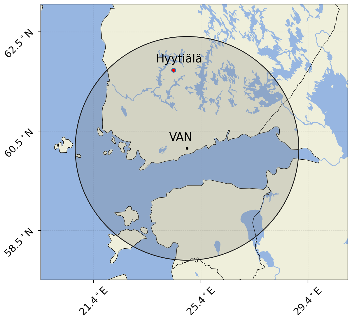
Figure 1 Map showing the locations of FMI's Vantaa radar (VAN) and Hyytiälä's research station where the drop size distribution (DSD) data were collected. The shaded area is a circle with a 250 km radius corresponding to the spatial coverage of the radar.

To ensure data quality, only periods when the Vantaa radar had calibration errors within 1 dB were selected. The calibration was verified by (i) identifying periods where solar flux estimates from Vantaa radar estimates aligned consistently with Dominion Radio Astrophysical Observatory (DRAO) estimates (Huuskonen and Holleman, 2007; Tapping, 2013; Holleman et al., 2022) and (ii) selecting radar scans within the periods where Z_H-calibration offsets were within 1 dB, following the absolute calibration procedure outlined by Gourley et al. (2009). Z_dr bias was estimated and corrected during these periods by computing the offset between observed and self-consistent Z_dr derived from observed Z_H, as described in Hickman (2015), and by computing the average for several cases.

The performance of the K_DP estimation methods is benchmarked against the self-consistent $K_{\mathrm{DP}}^{\mathrm{sc}}$ computed from measured Z_H and Z_dr and by using self-consistency relations in rain. The self-consistency relations, which link the polarimetric radar variables, were derived by fitting radar variables computed using the open-source library, PyTMatrix (Leinonen, 2014). PyTMatrix provides a simple interface for T-matrix electromagnetic scattering calculations (Waterman, 1965; Mishchenko et al., 2000), requiring the user to provide drop size distribution (DSD) data and setting parameters such as temperature, the radar wavelength band, and the raindrop shape model. The parameters used for the T-matrix calculations were 10 °C, C-band, and Thurai et al. (2007), respectively, and the DSD data provided were collected by an optical Parsivel disdrometer (Moisseev, 2024) located in Hyytiälä, Finland (see Fig. 1).

The Parsivel disdrometer records the number of particles and their velocity at 1 min intervals, sorting the data into 32 bins depending on the particle's size (i.e., equivalent volume diameter) and 32 additional bins depending on the particle's fall velocity. From the number of particles and the size and velocity classes, the Parsivel disdrometer computes the precipitation type, which was used to filter out non-liquid particles. Observations were further limited to times when the 30 min average 2 m temperature exceeded 2 °C to ensure liquid rain. Following the filtering procedure suggested by Leinonen et al. (2012) to reduce statistical errors, only those measurements with at least 100 counts in two consecutive bins and positive counts in at least four consecutive bins were retained. The disdrometer dataset, covering June to September from 2014 to 2019, provided a robust basis for deriving average summer-season DSD parameters such as the mean volume diameter (D₀) and intercept (N_w) and shape (μ) parameters. These parameters showed strong agreement with those reported by Leinonen et al. (2012) in a climatological study of Finland. From the derived DSD parameters (N_w, D₀, and μ), the polarimetric radar variables were computed and used to derive the self-consistency relation, defining the framework to evaluate the K_DP estimation methods.

2.2 K_DP evaluation framework

The performance of the K_DP estimation methods is evaluated using $K_{\mathrm{DP}}^{\mathrm{sc}}$ as a benchmark. This quantity is calculated from each radar-measured tuple (Z_H, Z_dr), following a relationship of the form (Goddard et al., 1994; Illingworth and Blackman, 2002; Gourley et al., 2009)

$$\begin{array}{}\text{(1)}& K_{\mathrm{DP}}^{\mathrm{sc}}=z_{\mathrm{H}}\times {\mathrm{10}}^{-\mathrm{5}}\times \left(a_{\mathrm{1}}+a_{\mathrm{2}}\times Z_{\mathrm{dr}}+a_{\mathrm{3}}\times Z_{\mathrm{dr}}^{\mathrm{2}}+a_{\mathrm{4}}\times Z_{\mathrm{dr}}^{\mathrm{3}}\right),\end{array}$$

where $z_{\mathrm{H}}={\mathrm{10}}^{\mathrm{0.1}\times Z_{\mathrm{H}}}$ represents Z_H in linear units (mm⁶ m⁻³), and Z_dr is in decibels (dB). The coefficients used in this relation are a₁=6.78, $a_{\mathrm{2}}=-\mathrm{2.65}$, a₃=0.562, and $a_{\mathrm{4}}=-\mathrm{0.0624}$. The coefficients align well with those reported by Gourley et al. (2009), which employed the raindrop shape models by Brandes et al. (2002) and Thurai and Bringi (2005).

To ensure the accuracy and robustness of the $K_{\mathrm{DP}}^{\mathrm{sc}}$ estimates used in the method assessment, it was crucial to quality control the Z_H and Z_dr data. Radar observations of rain are often affected by non-meteorological measurements, resonance effects, and hail contamination (Bringi and Chandrasekar, 2001; Kumjian, 2013; Ryzhkov and Zrnic, 2019). To address these issues, the following filtering steps were applied.

• Noise filtering. A minimum threshold of 0.97 was applied to ρ_HV.

• Non-meteorological observation filtering. The hydrometeor classification product from IRIS (Vaisala, 2017), based on Chandrasekar et al. (2013), was used to exclude gates classified as non-meteorological.

• δ_HV reduction. Gates with Z_dr > 3.5 dB were excluded (Bringi and Chandrasekar, 2001; Gourley et al., 2009).

• Non-liquid rain filtering.

  • Only radar scans from the warm months (June–September) were selected.

  • Gates not classified as rain by the hydrometeor classification product were excluded.

  • Hail contamination was addressed by removing gates with Z_H ≥ 50 dBZ.

  • Observations from the melting layer and above were suppressed by masking gates further than 70 km (see last dashed ring in Fig. 2) from the radar in the radial direction. The distance was manually set by identifying gates with melting layer signatures (Giangrande et al., 2008; Boodoo et al., 2010).

In addition to addressing noise and non-liquid rain measurements, $K_{\mathrm{DP}}^{\mathrm{sc}}$ estimates are affected by attenuation in Z_H and differential attenuation in Z_dr, particularly in cases of heavy rainfall, of extended propagation paths through rain (hereafter rain paths) (Zrnić and Ryzhkov, 1996; Carey et al., 2000; Bringi and Chandrasekar, 2001; Kumjian, 2013), and when the radar's antenna radome is wet (Blevis, 1965; Kurri and Huuskonen, 2008). To mitigate these effects, radar scans when there was rain on top of the radar within the past 20 min were discarded. Then, for the remaining cases, attenuation in heavy precipitation or extended rain paths was addressed by flagging the radar gates when suspected attenuation of at least 1 dB was detected. The attenuation in range gates was inferred using a standard method that linearly relates the losses in Z_H and Z_dr to increases in ΔΦ_DP (Ryzhkov and Zrnić, 1995; Carey et al., 2000; Bringi and Chandrasekar, 2001; Gourley et al., 2009). ΔΦ_DP corresponds to the total span of Φ_DP along the radial within a rain path. A rain path was defined as a set of consecutive gates with rain features extending at least 20 km in the radial direction. For C-band radar, a minimum threshold of 12° in ΔΦ_DP indicates attenuation of at least 1 dB (Carey et al., 2000). In this study, a threshold of 10° was used, meaning that gates within rain paths featuring ΔΦ_DP ≥ 10° were flagged as attenuated.

An example of the filtering procedure applied to a radar scan is shown in Fig. 2. This figure demonstrates the effects of the filtering process and the attenuation considered on the chosen data samples.

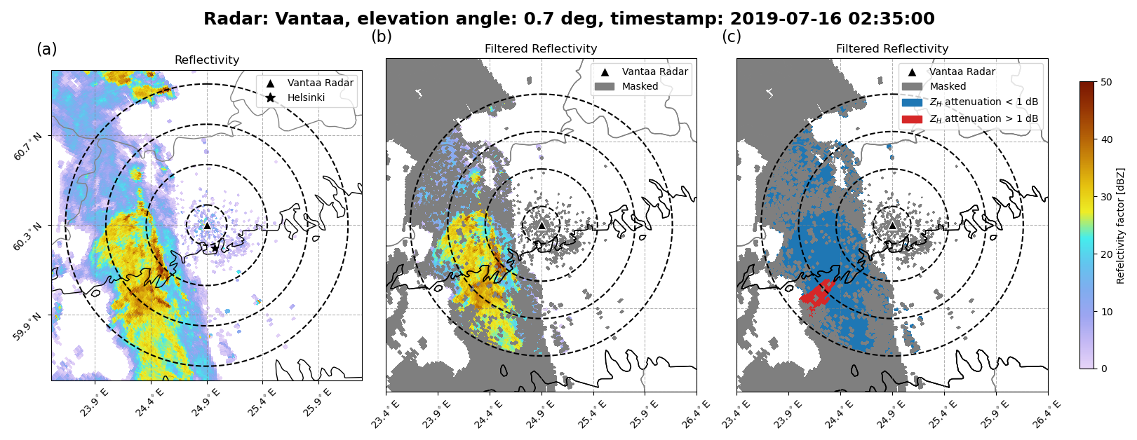
Figure 2 Example of a Vantaa radar scan during a precipitation event on 16 July 2019 at an elevation angle of 0.7°. Panel (a) shows measured Z_H; panel (b) shows filtered Z_H with masked gates in gray; panel (c) shows the same as panel (b) but with attenuated gates marked in red and non-attenuated gates marked in blue. Dashed rings represent radial distances of 10, 30, 50, and 70 km from the radar.

Following the filtering process, the dataset comprised 652 624 quality controlled gates from 70 radar scans. Figure 3 presents a histogram of the data proportions across different Z_H values, showing the highest percentage of data between 30 and 35 dBZ, with a sharp decrease from 35 to 50 dBZ. The stacked bars indicate the percentages of attenuated and non-attenuated gates, with the ratio of attenuated to non-attenuated data increasing with greater Z_H.

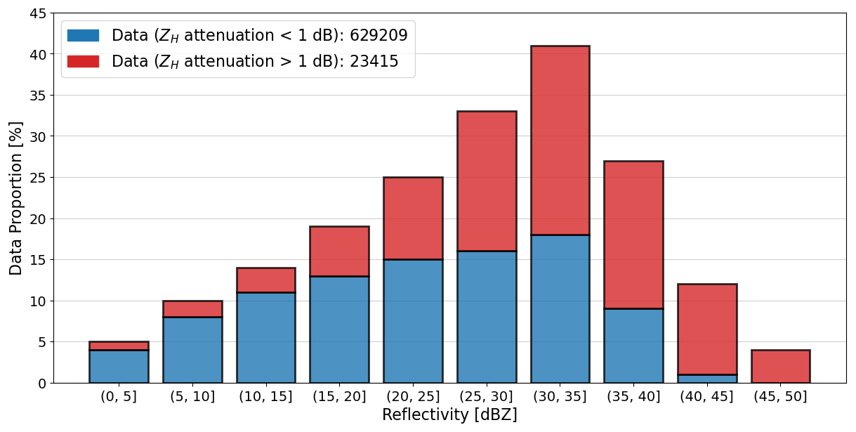
Figure 3 Proportion of data across Z_H intervals of 5 dBZ. Attenuated data are represented by red bars, and non-attenuated data are represented by blue bars. The legend indicates the total number of gates with suspected attenuation of at least 1 dB (red) and less than 1 dB (blue).

2.3 K_DP estimation methods

This section provides an overview of the K_DP estimation methods selected for this study. The selection criteria focused on the availability of these methods in widely used open-source libraries, such as Py-ART (Helmus and Collis, 2016) and ωradlib (Heistermann et al., 2013). At the time of this study, Py-ART version 1.17.0 included the following methods: kdp_maesaka, kdp_vulpiani, phase_proc_lp, and kdp_schneebeli. ωradlib version 2.0.3 included kdp_from_phidp and phidp_kdp_vulpiani. However, phidp_kdp_vulpiani was excluded from our analysis, as it is based on the same method proposed by Vulpiani et al. (2012) that is already represented in Py-ART by kdp_vulpiani. Additionally, kdp_iris, a method based on Wang and Chandrasekar (2009) and implemented by Vaisala in the IRIS software (Vaisala, 2017), was included. Table 1 summarizes the key features of the selected methods, and a brief description of the methods is provided below.

• a.

  kdp_maesaka. Developed by Maesaka et al. (2012) and available in Py-ART, this method estimates non-negative K_DP from liquid-precipitation measurements. It addresses the issue of negative K_DP estimates observed in exclusively liquid-precipitation regions when using classical methods based on iterative filtering and local linear regression. Maesaka et al. (2012) identified that negative K_DP were caused by noise in Φ_DP during weak precipitation and by δ_HV during heavy precipitation. The method restricts K_DP to positive values and assumes that Φ_DP is a monotonically increasing function with range, which is already unfolded.

• b.

  kdp_vulpiani. Developed by Vulpiani et al. (2012) and available in Py-ART, this method estimates K_DP for any type of precipitation. It uses a multistep moving-window range derivative approach to obtain K_DP. It calculates a K_DP profile from the range derivative of a noise-reduced, offset-corrected, and unfolded Φ_DP profile. At each window, K_DP is compared to thresholds representing unrealistic K_DP values within precipitation, correcting possible aliasing with the minimum threshold.

• c.

  phase_proc_lp. Developed by Giangrande et al. (2013) and available in Py-ART, this method estimates non-negative K_DP from liquid-precipitation measurements. It uses a linear-programming (LP) method to enforce monotonic behavior in Φ_DP, restricting K_DP to positive values. It extracts δ_HV from Φ_DP, and it uses self-consistency constraints to bound K_DP estimates based on measured Z_H. The method requires quality controlled Z_H and allows user-defined thresholds to exclude hail and the setting of the environmental 0 °C level to exclude mixed-phase particles.

• d.

  kdp_from_phidp. Implemented in ωradlib (Heistermann et al., 2013) and based on Vulpiani et al. (2012), this method estimates K_DP for any type of precipitation. It computes range-wise differentiation of Φ_DP over a user-defined window size length, defaulting to seven gates for a range resolution of 1 km. Unlike kdp_vulpiani, it allows the selection of the method for range gate differentiation, albeit without supporting multiple iterations, prioritizing speed over phase unfolding and noise issues in Φ_DP.

• e.

  kdp_schneebeli. Developed by Schneebeli et al. (2014) and available in Py-ART, this method estimates K_DP for any type of precipitation. It selects the best-averaged K_DP profile from forward and backward propagation Kalman-filtered estimates. The Kalman filters are applied twice to each range gate state (accounting for forward and backward propagation) multiple times, recalculating the covariance matrices each time to yield unique states, and the best estimate is selected.

• f.

  kdp_iris. Implemented in the Vaisala software IRIS (Vaisala, 2017) and based on Wang and Chandrasekar (2009), this method estimates K_DP for any type of precipitation. It computes K_DP adaptively through piece-wise regression and a regularization framework that minimizes both smoothness in Φ_DP and regression errors. The regularization adapts based on range variations in K_DP and ρ_HV measurements, preserving steep Φ_DP changes in high-intensity precipitation while reducing variations in low-intensity precipitation.

Table 1 List of the K_DP methods studied, with key features.

3 Results

3.1 Parameter optimization of methods

All the methods except kdp_iris are available in open-source libraries and feature user-configurable parameters to improve the K_DP estimates. However, two methods are excluded from the optimization: kdp_schneebeli and kdp_iris. In kdp_schneebeli, the error covariance matrices of the measurements (rcov) and state transitions (pcov) require a large ensemble of stochastic simulated rainfall fields to be derived. Since such information is not available to us, we use the method with default settings. In kdp_iris, the end user has no effect on the derivation of K_DP. Instead, at the FMI, we use the K_DP product as it comes from the IRIS software (Vaisala, 2017). Therefore, the optimization focuses on the kdp_maesaka, kdp_vulpiani, phase_proc_lp, and kdp_from_phidp methods, and in this section, we quantify the errors under varying parameter settings and select the optimal values.

First, a qualitative analysis is provided using of K_DP vs. Z_H scatterplots, illustrating the relationship between estimated K_DP (y axis) and Z_H (x axis) and benchmarking against $K_{\mathrm{DP}}^{\mathrm{sc}}$ (dashed black line). Then, the errors in each method as a function of parameter setting and Z_H are provided. To achieve this, the dataset was divided into six 5 dB intervals ranging from 20 to 50 dBZ; we then computed the root-mean-square error (RMSE) and mean error (herein bias) for each interval and normalized by the mean $K_{\mathrm{DP}}^{\mathrm{sc}}$ from each interval. The optimal parameters were selected based on the smallest averaged normalized RMSE (herein NRMSE) in the last three Z_H intervals (i.e., 35–50 dBZ), prioritizing the accuracy of K_DP estimates in high-intensity precipitation.

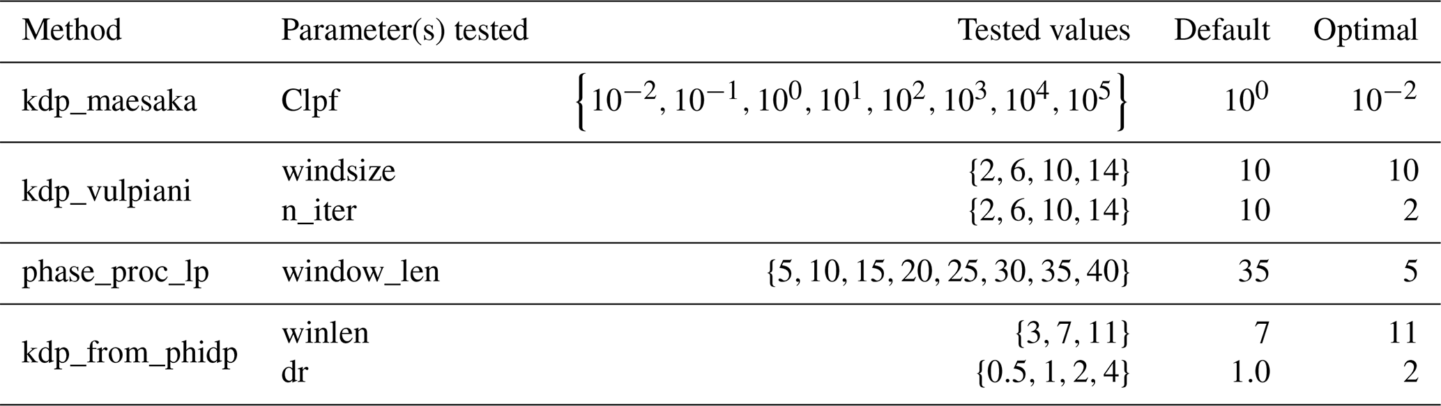
The settings tested for kdp_maesaka, kdp_vulpiani, phase_proc_lp, and kdp_from_phidp are summarized in Table 2, which indicates the tested values, the default value(s) used in the implementation, and the optimal value(s) found in this study.

Table 2 Summary of the parameter settings for each of the optimized methods.

3.1.1 Py-ART's Maesaka method

Py-ART's implementation of the Maesaka et al. (2012) method, kdp_maesaka, features the optimizing parameter Clpf, which regulates the low-pass filter in Φ_DP. The low-pass filter controls the degree of smoothing of Φ_DP, with higher Clpf values producing smoother Φ_DP profiles. In kdp_maesaka, the default value of Clpf is 1.0, and this value is scaled by the range resolution of the radar to match the resolution of the constraints applied to Φ_DP. The scaling is proportional to the fourth power of the range resolution of the radar, and if we were to compare to the values used in Maesaka et al. (2012), a value of 1.0 corresponds to 10¹⁰ for the Vantaa radar's range resolution of 500 m. In Maesaka et al. (2012), Clpf values from 10⁹ to 10¹³ were tested on one rainfall case using a 250 m range resolution X-band radar. Their results show that values closer to 10¹³ suppressed fine-scale precipitation features while producing a smooth and clean K_DP, whereas values closer to 10⁹ preserved fine-scale features while including substantially more noise. These results lead us to test values from 10⁸ to 10¹⁵, corresponding to 10⁻² and 10⁵ in kdp_maesaka and accounting for the Vantaa radar's range resolution. Figure 4a–h show scatterplots of K_DP estimates using kdp_maesaka as a function of Z_H for different Clpf values. All scatterplots show overall accurate and precise K_DP estimates within the Z_H range of 0–30 dBZ. This result implies that the subset of Clpf values studied produces sufficiently smoothed Φ_DP to reduce the impact of noise in light precipitation. However, the effects of excessive smoothing are observed in the range of 40–50 dBZ, where K_DP noticeably underestimates $K_{\mathrm{DP}}^{\mathrm{sc}}$. By comparing the scatterplots from Clpf = 10⁻² to Clpf = 10⁵ in the Z_H interval of 40–50 dBZ, the underestimation of K_DP is stronger with increasing Clpf.

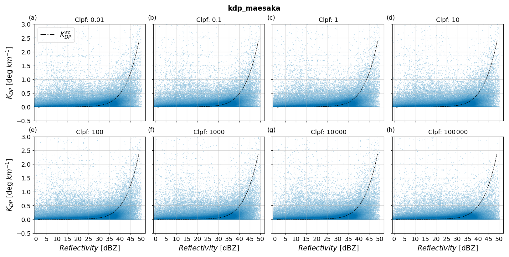
Figure 4 Scatterplots of estimated K_DP from kdp_maesaka as a function of reflectivity and for various values of Clpf. Panels (a)–(h) show results with Clpf values from 10⁻² to 10⁵. The dashed black line corresponds to $K_{\mathrm{DP}}^{\mathrm{sc}}$.

To capture the influence of Clpf on the errors when estimating K_DP as a function of precipitation intensity, Fig. 5a and b show NRMSE and the normalized bias of K_DP estimates with varying Clpf. The smaller and more consistent NRMSEs in regions of Z_H ≥ 35 dBZ in Fig. 5a indicate that kdp_maesaka reaches stable solutions for all Clpf values tested. However, Clpf of 10⁵ showed the largest variability when transitioning from lowest to highest Z_H among the values tested, producing the largest NRMSE for Z_H ≥ 35 dBZ and the lowest otherwise. The underestimation of K_DP using 10⁵ is evidenced in Fig. 5b for Z_H ≥ 35 dBZ, where the results were the most negatively biased. The biases from the remaining parameters were equally consistent and smaller.

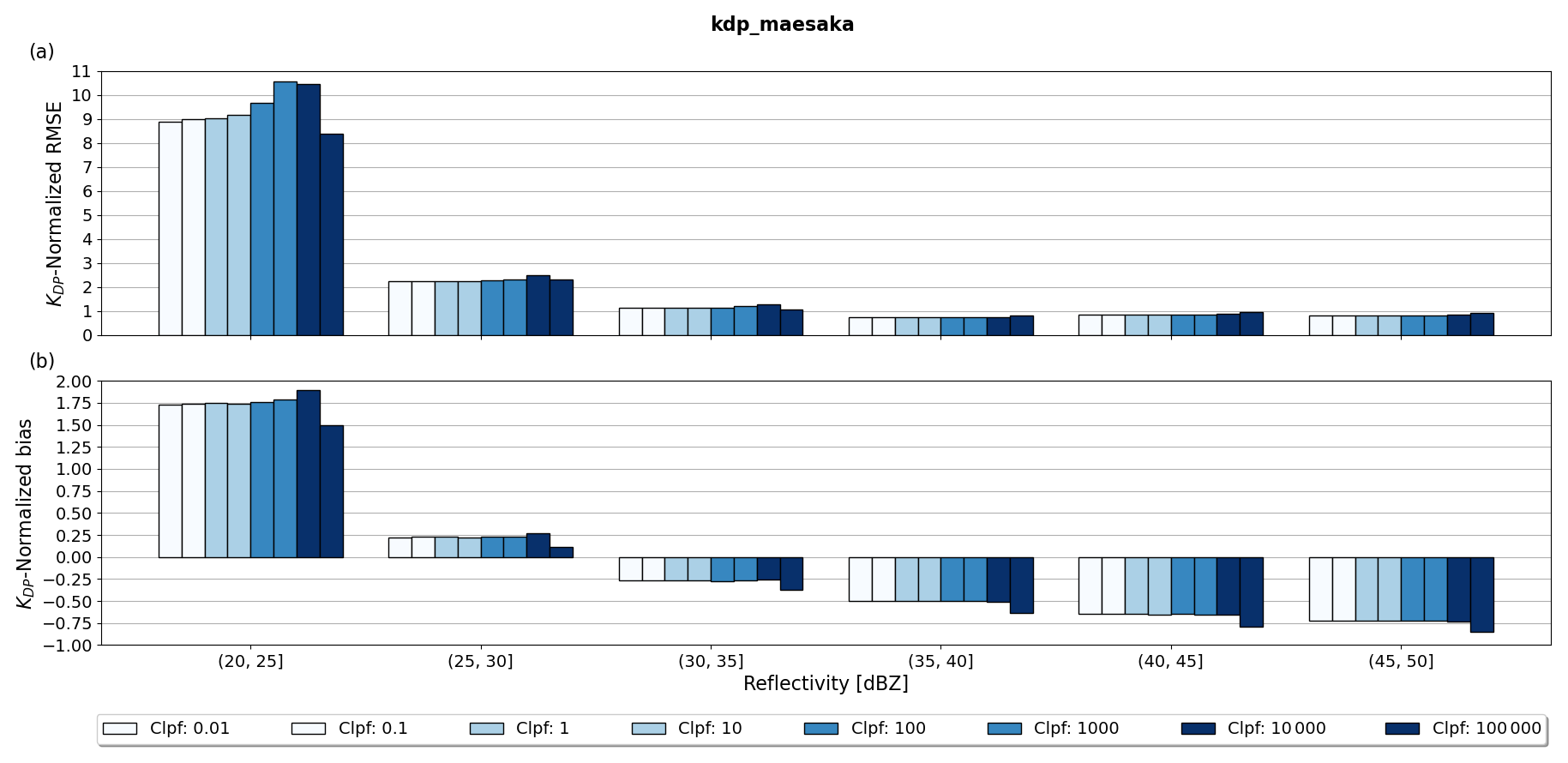
Figure 5 Panel (a) shows RMSE normalized by the interval-averaged $K_{\mathrm{DP}}^{\mathrm{sc}}$ of kdp_maesaka relative to $K_{\mathrm{DP}}^{\mathrm{sc}}$ as a function of reflectivity and for various values of Clpf; panel (b) shows the same as panel (a) but for the normalized bias metric.

Our results show that larger values of Clpf lead to larger errors due to oversmoothing of Φ_DP. Overall, kdp_maesaka performs consistently when precipitation intensities reach 35 dBZ. The Clpf yielding the smallest 35–50 dBZ averaged NRMSE was 10⁻².

3.1.2 Py-ART's Vulpiani method

Py-ART's implementation of the Vulpiani et al. (2012) method, kdp_vulpiani, features two optimizing parameters: windsize (the number of gates used for estimating K_DP) and n_iter (the number of re-estimations of K_DP per window). Higher values of these parameters result in smoother Φ_DP profiles. Reimel and Kumjian (2021) found various parameter combinations that worked well depending on precipitation complexity, leading us to test combinations from 2 to 14 for both parameters. Figure 6a–p show scatterplots comparing the performance of kdp_vulpiani for different values of windsize and n_iter when estimating K_DP. Figure 6a shows the scatter of K_DP using the largest settings tested, whereas Fig. 6p shows the results for the smallest. Each row holds windsize constant, while each column holds n_iter constant. In the scatterplot from Fig. 6a with windsize = 14 and n_iter = 14, the data are predominantly clustered under $K_{\mathrm{DP}}^{\mathrm{sc}}$ for Z_H ≥ 35 dBZ, indicating underestimation of K_DP. For Z_H < 35 dBZ, this parameter setting produces accurate and precise results. The scatterplots for smaller setting values, i.e., towards Fig. 6p, are slightly more accurate, albeit significantly less precise; the scatterplot from Fig. 6p with windsize = 2 and n_iter = 2 shows a wider spread of K_DP data for all Z_H values, although with slightly enhanced clustering of data around $K_{\mathrm{DP}}^{\mathrm{sc}}$ for Z_H ≥ 35 dBZ. These results indicate a trade-off between precision and accuracy when varying windsize and n_iter from 14 to 2. In particular, larger settings favored precision while degrading accuracy, and smaller settings favored accuracy with degraded precision.

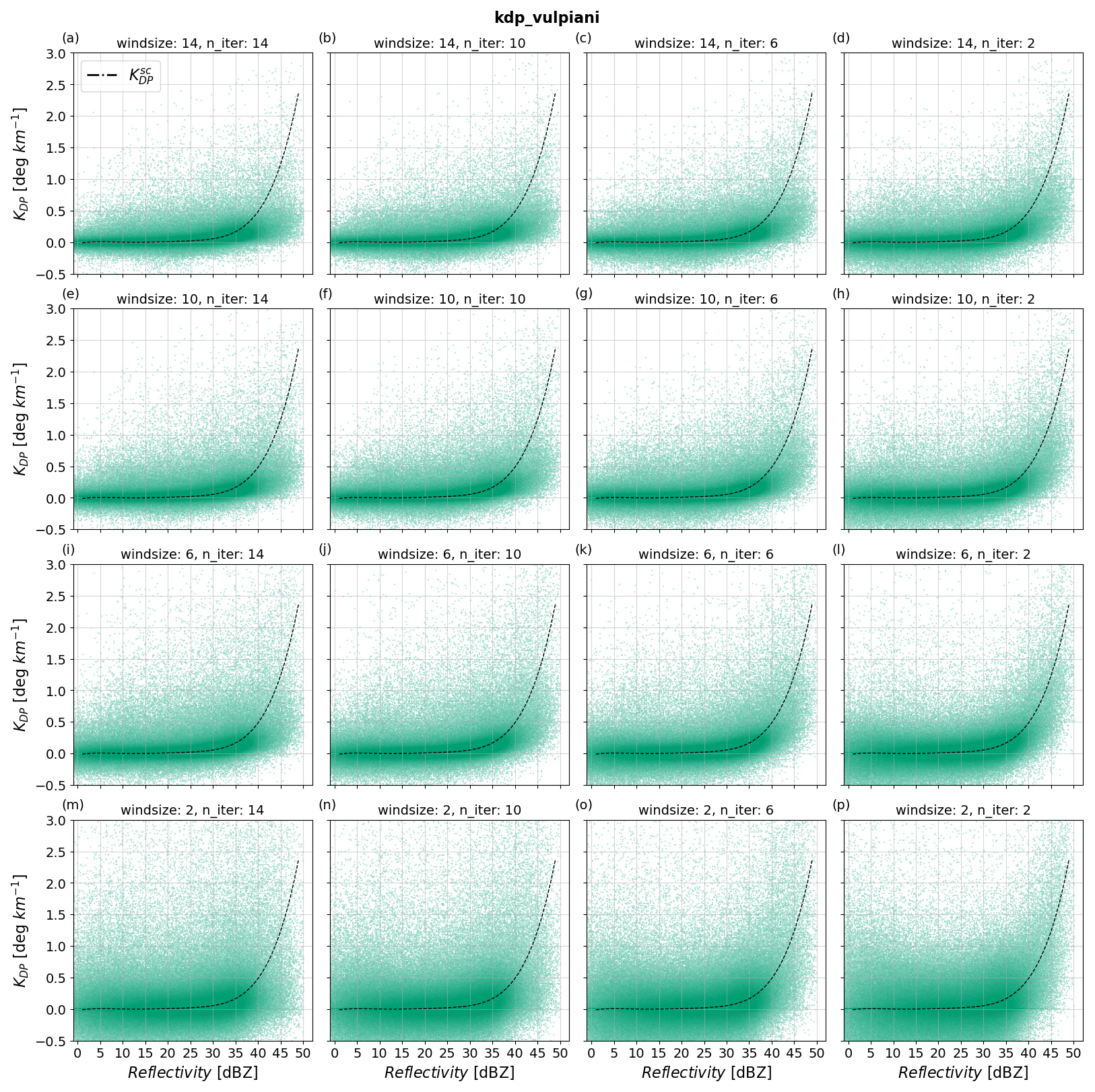
Figure 6 Scatterplots of estimated K_DP from kdp_vulpiani as a function of reflectivity and for various values of windsize and n_iter. Panels (a)–(p) show results with (windsize, n_iter) tuple values from (14, 14) to (2, 2), decreasing windsize with increasing rows. The dashed black line corresponds to $K_{\mathrm{DP}}^{\mathrm{sc}}$.

To further analyze the trade-off between accuracy and precision when varying windsize and n_iter in kdp_vulpiani, Fig. 7a–b show the NRMSE and normalized bias of K_DP estimates with varying windsize and n_iter as a function of Z_H. Figure 7a shows that a windsize of 2 yielded the worst performance, implying that the gain in accuracy by including fine-scale fluctuations in Φ_DP is not enough to compensate for the increased errors due to the inclusion of outliers. On the other hand, a windsize of 14 shows good performance across the entire Z_H range. However, the predominantly negative normalized bias of a windsize of 14 relative to the smaller counterparts in Fig. 7b indicates that the larger windsize leads to more underestimation of K_DP than lower windsize values. The consistent errors when varying n_iter in Fig. 7a indicate that this parameter setting does not impact the performance of kdp_vulpiani as strongly as windsize does, especially in low Z_H. However, results from Fig. 7b suggest that smaller n_iter significantly reduces the underestimation of K_DP estimates when the windsize is large. Our results strongly resemble those reported in Reimel and Kumjian (2021), indicating that a smaller number of iterations and moderate window sizes significantly enhance the performance of kdp_vulpiani. In particular, among the RMSE heat maps of kdp_vulpiani shown in Reimel and Kumjian (2021), windsize = 10 and n_iter = 2 produced the best results, coinciding with the smallest 35–50 dBZ averaged NRMSE in this study.

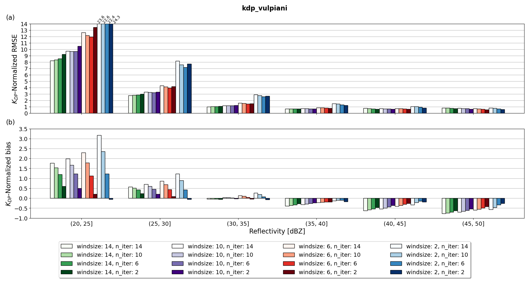
Figure 7 Panel (a) shows RMSE normalized by the interval-averaged $K_{\mathrm{DP}}^{\mathrm{sc}}$ of kdp_vulpiani relative to $K_{\mathrm{DP}}^{\mathrm{sc}}$ as a function of reflectivity and for various values of windsize and n_iter; panel (b) shows the same as panel (a) but for the normalized bias metric.

3.1.3 Py-ART's linear programming method

Py-ART's implementation of an LP method proposed in Giangrande et al. (2013), phase_proc_lp, allows the user to tune the window length to smooth Φ_DP, window_len, and two intertwined parameters constraining the K_DP output via self-consistency relations: self_const and coef. The former is the weight of the self-consistency constraint and the latter is the exponent in the self-consistency relation linking K_DP to Z_H, which is given in Giangrande et al. (2013) as $a{Z}_{\mathrm{H}}^b$ but is expressed in phase_proc_lp as $({\mathrm{10}}^{\mathrm{0.1}\times Z_{\mathrm{H}}}{)}^{\mathrm{coef}}/$self_const. Since information about the expected K_DP was known beforehand, given by $K_{\mathrm{DP}}^{\mathrm{sc}}$, we provided the method with the optimal values of self_const = 10⁴ and coef = 0.914. In this way, the parameter optimization of phase_proc_lp was focused solely on window_len variations.

The parameter window_len defines the window length for smoothing of the LP-processed Φ_DP field before K_DP is estimated. The default setting of this parameter is 35, indicating a smoothing window length of 17.5 km for a range resolution of 500 m. To include finer-scale precipitation features (e.g., ∼ 2.5 km), phase_proc_lp was tested with window_len values ranging from 5 to 40. Figure 8a–h show scatterplots comparing the performance of phase_proc_lp for different settings of window_len estimating K_DP. Each panel from Fig. 8a to h shows K_DP estimated using window lengths from 5 to 40 in intervals of 5. The scatterplot from Fig. 8a with window_len = 5 shows data points predominantly clustered around $K_{\mathrm{DP}}^{\mathrm{sc}}$ across the entire Z_H range, indicating strong correlation between K_DP and $K_{\mathrm{DP}}^{\mathrm{sc}}$. Even in high Z_H ranges (i.e., ≥ 35 dBZ), the tight correlation between K_DP and $K_{\mathrm{DP}}^{\mathrm{sc}}$ holds, indicating high accuracy and precision of K_DP in the presence of heavy precipitation. The accuracy and precision of K_DP relative to $K_{\mathrm{DP}}^{\mathrm{sc}}$ decreases progressively when window_len increases, indicated by the spreading and downward shifting of the K_DP estimates relative to $K_{\mathrm{DP}}^{\mathrm{sc}}$. Especially for the range Z_H ≥ 35 dBZ, the scatterplots from Fig. 8e to h, with window_len from 25 to 40, respectively, show substantial underestimation of K_DP relative to $K_{\mathrm{DP}}^{\mathrm{sc}}$, indicating stronger oversmoothing of Φ_DP for larger values of window_len. Comparing the scatterplots, window_len = 5 undoubtedly shows the best performance of phase_proc_lp. This result agrees with phase_proc_lp window_len experiments by Li et al. (2023) in an extremely heavy precipitation event, where small window_len yielded the best performance. Compared to the phase_proc_lp experiments by Reimel and Kumjian (2021), our results suggest that smaller window_len produce overall more accurate K_DP estimates. However, the influence of the self-consistency constraints proposed in Giangrande et al. (2013) plays a key role in this aspect; if optimal self-consistency constraints are not provided or do not match theoretical expectations, the precision and accuracy in K_DP significantly decreases, and larger window_len values compensate for this by oversmoothing Φ_DP (see Appendix A for results of the performance of phase_proc_lp with very little influence of self-consistency constraints).

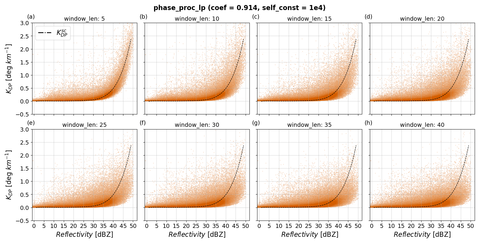
Figure 8 Scatterplots of estimated K_DP from phase_proc_lp as a function of reflectivity and for various values of window_len. Panels (a)–(h) show results with window_len values from 5 to 40 when fixing coef at 0.914 and self_const at 10⁴. The dashed black line corresponds to $K_{\mathrm{DP}}^{\mathrm{sc}}$.

To further investigate the effects of window_len on the performance of phase_proc_lp, Fig. 9a–b show the NRMSE and normalized bias of K_DP estimates with varying window_len as a function of Z_H. In agreement with the patterns observed in the scatterplots in Fig. 8, window_len = 5 produced the best performance compared to other parameter settings. Interestingly, even in light precipitation (e.g., Z_H < 30 dBZ), smaller values of window_len produced the best NRMSE metrics, indicating that larger window_len do not further improve the precision of phase_proc_lp. Instead, larger window_len enhanced the bias of K_DP relative to $K_{\mathrm{DP}}^{\mathrm{sc}}$, as shown in Fig. 9b. The parameter window_len = 5 produced undoubtedly the best metrics for phase_proc_lp, and it was selected as the optimal parameter.

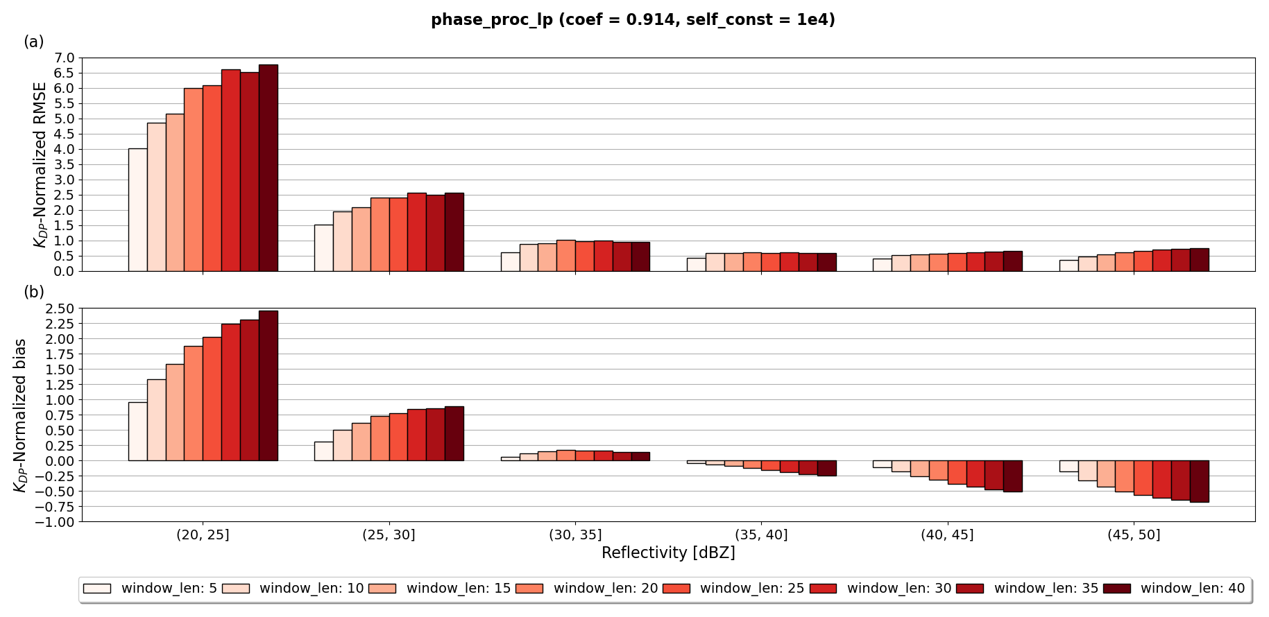
Figure 9 Panel (a) shows RMSE normalized by the interval-averaged $K_{\mathrm{DP}}^{\mathrm{sc}}$ of phase_proc_lp relative to $K_{\mathrm{DP}}^{\mathrm{sc}}$ as a function of reflectivity and for various values of window_len; panel (b) shows the same as panel (a) but for the normalized bias metric.

3.1.4 ωradlib's Vulpiani method

ωradlib's implementation of the Vulpiani et al. (2012) method, kdp_from_phidp, features two optimizing parameters: winlen (the number of gates used to reconstruct Φ_DP) and dr (the gate length resolution in km). We tested winlen values from 3 to 11 and dr values from 0.5 to 4. Figure 10a–l show scatterplots of K_DP estimates using kdp_from_phidp when varying the settings of winlen and dr. Each row of scatterplots holds winlen constant, while decreasing dr from left to right. Similarly, each column of scatterplots holds dr constant, while decreasing winlen from top to bottom. The scatterplot in Fig. 10a, with winlen = 11 and dr = 4, shows K_DP clustered predominantly around 0 ° km⁻¹ across the entire Z_H range, indicating substantial oversmoothing of Φ_DP. Even for Z_H ≥ 30 dBZ, the noticeable underestimation of K_DP relative to $K_{\mathrm{DP}}^{\mathrm{sc}}$ indicates that kdp_from_phidp is not able to capture signatures of heavy precipitation for large winlen and dr settings. Moving towards the scatterplot in Fig. 10d, a smaller dr enhances the accuracy of kdp_from_phidp, particularly for Z_H ≥ 30 dBZ. However, the gain in accuracy comes together with a loss in precision in K_DP estimates, indicated by the wider spread of the data. In addition, decreasing dr makes kdp_from_phidp more prone to the inclusion of outliers, illustrated by data points with K_DP > 1 ° km⁻¹, even for Z_H ≤ 20 dBZ. The scatterplots in Fig. 10e–h follow the same behavior as in the first row except for a wider spread of data, suggesting that decreasing winlen while holding dr constant overall reduces the precision of kdp_from_phidp. When moving from Fig. 10e to h, the accuracy of K_DP estimates increases while precision decreases with decreasing dr. In the last row, i.e., from Fig. 10i to l, K_DP estimates are the most scattered for the same dr, indicating a loss in precision of kdp_from_phidp when reducing winlen. The scatterplot in Fig. 10l with the smallest parameter settings tested (winlen = 3 and dr = 0.5) resembles a scatterplot of random noise with no significant clustering of data, suggesting extremely poor correlation relative to $K_{\mathrm{DP}}^{\mathrm{sc}}$. Comparing the scatterplots row-wise and column-wise, decreasing winlen or dr significantly degrades the precision of the method. However, the effect on the accuracy is more complex; simultaneously setting winlen and dr to large values leads to substantial underestimation of K_DP, whereas small values lead to noisy K_DP. These results suggest that the effects of varying winlen and dr on the performance of kdp_from_phidp are strongly intertwined, requiring more analysis of the trade-off between accuracy and precision offered by variations in these parameters.

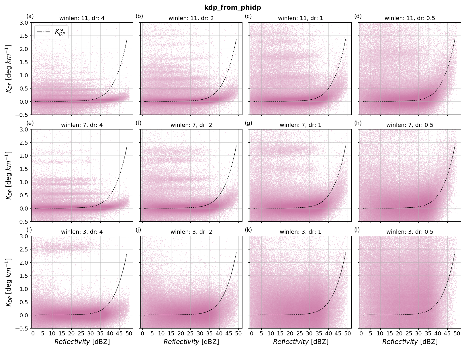
Figure 10 Scatterplots of estimated K_DP from kdp_from_phidp as a function of reflectivity and for various values of winlen and dr. Panels (a)–(l) show results with (winlen, dr) tuple values from (11, 4) to (3, 0.5); winlen decreases in intervals of 4 per row, whereas dr decreases by half per column. The dashed black line corresponds to $K_{\mathrm{DP}}^{\mathrm{sc}}$.

To analyze the trade-off between accuracy and precision when using winlen and dr in kdp_from_phidp, Fig. 11a–b show the NRMSE and normalized bias of K_DP estimates with varying winlen and dr as a function of Z_H. Even though Fig. 11a has been clipped at 5.0, it is important to note the significantly high values when using the smallest dr (97.6, 135.4, and 278.6 for winlen of 11, 7, and 3, respectively). The predominantly higher NRMSE values with the smallest dr indicate that the precision of kdp_from_phidp reduces significantly with dr < 1 for any winlen tested. An exception occurs in the Z_H interval (45,50] dBZ, where the smallest dr yield the best metrics due to slight improvements in the accuracy. Despite the limited amount of data within this Z_H interval (see Fig. 3), the clustering of K_DP around $K_{\mathrm{DP}}^{\mathrm{sc}}$ in Fig. 10 and the small normalized biases in Fig. 11b suggest that accuracy improved slightly for the smallest dr. The smaller NRMSE with high dr in Fig. 11a is counterbalanced by the predominantly larger negative bias for larger dr in Fig. 11b. This implies that larger dr values in kdp_from_phidp lead to the underestimation of K_DP for all winlen tested. As a conclusion, combining large winlen with smaller dr produces the best performance for heavier precipitation (i.e., Z_H > 30 dBZ), whereas combining large winlen with larger dr produces the best results for light precipitation. Overall, small values of winlen reduce the precision significantly in the method without improving accuracy. The parameter setting with the smallest 35–50 dBZ averaged NRMSE was winlen = 11 and dr = 2.

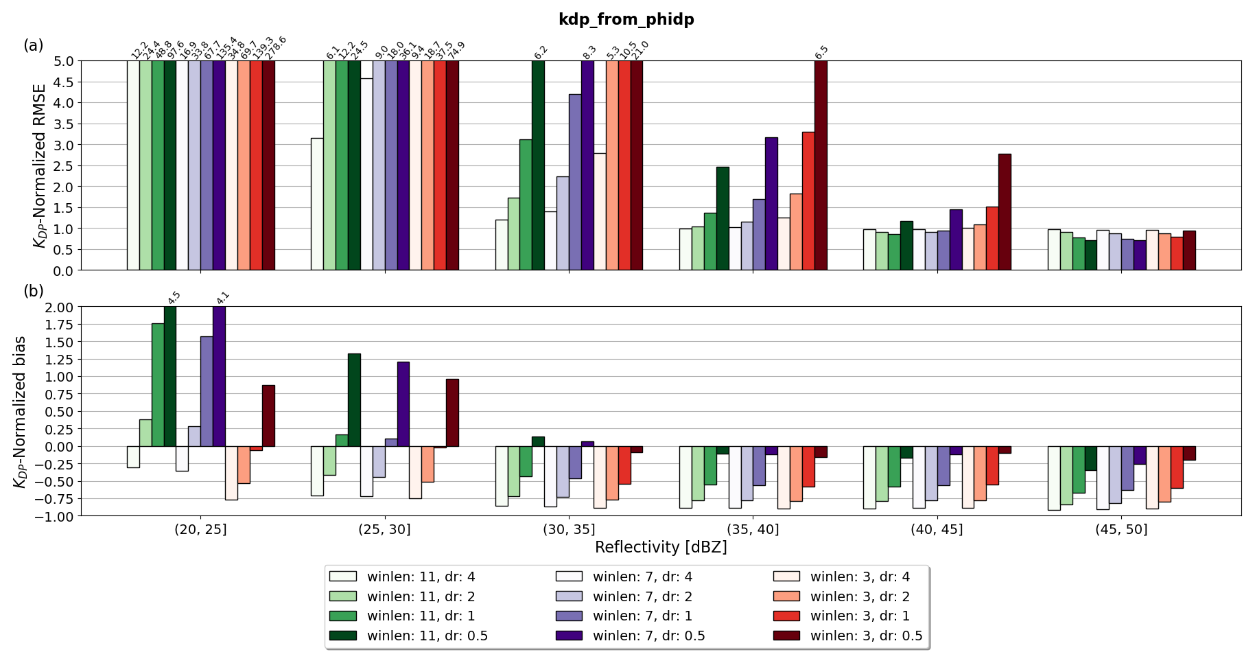
Figure 11 Panel (a) shows RMSE normalized by the interval-averaged $K_{\mathrm{DP}}^{\mathrm{sc}}$ of kdp_from_phidp relative to $K_{\mathrm{DP}}^{\mathrm{sc}}$ as a function of reflectivity and for various values of winlen and dr; panel (b) shows the same as panel (a) but for the normalized bias metric. The numbers on top of the bars indicate the values of the metric exceeding the y-axis limit selected.

3.2 Performance assessment of methods relative to $K_{\mathrm{DP}}^{\mathrm{sc}}$

The performance of the methods is analyzed qualitatively in Sect. 3.2.1 and quantitatively in Sect. 3.2.2. For these analyses, we used the parameter-optimized kdp_maesaka, kdp_vulpiani, phase_proc_lp, and kdp_from_phidp and included kdp_schneebeli and kdp_iris.

3.2.1 Qualitative assessment

We qualitatively assessed the precision and accuracy of the estimated K_DP using scatterplots of K_DP vs. Z_H for each method. Figure 12 shows six scatterplots comparing the performance of kdp_maesaka, kdp_vulpiani, phase_proc_lp, kdp_from_phidp, kdp_schneebeli, and kdp_iris at estimating K_DP. Each scatterplot illustrates the relationship between estimated K_DP (y axis) relative to Z_H (x axis) against benchmarking $K_{\mathrm{DP}}^{\mathrm{sc}}$ (dashed black line). For the parameter-optimized methods in Fig. 12a–d, the optimal parameter selected is indicated in the panel title together with the method's name. Comparing the scatterplots, phase_proc_lp demonstrates the highest accuracy and precision, evidenced by the data narrowly clustered around $K_{\mathrm{DP}}^{\mathrm{sc}}$ across the entire Z_H range. The kdp_from_phidp and kdp_schneebeli methods show the least accuracy and precision, with a broader spread and more outliers, particularly when Z_H < 30 dBZ. For higher Z_H values, even though kdp_from_phidp shows better precision but worse accuracy than kdp_schneebeli, these two methods strongly underestimate K_DP, evidenced by the predominant clustering of K_DP estimates below 0.5 ° km⁻¹. The kdp_maesaka method shows less scattering of K_DP estimates compared to kdp_from_phidp and kdp_schneebeli, indicating higher precision and accuracy, particularly for Z_H < 30 dBZ. However, for Z_H ≥ 30 dBZ, the performance of kdp_maesaka deteriorates rapidly, as shown by the broader spread and significant underestimation of K_DP relative to $K_{\mathrm{DP}}^{\mathrm{sc}}$. The kdp_vulpiani and kdp_iris methods show moderate performance, with better accuracy and precision than kdp_from_phidp, kdp_schneebeli, and kdp_maesaka but worse performance than phase_proc_lp. Between the kdp_vulpiani and kdp_iris methods, kdp_vulpiani shows better correlation of K_DP estimates with $K_{\mathrm{DP}}^{\mathrm{sc}}$ for Z_H ≥ 35 dBZ, indicating higher accuracy in heavier precipitation. However, kdp_iris shows less scattering across the entire Z_H range, indicating overall higher precision than kdp_vulpiani. The kdp_vulpiani, kdp_from_phidp, kdp_schneebeli, and kdp_iris methods include negative K_DP values, which should not be expected in rain observations. These negative estimates predominantly show up in lighter precipitation (i.e., Z_H < 30 dBZ), indicating that they are most likely produced by noise in Φ_DP. However, the inclusion of negative K_DP estimates is useful, for instance, in the detection of snow crystals, allowing kdp_vulpiani, kdp_from_phidp, kdp_schneebeli, and kdp_iris to be used in a wider range of applications compared to kdp_maesaka and phase_proc_lp. The relatively high accuracy and precision of kdp_iris and kdp_vulpiani, together with the inclusion of negative K_DP estimates, leave these two methods as candidates well-suited for QPE and calibration and hydrometeor classification routines.

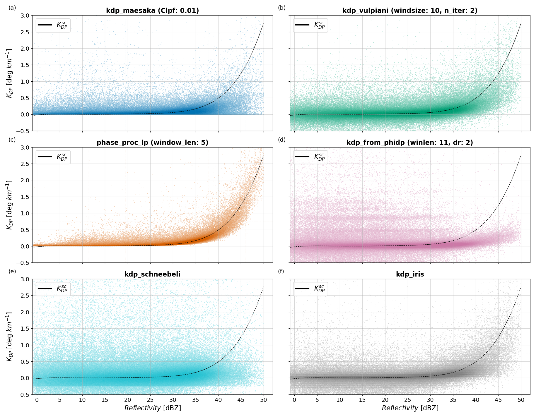
Figure 12 Scatterplot of estimated K_DP from each parameter-optimized method relative to $K_{\mathrm{DP}}^{\mathrm{sc}}$ as a function of reflectivity. Panels (a)–(f) show kdp_maesaka, kdp_vulpiani, phase_proc_lp, kdp_from_phi_dp, kdp_schneebeli, and kdp_iris, respectively. The dashed black line corresponds to $K_{\mathrm{DP}}^{\mathrm{sc}}$.

3.2.2 Quantitative assessment

The quantitative assessment of the methods was achieved through the metrics of NRMSE and normalized bias and complemented with statistics from the Wasserstein distance (WD) (Ramdas et al., 2015). The WD measures the similarity between two cumulative distributions, given in this study by the K_DP estimated by each method and $K_{\mathrm{DP}}^{\mathrm{sc}}$. On the one hand, NRMSE and normalized bias computed as a function of Z_H, allow the assessment of the relative accuracy and precision of the methods based on precipitation intensities. The WD, on the other hand, estimated from each radar scan independently and with statistics over the entire set of scans, allows the assessment of the relative consistency and robustness of the methods.

Figure 13a–b show the NRMSE and normalized bias of estimated K_DP for each method. Overall, phase_proc_lp shows the best performance, as evidenced by the lowest NRMSE values in Fig. 13a and moderately low bias in Fig. 13b across all Z_H intervals. In contrast, kdp_schneebeli shows the worst performance among the methods, indicated by the highest NRMSE values and moderately high bias across all Z_H intervals. The kdp_from_phidp method shows substantially higher NRMSE values than kdp_maesaka, kdp_vulpiani, phase_proc_lp, and kdp_iris but is significantly smaller than kdp_schneebeli, particularly for the smallest Z_H values. The relatively small bias of kdp_from_phidp when NRMSE values are substantially high is explained by the positive-to-negative symmetrical spread of K_DP estimates around the x axis, indicating poor precision. Additionally, the persistently negative and large normalized bias of this method relative to the other methods indicates that kdp_from_phidp underestimates K_DP the most. The kdp_maesaka, kdp_vulpiani, and kdp_iris methods have moderate NRMSE values, performing better than kdp_schneebeli and kdp_from_phidp but not as well as phase_proc_lp. Among these three methods, kdp_maesaka has the smallest NRMSE values for Z_H ≤ 35 dBZ but the largest when Z_H ≥ 40 dBZ. The relatively large positive bias of kdp_maesaka when Z_H < 30 is a direct consequence of the exclusion of negative K_DP estimates. However, the persistently larger negative bias of kdp_maesaka relative to kdp_vulpiani and kdp_iris when Z_H ≥ 30 dBZ indicates stronger underestimation of K_DP and thus less accuracy. These results indicate that in comparison to other methods, kdp_maesaka performs slightly better in light precipitation (i.e., Z_H <30 dBZ) but worse in heavier precipitation. Between kdp_vulpiani and kdp_iris, kdp_iris shows overall smaller NRMSEs and normalized bias, indicating higher accuracy and precision than kdp_vulpiani.

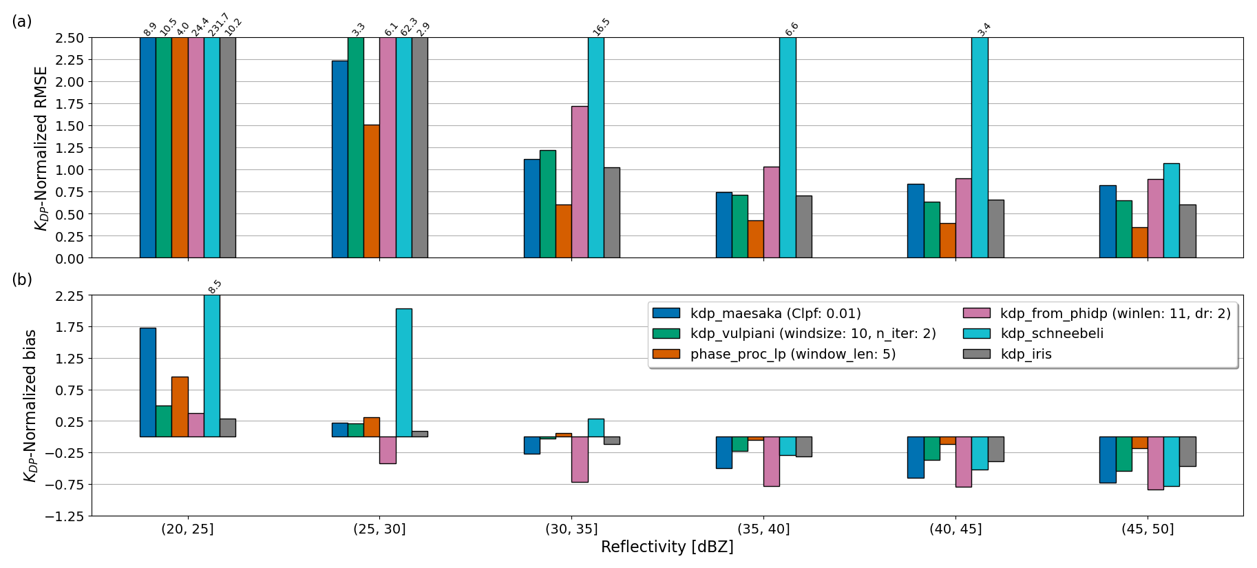
Figure 13 Panel (a) shows the bias of estimated K_DP from each parameter-optimized method relative to $K_{\mathrm{DP}}^{\mathrm{sc}}$ as a function of reflectivity; panel (b) shows the same as panel (a), but the bias is normalized by interval-averaged $K_{\mathrm{DP}}^{\mathrm{sc}}$. The numbers on top of the bars indicate the values of the metric exceeding the y-axis limit selected.

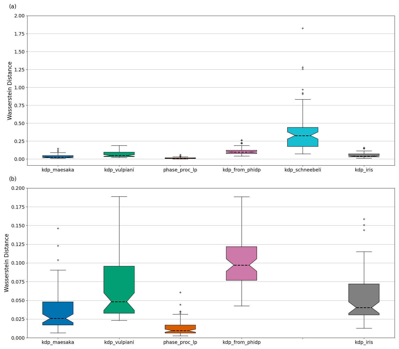
Figure 14 Panel (a) shows the boxplot of the WD computed for each parameter-optimized method; panel (b) shows the same as panel (a) but excluding kdp_schneebeli for better visualization of the better-performing methods. The boxplots display the WD median (dashed black line), IQRs (boundaries of the box), 1.5× IQR (whiskers), and the outliers (black crosses).

Complementary to the NRMSE and normalized bias metrics, we evaluated the consistency and robustness of the methods using the Wasserstein distance (WD). The WD was computed for each radar scan independently using the wasserstein_distance module from SciPy (Virtanen et al., 2020). Then, the statistics from the estimated WD values for all scans were visualized and analyzed using boxplots. Figure 14 consists of two panels comparing the WD boxplots of the methods. Figure 14a compares the WD for all methods, including kdp_schneebeli, which presented a significantly large WD. Figure 14b presents the same data as (a) but excludes kdp_schneebeli to better compare the remaining methods. Each boxplot summarizes the statistics of estimated WDs by showing the median (dashed black line), interquartile ranges (IQR), 1.5× IQR (whiskers), and outliers (crosses). The insights provided by the boxplots in this analysis are twofold. First, a WD median closer to 0 indicates higher similarity between the cumulative distributions of a method's estimated K_DP and that from $K_{\mathrm{DP}}^{\mathrm{sc}}$, ultimately indicating higher accuracy. Second, a narrower IQR indicates less variability in a method's performance between scans, indicating higher consistency.

In Fig. 14a, the x axis lists six methods: kdp_maesaka, kdp_vulpiani, phase_proc_lp, kdp_from_phidp, kdp_schneebeli, and kdp_iris. The y axis measures the WD values ranging from 0 to 2. The boxplot for the kdp_schneebeli method shows the largest WD, with a median of 0.33, an IQR from 0.18 to 0.45, and several outliers. The other methods (kdp_maesaka, kdp_vulpiani, phase_proc_lp, kdp_from_phidp, and kdp_iris) have median WD values ranging from 0.0 to 0.1, with smaller IQRs and fewer outliers. In Fig. 14b, the kdp_schneebeli method is excluded, allowing for a clearer comparison of the kdp_maesaka, kdp_vulpiani, phase_proc_lp, kdp_from_phidp, and kdp_iris methods. The y axis is rescaled to range from 0.0 to 0.2 for better visualization. The phase_proc_lp method has the lowest WD median at 0.01, with a narrow IQR from 0.008 to 0.018. The kdp_from_phidp method has a significantly larger WD median of 0.098 and an IQR from 0.077 to 0.122. The kdp_maesaka and kdp_iris methods have WD medians of 0.026 and 0.041, respectively, with moderate IQRs and few outliers. The kdp_vulpiani method has a moderate WD median of 0.049 but a noticeably wider IQR from 0.033 to 0.096 when compared to kdp_maesaka, phase_proc_lp, kdp_from_phidp, and kdp_iris.

The large WD median of kdp_schneebeli indicates that it performs worse compared to the other methods, overshadowing the performance differences among the remaining methods. Additionally, the large IQR of kdp_schneebeli implies that the method does not perform consistently, thus reducing its reliability. The phase_proc_lp method demonstrates the best and most consistent performance, with the lowest WD median and narrowest IQR. These results additionally indicate that the distribution of K_DP estimated from phase_proc_lp is the closest to $K_{\mathrm{DP}}^{\mathrm{sc}}$. It is important to remember here that phase_proc_lp is supported by self-consistency relations constraining the K_DP estimates based on Z_H observations, ultimately enhancing its accuracy and stability. The moderate IQR and significantly larger WD median of kdp_from_phidp indicate that its performance is consistent, albeit less accurate relative to the other methods. The kdp_vulpiani method, in turn, has a moderate WD median but relatively larger IQR, indicating better accuracy than kdp_from_phidp, although less consistency. The kdp_maesaka and kdp_iris methods show similar consistency and accuracy, evidenced by their relatively low WD medians and moderate IQRs. These findings suggest that while kdp_schneebeli is the least accurate and consistent, the performance among the remaining methods varies, with phase_proc_lp presenting the highest robustness, provided that the method with quality controlled Z_H and optimized self-consistency settings is used.

3.3 Consistency analysis of K_DP retrievals

Each method has a unique combination of mathematical approaches, data requirements, and constraints (see Table 1), indicating uniqueness in the K_DP fields produced. The similarity or dissimilarity of these outputs is not clearly visible from the metrics computed or from the scatterplots displayed in Sect. 3.2. To answer this question, we study the consistency among methods using the K_DP vs. K_DP correlation plots shown in Fig. 15. Each scatterplot in Fig. 15 shows the relationship between K_DP estimated by a method (y axis) with respect to K_DP estimated by a different method (x axis), and the Pearson correlation coefficient (R) is shown in the upper-left corner of each scatterplot. The axes range from −0.5 to 3.0 ° km⁻¹ to include negative K_DP estimates. This part of the analysis does not require any ground-truth framework, allowing the use of the entirety of the radar dataset, i.e., including the attenuated observations (see red data in Fig. 3).

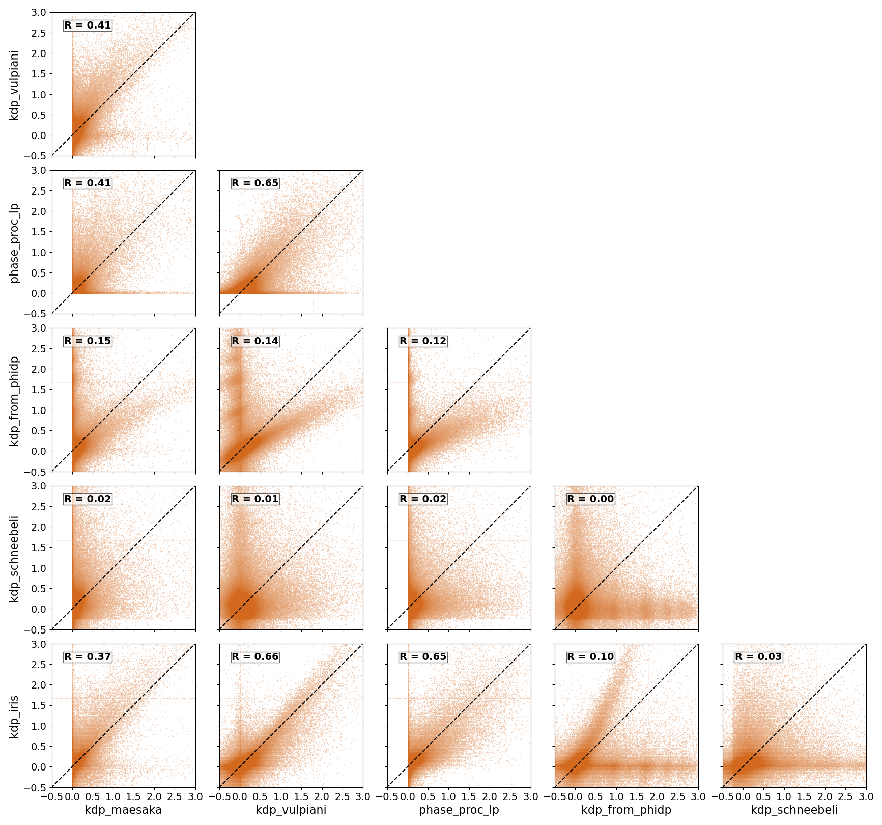
Figure 15 Correlation between the K_DP estimation methods. Each scatterplot shows the relationship between two different methods without repetition, and no method is compared to itself. The x and y axes represent the K_DP estimated by a method, in units of ° km⁻¹. Each panel shows the Pearson correlation coefficient between the two methods compared.

In Fig. 15, the scatterplot of kdp_iris against kdp_vulpiani shows the best correlation among the methods, illustrated by the data significantly clustered along the diagonal and corroborated by the highest R of 0.66. The kdp_iris and kdp_vulpiani methods correlate similarly with phase_proc_lp, indicated by the second-highest R of 0.65 for both. In relation to kdp_maesaka, the consistencies of kdp_iris and kdp_vulpiani are rather moderate, whereas in relation to kdp_from_phidp and kdp_schneebeli, they are significantly poorer. Among the methods, kdp_schneebeli correlates the least with any of the other methods, evidenced by the data widely spread along the axes and showing negligible clustering along the diagonal. In particular, kdp_schneebeli against kdp_from_phidp shows the worst consistency, with R = 0 and the majority of the data clustered around the x and y axes. The phase_proc_lp method correlates moderately with kdp_maesaka, with an R = 0.41, although the scatterplot does not exhibit any particular pattern or clustering of data along the diagonal. Relative to kdp_from_phidp, phase_proc_lp shows significantly lower R despite the clear data correlation off of the diagonal. However, the small R value becomes evident when observing the dense clustering of data around 0 ° km⁻¹ for phase_proc_lp. This result indicates that the consistency between kdp_from_phidp and phase_proc_lp is highly influenced by the negative K_DP estimates in kdp_from_phidp that are mapped to 0 ° km⁻¹ in phase_proc_lp. Overall, the scatterplots show that kdp_from_phidp underestimates K_DP relative to the other methods. The kdp_maesaka method shows no significant correlation with any method, with the largest R being 0.41 relative to both phase_proc_lp and kdp_vulpiani.

4 Conclusions

In this study, we conducted a comprehensive evaluation of several K_DP estimation methods using C-band weather radar data, with a focus on their performance in rainfall observations. We employed a self-consistency framework that links Z_H and Z_dr observations, with K_DP as the basis for our evaluations. This approach allows for the construction of the reference K_DP observations that can be used to assess the accuracy and robustness of the K_DP estimation methods studied. The use of the self-consistency framework requires rather strict quality control, which is described in the paper. In this way, our study focuses on the performance of the methods in highly idealized rainfall observations.

Some (four out of six) of the K_DP estimation methods have user-configurable parameters. Using the evaluation framework proposed, we were able to define optimized parameter settings. Most of the methods showed significant improvement in the performance after the optimization.

By comparing the relative performance of the estimation methods over the range of rain intensities, as characterized by the radar Z_H values, we have found significant differences in the performance of the methods evaluated. Overall, implementations of the Giangrande et al. (2013), Vulpiani et al. (2012), and Wang and Chandrasekar (2009) methods exhibited the lowest NRMSE and normalized biases over the range of Z_H values studied, from 20 to 50 dBZ.

Our comparative analysis revealed that while the implementation of the Giangrande et al. (2013) method stands out for its high accuracy and precision, its performance is heavily dependent on the self-consistency constraint provided. Without proper optimization of the self-consistency relation, linking of Z_H and K_DP, and quality control of Z_H, even the best window length setting for this method can lead to suboptimal results, i.e., higher RMSE and K_DP underestimation at higher Z_H values. It should be noted, however, that the reference framework and the Giangrande et al. (2013) method use self-consistency relations to determine K_DP, and, therefore, the uncertainties are correlated, and part of the reported performance is caused by this dependence. The implementations of Vulpiani et al. (2012) and Wang and Chandrasekar (2009) showed good performance and do not require the use of other radar variables, which potentially make them less sensitive to radar data quality issues, such as calibration and attenuation.

An additional qualitative comparison of the performance of the methods was carried out by computing correlations of derived K_DP values from the dataset that also included attenuated radar observations. The correlation between K_DP values estimated using different methods is not very high. The highest correlation values (0.65–0.66) were observed between the Giangrande et al. (2013), Vulpiani et al. (2012), and Wang and Chandrasekar (2009) methods. This indicates that uncertainty between different precipitation estimates could stem from the differences in the K_DP methods used.

The study is based on a self-consistency framework that limits its use to the cases where no significant attenuation is observed. Additionally, the scope of our study is limited to the Finnish climatology and a single radar frequency, namely C-band radar observations. Despite these limitations, our findings offer valuable guidance for the use of K_DP estimation methods in rainfall observations. These results have significant implications for both operational radar networks and hydrometeorological research, where the accuracy, precision, and stability of K_DP estimates are crucial.

Appendix A: Influence of the self-consistency constraint on phase_proc_lp

Figure A1 shows the same scatterplots as Fig. 8, with K_DP estimated from phase_proc_lp using self_const of 10⁶ instead of 10⁴. The motivation behind this was to study the performance of phase_proc_lp with little influence from self-consistency constraints. In Giangrande et al. (2013), the non-negativity condition in K_DP estimates is ensured by restricting the b vectors: b ≥ 0. In addition, to produce more realistic K_DP estimates, they introduced the self-consistency relation $K_{\mathrm{DP}}\left(Z_{\mathrm{H}}\right)=a{Z}_{\mathrm{H}}^b$ to bound the estimates based on observed Z_H, requiring that the user provide quality controlled data. The restriction of the b vectors becomes $\mathit{b}\ge a{Z}_{\mathrm{H}}^b$, which in phase_proc_lp is implemented as $\mathit{b}\ge ({\mathrm{10}}^{\mathrm{0.1}\times Z_{\mathrm{H}}}{)}^{\mathrm{coef}}/$ self_const. Therefore, a self_const value that is 2 orders of magnitude larger was used in this study to test the performance of phase_proc_lp with a significantly reduced influence of self-consistency constraints. The scatterplots show K_DP data clustered around $K_{\mathrm{DP}}^{\mathrm{sc}}$ up to 35 dBZ. Beyond this threshold, precision and accuracy decay significantly regardless of the window length. However, in scatterplots with larger window lengths, K_DP data are less scattered across the entire Z_H range and are only slightly less accurate after 35 dBZ.

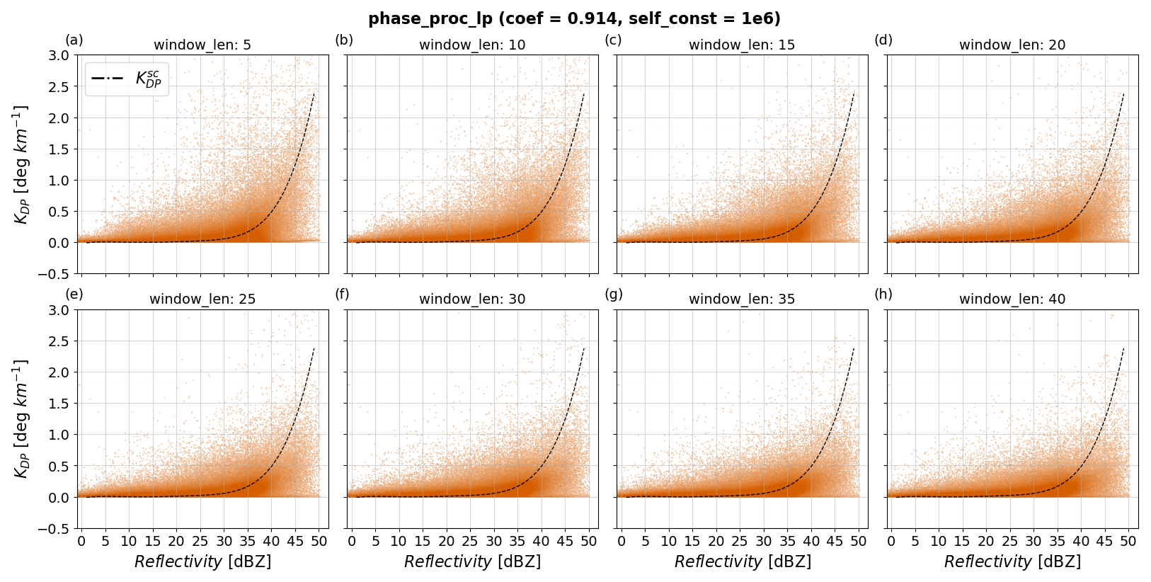
Figure A1 Scatterplots of estimated K_DP from phase_proc_lp as a function of reflectivity and for various values of window_len. Panels (a)–(h) show results with window_len values from 5 to 40 when fixing coef to 0.914 and self_const to 10⁶. The dashed black lines correspond to $K_{\mathrm{DP}}^{\mathrm{sc}}$.

To further investigate the effects of the self-consistency constraint on phase_proc_lp, Fig. A2a–b show the normalized RMSE and bias of K_DP (estimated with self_const = 10⁶) relative to $K_{\mathrm{DP}}^{\mathrm{sc}}$. Interestingly, the normalized RMSE in Fig. A2a behaves inversely to the normalized RMSE in Fig. 9, whereas normalized bias shows similar behavior for both. The opposite behaviors in normalized RMSE results indicate that window length has a strong impact on the performance of phase_proc_lp, depending on whether adequate self-consistency settings were provided; if so, smaller window lengths yield better performance by capturing fine-scale precipitation features, especially in heavy precipitation. In the opposite case, larger window lengths yield better performance by oversmoothing Φ_DP, thus reducing the impact of noise at the expense of losing fine-scale precipitation features. The oversmoothing effect from larger window lengths in K_DP is also implied from the normalized bias shown in Fig. A2b; larger window lengths produced the largest absolute biases at both extremes of the Z_H range. In addition, even though the normalized bias shows similar behavior for self_const = 10⁶ and self_const = 10⁴, the latter produces larger differences between window lengths, indicating that the high accuracy and precision of phase_proc_lp predominates in smaller window lengths, provided that there are adequate self-consistency constraints and quality controlled Z_H.

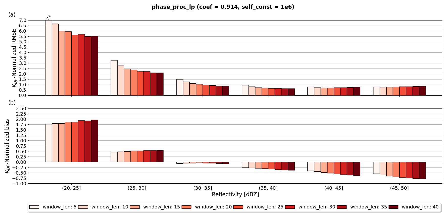
Figure A2 Panel (a) shows RMSE normalized by the interval-averaged $K_{\mathrm{DP}}^{\mathrm{sc}}$ of phase_proc_lp relative to $K_{\mathrm{DP}}^{\mathrm{sc}}$ as a function of reflectivity and for various values of window_len; panel (b) shows the same as panel (a) but for the normalized bias metric.