Bias correction and application of labeled smartphone pressure data for evaluating the best track of landfalling tropical cyclones

Smartphone pressure observations have demonstrated significant potential to complement traditional pressure monitoring. However, challenges remain in correcting biases and further leveraging these observations for practical applications. In this study, we used tropical cyclones (TCs) Lekima in 2019, Hagupit in 2020 and In-fa in 2021 as examples to conduct bias correction on labeled smartphone pressure data from the Moji Weather app. We propose a quality control procedure utilizing random forest machine learning models. By applying this quality control approach to the selected TCs, we discovered that the performance of the method for labeled data significantly surpassed that for unlabeled data developed in a previous study, reducing the mean absolute error from 3.105 to 0.904 hPa. The bias-corrected smartphone data were then supplemented with weather station data for sea-level-pressure analyses and compared with the analyses that used only weather station data. The significantly higher spatial resolution and broader coverage of the smartphone data led to notable differences between the two analysis fields. Additionally, we compared the minimum sea-level pressure of TCs derived from smartphone data, weather station observations and the best-track dataset from the Shanghai Typhoon Institute (STI) of the China Meteorological Administration. We found that the best track published by STI consistently underestimated the minimum sea-level pressure, with a median difference of 0.51 hPa in the three TC cases.

1 Introduction

Meteorological observation data are crucial for the efficacy of early warning systems; however, their discontinuity and inconsistency in time and space often pose challenges. The problem is more severe in many underdeveloped and developing regions due to the lack of funding, technology and infrastructure, as well as backward network construction (Dinku, 2019; Heaney et al., 2016; Thomson et al., 2017). Smartphones with built-in sensors may offer a solution to this problem, as the number of smartphone users has grown to more than 50 % of the population in developing countries, such as China and Mexico (Newzoo, 2023), and as high as 46 % in some underdeveloped parts, such as sub-Saharan Africa (GSMA, 2022). Sensors in smartphones can monitor pressure (Kim et al., 2015; Mass and Madaus, 2014), temperature (Overeem et al., 2013) and radiation (Mei et al., 2015), among which pressure monitoring is more commonly available (Kim et al., 2015). On the one hand, the results of pressure measurements are not easily affected by local observing conditions (Mass and Madaus, 2014). This implies the errors are generally stable and systematic (Price et al., 2018), leading to high-quality surface observations with high spatiotemporal resolution. On the other hand, surface pressure contains important meteorological information and reflects the deep structure of the atmosphere (Mass and Madaus, 2014). Therefore, the smartphone pressure data are valuable and worth studying as a meteorological data source.

While smartphones can provide pressure data with higher spatiotemporal resolution than traditional weather observation networks, they have unique data quality issues. Although pressure records from smartphones and weather stations are highly correlated statistically, noticeable offsets exist between individual smartphones (Price et al., 2018; Hintz et al., 2019). Smartphones can produce pressure measurements that differ from those of the surface stations when users are at high levels in buildings (Li et al., 2021). Traditional quality control methods include the elimination of outliers and screening for statistical, spatial and altitude consistency, which usually leads to a sharp reduction in data volume to about 10 % to 40 % of the original dataset (Madaus and Mass, 2017; Hintz et al., 2019). Recently, machine learning models have been applied to the correction and validation of pressure data. These models rely on the geographical similarity of error distribution (Li et al., 2021; McNicholas and Mass, 2021) for data without user identification and on the relatively stable performance of individual smartphones (McNicholas and Mass, 2018) for data with user identification. (In the rest of this paper we refer to them as “unlabeled data” and “labeled data”, respectively; further explanation can be found in Sect. 2.1.) These methods have their limitations because, even when the models are applied to the same descriptive variables, differences in results may occur among different regions. This variation is attributed to the dependence on sensor performance across different regions and the accuracy of location information.

Another important question is what additional information smartphones provide. Due to their high spatiotemporal resolution, quality-controlled or corrected smartphone pressure data are often used to characterize convective systems at small or mesoscales. Hintz et al. (2019), Li et al. (2021), and McNicholas and Mass (2018) found pressure changes of 1 hPa h⁻¹ at sea level, 0–0.5 hPa min⁻¹ and 1.5 hPa per 15 min at the surface, respectively, within the convective systems they studied. During tropical cyclone (TC) Michael in 2018 in the United States, smartphone pressure data measured the low-pressure value at the TC center more accurately than the conventional Meteorological Assimilation Data Ingest System (McNicholas and Mass, 2021). However, the value was still more than 10 hPa higher than the actual minimum pressure, partly due to the low density of smartphone pressure data along the track of TC Michael; the closest smartphone observation was 5 km away from the TC center. Given the dense population in China, it is interesting to determine if the smartphone pressure observations could provide a better estimate of TC minimum pressure, an important parameter of TC intensity.

The unlabeled smartphone pressure data from China have recently been studied for quality control and application to mesoscale analysis (Li et al., 2021). The labeled data, which can provide higher-quality observations and enable personalized and more accurate analyses, have not been examined in China, especially in densely populated areas. In this study, we present a machine-learning-based method for the bias correction (BC) of labeled smartphone pressure data collected by the Moji Weather app. We evaluate the performance of the approach by comparing the results with those from unlabeled data.

As one of the major weather service applications in China, the Moji Weather app has more than 700 million users and more than 600 million daily weather queries (Moji, 2023a, b). The quality of the unlabeled pressure data provided by Moji Weather has been verified by Cao et al. (2022) and Li et al. (2021). We anticipate that the evaluation of the labeled data from Moji Weather in this study will provide a broader understanding of the smartphone pressure data. In addition, by using the three TC events – Lekima in 2019, Hagupit in 2020 and In-fa in 2021 – as examples, we investigate how the higher spatiotemporal resolution of the smartphone pressure data benefits TC intensity analysis.

This paper is organized as follows. In Sect. 2, we present the data and methods used in this study. Taking TC Lekima in 2019 as an example, Sect. 3 compares the results of corrected labeled and unlabeled pressure data and tests their impact on mesoscale pressure analysis fields. In Sect. 4, we compare the corrected smartphone pressure data with the best-track data released by the Shanghai Typhoon Institute (STI) of the China Meteorological Administration (CMA) for three TCs from 2019 to 2021. Conclusions and discussion are provided in Sect. 5.

2 Data and methods

2.1 Data and quality control

The data used in this study include sea-level-pressure observations from weather stations, smartphone pressure measurements, TC best-track data and supplementary data for machine learning models. More details on these data are provided below:

1. Sea-level-pressure data at 1 h intervals from weather stations are obtained from CMA. There are 11 585, 13 200 and 16 208 atmospheric pressure observation stations in China for the years of 2019 (Fig. 1), 2020 and 2021, respectively.

2. Smartphone pressure data at 1 min intervals are provided by the Moji Weather company. The data include time, latitude and longitude acquired by the weather app when running in the foreground or background, as well as pressure measured by built-in sensors. The data are provided by users who have signed a data-sharing agreement, and each pressure record carries an encrypted user ID that helps to distinguish the source of the data. However, we clearly understand that user IDs are sometimes not available, so we also made a dataset with user IDs removed for comparative experiments. In the rest of this paper, we refer to data without user ID as “unlabeled data” and correspondingly data with user ID as “labeled data”. We strictly adhere to the principle of privacy protection, which ensures all research is conducted at the population level, involving only the analysis of data volume and pressure values. In other words, no information regarding any individual's specific movements is exposed. All research data in this study have been legally verified to comply with all provisions of the Personal Information Protection Law of the People's Republic of China issued on 20 August 2021 (https://www.gov.cn/xinwen/2021-08/20/content_5632486.htm, last access: 7 February 2025), which was confirmed by the legal department of the Moji Weather company.

   In 2019, a total of 83 386 957 users contributed to the pressure observations within the area of 15–55° N and 70–140° E. Eastern China – a TC-prone area – had a higher user density than western China, and the discrepancy is larger in the urban areas (Fig. 2a). The density variation implies that the detected TC tracks usually pass through areas with dense observations. The number of individual user observations was relatively small, averaging fewer than 125 over an entire year (10.4 per month) in most urban areas (Fig. 2b), compared to 774 over 16.5 months (46.9 per month) in McNicholas and Mass (2021). This may limit the complexity and performance of the correction models for each individual user. The relatively small number of observations from individual users may be attributed to differences in the information collection system and user usage habits. However, a relatively large number of users can somewhat compensate for this shortcoming. Users with more than 100 and 1000 observations accounted for approximately 17.6 % and 2.5 % of the 83 386 957 samples, contributing 88.9 % and 42.6 % to the total data volume, respectively (Fig. 2c and d). To strike a balance between providing more data for each user's correction model and maximizing the total amount of data retained, we selected users with more than 100 observations for the correction. The total number of these users is 14 676 104.

   The quality control of smartphone pressure data is performed in three steps. (1) Following the practice of Kim et al. (2015) and Madaus and Mass (2017), pressure values outside the normal range (890–1080 hPa) are considered outliers and eliminated. (2) Reference sea-level pressure at the location of the smartphone is estimated by spatial interpolation of weather station data, and smartphone pressures deviating by more than 15 hPa from the reference are discarded to eliminate data from low-quality sensors or at a high altitude. (3) Latitude, longitude and pressure are retained to four decimal places, and only one record of duplicate data for the same hour is retained. By doing so, the adverse effect of excessive data duplication on the machine learning correction model could be largely avoided.

   Due to the different temporal resolutions of smartphone and weather station datasets, we aligned the weather station pressure with the smartphone pressure at 20 min intervals centered on the hour and discarded any other smartphone data during the quality control procedure. For unlabeled data, considering that there are indistinguishable observations of the same latitude, longitude and time, especially in urban high-rise areas, we created “smartphone sites” by calculating the number, mean pressure and standard deviation of the overlapping smartphone observations. Furthermore, we performed BC on the smartphone pressure data using a machine learning scheme. This is crucial for more accurately estimating the extremely low pressures, such as those found at the center of TCs. The methods and the results will be discussed in detail in Sect. 3.

3. The tropical cyclone best-track data used are provided by STI (Lu et al., 2021; Ying et al., 2014) (https://tcdata.typhoon.org.cn/en/zjljsjj.html, last access: 7 February 2025, China Meteorological Administration, 2025). Since most smartphone pressure observations are located on land, this study focuses on the TC centers that have made landfall and their minimum sea-level pressures (MSLPs), with a temporal resolution of 3 h. The best-track MSLP of the TC is obtained through the wind–pressure relationship, using the mean surface wind generated by satellite image analysis as input. After landfall, the MSLP is typically derived from in situ observations recorded by weather stations (Ying et al., 2014).

4. To meet the requirements of machine learning modeling for unlabeled data, we also used the dataset of China's National Land Use and Cover Change (CNLUCC; https://www.resdc.cn/DOI/doi.aspx?DOIid=54, last access: 7 February 2025) (Xu et al., 2018; Wang et al., 2022) with 1 km resolution, provided by the Data Center for Resources and Environmental Sciences, Chinese Academy of Sciences (RESDC; http://www.resdc.cn, last access: 7 February 2025). Since the data obtained from the same smartphone site in urban high-rise buildings can exhibit a significant degree of uncertainty, whereas the opposite holds true for rural areas, it is helpful to introduce land-use types into machine learning models for describing the acceptability of uncertainty for unlabeled data.

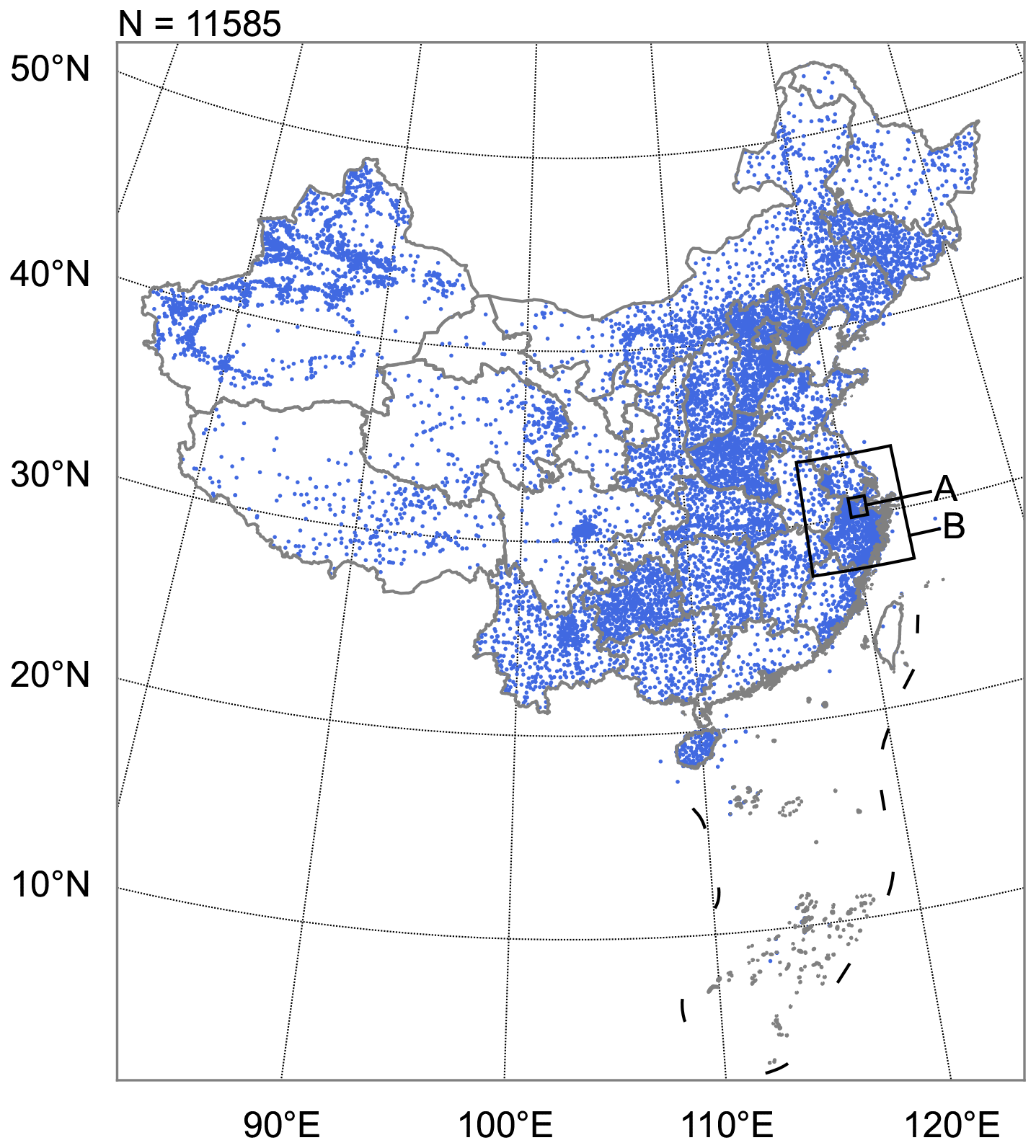
Figure 1 Spatial distribution of 11 585 weather stations providing pressure observations in this study in 2019. The smaller black box represents study domain A, covering 30 to 31° N and 120 to 121° E in Sect. 3.1, and the larger black box represents study domain B, spanning 27.3 to 33.3° N and 117.2 to 123.2° E in Sects. 3.2–3.3. Publisher's remark: please note that the above figure contains disputed territories.

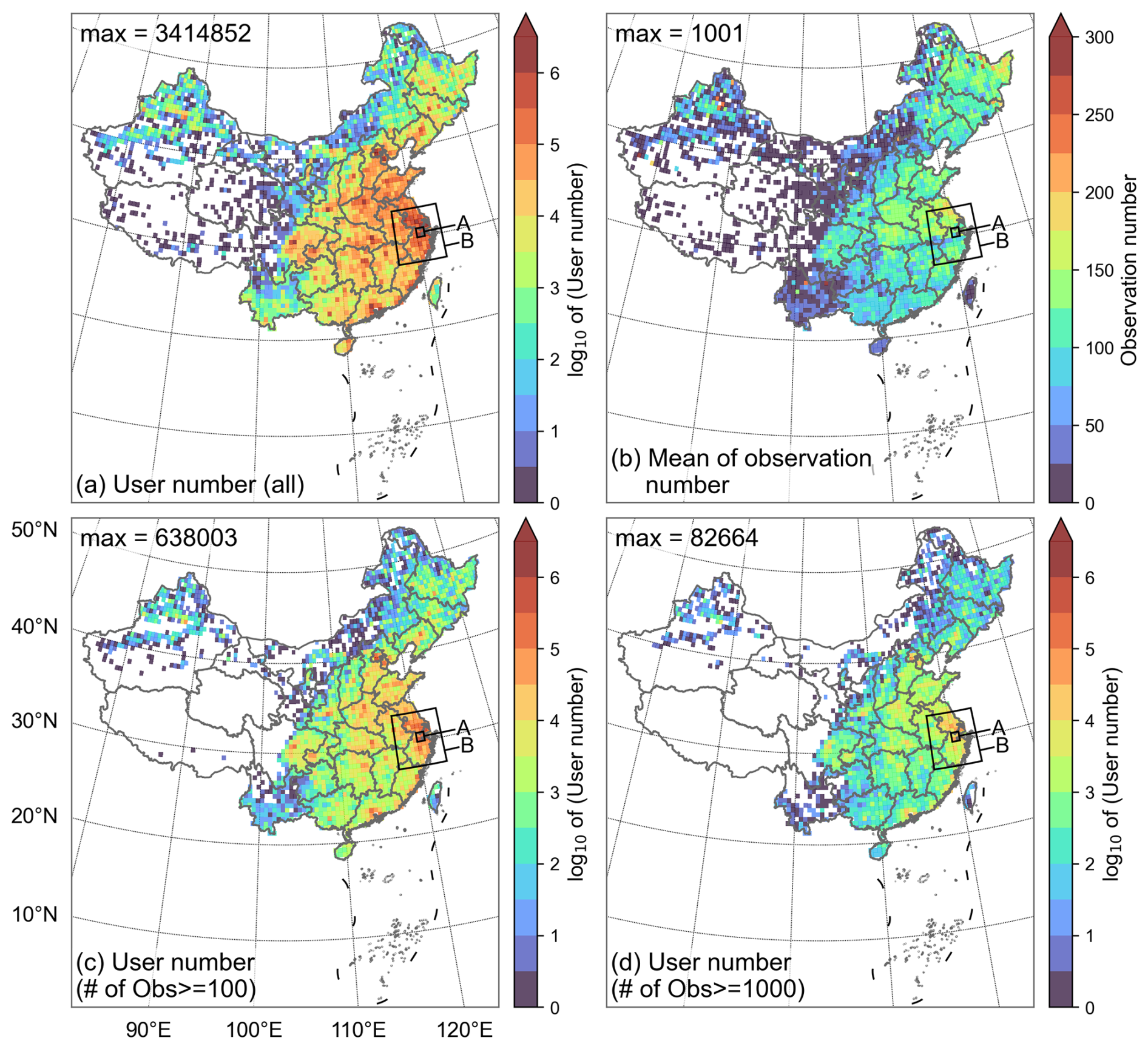
Figure 2 Spatial distribution of (a) the number of users contributing to smartphone pressure observations, (b) the average number of observations by users, (c) the number of users with more than 100 observations and (d) the number of users with more than 1000 observations in China during 2019. The data grid for the plots is 0.5°×0.5°. Users are assigned to locations where they have made their most frequent observations. The black boxes are the same as in Fig. 1. Publisher's remark: please note that the above figure contains disputed territories.

2.2 Spatial coverage ratio

In order to compare the spatial distribution of smartphone pressure observations under different conditions, this study defines the “spatial coverage ratio” of observations as follows. A region of any size is divided into a grid of 0.1°×0.1°. The proportion of the number of grid boxes containing smartphone observations to the total number of grid boxes in the region is defined as “smartphone coverage ratio”. The same methodology applies to the weather stations to define “station coverage ratio”.

2.3 TC cases

Three TC cases, namely Lekima in 2019, Hagupit in 2020 and In-fa in 2021, were selected from all landfalling TCs in China during 2019–2021. All three TCs passed through Zhejiang Province and Jiangsu Province (Fig. 3), both of which are densely populated regions. We focus on the super TC Lekima in 2019 in Sect. 3 to show the performance of the BC method. The method was also applied to Hagupit in 2020 and In-fa in 2021 for the TC MSLP analysis presented in Sect. 4.

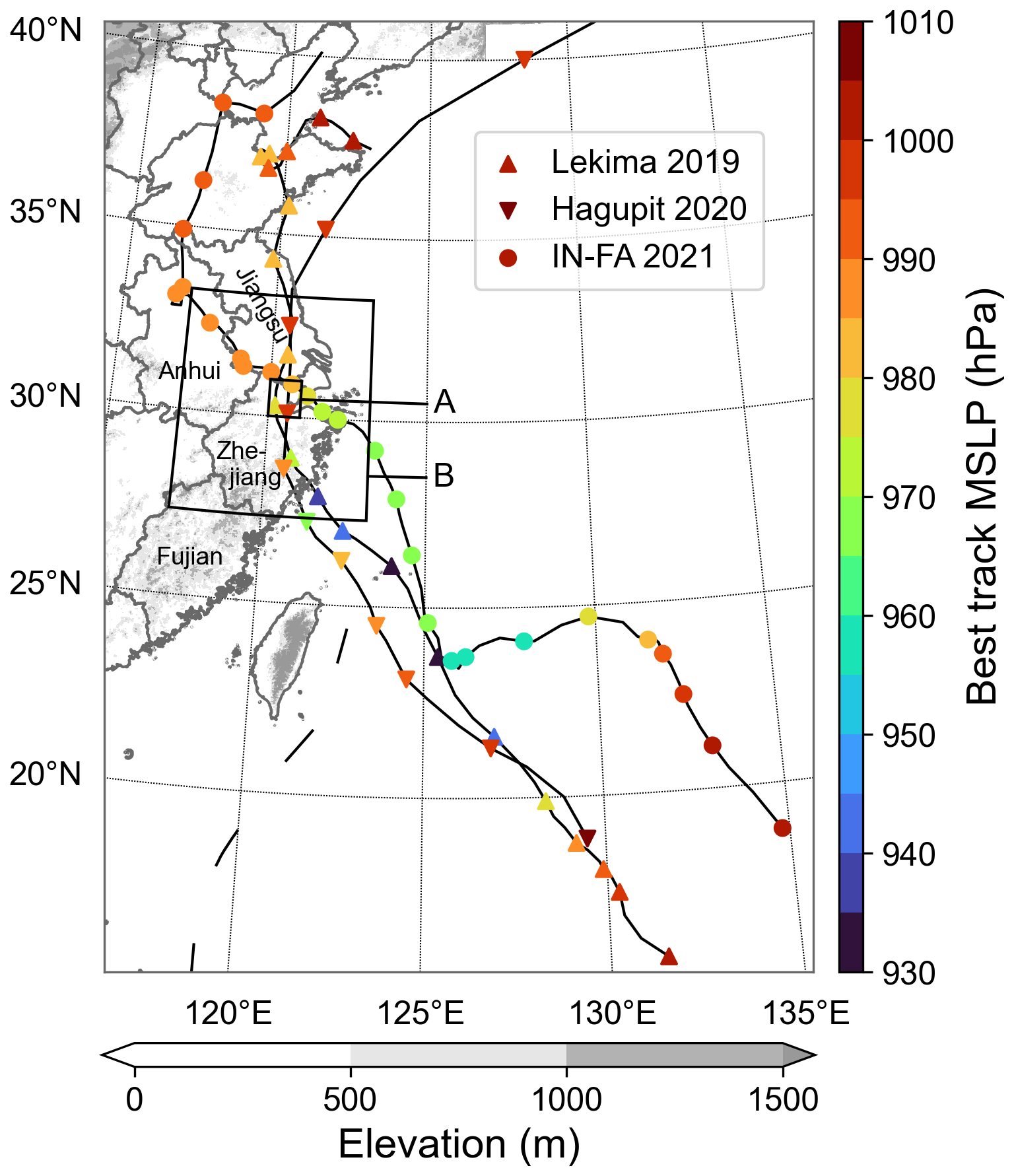
Figure 3 The tracks of TC Lekima in 2019, Hagupit in 2020 and In-fa in 2021 (marked every 3 h), with colors representing the MSLP at the TC center, according to STI best-track data. The gray shading indicates the elevation of the land surface. The black boxes are the same as in Fig. 1. Publisher's remark: please note that the above figure contains disputed territories.

TC Lekima was over the Chinese mainland from 9 to 11 August 2019. At the time of landfall, the MSLP from STI best-track data reached approximately 930 hPa. It then rose to 978 hPa when moving to the urban area of Hangzhou, Zhejiang Province. In this study, we take the area of 30–31° N, 120–121° E as study domain A and take an expanded area of 27.3–33.3° N, 117.2–123.2° E as study domain B (Figs. 1–3). Both domains cover the center of Lekima with a large number of smartphone observations. In domain B, between 10:00 LST on 9 August and 11:00 LST on 11 August 2019, 4 800 405 users in the research area contributed to the observations. The maximum number of observations is approximately 850 000 in a 0.1°×0.1° grid box. Compared to Lekima, Hagupit and In-fa experienced higher MSLPs. Moreover, In-fa traveled a longer distance over land than both Lekima and Hagupit did, contributing to greater temporal variations in the coverage ratios for both smartphones and weather stations.

3 Evaluation of MSLP correction by smartphone

3.1 Comparison with the BC method for unlabeled data

The methods for using machine learning to conduct the BC of smartphone data can be broadly categorized into two approaches: one for labeled data and the other for unlabeled data. Both methods use the differences from the reference sea-level pressures – in this study interpolated from weather station pressure data – as the variable to be corrected. The labeled data approach trains a model for all the pressure observations of each individual user (McNicholas and Mass, 2018), while the unlabeled data approach trains a model for all the smartphone sites in each grid element (Li et al., 2021) on a 0.1° (longitude) × 0.1° (latitude) grid in this study (Fig. 4). The performances of the two methods in the extreme-low-pressure environment of Lekima were compared over the area of 30–31° N and 120–121° E (domain A in Figs. 1–3). All pressure data during the TC landfall (from 00:00 LST on 9 August 2019 to 00:00 LST on 12 August 2019) were utilized as the test dataset, while the remaining data in 2019 were applied as the training dataset. Two random forest models for labeled and unlabeled data were built. Their descriptive variables and parameter settings are summarized in Tables 1 and 2, respectively.

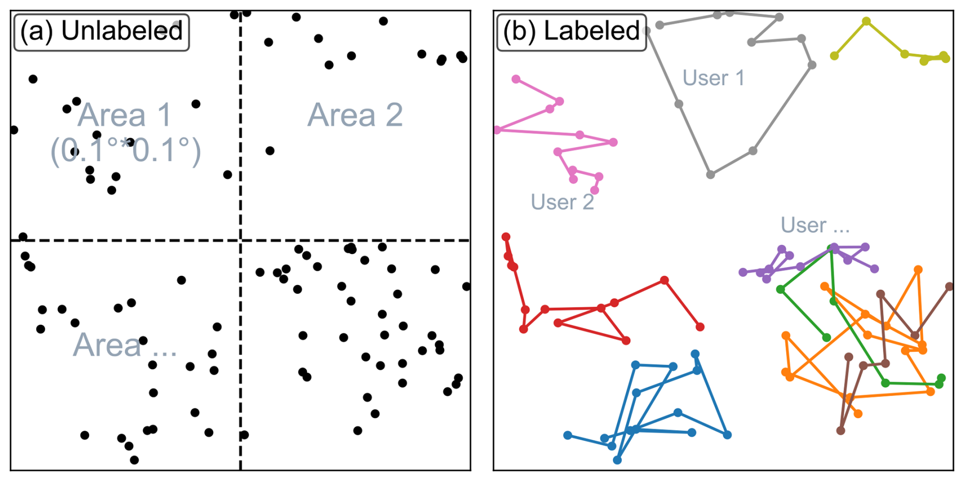
Figure 4 Schematic diagrams of models for (a) unlabeled data (to train a model for each “area” divided by dotted lines) and for (b) labeled data (to train a model for each “user” identified by different colors). In order to protect user privacy, the information in (a) and (b) is randomly generated and does not contain any user's real location information.

Table 1 Descriptive features of the two machine learning models.

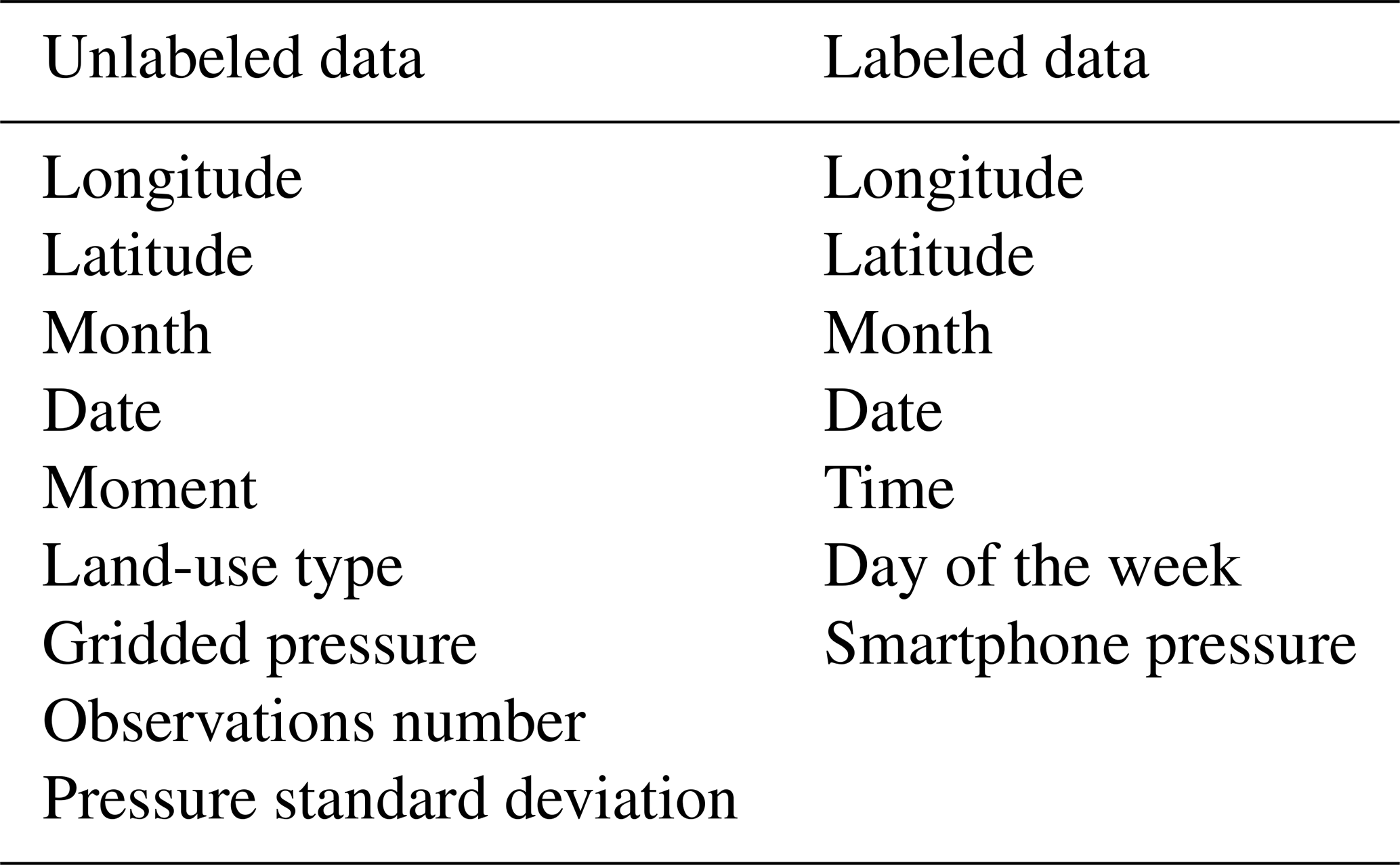
Table 2 Hyperparameter settings of the two machine learning models.

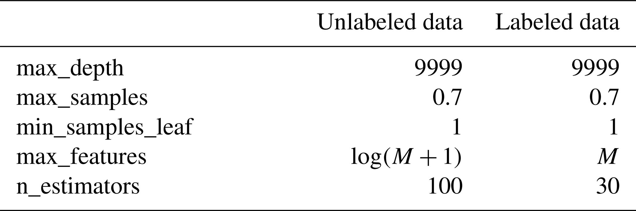
All parameters are from the function “RandomForestRegressor” of the scikit-learn machine learning library in Python (Pedregosa et al., 2011).
max_depth: the maximum depth of the tree (also known as “the base estimator”).
max_samples: the proportion of samples to draw from the training set to train each tree when bootstrapping.
min_samples_leaf: the minimum number of samples required to be at a leaf node.
max_features: the number of features to consider when looking for the best split.
M: the number of features used by the model.
n_estimators: the number of trees in the forest.

Smartphone pressures corrected by both models vary in trends similar to the surface pressure, with a general positive correlation between the pressures from smartphones and weather stations (Fig. 5). However, the corrected pressure with the unlabeled data approach clearly exhibits a significantly higher bias with a value of 4.521 hPa in contrast to 0.405 hPa for the labeled data approach. Moreover, the mean absolute error (MAE) and root mean square error (RMSE) from the BC on labeled data are also significantly lower, demonstrating that the labeled data approach for the BC of smartphone pressure performs superiorly in the low-pressure environment of TC Lekima.

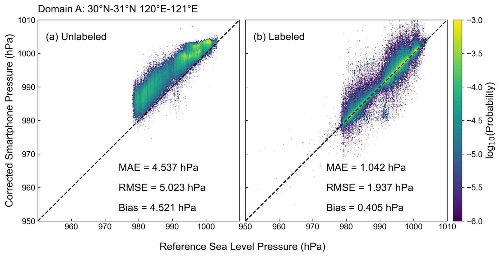
Figure 5 Probability distribution of the test data showing the correlation between the bias-corrected smartphone pressure and the reference sea-level pressure for (a) unlabeled data and (b) labeled data in domain A. The coloring represents the probability distribution using a base of 10 in every 0.1 hPa grid box. The dashed black line represents a perfect correlation.

Li et al. (2021) showed that the BC approach for unlabeled data successfully corrected the pressure data in a hailstorm case. We suspect that its poor performance for TC Lekima could have been related to the lack of strong TC samples in the training set. During non-TC periods, the most abnormal pressure observations occur when users are at high levels in tall buildings, resulting in low-pressure observations that require substantial corrections in the unlabeled data approach. These “fake” observations can reach the level of surface pressure at the center of a TC. When the training data lack strong TC samples, the machine learning model may use the high-altitude observations to correct the smartphone pressure near the ground during a TC, which can eventually lead to incorrect adjustment, resulting in values significantly higher than the reference sea-level pressure. In general, the unlabeled data approach can not discriminate between true and false low pressure. In contrast, however, the labeled data approach trains the machine learning model with the user's own historical observations (Fig. 4b), which are less uncertain in terms of altitude than observations from different users in a neighborhood. A single source of error makes machine learning models less prone to confusion between true low pressures and those falsely caused by high altitudes, thereby better adapting to unanticipated extreme conditions, such as super TCs.

Since the bias-corrected labeled data resulted in better correlation with the surface station data, they will be used in the subsequent analysis of all TC cases unless otherwise specified as unlabeled data.

3.2 Other quality control steps

In the previous section, we assumed that the pressure data from weather stations were accurate. However, the observations from weather stations are known to contain errors from unreliable stations. In this section, we use an expanded area covering 27.3–33.3° N and 117.2–123.2° E as the research domain (domain B in Figs. 1–3) because it includes a larger area of complex terrain. Considering that more stations in this larger region are located at high altitudes, which might introduce large errors in the interpolation of surface sea-level pressure, we selected only weather stations with altitudes of less than 100 m. The reference values at the smartphone locations were then generated from these selected stations. Applying the BC procedure for labeled data described in Sect. 3.1 to the large domain, the bias of smartphone data was reduced from 2.943 to −0.311 hPa. The low bias, primarily due to the observations at high altitudes (caused by users in tall buildings), has been greatly reduced (Fig. 6a and b). Furthermore, MAE decreases from 3.105 to 0.904 hPa and RMSE from 4.207 to 1.698 hPa.

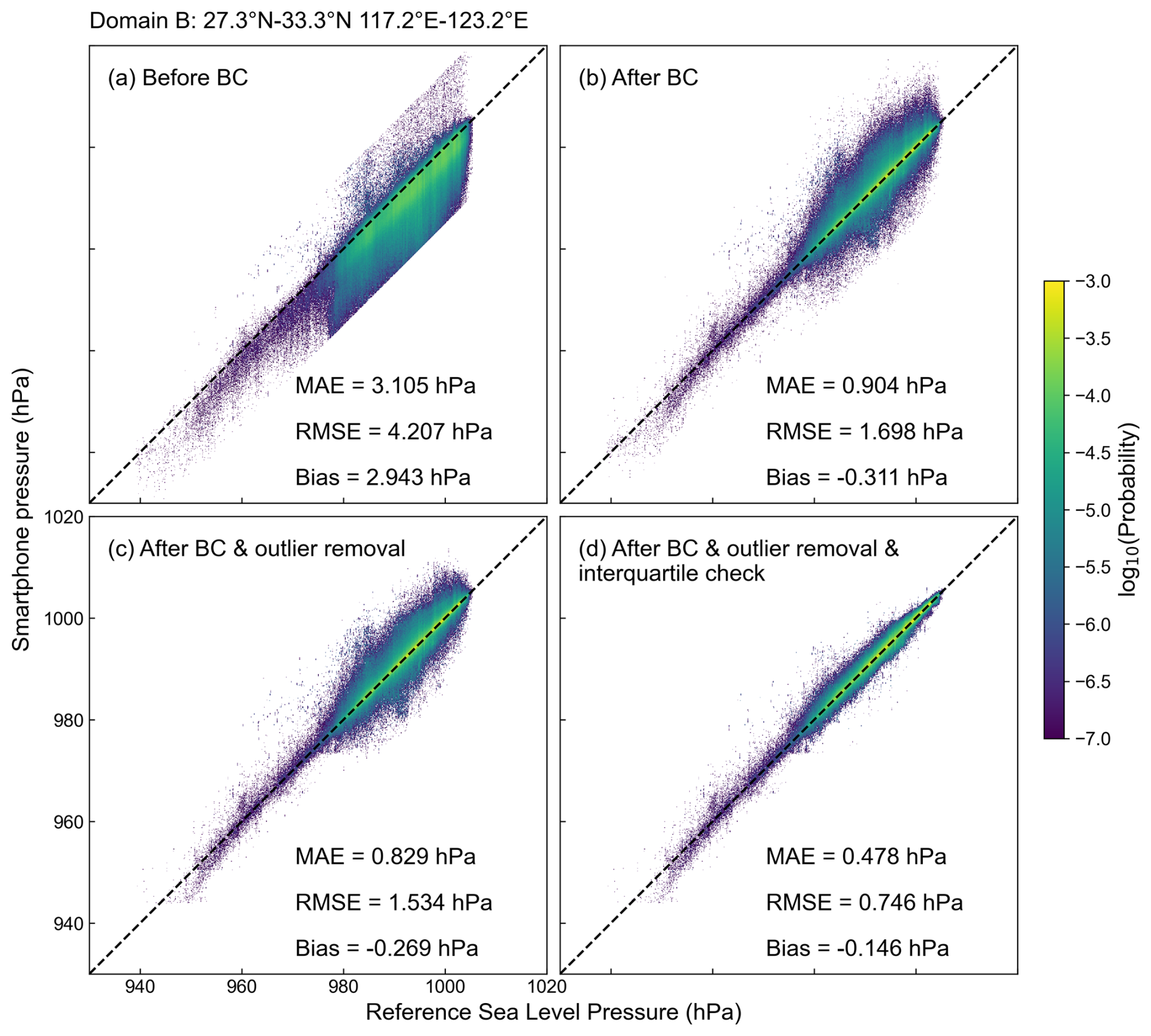
Figure 6 Same as Fig. 5, but only for labeled data (a) before BC, (b) after BC, (c) after outlier removal and (d) after interquartile check for domain B.

Eliminating outliers. The reference pressure generated by interpolating observations from the weather stations might be quite different from the true value given the large horizontal pressure gradient in TCs. This problem becomes more prominent for the expanded study domain that includes larger areas of complex terrain. Therefore, further actions of quality control are necessary. Station observations at any given time were considered outliers if the deviation from the mean pressure over domain B, or over the 20 nearest stations, is 3 times greater than the standard deviation in the same area. For this method to work, a sufficient number of observations from a single station is required. We thus selected 1070 weather stations that provided more than 70 % of the observations. The procedure was also applied to the bias-corrected smartphone data, which reduced the bias of smartphone observations to −0.269 hPa (Fig. 6b and c). To further reduce the bias, we applied the interquartile range method described below.

Interquartile check. For smartphone pressure observations, in every 0.5°×0.5° grid box we calculated the difference between the upper quartile and the lower quartile as the interquartile range (IQR). The smartphone observations that were 1 IQR higher than the upper quartile or lower than the lower quartile were considered outliers and removed. The quartile range method eliminated 13.8 % of the smartphone pressure data, reducing the bias from −0.269 to −0.146 hPa (Fig. 6c and d). The quality control procedure enabled the retention of the high-spatial-resolution characteristics while significantly improving the quality of the smartphone pressure data.

Figure 7 The workflow for smartphone pressure data quality control and bias correction.

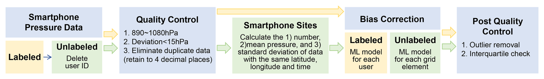
The workflow diagram shown in Fig. 7 summarizes the process of quality control and BC from the raw smartphone pressure data to the final data we used in the study.

3.3 Spatial distribution of smartphone pressure data

Using the smartphone pressure data after all quality control steps, we analyzed the horizontal distribution of sea-level pressure by combining both weather station pressure and smartphone pressure data in Domain B. The weather station observations are sparsely distributed throughout the region (Fig. 8a), whereas the substantially denser smartphone data cover the entire plain areas as well as some low-elevation areas (Fig. 8b). As a result, the smartphone pressure data reveal more details on the pressure distribution of TC Lekima. However, while the smartphone observations are densely distributed in the low-altitude areas, some weather station data from the high-mountain areas of southern Zhejiang, southern Anhui and northern Fujian are not represented in the smartphone data.

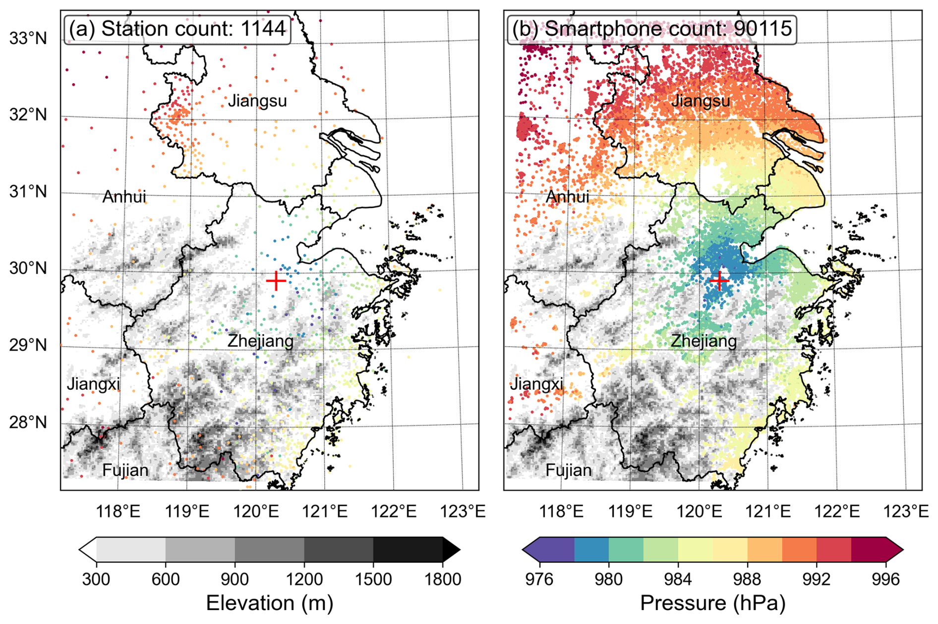
Figure 8 Distribution of (a) meteorological stations that measure pressure and (b) smartphone pressure observations in Domain B at 14:00 LST on 10 August 2019. The red “+” indicates the location of the TC center from the best track.

To examine the benefit of the high-resolution smartphone data in pressure analysis, we generated a sea-level-pressure analysis field based on only weather station observations (Fig. 9a) as well as one combining the weather station and smartphone observations (Fig. 9b).

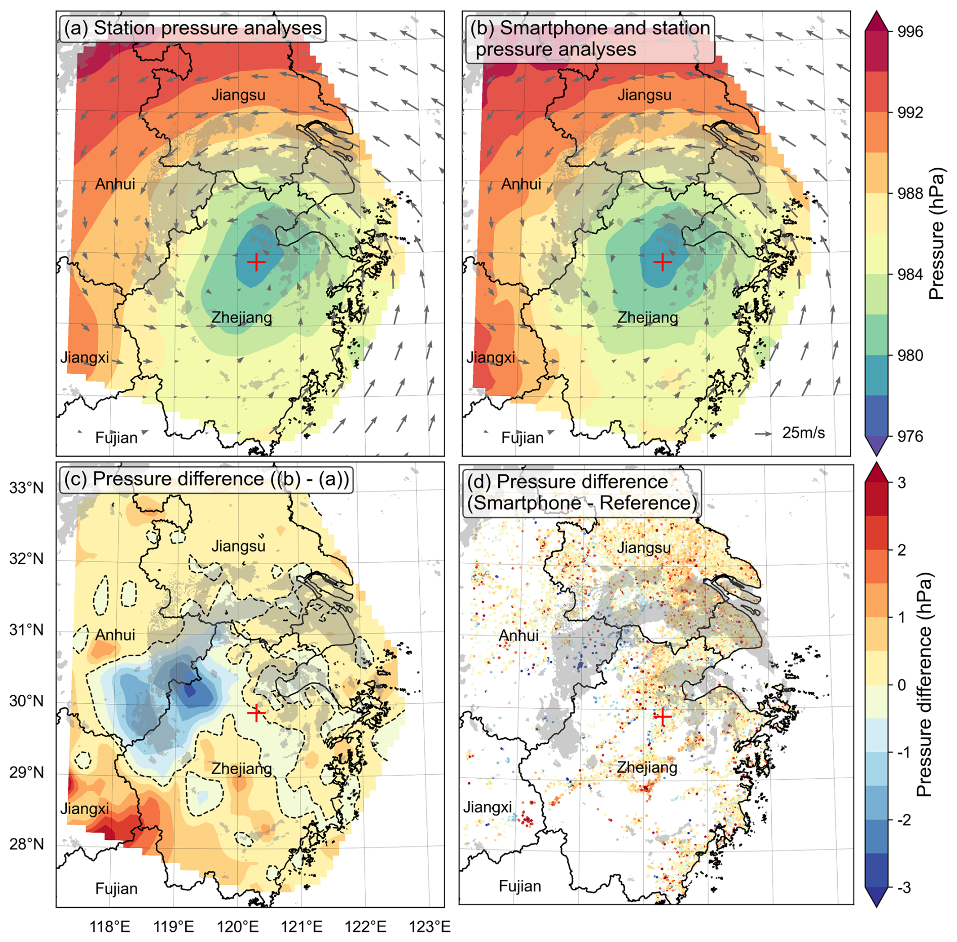
Figure 9 In Domain B at 14:00 LST on 10 August 2019, sea-level-pressure analysis field based on (a) meteorological station observations and (b) meteorological station and smartphone observations; (c) pressure difference between (b) and (a) and (d) between the corrected smartphone pressure and reference sea-level pressure. The gray shadings represent areas where radar reflectivity is higher than 30 dBZ, and the red “+” indicates the location of the TC center from best track. The arrows represent the wind field at the 925 hPa level from ERA5.

While the difference between the two analysis fields is widespread, the largest difference appears in the northwest of the Lekima center, where the analysis field with smartphone observations has lower sea-level pressure (Fig. 9c). The reason lies in the fact that the terrain in this area is complex and weather stations are sparse. In comparison, more smartphone observations are available, particularly in the valleys. Interestingly, the region of lower pressure coincides well with the southward extension of the spiral rainband as indicated by the radar reflectivity. This seems to suggest the analysis incorporating the smartphone data can reveal the mesoscale structure missed by the weather station analysis.

4 Improvement of TC MSLP estimate

Since the limited spatial resolution of weather stations makes it difficult to capture the true MSLP of landfalling TC, the MSLP in the best-track data usually differs somewhat from the lowest sea-level pressure observed by weather stations (Bai et al., 2021). The MSLP in the best track released by STI is mainly based on wind intensity (Fig. 10). Compared with weather stations, both the spatial coverage ratio and the resolution of smartphone observations are higher in areas with a relatively dense population, which may provide more accurate TC MSLP information. In this section, we explore whether smartphone pressure data can improve the estimate of MSLP in TCs using the three TC cases.

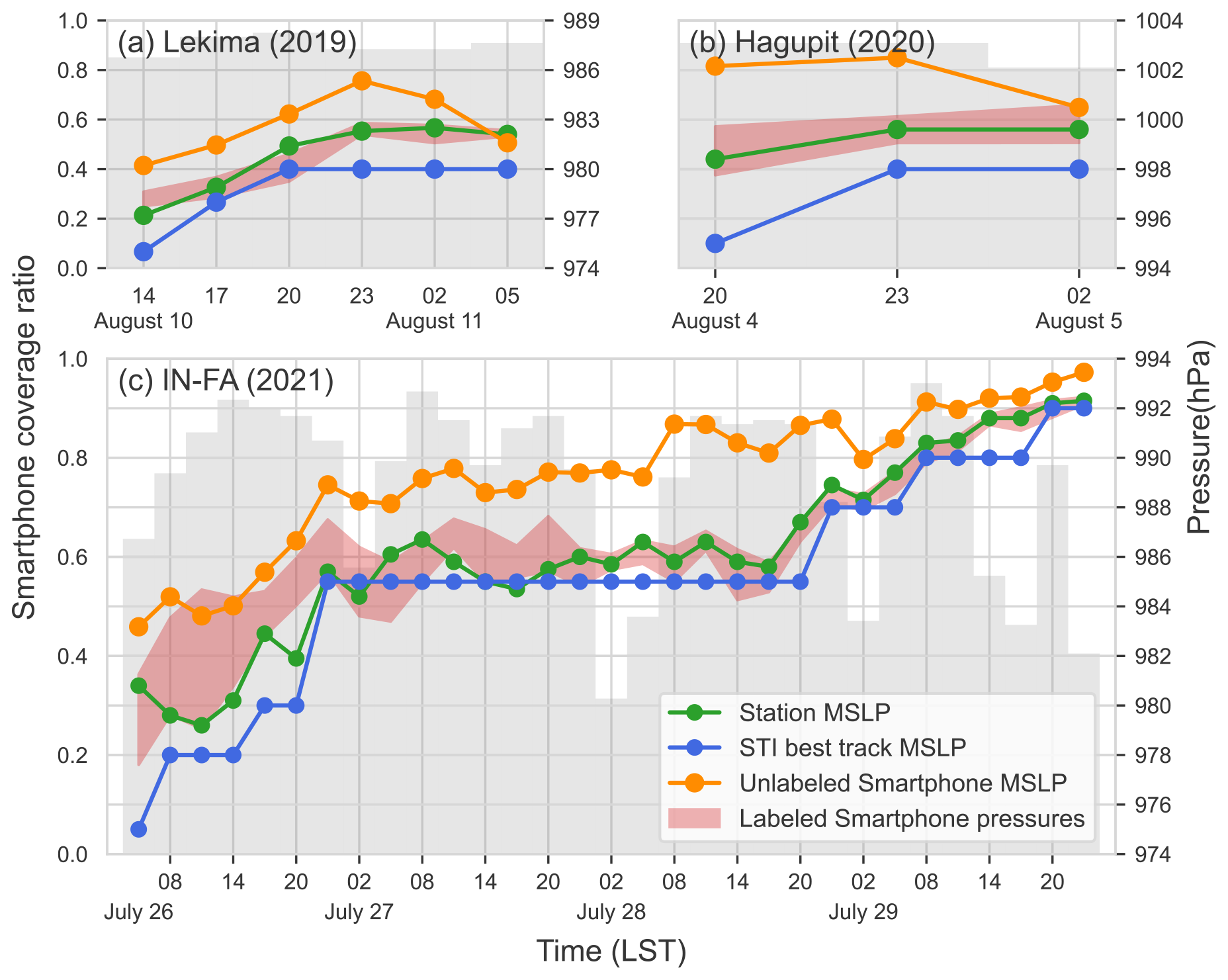
Figure 10 Variation in the MSLP and smartphone coverage ratio during (a) TC Lekima from 14:00 LST on 10 August to 05:00 LST on 11 August 2019, (b) TC Hagupit from 20:00 LST on 4 August to 02:00 LST on 5 August 2020 and (c) TC In-fa from 05:00 LST on 27 July to 23:00 LST on 29 July 2021. Green, blue and orange dots represent the MSLP from weather stations, STI best track and unlabeled smartphones, with a temporal resolution of 3, 3 and 6 h, respectively. Red shaded areas represent the lowest 10 % of labeled smartphone pressures. Gray bars represent smartphone coverage ratio. All the statistics were done in the area of 1.2°×1.2° around the TC center.

We selected the periods of relatively intensive observations, which spanned 6, 3 and 31 h, respectively, for Lekima, Hagupit and In-fa, to compare the MSLP estimate with those from the station and best track. The lowest station pressure and unlabeled smartphone pressure within a 1.2°×1.2° area of the TC center were taken as station MSLP, and unlabeled MSLP and the smartphone pressure, with the error margin of the lowest 10 % within the same area, were used as labeled smartphone MSLP (Fig. 10). The unlabeled MSLP clearly exhibits a significantly positive bias compared with both labeled and station MSLP, which is consistent with the previous conclusions. Most of the time, the station MSLP falls within the range of the labeled MSLP, and both are higher than that in the best track. The difference between the station MSLP and the best track is up to a substantial value of 2.76 hPa in Hagupit. Considering the small errors and deviations, as well as the generally high spatial resolution and coverage ratio of smartphone observations, it can be concluded that the best track generally tends to underestimate the TC MSLP.

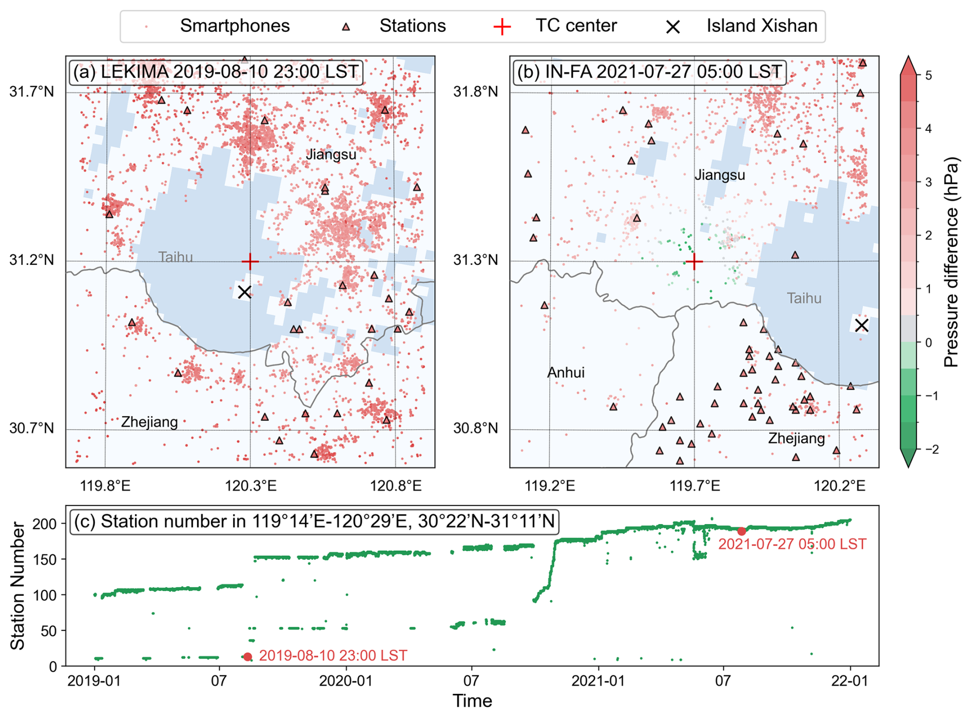
Figure 11 Distributions of weather station and smartphone observations from two examples during (a) TC In-fa and (b) TC Lekima in the area of 1.2°×1.2° surrounding the TC center. The coloring represents the difference between the pressure observations and the STI best-track MSLP. (c) Changes in the number of weather stations providing pressure observations from 2019 to 2021 at 119°14^′–120°29^′ E, 30°22^′–31°11^′ N (the geographical scope of Huzhou, Zhejiang Province).

The improvement of the MSLP estimate by smartphone observations depends on the location of the TC center. For instance, at 05:00 LST on 27 July 2021, during TC In-fa (Fig. 11a), when the TC center was positioned in an area with fewer stations but notably more smartphone observations, the smartphones estimated a lower pressure than that reported by the best track. In another instance (Fig. 11b), TC Lekima's center was located on a small island (denoted with “X”) in Lake Taihu, where there are no weather stations and measurements can only be made by smartphone. This highlights the advantages of crowdsourcing, which leverages the mobility and flexibility of individuals. Moreover, this instance happened to fall in a period when some stations with lower maintenance levels failed to measure and upload data steadily (Fig. 11c), which shows that smartphone pressure observations are valuable for filling some of the gaps created by unstable weather stations.

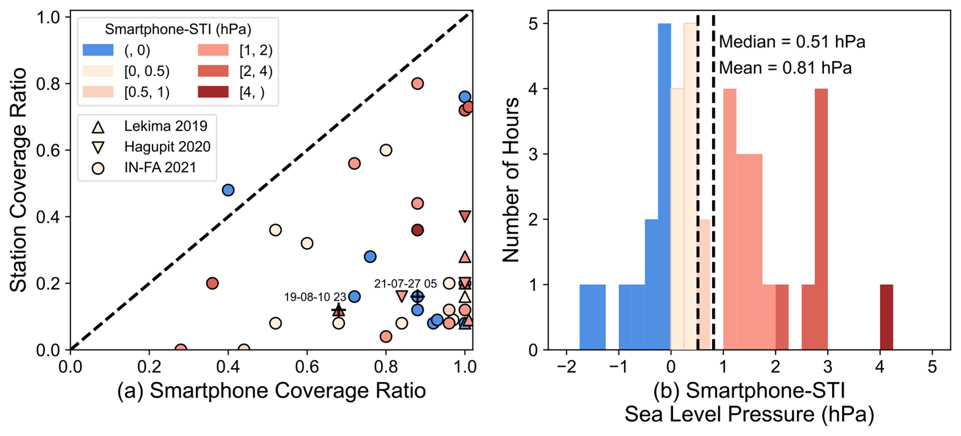
Figure 12 Comparison of smartphone MSLP with STI best-track MSLP for different spatial coverage ratios (defined in Sect. 2.2) for smartphones and weather stations (a) and PDF distribution (b). The squares, triangles and circles represent TC Lekima in 2019, TC Hagupit in 2020 and TC In-fa in 2021, respectively. The colors represent the difference between smartphone MSLP and STI MSLP indicated in the upper-left corner of (a).

Naturally, the smartphone's improvement in estimating MSLP heavily depends on smartphone and station coverage ratios. In the total of 40 time levels in our study, 39 exhibited a relatively higher smartphone coverage ratio compared to the station coverage ratio, indicating the advantages of smartphones in observing the pressure distribution around the TC center (Fig. 12). The larger number of smartphone observations around the TC center enabled a more accurate representation of the true pressure distribution. Overall, our analysis indicated that the STI MSLP underestimated the MSLP in 29 out of 40 instances, with a median difference of 0.51 hPa and an average of 0.81 hPa. This result highlights the limitation imposed by the low station coverage ratio, which may have caused the discrepancy between the STI MSLP and the smartphone MSLP.

5 Conclusion and discussion

In this study, we conducted bias correction of labeled smartphone pressure data in China using a machine learning scheme. Further, we analyzed the spatial distribution of sea-level pressure in three landfall TCs. The MSLP derived from smartphone observations was compared with that from the best-track data from STI.

We described two bias correction procedures, one for labeled and one for unlabeled data, which primarily differ in their methods of aggregating data samples in each situation. Upon applying these approaches to data from TC Lekima in 2019, we found that the labeled data approach resulted in smaller errors and deviations compared to the unlabeled data approach. Due to the high spatial resolution and extensive coverage, smartphone pressure data can supplement weather station pressure observations and improve pressure analysis in TCs.

Using data from TC Lekima in 2019, Hagupit in 2020 and In-fa in 2021, we compared the MSLP of TCs derived from smartphone data, weather station observations and the best-track dataset from STI. The smartphone and station MSLPs are generally in agreement, but the STI tends to underestimate the TC MSLP. Considering the higher resolution of smartphone observations, particularly in areas with sparse weather station coverage, and their minor errors after bias correction, it can be concluded that the smartphone pressure data can help estimate the intensity of TCs on land more accurately.

The conclusions of the three TCs provide valuable insights into the potential of smartphone pressure data for weather observation and forecasting. While the selection range of eligible TCs is relatively narrow due to the limited data amount of smartphone pressure observations, there is great potential for further research and application in this area. It is important to note that the research and application of smartphone pressure data are still in their early stages. However, by focusing on other types of weather systems and expanding the range of smartphone data collection, we can develop the utilization value of the limited smartphone data in more dimensions. Additionally, although waiting for data accumulation is an essential aspect of future research, the increasing use of smartphones offers promising potential for data collection.

Although the average number of user observations is currently low, there is potential for improvement. Kim et al. (2015) found that the amount of smartphone pressure data generated by weather apps decreased significantly after the publicity period ended, indicating that the enthusiasm of the public to participate in mobile weather observation needs to be fundamentally improved. By helping the public understand the role of smartphone data in weather observation, forecasting and warning, we can increase enthusiasm for mobile weather observation. Citizen science projects such as PressureNet (2024) and Zooniverse (2024) provide good examples of how to engage the public in weather data collection, and these practices should be implemented more widely in other countries and regions.

In conclusion, while there are challenges in the utilization of smartphone pressure data, there is great potential for further research and application. By addressing these challenges and engaging the public in mobile weather observation, we can improve the spatial and temporal resolution of the data to enhance their value for weather forecasting and warning systems. The future of smartphone pressure data in meteorology is promising, and with continued research and public engagement, we can unlock its full potential.