Validation and comparison of cloud properties retrieved from passive satellites over the Southern Ocean

The clouds over the Southern Ocean (SO) play a vital role in defining the Earth's energy budget. The cloud properties over the SO are known to be different from their Northern Hemisphere counterparts. As a result, monitoring cloud properties over the SO, including macro- and microphysical properties, is of particular interest.

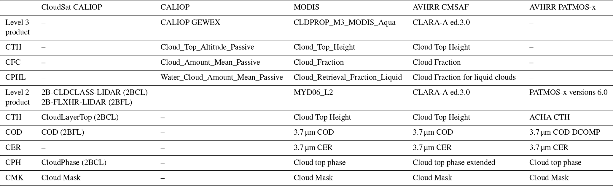
We compared the Level 3 products from AVHRR CMSAF, MODIS, and CALIOP for cloud top height, cloud fraction, and cloud liquid fraction. The study found that MODIS underestimated cloud top heights, while AVHRR CMSAF overestimates them when compared to Level 3 CALIOP. The overall cloud cover for MODIS was less than that of CALIOP while AVHRR CMSAF showed higher cloud cover over mid-latitudes and lower cloud cover over land in the Level 3 product. The comparison of cloud fraction for liquid clouds against CALIOP indicates that AVHRR CMSAF tends to overestimate, whereas MODIS tends to underestimate the liquid cloud fraction. The magnitude of the difference varies with the latitude and season.

Following the Level 3 analysis, we investigated three passive remote sensing satellite datasets, MODIS Collection 6.1, AVHRR CMSAF CLARA-A3, and AVHRR PATMOS-x, over the SO. We validated the Level 2 cloud mask, the cloud top height, and the cloud phase for 2015 retrieved from the passive sensors with active CloudSat-CALIOP sensors. We compared the effective radius and cloud optical depth amongst the three passive sensor datasets.

This research found that there are substantial uncertainties in the cloud top height, the cloud optical depth, and the cloud thermodynamic phase, over the SO. The extent of which varies depending on the cloud property and retrieval algorithm used. The cloud mask comparison revealed varying levels of agreement between passive and active sensor observations, with a Kuiper Skill Score (KSS) of 0.71 (AVHRR CMSAF), 0.70 (MODIS), and 0.43 (AVHRR PATMOS-x). In the comparison of cloud top height, a mean absolute bias of 0.65 km (AVHRR CMSAF), 1.03 km (MODIS), and 1.27 km (AVHRR PATMOS-x) was observed for single-layer cloud scenes cases. This mean absolute bias increased to 1.87 km (AVHRR CMSAF), 3.25 km (MODIS), and 3.30 km (AVHRR PATMOS-x) for the multilayered cloud scenes. In the comparison of cloud effective radius, it was observed that the disagreement between the passive sensors was more significant in the presence of multilayer clouds. The effective radius disagreement was higher for ice clouds. Variations in ice habit assumptions, lookup table configurations, and phase classification schemes could contribute to these differences. We found that the presence of sea ice strongly influences the retrieval of cloud optical depth at high latitudes, with most passive optical depths higher over sea ice than over ocean. The new finding that contradicts previous studies may result from the difficulty of retrieving cloud optical depth over ice using the retrieval algorithms.

1 Introduction

The role of clouds is vital to the Earth's energy budget. The Southern Ocean (SO) is one of the cloudiest places on the planet. Climate simulations and reanalyses (Trenberth and Fasullo, 2010; Schuddeboom and McDonald, 2021; Zelinka et al., 2020) over the SO show a persistent negative bias in shortwave (SW) radiation and an overestimation of the outgoing longwave (LW) radiation. Schuddeboom and McDonald (2021) compared Coupled Model Intercomparison Project Phase 6 (CMIP6) simulations with satellite data and identified substantial discrepancies in the representation of clouds, particularly with low-level clouds. This inconsistency leads to the simulations exhibiting an inverse correlation between the mean and compensating errors of SW cloud radiative effects (CRE), which is prevalent over the SO. Zelinka et al. (2020) examined the climate sensitivity of 27 CMIP6 global climate simulations and found that the previous climate models had made the SW low cloud feedback component stronger. They found that a substantial shift in the SW cloud feedback from high-latitudes in the Coupled Model Intercomparison Project Phase 5 (CMIP5) models to extratropics has occurred in the CMIP6 models, especially over the SO. The uncertainty in the models demonstrates a need to better understand the Southern Ocean atmospheric and ocean properties, particularly cloud properties.

Compared against the clouds over the North Atlantic and the North Pacific, SO clouds have a higher probability of cloud glaciation (Davies et al., 2017), and the increased presence of supercooled liquid water (Huang et al., 2015; Morrison et al., 2011; Ovarlez et al., 2002). Davies et al. (2017) examined the plane parallel albedo bias, and concluded that SO clouds have a smaller heterogeneity bias than those over the Northern Hemisphere. Hu et al. (2010) examined Cloud-Aerosol Lidar with Orthogonal Polarisation (CALIOP; Young et al., 2008) observations and discovered that the supercooled liquid water retrieval at mid-latitudes, is dependent on the cloud top temperature and cloud top height, and that supercooled water clouds were more common over the SO. Huang et al. (2015) compared clouds over the North Atlantic against those over the SO, using a merged radar-lidar product and discovered that the presence of boundary layer clouds and mid-level clouds, with smaller droplet sizes was more prevalent over the SO. Mace et al. (2009) employed a merged radar-lidar product, to demonstrate that mid- and low-level multilayer clouds are present in more than half of the scenes over the SO (poleward of the ocean polar front), which is more frequent than their North Atlantic and Pacific counterparts. In a study conducted using upper air soundings from a collection of SO field campaigns, Truong et al. (2020) found the presence of multilayer clouds in over half the scenes over the high-latitudes of the SO. Further investigation uncovered a bias in the thermodynamic structure, specifically the frequency of the occurrence of multilayer clouds, in the ECMWF's fifth-generation atmospheric reanalysis (ERA5) (Truong et al., 2022) over the Southern Ocean. ERA5 more commonly simulated relatively thick single-layer clouds than inferred from the soundings. They demonstrated that the radiative transfer through these clouds is sensitive to cloud macrophysics, as thin multilayer clouds can help reduce downward shortwave surface radiation over the SO. These findings highlight the unique characteristics of SO, and a need to understand the influence of multilayer clouds in retrieving cloud properties over the SO.

Previous research on cloud property retrievals, revealed a dependency on the presence of multilayer clouds for CRE retrievals, which was further reinforced in studies such as L'Ecuyer et al. (2019), Hinkelman and Marchand (2020) and Yost et al. (2023). L'Ecuyer et al. (2019) concluded that multilayer clouds contribute to enhancing LW radiation by 10.4 W m⁻² and reducing SW radiation by 22.3 W m⁻² and are often misclassified as single-layer, thick, mid-level clouds, leading to global CRE biases. Hinkelman and Marchand (2020) evaluated the Clouds and the Earth's Radiant Energy System (CERES, Minnis et al., 2020) observations and Cloud-Aerosol Lidar with Orthogonal Polarisation (CloudSat) CALIOP data (Sassen et al., 2008; Wang et al., 2013) against field observations from Macquarie Island Cloud and Radiation Experiment (MICRE; Marchand, 2020). They observed a bias of $-\mathrm{10}\mathrm{W}{\mathrm{m}}^{-\mathrm{2}}$ in LWCRE and concluded that the factors contributing to this bias include low clouds, multilayer clouds, and precipitating clouds. The CERES Visible Infrared Imaging Radiometer Suite (VIIRS) observations were evaluated against CALIOP observations by Yost et al. (2023) and the re-evaluation showed that multilayer clouds are one of the main contributors to errors in cloud top height retrieval.

Previous studies have conducted regional analyses to resolve some of the uncertainties over the SO, either typically emphasising comparisons with land observations, or focusing on single satellite records (Ahn et al., 2018; Hinkelman and Marchand, 2020; Kang et al., 2021; McFarquhar et al., 2021; Xi et al., 2022). In recent years there have been several field campaigns over the SO: such as Clouds Aerosols Precipitation Radiation and atmospheric Composition over the Southern Ocean (CAPRICORN; McFarquhar et al., 2021) I and II; the Southern Ocean Clouds, Radiation, Aerosol Transport Experimental Study (SOCRATES; McFarquhar et al., 2021); Measurements of Aerosols, Radiation, and Clouds over the Southern Ocean (MARCUS; McFarquhar et al., 2019, 2021); and MICRE. Ahn et al. (2018) compared cloud phase retrieved between Moderate Resolution Imaging Spectroradiometer (MODIS, Menzel et al., 2008), CALIOP, and in-situ observations and found that mixed-phase clouds are often underestimated by the satellite observations. Xi et al. (2022) also observed that the presence of mixed phases clouds dominated the MARCUS campaign observations. Kang et al. (2021) examined MODIS, CERES and Himawari satellite observations against SOCRATES field observations. They found that a low bias of the cloud effective radius is due to compensating errors between non- or lightly precipitating cases and heavily precipitating cases. Despite these campaigns, the lack of long-term data continuity and spatial coverage remains a challenge.

Satellite observations are one of the primary tools for monitoring the weather and climate globally and are particularly important over the remote SO, where in-situ observations are sparse. Satellite instruments, such as Advanced Very-High-Resolution Radiometer (AVHRR; Pavolonis and Heidinger, 2004), have been making observations since the early 1980s, which, if sufficiently stable and accurate, could begin to provide information on the cloud response to a changing climate. Passive satellite cloud retrieval forward models typically assume a single-layer cloud. This results in large negative biases for retrievals of cloud top height particularly in the presence of multilayer clouds. Hence in this paper, we focus on the quality of satellite retrievals over the SO.

In this study, we analyse three well-known global passive satellite datasets: AVHRR Pathfinder Atmospheres-Extended (PATMOS-x, Heidinger et al., 2014), AVHRR Satellite Application Facility on Climate Monitoring (CMSAF; Karlsson et al., 2023b), and MODIS (Menzel et al., 2015) over the SO. We validate the cloud top height (Sect. 4.2.3) and mask (Sect. 4.2.2) with merged CloudSat CALIOP data, and compare the cloud phase and effective radius (Sect. 4.2.4). We perform the analysis at the monthly level (L3) in Sect. 4.1, followed by an in depth analysis into instantaneous observations (L2) in Sect. 4.2. The results are analysed separately for single and multilayer clouds and a case study illustrates the main findings (Sect. 4.2.1).

2 Data

The analysis considers cloud information from two different satellite instruments MODIS and AVHRR and 3 different algorithms/data providers. Active satellite instruments CloudSat-CALIOP, are used to validate the data. A brief overview of all the datasets used is given below.

2.1 CloudSat-CALIOP P1 R05

The CloudSat and Cloud-Aerosol Lidar and Infrared Pathfinder Satellite instruments (CALIPSO), were launched in April 2006. The satellites are part of the NASA Afternoon Constellation, known as the A-train, a coordinated group of satellites crossing the equator from south to north within seconds of each other in an afternoon orbit. CloudSat exited the A-train in February 2018, to a lower orbit, due to technical difficulties, and CALIPSO rejoined it in September 2018 to form the C-Train. CALIPSO officially ceased its operation in September 2023, while CloudSat was switched to daytime-only observations in December 2021 and deactivated in December 2023. CloudSat (Stephens et al., 2002) uses the Cloud Profiling Radar (CPR) to observe the vertical profiles of the clouds. The CPR onboard CloudSat has a vertical resolution of 500 m and horizontal resolution of 1.4 km operating at W-band (94 GHz). CALIPSO (Winker et al., 2003; Young et al., 2008) uses CALIOP, a lidar with two wavelengths of 532 and 1064 nm, to measure vertical profiles of cloud and aerosol. The CALIOP GEWEX cloud product (NASA/LARC/SD/ASDC, 2019), is the L3 product derived from temporal averaging of 5 km cloud merged layer products version 4, for a month.

The merged CloudSat-CALIOP product, is obtained from collocating the observations from both the CPR and CALIOP instruments. The temperature profile for the merged product is obtained from the European Centre for Medium-Range Weather Forecasts (ECMWF), and MODIS radiance data is used as supplementary information for cloud classification. The dataset is made available by the Cooperative Institute for Research in the Atmosphere (CIRA), Colorado State University. The CloudSat-CALIOP merged dataset includes the L2 retrieved cloud property data, and is provided under different product names for different cloud and radiation properties. In this study, we have used the 2B-CLDCLASS-LIDAR (Sassen et al., 2008; Wang et al., 2013), 2B-FLXHR-LIDAR (Henderson et al., 2013; L'Ecuyer et al., 2008; Henderson and L'Ecuyer, 2023) and the 2B-CWC-RVOD products (Leinonen et al., 2016). The 2B-CLDCLASS-LIDAR (hereby known as 2BCL) combines the advantages of LIDAR and RADAR to get an understanding of cloud vertical profile, cloud classification and cloud properties such as cloud top height (CTH), cloud base height (CBH) and cloud phase (CPH). The 2B-FLXHR-LIDAR (hereby known as 2BFL) retrieval product provides the broadband fluxes and heating rates from the CloudSat-CALIOP observations, which are useful in understanding the flux rates and optical depth of the clouds. The data products are available throughout the day for CTH, however, the revisit time is 16 d. The L2 data product with a spatial resolution of 5 km for 2015 is used for this comparison. For the climatology of 7 years (2009–2016), L3 monthly data from CALIOP, CAL_LID_L3_GEWEX_Cloud-Standard-V1 is used.

2.2 Moderate Resolution Imaging Spectroradiometer (MODIS)

The AQUA satellite, with the MODIS sensor onboard, was launched in 2002 and is also part of the A-train. The instrument has 36 spectral bands (wavelengths 0.4–14.4 µm). Every five minutes, the MODIS sensor scans an area of 2330 km². The MODIS-AQUA L3 monthly data product CLDPROP_M3_MODIS_Aqua (Platnick et al., 2019) is used for the analysis of L3 data. The data include cloud properties such as CTH, cloud fraction (CFC), cloud optical depth/thickness (COD/COT) and cloud effective radius (CER). MYD06_L2 (hereby known as MYD; Platnick et al., 2015a) contains data products retrieved from the MODIS instrument on the AQUA platform. The L2 data consist of 1 km resolution pixels, with cloud microphysical properties and 5 km resolution for all other retrieved properties. The MYD 1 km retrieval, classifies pixels as cloudy and partially cloudy. We have considered clear, cloudy and partially cloudy for our analysis. The MYD collection uses the CO₂ slicing method and the Infrared Window Approach (IRW) to retrieve cloud top properties (Menzel et al., 2015).

2.3 Advanced Very-High-Resolution Radiometer

The AVHRR instrument is a broadband radiometer with six spectral channels spanning the visible, near‑infrared, and infrared regions, of which only five can be transmitted at any given time. The instrument is a cross-tracking scanning radiometer with a resolution of 1.1 km. The AVHRR instrument was first launched in late 1978, and has since been operated continuously onboard National Oceanic and Atmospheric Administration (NOAA) Polar Operational Environmental Satellites (POES), and more recently onboard the European MetOp platforms. The NOAA-19 satellite is used for the L2 analysis.

2.3.1 AVHRR CMSAF

CLARA-A3 (The CMSAF Cloud, Albedo and Surface Radiation dataset from AVHRR data – third edition) is a climate data record derived from the polar-orbiting AVHRR instrument, of cloud properties, surface albedo, and surface radiation budget products for the period 1979–2024 (45 years; Karlsson et al., 2023c). The major advantage of this dataset is the global coverage and the time-period available for analysis. The CLARA-A3 edition (Karlsson et al., 2023b) contains retrieved cloud properties such as CTH, CPH and cloud water path (CWP). The CLARA-3 dataset is available for instantaneous, daily, and monthly periods and was released in mid-2023. The data used in the analysis have a spatial resolution of 5 km. The CLARA A3 uses an artificial neural network (ANN), trained on collocated AVHRR-CC data (Håkansson et al., 2018) to obtain cloud-top height. In the case of cloud microphysics, traditional retrieval methods look-up tables (LUTs) are created based on Nakajima and King (1990).

2.3.2 AVHRR PATMOS-x

The AVHRR PATMOS-x provides a climate record of atmospheric cloud properties and brightness temperatures retrieved by merging the information from AVHRR, and the collocated High-resolution Infra-Red Sounder (HIRS, Foster et al., 2023). The algorithm was developed by the NOAA and the Cooperative Institute for Meteorological Satellite Studies (CIMSS). The climate data record covers a period of 44 years (1979–2023), with a resolution of 0.1°×0.1° grid globally (Foster et al., 2023). The dataset includes CTH, CER, COD, and ice water path (IWP). Multiple algorithms are referenced in the product, in particular the Advanced Baseline Imager Cloud Height Algorithm (ACHA; Heidinger, 2011), MODIS CO₂ slicing algorithm (Menzel et al., 2008), and Daytime Cloud Optical and Microphysical Properties (DCOMP; Walther et al., 2013). In this study, the ACHA CTH algorithm uses 11 and 13.3 µm observations along with the split-window approach (Heidinger and Pavolonis, 2009), and data from the AVHRR Extended (CLAVAR-x). When AVHRR is combined with HIRS information, the CO₂ CTH can be determined.

2.4 Validation of polar satellites over the Southern Ocean

There have been numerous validation studies which we summarise here. Common to most studies, the validation results are generally reported for cloud globally and not as a function of specific regions. Validation of the cloud products over the SO has been mostly performed using monthly data.

The MODIS products have been compared against CALIOP in several studies. Holz et al. (2008) found that CTH is underestimated by MODIS by 1.4±2.9 km globally, when compared with the 1 km CALIOP product. In the case of the 5 km CALIOP product, the difference is $-\mathrm{2.6}\pm \mathrm{3.9}\mathrm{km}$. Yang et al. (2021) compared the CTHs of MODIS AQUA, MODIS TERRA, CALIOP, CloudSat and the Advanced Himawari Imager on Himawari-8 (HW8), with ground-based Ka-band zenith radar (KAZR), at the Semi-Arid Climate and Environment Observatory of Lanzhou University (SACOL) site in NW China. They observed that the smallest mean CTH differences between passive satellite sensors and KAZR are −0.35 km (−0.88 km for multilayer) for MODIS Terra, −0.87 km (−1.58 km for multilayer) for MODIS Aqua and −0.69 km (−1.70 km for multilayer) for Himawari-8 (HW8).

Karlsson and Johansson (2013) compared the CLARA-A1 (The CMSAF, Cloud, Albedo and Surface Radiation dataset from AVHRR, data-edition one) dataset with CALIOP observations, and found that the overall bias in the CTH changes with the optical depth of the cloud with biases increasing as COD decreases (<0.35). The study also inferred that the CTHs of high clouds (>8 km) are underestimated and boundary layer clouds (<2 km) are overestimated. Additionally, the research highlighted a substantial underestimation of cloudiness in polar regions, particularly during the polar winter.

Foster et al. (2023) found that AVHRR PATMOS-x Version 6, has improved the performance of cloud property retrievals, especially across the polar region from the previous version. The cloud fraction increased by 3 % from Version 5 to Version 6, although the variation and seasonality of cloud optical depth across the satellite data decreased.

Karlsson and Devasthale (2018) evaluated four global cloud climate records, the International Satellite Cloud Climatology Project (ISCCP), European Space Agency (ESA) Climate Change Initiative (CCI) V3, CLARA-A2 and PATMOS-x V5, against each other and a CALIPSO dataset. The study uncovered large biases in cloud cover, notably in the southern polar region, with major differences between the PATMOS-x and CLARA-A2 datasets in the cloud fraction. The PATMOS-x gives similar cloud amounts when compared to CALIOP observations. Furthermore, indications of orbital drift phenomena were detected in the PATMOS-x dataset, which was linked to the changing solar zenith and solar azimuth angle and surface temperatures resulting in increased cloud amount detection.

Chang et al. (2010) studied all the retrieval methods for CTHs from the Twelfth Geostationary Operational Environmental Satellite (GOES-12) data, and found that there exists a negative bias of 2.5 km±1 km for all CTHs retrieved as two-layer and 4.5 km±2 km for cases with more than two layers. Sourdeval et al. (2016) found that the IWP retrieval quality can be impacted by multilayer clouds and proposed an IWP retrieval method for multilayer conditions. They statistically analysed the results to conclude that the new method is successful for retrieving IWPs ranging from 0.5–1000 g m⁻².

2.5 Multilayer clouds and detection algorithms

Mace et al. (2009) used the CloudSat-CALIPSO product to show that mid- and low-level multilayer clouds are present in more than half of the scenes over the SO (along the ocean polar front), which is more often than their Arctic counterparts. Similar studies, have found that ignoring the multilayer structure of clouds can lead to errors in the retrieval of cloud properties such as cloud top pressure, cloud optical depth, and cloud fraction (Chen et al., 2000; Heidinger and Pavolonis, 2005; Joiner et al., 2010). L'Ecuyer et al. (2019) found that the multilayer clouds contribute to enhancing LW radiation by 10.4 W m⁻² and reducing SW radiation by 22.3 W m⁻², and they are often misclassified as single-layer thick mid-clouds leading to global CRE of $-\mathrm{17.1}\mathrm{W}{\mathrm{m}}^{-\mathrm{2}}$. The study also confirmed that the discrepancy in radiative fluxes, indicates that clouds with similar top of the atmosphere radiative signatures can have varying impacts at the surface and on atmospheric heating.

Several multilayer cloud detection algorithms for global satellite instruments using visible to infrared bands have been developed (Baum et al., 1994; Joiner et al., 2010; Kawamoto et al., 2002). In general, the multilayer detection algorithms are limited to thin-cirrus over low clouds, ocean areas or two-layer retrieval systems (Joiner et al., 2010; Sun-Mack et al., 2006). MODIS, AVHRR, CERES have used CALIOP datasets to train decision tree algorithms to refine the multilayer cloud detection algorithms (Li et al., 2011; Marchant et al., 2020; Sun-Mack et al., 2006; Simpsom et al., 2001).

In the multilayer detection flag for MODIS MYD (Level-2 data; Marchant et al., 2020), the multilayer classification agreement with CloudSat-CALIOP merged product is only 34 % (Wang et al., 2016). New Artificial intelligence (AI) methods have brought the accuracy for multilayer detection to around 60 % for geostationary satellites such as Himawari (Li et al., 2022; Tan et al., 2022; Ritman et al., 2022). In this analysis we use the multilayer detection algorithm described in Ritman et al. (2022).

3 Methodology

The comparison of the satellite cloud datasets has two main components. Firstly, we compare the Level 3 (L3) monthly cloud products. Secondly, we analyse the Level 2 (L2) instantaneous cloud property data. Level 3 cloud products (CTH, CFC, CPH) are compared for 7 years, from 2009–2016 for CALIOP (Global Energy and Water Cycle Experiment, GEWEX cloud product; NASA/LARC/SD/ASDC, 2019), AVHRR CMSAF (CMSAF CLARA A3) and MODIS (CLDPROP_D3_MODIS_Aqua). Note that the AVHRR PATMOS-x product does not have a L3 product and is therefore not included in the L3 analysis. In order to further understand the origin of the retrieval bias in passive satellite cloud data, a comparison of Level 2 retrieved cloud properties from the satellite datasets is performed for one year (2015). The role of multilayer clouds in this bias is evaluated, along with the role of sea ice. The study area selected for the comparison is 40–70° S latitude and 180° E–180° W longitude over the SO. The following sections describe in detail the methods used for the comparison and analysis of L3 and L2 data.

3.1 Level 3 monthly data comparison

In this analysis, the passive sensor type (flavour) of CALIOP L3 data (GEWEX product) is considered for CTH. The ECMWF Reanalysis v5 (ERA-5, Hersbach et al., 2020) sea surface temperature (SST) data was analysed to understand if the surface temperature conditions were influencing the clouds during the time period. Seasonal climatology analysis was performed by considering the austral spring (September, October, November, hereby SON), summer (December, January, February, hereby DJF), autumn (March, April, May, hereby MAM) and winter (June, July, August, hereby JJA). Each seasonal composite was resampled onto a regular 0.25°x 0.25°resolution grid for all three sensors. The cloud properties analysed were cloud top height, cloud fraction and fraction of liquid clouds. The comparison was conducted using the correlation of the passive sensors against the active sensor, along with statistical error metrics such as mean bias error (MBE), mean absolute error (MAE) and root mean square error (RMSE). The results and discussion for this analysis are described in Sect. 4.1.

3.2 Level 2 orbit comparison

The L2 passive sensor data for 2015 from AVHRR CMSAF (CLARA A3), AVHRR PATMOS-x (Version 6), and MODIS AQUA (MYD Collection 6) were collocated with active sensor data from the merged CloudSat-CALIOP retrieval. 4000 CloudSat-CALIOP orbit granules were collocated with 20 000 MYD granules, 365 AVHRR CMSAF and 365 AVHRR PATMOS-x global ascending orbit files. Each file contains the cloud products, such as CTH, COD, CER, CPH, latitude, longitude and common time of collocations. The dataset details are given in Table 1.

Table 1 Passive and active sensors Data and variables used for the Analysis.

The CloudSat-CALIOP products 2BCL, 2BFL and 2BCR, were collocated with passive sensors, pixel-by-pixel for a time matching of ±1 min for MODIS MYD and ±3 min for AVHRR (Karlsson and Johansson, 2013) and ±5 km horizontal resolution. Figure 1 shows the collocation process for MYD and CloudSat-CALIOP data. The active sensors and passive sensor collocated datasets for AVHRR CMSAF (AC), AVHRR PATMOS-x (AP) and MODIS (MYD) were again time and geolocation matched against each other to obtain collocations for all four sensors for the year 2015 (Fig. 1b). In order for a pixel to be considered a daytime pixel, the solar zenith angle has to be in between a range of 35 and 80°. A solar zenith angle of <80° is considered day, 80–100° is considered twilight, and >100° is considered night (Karlsson et al., 2016). We observed that our datasets, MYD and AC, had solar zenith angles ranging from 35–84°, while AP had a range up to 100°. Hence, a solar zenith angle mask with a range of 35 and 80 degree ensures a like-for-like comparison for the collocated datasets.

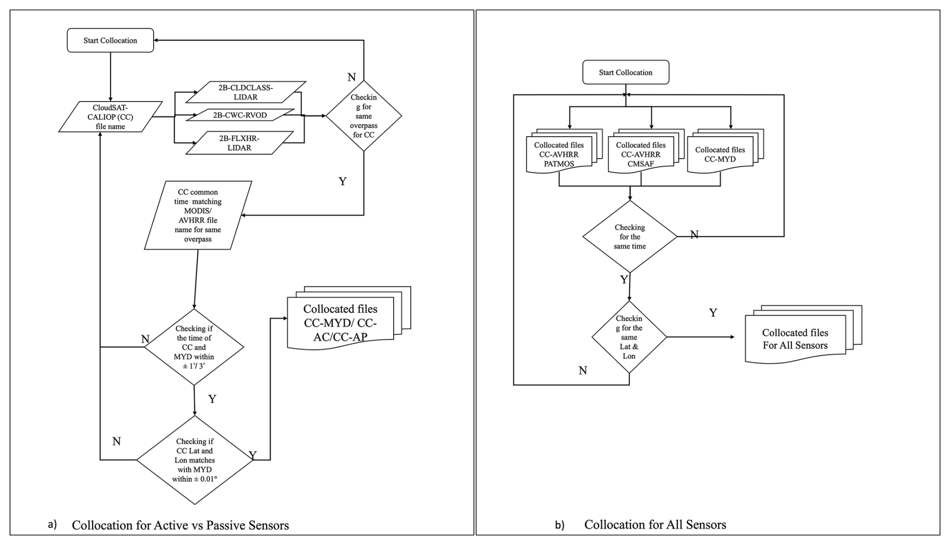
Figure 1 The flowchart of (a) Collocation for MODIS/AVHRR Level 2 data and CloudSat-CALIOP (b) Collocation for all sensors.

An additional limitation of the collocation approach is that true nadir overpasses between passive imagers and CALIOP cannot be achieved over the SO due to orbital geometry. Consequently, many scenes are viewed at oblique angles, which can introduce uncertainties in retrieved cloud top height, optical depth, and cloud fraction relative to nadir CALIOP observations. While this effect is inherent to all three passive satellite data sets, it represents a source of uncertainty that should be considered when interpreting the results, as imagers viewing clouds at oblique angles can impact cloud height, fraction, and optical depth retrievals, when compared to nadir observations of the same clouds.

In order to understand the multilayer cloud influence, a simple empirical multilayer detection (Ritman et al., 2022) mask developed from 2BCL using the difference between two layers and cloud classification was applied to the collocated data. The multilayer cloud mask condition uses the coarsest altitude resolution of 0.3 km, with a minimum gap to define layers of 0.1 km. The cloud layer in the L2 data was first analysed for cloud conditions and classified accordingly as no clouds, quality issues, or cloud layers. The number of cloud layers was assessed using the mask condition and classified as multilayer (hereby abbreviated as ML, referring exclusively to multilayer clouds) or single-layer (SL) clouds. After applying the multilayer detection mask to the collocated pixels, cloud properties were analysed for the multilayer and single-layer conditions.

The cloud properties from the collocated three passive sensors (MYD, AC, AP) and the active sensor (CloudSat-CALIOP) were examined and evaluated against each other. Vertical profiles of case studies with retrieved cloud properties (CTH, COD, CER, and CPH) were also investigated to understand the sensor retrievals. While analysing the case study data, it was found that AP data intermittently substitutes observations from the preceding day in case of missing orbits towards the end of the day. Hence, all case studies within the first two hours and last two hours of each UTC day (00:00–02:00 and 22:00–24:00 UTC) were discarded from the whole year's analyses. The passive sensor CTH and CFC were validated statistically with the active sensor using all the data from 2015. Furthermore, the cloud properties retrieval of COD and CER were compared as a function of the thermodynamic phase (CPH) and multilayer flag. A sea ice flag obtained from AVHRR PATMOS-x data, was used to further understand the potential effects of sea ice on the retrievals.

The evaluation of cloud mask performance skill scores for active and passive sensors was conducted using the Kuiper skill score (KSS; Hanssen and Kuipers, 1965). True positive rates (TPR) and False positive rates (FPR) were calculated using the KSS formula as shown in the equation

$$\begin{array}{}\text{(1)}& \text{KSS}=\text{TPR}-\text{FPR}={\displaystyle \frac{t_{\mathrm{p}}}{(t_{\mathrm{p}}+f_{\mathrm{n}})}}-{\displaystyle \frac{f_{\mathrm{p}}}{(f_{\mathrm{p}}+t_{\mathrm{n}})}},\end{array}$$

where t_p is the number of true positives, f_p is the number of false positives, f_n is the number of false negatives, and t_n is the number of true negatives. A KSS of 1 indicates a high skill score and zero indicates no skill.

Each data set has different definitions of cloud mask and cloud mask uncertainty. The cloud mask for AP has categories including clear sky (0), probably clear (1), probably cloudy (2) and cloudy (3). This was converted to clear (0), encompassing clear sky and probably clear, and cloudy (1), combining probably cloudy and cloudy, for comparison with the other satellite cloud masks. Similarly, MYD cloud masks were classified as cloudy (0) for uncertain (01) and cloudy (00) categories and as clear (1) for confidently clear (11) and probably clear (10). AC has only two classifications: clear (0) or cloudy (1).

We analysed approximately 1.2 million pixels L2 for each sensor. Upon applying the multilayer mask, we observed that approximately 25 % (300 000) of the collocated data consisted of multilayer scenes across the SO. Figure 2 shows the collocated swaths used in the analysis.

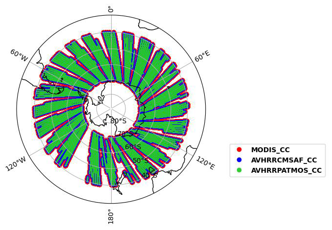
Figure 2 The distribution of collocated Pixels for all 4 sensors. The collocation of MODIS and CloudSat-CALIOP (MODIS_CC) is shown in red, AVHRR CMSAF and CloudSat-CALIOP (AVHRRCMSAF_CC) is shown in blue and AVHRR PATMOS-x and CloudSat-CALIOP (AVHRRPATMOS_CC) is shown in green.

The following sections discuss the results for the monthly data and data comparison for the passive and active sensors.

4 Results and Discussion

4.1  L3 monthly seasonal comparison

The L3 monthly data cloud properties for three sensors: AVHRR CMSAF (CLARA A3), MODIS (CLDPROP_D3_MODIS_Aqua); and CALIOP (CAL_LID_L3_GEWEX_Cloud), were compared for 7 years (2009–2016). The dataset details used for comparison are given in Table 1.

4.1.1 Cloud Top Height

Figure 3 shows the difference in CTH for the top most layer between the active and passive sensors, alongside the SST for the full period and by season. When the data is analysed as a function of latitude band in the ocean region from 62–70° S, both passive sensors generally overestimate the CTHs compared with the active sensor CTHs, except during winter (JJA), when only MODIS overestimates the CTH. This region is typically covered by sea ice during this time of year. The SST also shows variation during corresponding season with a low SST in winter and a high SST in summer. However, there does not seem to be a strong correlation with the differences. In the poles over the land area irrespective of the seasons, AVHRR CMSAF tends to underestimate the CTHs, while MODIS tends to overestimate the CTH. As per Noel et al. (2018), the cloud amount detected by the active sensors and passive sensors varies overall when comparing L3 monthly data. As CALIOP is an active sensor, it is more sensitive to high-thin clouds (CTH>8 km) and the vertical distribution of the clouds. The presence of atmospheric temperature inversions may cause the passive sensor to either underestimate or overestimate the CTHs in the boundary layer (Marchand and Ackerman, 2010). Thus, factors, such as the presence of multilayer clouds, differences in sensor sensitivity and resolution, and differences in retrieval algorithms may account for some of the poor agreement.

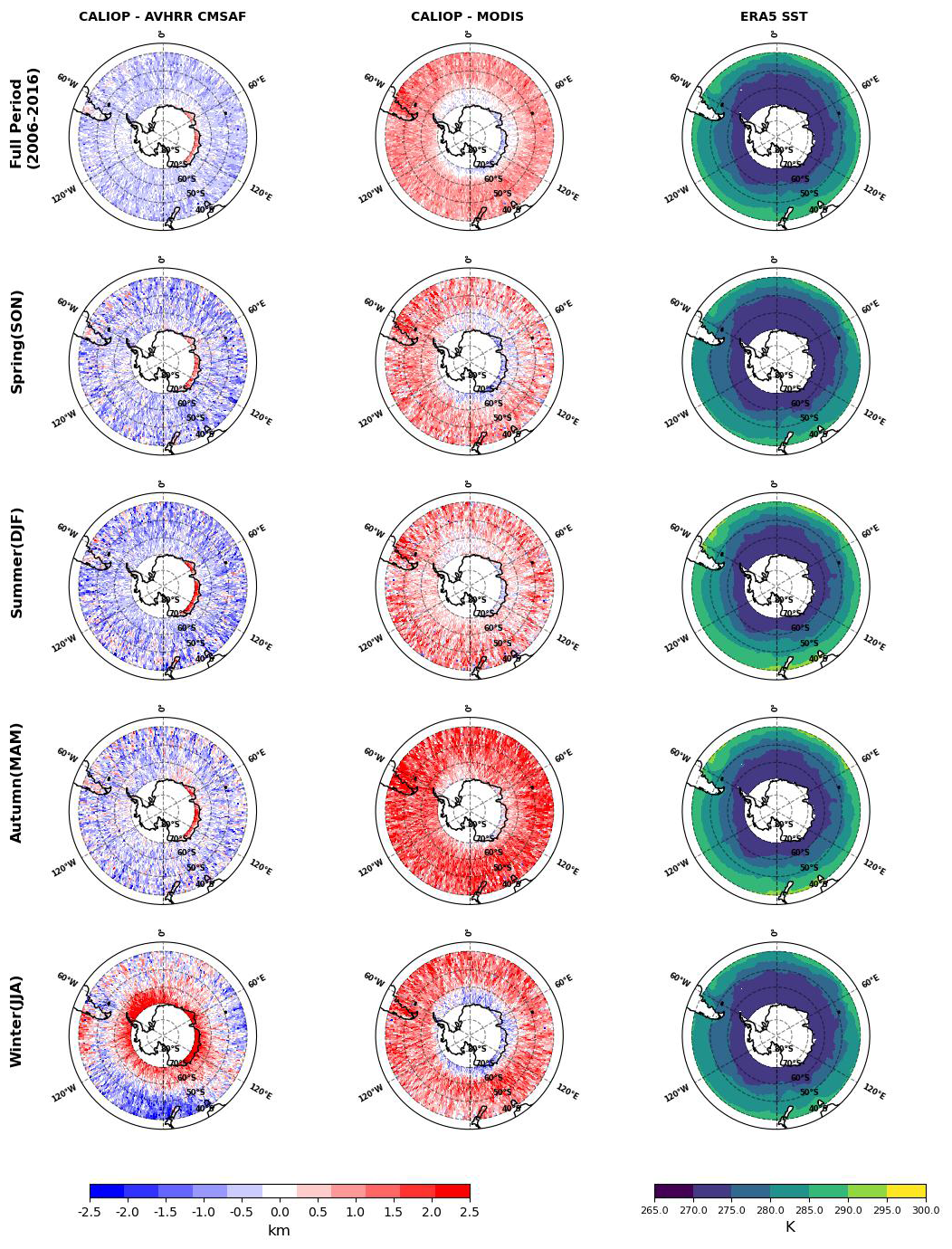
Figure 3 7 year (2009–2016) seasonal data comparison of Cloud Top Heights (CTH), over the Southern Ocean, for Level 3 data retrieved from AVHRR CMSAF (CLARA A3), MODIS AQUA (CLDPROP_D3_MODIS_Aqua) and CALIOP (CAL_LID_L3_GEWEX_Cloud). The left vertical panel shows the difference in CTHs for CALIOP and AVHRR CMSAF , the middle panel CALIOP and MODIS and the rightmost panel shows the SST from ERA-5 data for the same region.

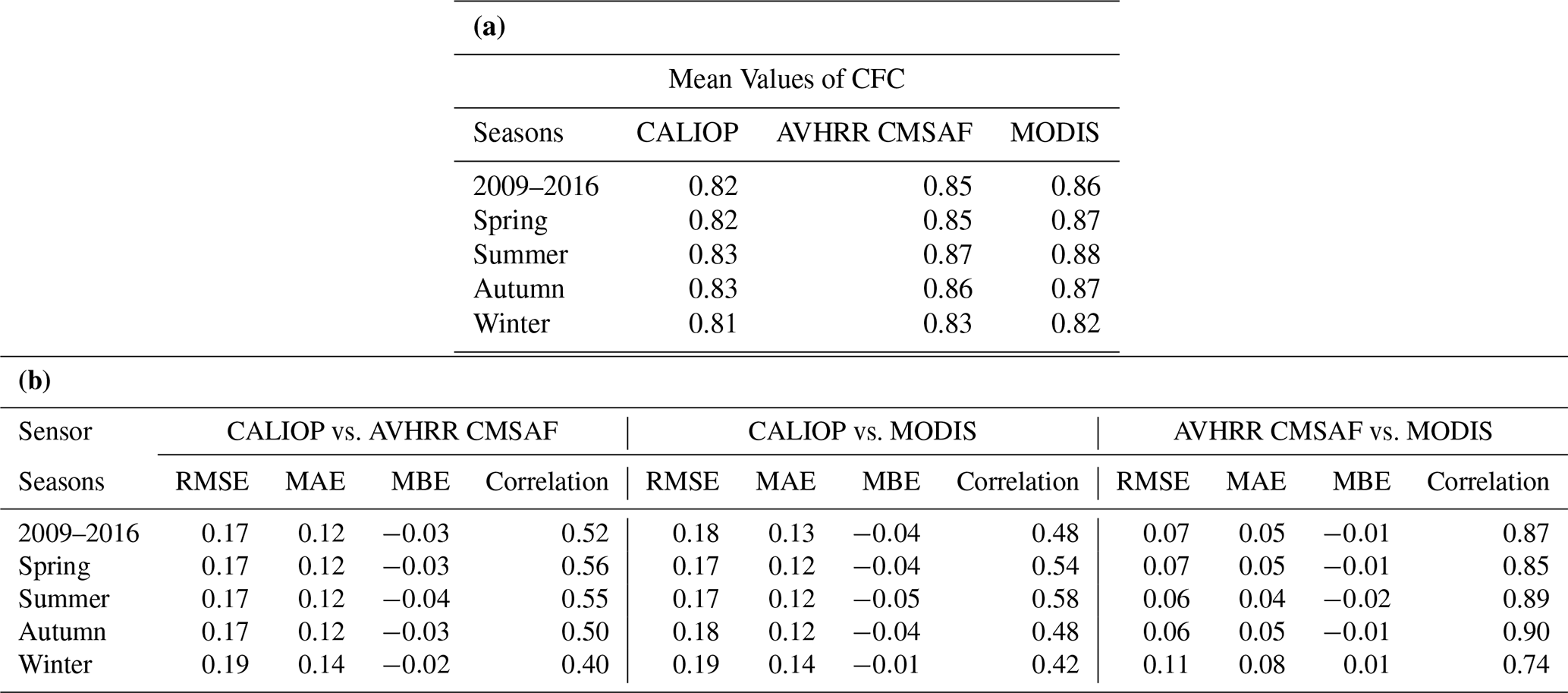
Table 2 summarises the comparisons, with mean CTH values in Table 2a and the statistics for the comparison with CALIOP in Table 2b by season and overall. It can be observed that the active sensor correlation with the passive sensors for the overall monthly CTHs is low with values ranging from 0.36 for CALIOP-AVHRR CMSAF (C-A) to 0.32 for CALIOP-MODIS (C-M). The CTH difference between the C-A sensors for DJF ranges from −1 to 1 km for the study domain, while for C-M it ranges from 0–4 km. The MBE is 0.46 km for C-A and 1.12 km for C-M, showing a larger offset for MODIS. The RMSE for C-A is 2.35 km; for C-M, the value is 2.60 km; and for A-M, it is 0.98 km, which is consistent with both correlation and MBE trend. Overall, the MBE between the MODIS-AVHRR CMSAF (A-M) passive sensors is larger for the CLARA-A3 dataset (0.98 km), but the correlation is 0.68. Overall, there is a positive mean bias error for the passive sensors AVHRR CMSAF and MODIS CTHs.

Table 2 (a) Mean values of Cloud Top Height (CTH) over the Southern Ocean and (b) Statistics for 7 years (2009–2016) monthly data comparison of CTH for Level 3 data retrieved from AVHRR CMSAF (CLARA A3), MODIS AQUA (CLDPROP_D3_MODIS_Aqua) and CALIOP (CAL_LID_L3_GEWEX_Cloud).

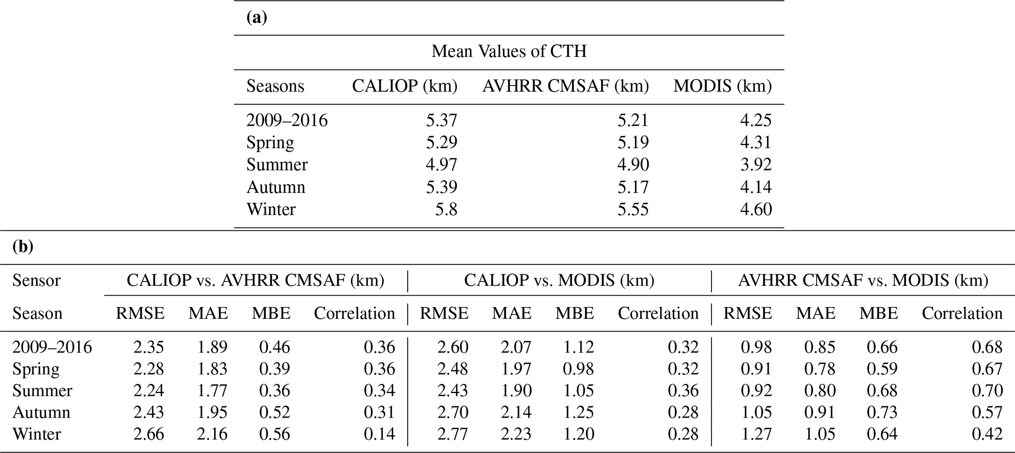
The seasonal comparison of the C-M data over the course of a year shows that the austral autumn (SON) has the weakest correlation (0.28) and MBE (1.25 km). Meanwhile, the inverse is true for the austral summer (DJF) with a correlation of 0.36 and MBE of 1.05 km with MBE>1 km, positive bias over the mid-latitudes, and smaller bias (MBE±0.5 km) over the high-latitudes. Another intriguing observation is that in austral winter (JJA), MODIS overestimates the CTHs in the high-latitude (MBE>1 km) and underestimates in the mid-latitudes(MBE>1.5 km), with an overall season MBE of 1.20 km. The seasonal comparison of CTHs for C-A shows that the correlation is highest in the austral spring (SON) for C-A (0.34) and lowest in the summer (DJF −0.15). AVHRR CMSAF tends to overestimate the CTHs in the mid-latitudes and underestimate them in the high-latitudes during winter, with an overall MBE of 0.25 km. In all other seasons, AVHRR CMSAF tends to overestimate the CTHs across the region, with the exception of Antarctica.

The passive sensor comparison shows that DJF has the highest correlation at 0.68, whereas JJA has the lowest at 0.45. Additionally, DJF exhibits the lowest mean bias error of 0.09 km for C-A among all seasons and 0.98 km for C-M. This may be due to the seasonality of cloud cover over the SO, as JJA tends to have more high-clouds (Bromwich et al., 2012) and passive sensors fail to detect the cloud due to poor sensor sensitivity to optically thin high clouds. The results indicate that the AVHRR CMSAF generally shows a tendency to overestimate the CTHs compared to CALIOP, although in some subregions (e.g. Antarctic land) it underestimates. Conversely, MODIS tends to underestimate the CTHs overall, but can overestimate in specific latitude bands such as 62–70° S.

4.1.2 Cloud Fraction

The comparison of CFC for the active and passive sensor data overall and seasonally is shown in Fig. 4. The overall 7 year mean CFC values for the SO were 0.82 for CALIOP, 0.86 for MODIS, and 0.85 for AVHRR CMSAF. This is consistent with the findings of the review study conducted by Bromwich et al. (2012). The cloud fraction for all sensors, both passive and active, has more cloud cover over the mid-latitudes (40–60° S) than over the high-latitudes (>60° S). In general, the cloud cover decreases (<70 %) towards very high-latitudes near the coast of Antarctica for all sensors, which is also consistent with findings of Bromwich et al. (2012). This decrease, especially in winter, is likely due to the presence of sea ice near the Antarctic coast. This inhibits the flux of water vapour (surface evaporation), as presented in studies by Frey et al. (2018) and Wall et al. (2017). The high cloudiness for this area can be attributed to the frequent synoptic-scale and mesoscale depressions and intense cyclonic activity around the Antarctic Continent (Carrasco et al., 2003; King and Turner, 1997; Simmonds et al., 2003). In general, the passive sensors have higher cloud coverage than CALIOP observations for the higher latitude.

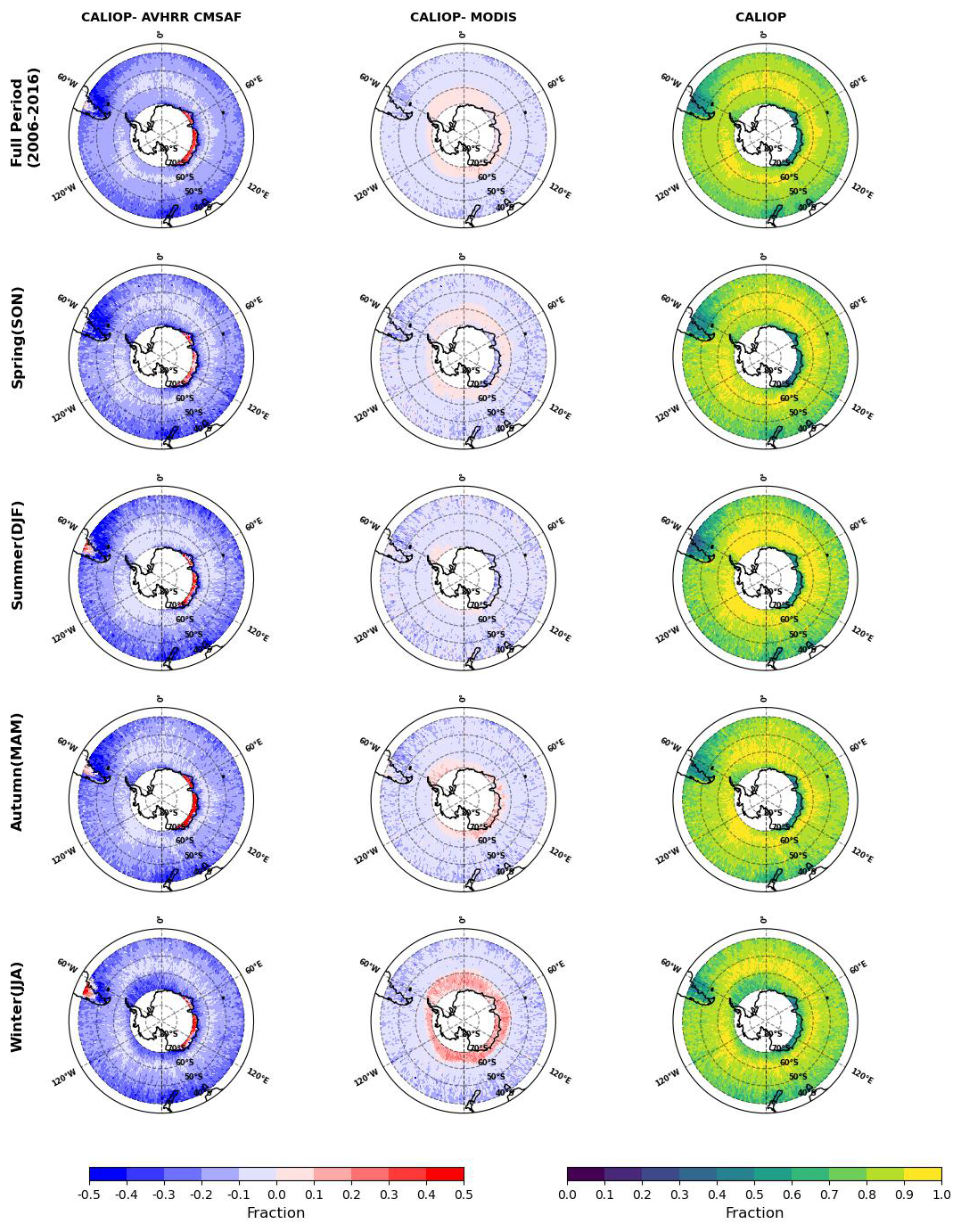
Figure 4 7 year (2009–2016) seasonal data comparison of Cloud Fraction (CFC), over the Southern Ocean, for Level 3 data retrieved from AVHRR CMSAF (CLARA A3), MODIS AQUA (CLDPROP_D3_MODIS_Aqua) and CALIOP (CAL_LID_L3_GEWEX_Cloud). The left vertical panel shows the difference in CFCs for CALIOP and AVHRR CMSAF, the middle panel CALIOP and MODIS and the rightmost panel CALIOP CFC for the same region.

The detailed mean and statistics for the CFC comparison are given in Table 3. It's intriguing to note that the correlation between the passive sensors (AVHRR CMSAF and MODIS) and the active sensor (CALIOP) is low (0.52 and 0.48) over the whole period. On the other hand, the correlation between the passive sensors is higher (0.87), which suggests that the L3 passive retrievals may have a different systematic bias. Bromwich et al. (2012) also observed a difference in the cloud cover for the passive and active sensors, they attributed this to the spatial resolution issues of the active sensor when compared to the passive sensor. The results of this analysis indicate that the active sensor cloud cover was less than the passive sensors, by approximately 4 % for MODIS and AVHRR CMSAF. Note that we are comparing against the CALIOP passive sensor adjusted data set.

Table 3 (a) Mean value of Cloud Fraction (CFC) over the Southern Ocean and (b) Statistics for 7 years (2009–2016) monthly data comparison of CFC for Level 3 data retrieved from AVHRR CMSAF (CLARA A3), MODIS AQUA (CLDPROP_D3_MODIS_Aqua) and CALIOP (CAL_LID_L3_GEWEX_Cloud).

We found that CFC values are slightly lower in JJA (winter), with a mean of 0.83 and 0.82, respectively, compared to DJF (summer) when we compared AVHRR CMSAF and MODIS L3 data. In the case of MODIS, the high latitude CFC for JJA is approximately 60 %, the lowest amongst all the sensors. This can be attributed to the presence of sea ice. For the active sensor, JJA has the lowest CFC (0.81). It's also observed that there is a notable difference in cloud cover over land for different passive sensors. MODIS overestimates the cloud cover over land; on the other hand, AVHRR CMSAF underestimates the cloud cover compared to the active sensors. In the RMSE and MAE seasonal analysis for all sensor comparisons, it was found that JJA has the highest value for both amongst all seasons. However, for the MBE, it's the opposite, with JJA having the lowest value (≈0.01 km) for all sensors. The correlation also follows the same trend as MBE errors: low in JJA and high in DJF. For comparisons among the passive sensors, the agreement of pixels identified as cloudy by both sensors is more consistent, and the root mean square error (RMSE) is low for all seasons. All of the comparison's seasonal findings are consistent with the conclusions of Bromwich et al. (2012).

The results indicate that CALIOP detects fewer clouds than the passive sensors. This could be due to a difference in resolution or in the approach taken to make the L3 data set comparable with passive sensors. The total cloud cover for the SO was found to be around 86 % (MODIS), 85 % (AVHRR CMSAF) for passive sensors and 82 % for CALIOP.

4.1.3 Cloud fraction for liquid clouds

The overall cloud fraction of liquid water clouds (hereafter CFL) and seasonal distributions are illustrated in Fig. 5. For the entire year, CALIOP, AVHRR CMSAF, and MODIS show the presence of liquid clouds at around 50 %. In terms of the correlation for the CFLs, the passive sensor comparison is better (0.71) than the active sensor comparison (0.37 C-A and 0.44 C-M). Lachlan-Cope (2010) observed that over Antarctica, ice clouds are more prevalent and along the coast of Antarctica, mixed-phase clouds are more prevalent. Other studies also observed that mixed-phase clouds are prevalent over the SO (Ahn et al., 2017; Huang et al., 2012; Mace et al., 2021) as they are usually misclassified more over the SO. From Fig. 5, we can conclude that AVHRR CMSAF is identifying more liquid clouds over the high-latitudes than other products, while other passive products classify the clouds as ice clouds or mixed-phase clouds. The comparison's mean and statistical analysis are given in Table 4. The comparison shows that AVHRR CMSAF primarily overestimates the CFL, while MODIS tends to underestimate it when compared to CALIOP. However, around the high-latitudes, towards the coast of Antarctica the AVHRR CMSAF underestimates the CFL when compare to CALIOP. In the case of seasonal comparisons, the correlations for passive sensors against active sensors are low overall in all seasons. For all the sensors, the CFL is consistently higher in DJF and the lowest in JJA. When we look at the MBE, AVHRR CMSAF has a negative bias for all seasons, while MODIS has a positive bias for all seasons compared to CALIOP. AVHRR CMSAF exhibits the smallest bias in JJA and the highest in DJF, while MODIS displays the smallest bias in DJF and the highest in JJA. This suggests a discrepancy in cloud classification during the liquid phase between the sensors in DJF. This disagreement can be attributed to the presence of supercooled liquid in DJF (Huang et al., 2015; Bodas-Salcedo et al., 2016). The C-A seasonal comparison reveals that the AVHRR CMSAF overestimates the liquid cloud cover across the study region in DJF and JJA, with the exception of Antarctica, where it underestimates the amount of liquid cloud. However, in SON and MAM towards the latitudes>55° S, both sensors underestimate the CFL. The presence of sea ice explains this difference in SON and MAM. In summary, the comparison of the L3 data for the CTH shows a bias in the retrieval between passive sensors, underestimating the CTH by around 1 km compared to the active sensor: the mean bias error was 0.96 km (C-A) and 1.12 km (C-M). The study of L3 CFC and CFL revealed that AC overestimates the amount of clouds compared to observations made by MODIS and CALIOP, with the overestimation increasing during the winter months.

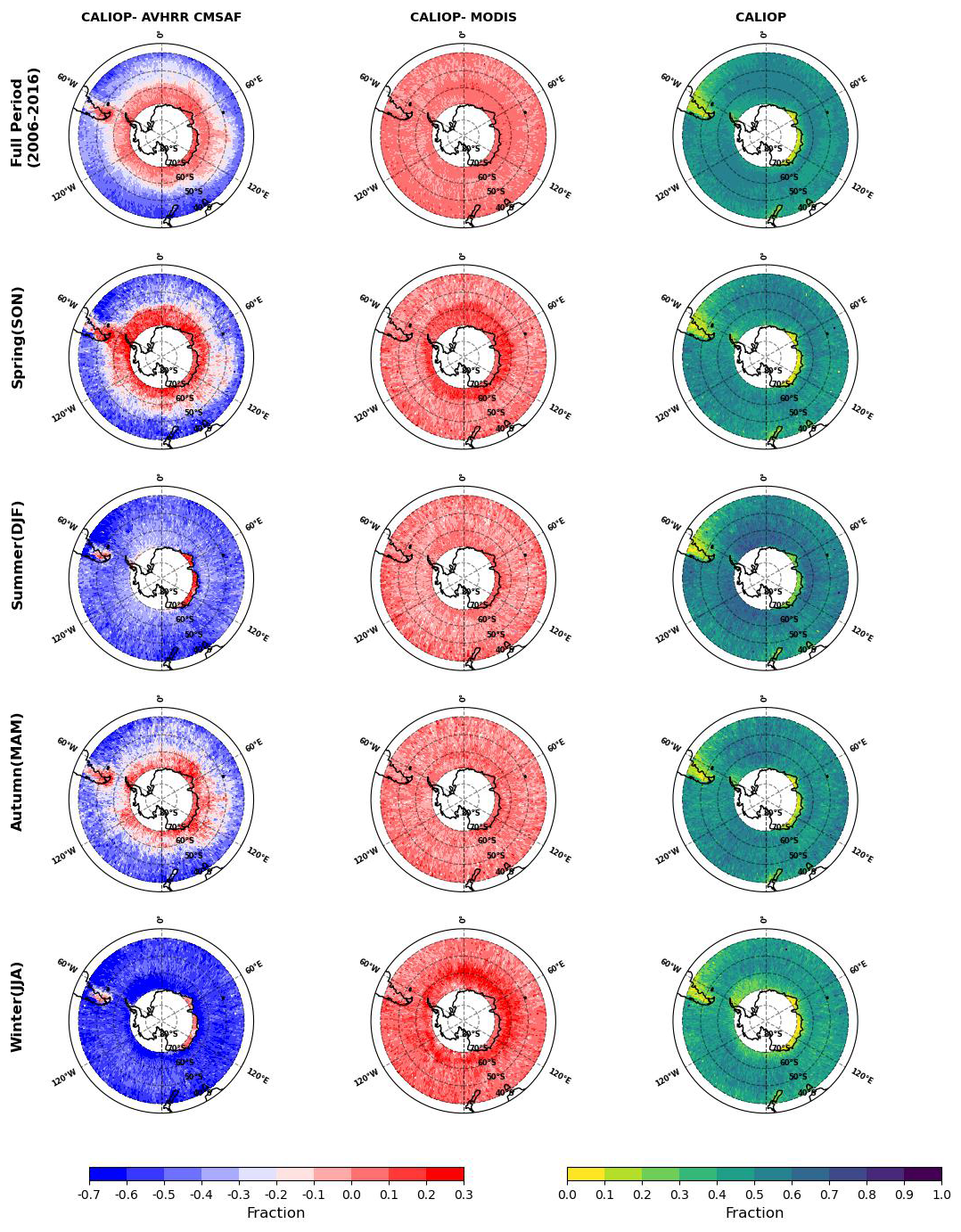
Figure 5 7 year (2009–2016) seasonal data comparison of Liquid Phase Clouds Fraction (CFL), over the Southern Ocean, for Level 3 data retrieved from AVHRR CMSAF (CLARA A3), MODIS AQUA (CLDPROP_D3_MODIS_Aqua) and CALIOP (CAL_LID_L3_GEWEX_Cloud). The left vertical panel shows the difference in CFLs for CALIOP and AVHRR CMSAF, the middle panel CALIOP and MODIS and the rightmost panel shows CALIOP CFL for the same region.

Table 4 (a) Mean Liquid Phase Clouds Fraction (CFL) values over the Southern Ocean and (b) Statistics for 7 years (2009–2016) monthly data comparison of CFL for Level 3 data retrieved from AVHRR CMSAF (CLARA A3), MODIS AQUA (CLDPROP_D3_MODIS_Aqua) and CALIOP (CAL_LID_L3_GEWEX_Cloud).

4.2  Results for Level 2 pixel-wise comparison

4.2.1 Case study on the 19 October 2015 at 08:37 UTC

To illustrate these differences in retrieval behaviour, we present a case study over the SO on 19 October 2015, which was used to examine how passive and active sensors capture cloud properties under varying cloud structures. Figure 6 shows the 11 µm brightness temperature swaths for MODIS and CTH swath for MODIS (MYD), AVHRR PATMOS-x (AP) and AVHRR CMSAF (AC) and in black the merged CloudSat-CALIOP track for the 19 October 2015 at 08:37 UTC. Although all three sensors observed a similar high cloud pattern around 50° S: AC retrieves the CTH at around 11 km height, while MYD and AP retrieve the CTH at around 9 km height. Finally, AP has a significant region of cloud with CTHs at around 5 km height located at 40° S and 80° E, while AC and MYD observed low clouds with CTHs at around 2 km height for the same region.

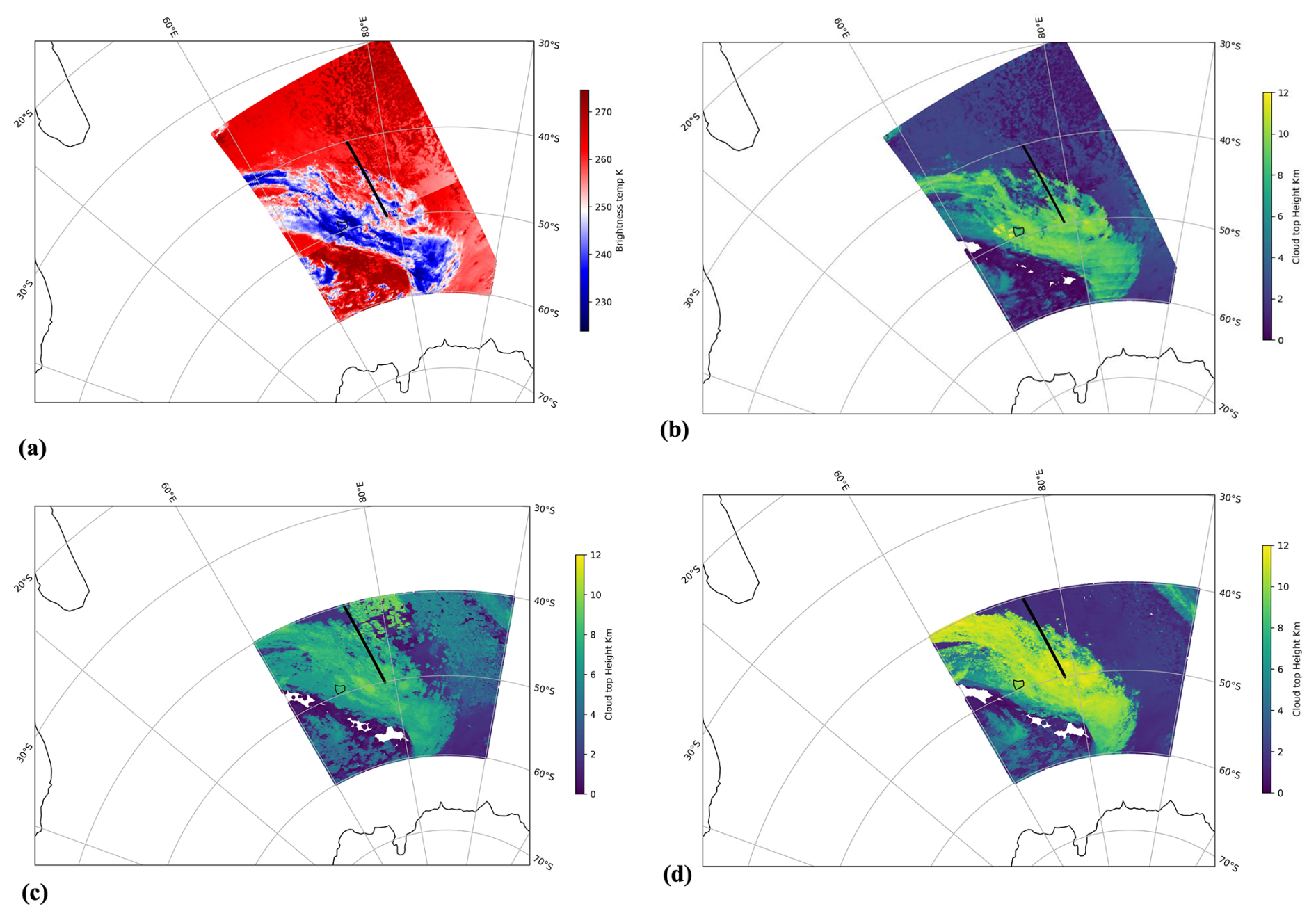
Figure 6 Swath for (a) brightness temperature retrieved from MODIS (MYD), (b) Cloud top height retrieved from MODIS (MYD), (c) AVHRR PATMOS-x and (d) AVHRR CMSAF with swath plot of merged CloudSat-CALIOP (CC), shown in black, for Case study on 19 October 2015 at 08:37 UTC.

Figure 7 shows a curtain plot for the CC track and the corresponding CTH, COD, CER, and CPH for each instrument. The top panel shows the CTH for all passive sensors (AC, AP, MYD, and CC), as well as the vertical profile of COD from the CC dataset (2BFL). The CTH for CC at a COD limit of 0.5 is also shown (cyan) to illustrate the potential differences in optical depth sensitivity between the passive and active sensors. The second panel illustrates the COD for the four sensors, along with the multilayer mask derived from CC. The COD was derived using the 3.7 µm channel, as it is common to all passive sensors. The third panel displays the CER, as well as the sea ice mask used in the AP retrieval. The bottom panel shows the cloud phase for each instrument; for CC the phase is the phase detected at the top of the cloud. This example illustrates the highly variable nature of the cloud field across the Southern Ocean. Our discussion focuses on three sub-sections: multilayer clouds (Fig. 7a[i]); thick upper-level clouds over thick lower-level clouds (Fig. 7a[ii]); and optically thick boundary layer clouds (Fig. 7a[iii]).

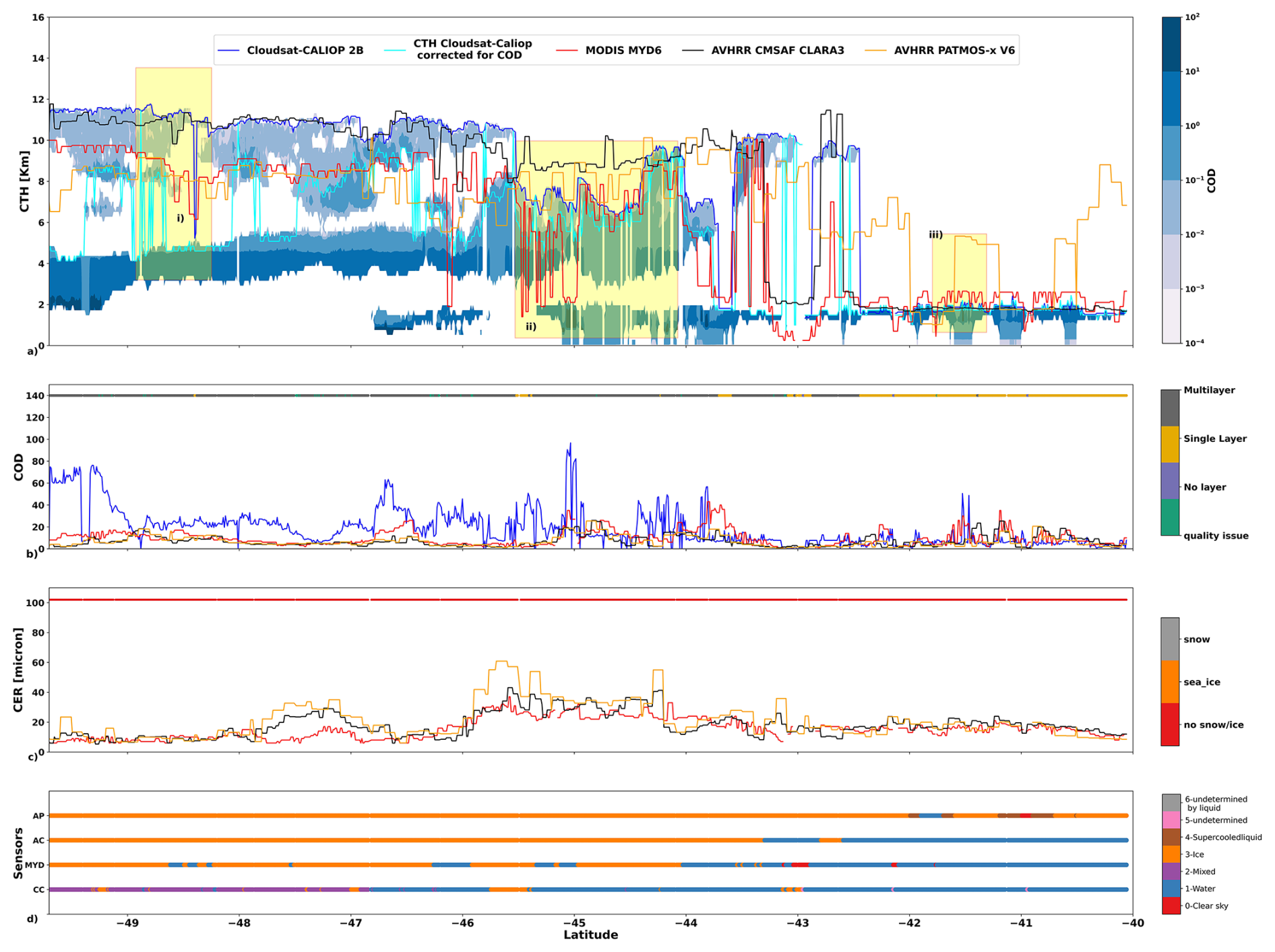
Figure 7 Vertical profiles for cloud properties Cloud Top Height (CTH; Top panel), Cloud Optical Depth (COD; Second Panel), Cloud Effective Radius (CER; third panel) and Cloud Phase (CPH; Bottom Panel) retrieved from collocated data of AVHRR CMSAF (AC), AVHRR PATMOS-x (AP), MODIS (MYD) and merged CloudSat-CALIOP (CC) for Case study on 19 October 2015 at 08:37 UTC.

In the first panel, the CTH ranges from 0–12 km height and shows substantial differences between the CTH of passive and active sensors, with both underestimation and overestimation by passive sensors compared to CC. Figure 7a[i] shows a multilayer cloud structure with an optically thin high-level cloud over optically thick mid-level clouds. MODIS and AP detect the high-level cloud, however since it is optically thin over an optically thick lower layer cloud, it places the CTH at an effective CTH between the upper and lower layers. For the AC retrieval, the CTH is similar to the CC height. In Fig. 7a[ii], AC produces higher CTH values than CC, MYD yields lower values, and AP's results are closest to those of CC. This difference could be due to the different numerical weather prediction (NWP) reanalyses used temperature profiles. Indeed, the CTH can vary substantially, particularly at high altitude and depends on the difficulty in identifying the inversion at the tropopause (Wu et al., 2012; Müller et al., 2018).

Figure 7a[iii] shows a region of boundary layer clouds around 41.5° S. AC does a good job of retrieving the boundary layer cloud, while AP boundary layer CTH can show large over estimations, and MYD occasionally over and underestimates. Boundary layer clouds can be difficult to estimate, particularly when temperature inversions are present, as they can present multiple solutions when using the thermal characteristics to retrieve CTH (Huang et al., 2012; Wall et al., 2017; Truong et al., 2020). AP misclassifies the phase between 41.5–40° S which may explain the high CTH retrieval and highlights some internal dependency in the retrieval approach.

The second panel (Fig. 7b) displays the CC multilayer mask and identifies the areas with multilayer clouds well. The COD for each retrieval is also compared in the second panel. The COD of CC (2BFL) exhibits high variability when compared to the COD of the passive sensors, particularly for ML clouds. CC COD is substantially higher than that of the other sensors. The COD has large differences among the passive sensors and active sensor in the presence of a multilayer structure (Fig. 7a[i] and [ii]); In single-layer areas, the COD of MYD, AP and AC are more in agreement with the active sensor measurements. The results align with the product statement for CC COD (Henderson and L'Ecuyer, 2023) which states that the COD is similar to MYD for single layer and varies with multilayer clouds. The third panel (Fig. 7c) shows the CER comparison and the sea ice flag. While the general pattern of the CER from the passive sensors is in agreement, the values of AP CER are higher than MYD and AC CER retrievals in general, particularly where ice clouds detected are quite different.

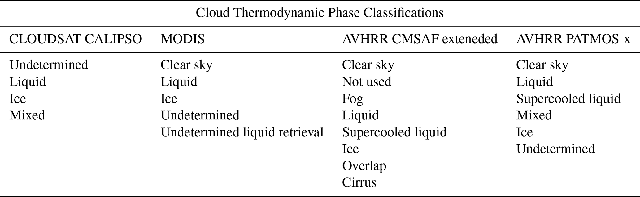
The cloud phase is shown in the fourth panel (Fig. 7d). For CPH, each retrieval algorithm uses a slightly different phase classification scheme. The CC retrievals classify the phase as mixed, liquid or ice phase on the basis of cloud top and base temperatures, radar reflectivity and integrated attenuated backscattering coefficient across all the cloud layers in the vertical column (Wang, 2019). For the passive sensors (MYD, AP and AC), the CPH is the phase detected at the top of the cloud. In the case study, all sensors share ice and liquid as common classes, with an additional clear sky class for MYD, a supercooled liquid class for AP, and a mixed phase class for CC. Further classification of the phase can be seen in Table 5. The agreement between the passive sensors overall is good with occasional differences; for example, at 43° S, AC and MYD classify the cloud phase as liquid while CC and AP classify it as ice, with cloud optical depth indicating a thin upper layer.

Table 5 Cloud Thermodynamic Phase classification for Level 2 AVHRR CMSAF (AC), AVHRR PATMOS-x (AP), MODIS (MYD) and CloudSat-CALIOP (CC)..

To summarise, we observe significant variations in the retrieved cloud properties in the presence of multilayer clouds, with passive sensors both overestimating and underestimating the retrieved CTH compared to active sensors. The dependency on the optical depth on the topmost cloud layer, the penetrative property, and the sensitivity of passive sensors are seen in this case study. The case study demonstrates that cloud property retrievals differ based on cloud type, retrieval algorithm, and sensor sensitivity. Multilayer clouds often exhibit the greatest discrepancies.

4.2.2 L2 cloud mask

The cloud mask products from the passive sensors are evaluated against the CloudSat-CALIPSO product (Table 6). The true positive rate (TPR) is similar for AVHRR CMSAF (0.94) and AVHRR PATMOS-x (0.94) and smaller for MODIS (0.77). The false positive rate (FPR) vary considerably among the products, 0.22 for AC, 0.07 for MYD, and 0.51 for AP. The Kuiper Skill scores are relatively similar, 0.71 for AC, 0.70 for MYD, except for AP, 0.43. The higher resolution of MODIS may contribute to the higher KSS compared to AVHRR PATMOS-x.

Table 6 Cloud mask performance for 2015 over the Southern Ocean comparison for Level 2 AVHRR CMSAF, AVHRR PATMOS-x and MODIS against active sensor CloudSat-CALIOP (CC).

According to Karlsson et al. (2023a), when the global cloud masks of the CLARA A3 and CALIPSO (5 km cloud product) were compared, for the years 2006–2015, the overall hit rate was 0.82 and the KSS score was 0.68. The hit rate for high latitudes in both hemispheres was 0.85, and the KSS score was 0.69. For polar regions, the hit rate was 0.69, and the KSS score was 0.49. The KSS score from our analysis comparing AC cloud mask and CC is 0.71, is similar, but the hit rate is higher (0.94). The differences could be attributed to the active sensor data considered (CC and CALIPSO) i.e. differences in CC cloud masking algorithms and the validation method. The hit rate for MYD and CC comparison is the lowest (0.77); on the other hand, the FPR is also the lowest amongst the sensors (0.07). In conclusion, the comparison of KSS scores and hit rates across different sensors and regions revealed variations that highlight the importance of balancing FPR and hit rate, passive cloud masking algorithms, and validation methods in evaluating cloud detection accuracy.

4.2.3 L2 cloud top height comparison

Figure 8 shows a 2D histogram plot of passive satellite CTH compared with active (CC) CTH for the year 2015. A summary of the comparison of the average CTH with and without a COD limit>0.5 is given in Table 7. We chose a COD threshold of 0.5 to exclude optically thin clouds that are often detected by CALIOP but missed or poorly retrieved by passive sensors, consistent with previous studies (Karlsson et al., 2017; Marchant et al., 2020; Yost et al., 2023).

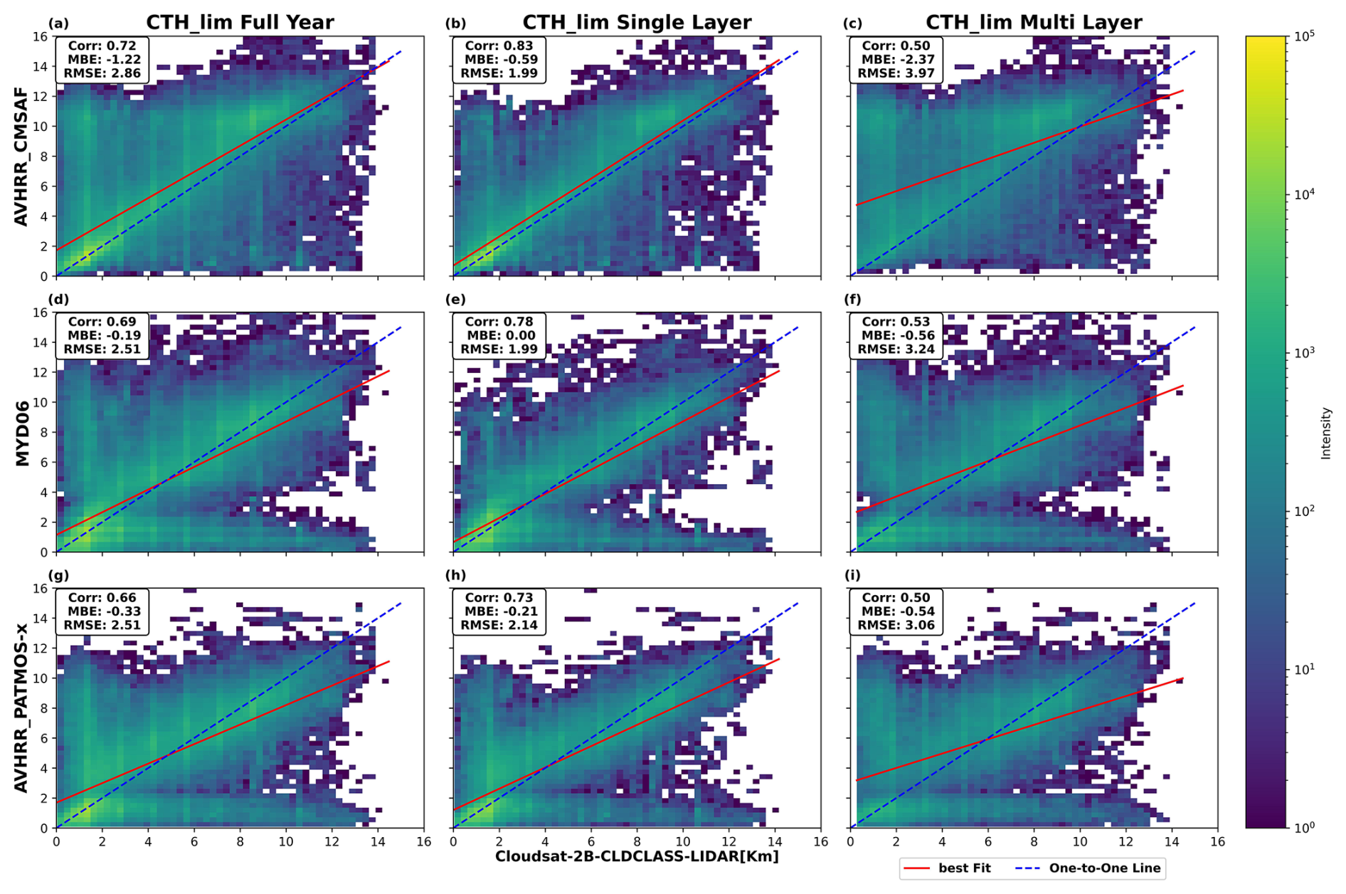
Figure 8 Collocated Level 2 AVHRR CMSAF (top), MODIS (middle), AVHRR PATMOS-x (bottom) and CLOUDSAT-CALIOP merged data analysed for Cloud Top Height (CTH), over the Southern Ocean, for 2015 (left) shows the Joint 2D Histogram for CTHs, the 2D histograms for multilayer (right) and single-layer (centre) masked collocated data.

Table 7 (a) Mean Cloud top height (CTH) values for 2015 over the SO for Level 2 CTHs data MODIS (MYD), CloudSat-CALIOP (CC), AVHRR CMSAF (AC) and AVHRR PATMOS-x (AP). Statistics of the comparison of CC CTH with the COD limit>0.5 is shown in (b, c) is for CC CTH without the COD limit.

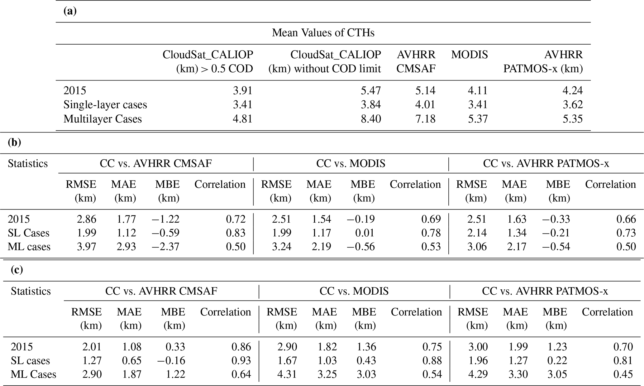
The average CTH of CC is higher without the COD limit, indicating that the high thin cloud is removed when this threshold is applied. In general the average height of passive sensors is higher than the CC with CTH threshold>0.5 and lower than the CTH without threshold. Analysis of the full dataset (2015) reveals mixed agreement between passive and active sensors, with AC (5.37 km) demonstrating better agreement than CC CTH without threshold (5.14 km), and AP (4.24 km) and MYD (4.11 km) demonstrating better agreement with CC CTH with COD>0.5 (3.91 km). For both CC mean CTH (with and without COD>0.5), single-layer clouds (3.41 and 3.84 km), passive sensors exhibit good agreement with each other.

Multilayer cloud identification was applied using a mask derived from CC CTH. The results for the multilayer cloud are unsurprisingly less accurate and inconsistent. The AC mean CTH (7.18 km) shows better agreement with the CC mean CTH without the threshold (8.40 km), indicating that it is more sensitive to the mean CTH of high thin clouds than MYD (5.37 km) and AP (5.35 km), which show better agreement with the CC CTH COD>0.5 threshold (4.81 km).

Figure 8 shows a 2D histogram comparison of passive satellite CTH with active (CC) CTH for 2015. The CC CTH plotted was CTH with a COD>0.5. Each row shows the results for a single passive satellite: AC is the top row (Fig. 8a–c), MYD is the second row (Fig. 8d–f) and AP is the bottom row (Fig. 8g–i), each column shows the result, from left to right: the full dataset (2015), single-layer clouds, and multilayer clouds.

A number of features become apparent in Fig. 8 MYD and AP plots display a horizontal band, signifying the passive sensor's underestimation of the CTH, which aligns with the earlier analysis. In general, the CTH of low clouds are overestimated by the passive sensors. The passive sensors underestimate the CTH of high clouds in MYD and AP. An explanation for the overestimation of low CTH is the presence of a sharp temperature inversion that provides two solutions for the same IR temperature from the NWP reanalyse profile, one above and one below the actual CTH (Fig. 7a[iii], Dong et al., 2008). For clouds that have underestimated the CTH, there are two possible reasons for this. Firstly, the clouds are thin and the retrieval does not properly account for the extinction of the cloud or a contribution to the TOA radiance from the surface (Fu et al., 2017). Secondly, the passive sensor IR channels often penetrate into the clouds, as seen clearly in the case study Fig. 7a[ii].

The differing performance of the passive data sets is in part due to different algorithm approaches. The AC CTH has been derived by training a neural network with collocations of CALIOP cloud top heights. While the MYD retrievals uses a physical model based on CO₂ slicing and IR window approach (Menzel et al., 2015) for the retrieval of CTH. In AP, CTHs are retrieved using physical models, the ACHA algorithm and the CO₂ slicing method (Menzel et al., 2008). As the results of the CO₂ slicing method were poor, we have considered only the ACHA method CTHs. The ACHA methods employs a combination of IR channel observations and the split-window approach (Heidinger and Pavolonis, 2009), to retrieve the CTHs.

The analysis of L2 CTH properties has shown significant differences between products. There are differences not only between retrievals using the same instrument (AP and AC), but also between retrieval algorithms and between different instruments. The agreement between all sensors was reasonable for cloud top heights in the case of single-layer scenes. However, scenes classified as multilayer exhibited a lower level of agreement. The general findings on CTH are in agreement with previous studies (Hollmann and Wetterdienst, 2020; Yang et al., 2021). Mitra et al. (2021) observed the maximum CTH uncertainty for MODIS (L2) for a single-layer unbroken low cloud of 0.540±0.690 km. In the MYD collection, CTH bias with CALIOP was reduced to 0.197 km for low-level boundary liquid clouds (Baum et al., 2012).

In our comparison of the overall L2 collocated data of active and passive sensors, the mean bias in each sensor for CTH, against CC without threshold, varies with MODIS (MYD) 1.36 km, AVHRR CMSAF (CLARA A3) 0.33 km and AVHRR PATMOS-x (V6) 1.23 km. When it comes to multilayer classified pixels, the passive sensors mean bias substantially underestimates the CTH (MYD – 3.03 km, AC – 1.22 km, and AP – 3.05 km). Given that the total number of multilayer identified scenes represents one-fourth of the total scene, the bias is considerable. Overall, the AC neural network retrievals performed the best, delivering higher sensitivity to thin clouds and performing significantly better for multilayer and high clouds.

4.2.4 L2 Cloud Effective Radius Comparison

This section compares CER from the passive sensors as a function of CPH and the presence of single or multilayer clouds. The passive sensors categorise thermodynamic phase into various classifications according to their retrieval algorithms and the categories used by each dataset are presented in Table 5. In the results presented, the number of classes was reduced: classifications of water, fog, and supercooled liquid are grouped as liquid; ice, cirrus, and overlap are treated as ice. When this generalised CPH classification is used, more liquid-phase clouds are found in SL cases, while ice dominates in ML cases. A comparison between the different sensors AC, MYD, and AP is illustrated in Fig. 9 for the year 2015, stratified for SL and ML cases, and summarised in Table 8.

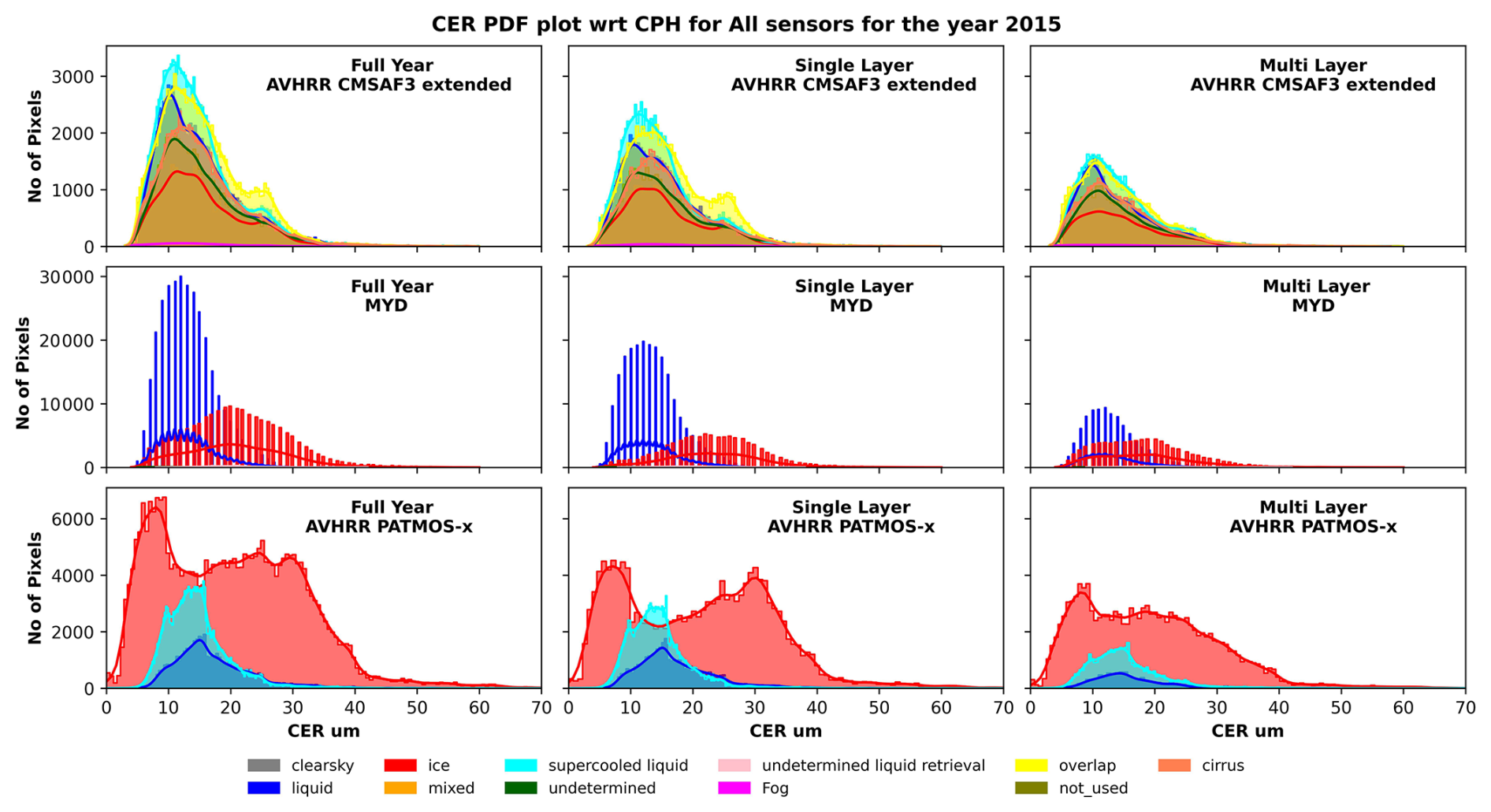
Figure 9 Cloud Effective Radius (CER) distribution according to the cloud phase for the collocated data for the year 2015, over the Southern Ocean, for all passive sensors.

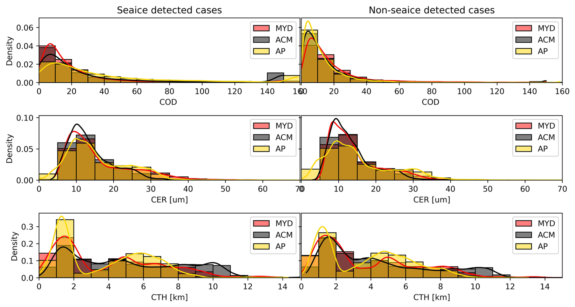
Figure 10 Cloud Optical Depth (COD), Cloud Effective Radius (CER) and Cloud Top Height (CTH) as a function of Sea ice Flag from AVHRR PATMOS-x for all passive sensors, over the Southern Ocean. MODIS (MYD) is shown in red, AVHRR CMSAF (AC) is shown in black and AVHRR PATMOS-x (AP) is shown in yellow.

Table 8 Mean and Median Cloud Effective Radius (CER) comparison for 2015 over the Southern Ocean, for liquid, ice and supercooled liquid phases from Level 2 AVHRR CMSAF (AC), AVHRR PATMOS-x (AP), MODIS (MYD) and CloudSat-CALIOP (CC).

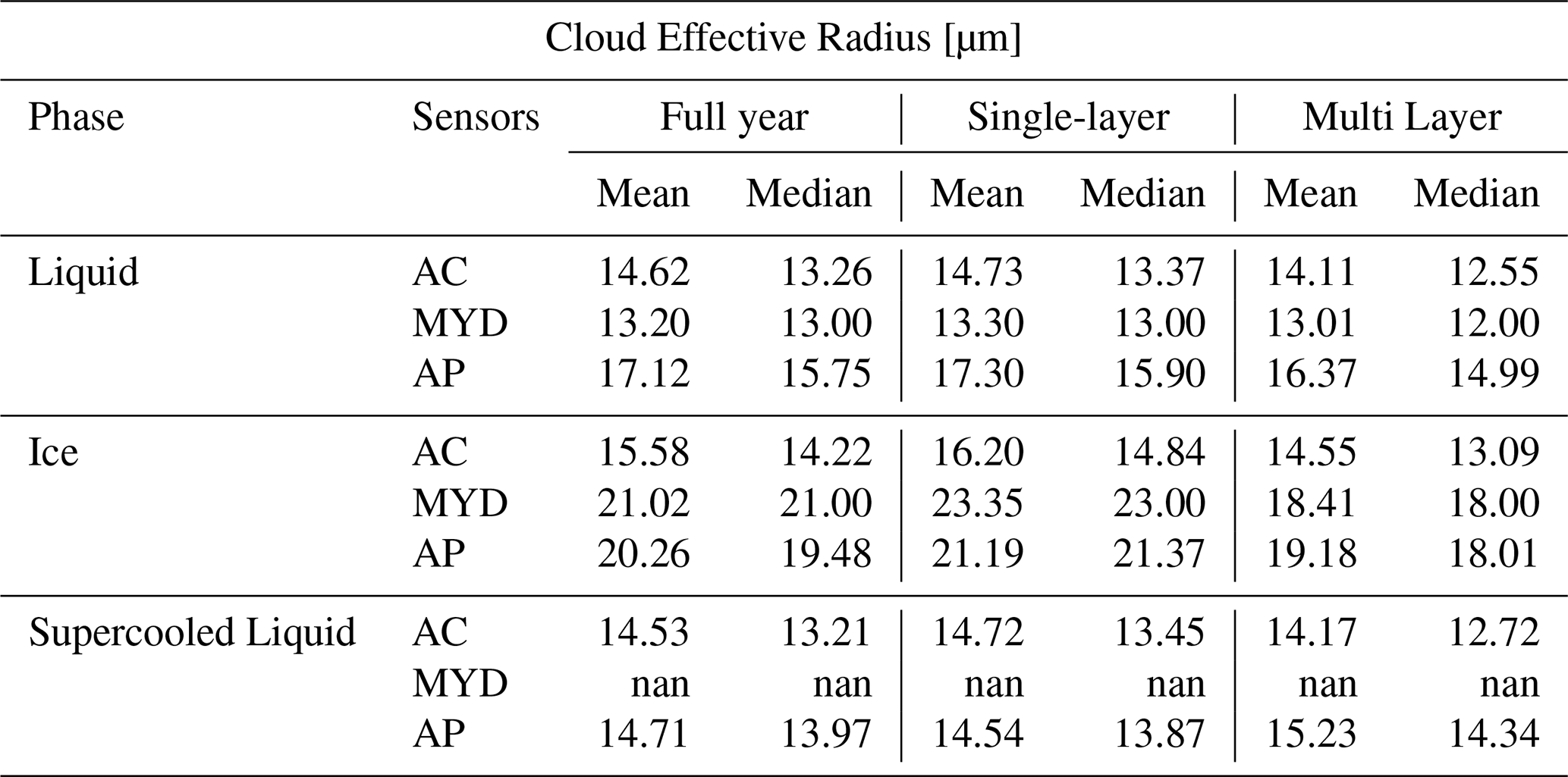
The liquid CER probability density functions (PDFs) are in broad agreement across the three sensors for all cases. The mean values for liquid clouds are approximately 14 µm for AC, 13 µm for MYD, and 17 µm for AP. The higher CER values from AP suggest potential misclassification of liquid clouds as ice clouds as the proportion of ice clouds in AP is over five times higher than that of liquid clouds. The liquid phase occurs more frequently in SL clouds than ML clouds across all sensors, with similar mean values for both cases (Table 8).

In contrast, the CER comparisons for ice-phase clouds reveal notable differences across the sensors. The overall mean for AC is 15.58 µm, while MYD and AP report means of 21.02 and 20.26 µm, respectively. AP also exhibits a distinct bimodal CER distribution with peaks at approximately 10 and 30 µm, particularly evident in SL ice-phase retrievals. ML cases show more similar CER distributions across the sensors. The SL–ML CER difference is relatively small for AC (≈1 µm), modest for AP (≈2 µm), and larger for MYD (≈5 µm). Sensitivity to ice crystal habit selection and the corresponding LUT structure also influences retrievals. MYD uses scattering functions derived from the General Habit Mixture (GHM) developed by Baum et al. (2005a, b) and Yang et al. (2013), implemented as band-specific LUTs (Platnick et al., 2016; Amarasinghe et al., 2017). The ice habitat selection includes severely roughened aggregates, hollow columns, bullet rosettes, plates, and droxtals. AC uses radiative transfer simulations based on narrower droplet size distributions and an ice crystal model including severely roughened aggregated solid columns, hollow columns, and bullet rosettes (Yang et al., 2013; Baum et al., 2011). AP uses LUTs from Baum/Yang scattering models with reduced spectral dimensionality , and its ice habit selection includes roughened bullet rosettes, aggregates, and hollow columns (Walther and Heidinger, 2012; Foster et al., 2021). These distinctions in habit selection and LUT configuration influence the consistency and comparability of retrieved cloud microphysical properties across sensors.

Supercooled liquid clouds are consistently retrieved by both AC and AP, particularly in SL regimes. AC reports a substantial supercooled component in full-year statistics, with a mean CER of 14.53 µm, due to its extended phase classification (Karlsson et al., 2023a). AP also distinguishes supercooled liquid from warm liquid, frequently identifying it in SL clouds, with a slightly higher mean CER of 14.54 µm. MYD lacks a dedicated supercooled category but includes an “undetermined liquid” retrieval class (ULQ; mean 19.74 µm), likely encompassing supercooled or glaciating clouds not clearly resolved by its phase algorithm (Platnick et al., 2016). Both AC and AP indicate persistent supercooled liquid presence over the Southern Ocean, consistent with prior observational studies (Huang et al., 2015; Bodas-Salcedo et al., 2016).

The differences observed between ML and SL cases suggest that multilayer clouds influence retrieval outcomes. Yost et al. (2023) had similar findings and demonstrated that multilayer conditions, especially non-opaque clouds over liquid, are among the leading sources of phase retrieval uncertainty in passive satellite observations.

4.2.5 L2 cloud property comparison as a function of surface type

In this section, we investigate the distribution of cloud properties as a function of sea ice coverage. The sea ice flag in AVHRR PATMOS-x(AP) retrieval was used to define the presence of sea ice, based on fractional sea ice coverage from NOAA/NCEP Climate Forecast System Reanalysis (CFSR) data (Foster et al., 2023). The distributions of the cloud properties CER, CTH, and COD were analysed as a function of sea ice coverage for latitudes>60° S, as shown in Fig. 10. The narrow latitude range was selected to reduce the differences in microphysics caused by different meteorological regimes. The MYD cloud properties are shown in red, AC in black, and AP in yellow. Cloud properties such as COD, CER, and CTH are compared for sea ice detected and non-sea ice detected; the mean and median are summarised in Table 9.

Table 9 Mean and Median values of Cloud Optical Depth (COD), Cloud Effective Radius (CER) and Cloud Top Height (CTH) over sea and over sea ice for Level 2 AVHRR CMSAF, AVHRR PATMOS-x and MODIS pixels at latitudes (> 60° S).

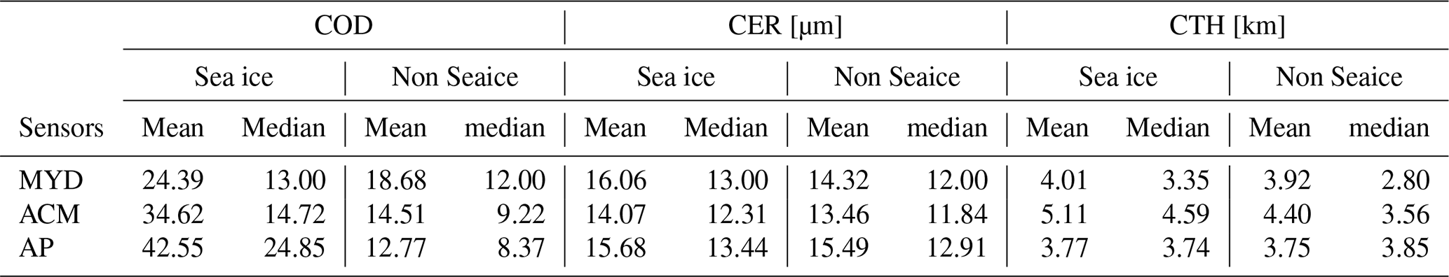
The mean COD for AC was 34.62 and 14.51; for MYD it was 24.39 and 18.68; and for AP it was 42.55 and 12.77 for sea ice and non-sea ice cases, respectively. The optical depth of the retrieved pixels increased in the presence of sea ice for all sensors. The results disagree with the findings of Frey et al. (2018) and Palm et al. (2010), which concluded that clouds were more frequent, and cloud optical depth tends to be higher over ice free regions. While the disagreement could arise from differences in latitude range and the limited temporal scope of our dataset compared to the multi-year analyses Frey et al. (2018) and Palm et al. (2010). It is hypothesised that the difference is due to two effects both originating in flaws of the retrieval algorithms: 1 – sea ice (with no associated cloud) is misidentified as cloud; this could be the cause of the spike in observations with greater than 100 COD over sea ice, and 2 – the albedo of sea ice used in the retrieval algorithms introducing a systematic positive COD bias. It is difficult to define an accurate sea ice albedo; a systematic underestimation of the albedo could cause the optical depth of clouds to be overestimated.

In the comparison of CTH and CER between sea ice and non-sea ice cases, the differences for AP are small (0.2 µm for CER and −0.02 km for CTH). The MYD and AC products also show small positive differences in CER (≈1 µm) over sea ice. For non sea ice cases, the CTHs are 0.09 km (MYD) and 0.6 km (AC) lower than sea ice cases. Although CER and CTH exhibit positive differences, these were much smaller than the differences observed for COD.

The seasonality of the COD, CER, and CTH anomalies over sea ice was also examined. We observed that the disagreement between retrievals over sea ice and non sea ice is higher in JJA, where sea ice cases show (not shown here) lower COD and CTH values. COD values remain below 50 for AC and MYD and below 80 for AP across all seasons, with generally lower values over sea ice in winter (JJA). CER distributions are relatively consistent across seasons, ranging from 0–35 µm for AP, 5–65 µm for MYD, and 5–45 µm for AC. Seasonal variation is more evident in CTH: low clouds (less than 2 km) dominate for MYD and AP in JJA and for all three sensors in SON, while DJF and MAM show a greater presence of mid-level clouds (3–6 km), though low clouds remain prominent for MYD and AP. It can be concluded that in the case of CTH and CER, the seasonality is not an important factor, while for COD, the seasonality and presence of sea ice are important factors in the retrieval of the product.

5 Summary and Conclusion

In this study we have compared and validated the cloud property retrievals from merged CloudSat-CALIOP (CC) and MODIS-AQUA (MYD), AVHRR CMSAF (CLARA A3), and AVHRR PATMOS-x (V6) over the SO for monthly (L3) and instantaneous (L2) data. The results showed significant differences in cloud top height, cloud fraction (cloud mask), optical depth, thermodynamic phase, and cloud effective radius.

For the Level 3 comparison, when compared to CALIOP CTHs for the top layer, we found that MODIS generally tends to underestimate the CTHs and AVHRR CMSAF tends to overestimate the CTH. The monthly observations of the CTHs revealed significant biases and poor correlation. The observed cloud fraction for passive sensors was higher than for active sensors, especially towards the mid-latitudes (40–60° S). In comparison to CALIOP CFC, the AVHRR CMSAF CFC was 20 % greater and the MODIS CFC was 10 % greater. On the other hand, over the high latitudes (60–70° S), MODIS CFC was 10 % less compared to CALIOP CFC. We observed that over Antarctica, CALIOP CFC was 10 % greater than MODIS CFC and 20 % greater than AVHRR CMSAF. When comparing the cloud fraction for liquid clouds with CALIOP, MODIS has an overall lower cloud cover, while AVHRR CMSAF has a lower cloud cover over the land and a higher cloud cover over mid-latitudes. During the seasonal analysis, we observed that austral summer (DJF) has lower bias and higher correlation than other seasons, while winter has higher bias and poorer correlation for CTH comparison. It can be concluded that over the Antarctic coast CALIOP L3 cloud properties retrievals, have a positive bias with both MODIS and AVHRR CMSAF. However, over the mid-latitude, AVHRR CMSAF overestimates the cloud properties when compared to CALIOP.

An extensive analysis of L2 passive sensor (AVHRR CMSAF, MODIS, and AVHRR PATMOS-x) observations against active sensor (CLOUDSAT-CALIOP merged) observations, was carried out in order to identify the factors contributing to the bias in cloud property retrievals. The presence of multilayer clouds, sea ice, and cloud mask were some of the factors analysed.

In the case of the CTH analysis, without the 0.5 COD threshold, a mean absolute bias of 0.65 km (AVHRR CMSAF), 1.03 km (MODIS), and 1.27 km (AVHRR PATMOS-x) was observed for single-layer cloud scenes cases. This mean bias increased to 1.87 km (AVHRR CMSAF), 3.25 km (MODIS), and 3.30 km (AVHRR PATMOS-x) for multilayered cloud scenes. Hence, we can conclude that the passive sensor MAE against the active sensor for multilayer cases is 3–4 times the corresponding MAE for single-layer cases and 2 times MAE for the overall year. The bias can also be attributed to the retrieval algorithm differences, COD of the layers, and sensitivity of sensors to the cloud.

The comparison of L3 cloud top height, with MODIS underestimating and AVHRR CMSAF overestimating relative to CALIOP, agrees with the L2 comparisons of passive sensor CTHs against CLOUDSAT-CALIOP merged data. This consistency indicates that L3 biases are a cumulative result of the underlying retrieval limitations of L2 retrievals.

The second major finding of this study, the cloud mask comparison revealed varying levels of agreement between passive and active sensor observations, with AVHRR PATMOS-x showing relatively lower skill. More than half of the observations for AVHRR PATMOS-x (KSS=0.43) show disagreement, likely due to its different spatial resolution from other sensors. In the case of sea ice-classified pixels, the KSS rates are lower, indicating the influence of sea ice on the cloud observation.

In the comparison of CER, it was observed that the disagreement between the passive sensors was slightly higher in presence of multilayer clouds. In single-layer cases, the liquid water phase dominates for MODIS and AVHRR CMSAF. The AVHRR PATMOS-x shows more ice phase for single-layer clouds than other passive sensors, with two peaks in the CER at 10 and 30 µm. The analysis of CER, COD, and CTH in relation to the sea ice mask revealed that the presence of sea ice plays an important role in retrieval of COD.

The comparison and validation conclude that all passive sensors showed cloud property differences when compared with CloudSat-CALIOP and when compared with each other, agreement and disagreement. The AVHRR CMSAF performs well for CTH retrievals, but in multilayer scenarios, the correlation is lower. Similarly, MODIS is generally good at retrieving CTH, but in multilayer clouds, it has higher negative bias when compared to AVHRR CMSAF. The AVHRR PATMOS-x retrievals exhibited the lowest correlation in both the overall CTH and the multilayer and single-layer cases. The agreement between the cloud thermodynamic phase and the active sensor is reduced for AVHRR PATMOS-x. Although MODIS has more channels and hence more information content compared to other retrievals, it does not perform better than AVHRR CMSAF with a neural network retrievals.

The bias is affected by the multilayer structure of the clouds, problems with temperature profile inversion, incorrect identification and classification of the thermodynamic phase. The agreement for single-layer cloud retrieval is higher than the agreement for multilayer classified cloud retrieval. This suggests that we need to invest more effort into improving multilayer retrieval issues, especially over the SO where the cloud properties are very different from those in other areas.