Analysis of convective cell evolution with split and merge events using a graph-based methodology

Convective storms are associated with several hazards, including heavy rainfall, hail, and lightning, which pose severe risks to society. While the nowcasting (i.e., short-term forecasting from 5 min to 6 h) of storm locations has been extensively studied, nowcasting storm development remains a challenge. Nowcasting rapid, non-linear convective storm evolution requires finding connections between observations and storm evolution and representing them in the nowcasting model. Convective cell identification and tracking algorithms are commonly used for nowcasting and analysis of convective storms. This analysis is complicated by the splits and merges that occur in the cell tracks, either due to the physical processes or data quality issues. Consequently, the splits and merges are often excluded from the analysis. Here, we present a methodology for analyzing cell development around time of interest that explicitly includes the splits and merges in the analysis. The time of interest can be the time when the nowcast is created or the occurrence of some fingerprint of meteorological processes, for example, Z_dr columns. We represent the cell tracks as directed graphs where we select event nodes to represent the times of interest. For each event node, a subgraph of related cells from both the past and future of the event node is selected. We propose rules for selecting the subgraphs with the aim of retaining the available information in the subgraph at each time step. Once selected, the cell features in the subgraphs are aggregated into time series for analysis. We demonstrate the methodology through case studies of convective storms with Z_dr column features signalling updrafts and apply it to analyze split and merge events using three years of warm-season (MJJAS) operational radar data from the Swiss national weather radar network, with a focus on the total rainfall amount produced by the cells. Splits and merges occur in 7.2 % of all identified cells, and are more frequent in cells with larger vertically integrated liquid (17.9 %) or containing Z_dr columns (11.7 %). Typically, cell mergers are associated with growth in total rainfall and cell area, and cell splits are associated with decrease in total rainfall.

1 Introduction

Convective storms are associated with several meteorological phenomena, such as heavy rainfall, lightning, hail, and strong winds, that pose severe hazards to society. Because convective storms tend to evolve rapidly, producing accurate and timely hazard forecasts and warnings, such as flash flood warnings, requires short-term forecasting with lead times ranging from 5 min to 6 h, i.e., nowcasting (World Meteorological Organization, 2017). The nowcasting of convective storms in operations is a challenging task. Although the development stages of convective storms are relatively well understood through modelling and observational case studies (Brooks et al., 2018), acquiring and representing the knowledge of the storm evolution from observations for use in real-time operational nowcasting models remains a challenge. Furthermore, the rainfall amounts produced by the storms are expected to increase due to climate change, emphasizing the need for accurate short-term forecasting and warning systems (Rädler et al., 2019; Taszarek et al., 2021; Utriainen et al., 2025).

Weather radar measurements are particularly well suited for analyzing and nowcasting convective storms because of their high spatial and temporal resolution (e.g., 100 m to 1 km and 1 to 5 min), the wide spatial coverage provided by national radar networks in many countries, and their ability to estimate surface rainfall more effectively than satellites (Li et al., 2024; De Luca et al., 2025). In addition to estimating rainfall, radar measurements can provide other information relevant to the evolution of the storms. In recent years, several fingerprints of convective storm processes have been identified in polarimetric radar measurements. For example, differential reflectivity (Z_dr) columns have been shown to be proxies for updrafts (Kumjian et al., 2014). These fingerprints can precede the intensification of the storms or the onset of hail or heavy rainfall, and thus may have potential for improving the nowcasts (Picca et al., 2010; Kumjian et al., 2014; Snyder et al., 2015; Kingfield and Picca, 2018; Van Den Broeke, 2017; Wilson and Broeke, 2022).

Representing the convective storms as objects, i.e., convective cells, provides a convenient approach for associating the temporal evolution, different fingerprints of the convective storm processes, as well as storm-related hazards into a single conceptual model. These phenomena often manifest at scales significantly larger than a single radar pixel or through different modalities, such as binary detection of lightning versus continuous measurement of rainfall intensity. Consequently, linking these phenomena with grid-based approaches, which treat radar pixels individually, is challenging. However, handling these different properties together becomes simpler when the convective storms are represented as objects combining all radar pixels within the object (Rossi, 2015).

Figure 1 Overview of the presented analysis methodology.

Convective cells are usually identified with contour-based methods, where the cells are defined as contiguous areas exceeding a threshold aimed to differentiate between stratiform and convective rainfall (e.g., 35–40 dBZ in radar reflectivity), with possibly some post-processing applied to further refine the extent of the identified cells (see e.g., Steiner et al., 1995; Lakshmanan et al., 2003; Hering et al., 2004; Muñoz et al., 2018). Depending on the targeted phenomena, other identification criteria may also be used, such as image texture (Guyot et al., 2023). Once identified, cells at consecutive time steps are matched to each other based on some algorithm-specific criteria, e.g., similarity or distance between the cells, to form cell tracks that describe the temporal evolution of the cells. A variety of algorithms have been developed for cell identification and tracking from weather radar observations (e.g., Dixon and Wiener, 1993; Johnson et al., 1998; Handwerker, 2002; Lang, 2002; Hering et al., 2004; Kyznarová and Novák, 2009; Muñoz et al., 2018; Skinner et al., 2018; Hu et al., 2019; Zan et al., 2019; Hou and Wang, 2017; Raut et al., 2021; Fluck et al., 2021; Shi et al., 2024). The cell tracks can be used to study convective storm evolution and climatology in radar data or simulations (e.g., Kyznarová and Novák, 2009; Liu and Li, 2016; Hu et al., 2019; Feldmann et al., 2021; Oue et al., 2022; Wilhelm et al., 2023; Tuftedal et al., 2024; Gupta et al., 2024); study convective initiation (Merk and Zinner, 2013); nowcast future locations of the cells (Dixon and Wiener, 1993; Rossi et al., 2015; Wang et al., 2023); estimate and nowcast hazards related to the cells (Rossi et al., 2012; Tervo et al., 2019; Esbrí et al., 2023; Heinselman et al., 2024); or evaluate the forecast skill of grid-based nowcasting systems (Ritvanen et al., 2025b). Historically, most attention has focused on nowcasting the location of convective cells with extrapolation methods, whereas nowcasting their evolution has remained a challenge.

A major challenge in the analysis of convective cell evolution through cell tracking is the occurrence of splits and merges in the tracks when a cell has multiple parent cells or child cells instead of a single cell. Splits and merges can be caused by two separate factors. First, splitting and merging are genuine meteorological processes observed in convective storms, driven by various forcing mechanisms (Bluestein et al., 1990; Westcott, 1984). Additionally, horizontal motion can cause multiple identified cells to converge into one or, similarly, one cell to multiple, especially if the cells are defined to contain areas larger than only the convective core of the storm. We refer to these as true merges and splits. Second, merges and splits can result from inconsistencies in the identification algorithm or data artefacts (e.g., strong attenuation), which may cause a cell to be artificially identified as multiple cells, causing a split or merge to be mistakenly identified in the tracks, or from overly permissive matching criteria in the cell tracking algorithm. Even though the impact of these artificial splits and merges can be mitigated by data quality control and fine-tuning of the cell identification and tracking algorithms (Lamer et al., 2023), true splits and merges are inherent features of storm evolution and excluding them from analysis can remove useful information. Furthermore, the separation between true and artificial splits is not always obvious; in some situations, the evolution of the cells can be so chaotic that even experienced meteorologists may find it difficult to visually identify the splits or merges.

Most cell tracking algorithms provide information on splits and merges, but these events lead to complex track structures that complicate analysis of the evolution. A common approach when analyzing the tracks is to determine a “most representative” path through a track, typically based on minimizing variation in some attribute, such as radar reflectivity factor inside the cell, across the cell track (Liu and Li, 2016; Fluck et al., 2021; Feng et al., 2022; Cheng et al., 2024; Tseng et al., 2025; Bournas and Baltas, 2024; Ritvanen et al., 2025b). This approach assumes that a “good” cell track should preserve storm-related attributes (Lakshmanan and Smith, 2010), and thus minimizing variability in the attributes yields the track that best describes the storm. In this approach, during a split, the original cell track is continued in the “most representative” cell among the multiple potential child cells, while other cells initiate new tracks. Similarly, in a merge, the track of the parent cell most similar to the new cell continues, and other tracks are terminated. Another commonly used approach is to simply exclude any tracks containing splits or merges from the analysis (Lamer et al., 2023; Wilhelm et al., 2023; Tuftedal et al., 2024).

The “most representative” path approach is useful for analysing the cell tracks for long time periods or full cell life cycles. In such cases, favouring long, stable cell tracks is most likely to produce good results. However, when we want to analyze the evolution of the cells in a limited time window related to some event, or to use the analysis for nowcasting purposes, such as to predict the immediate development of the cells, this approach is less suitable. In forecasting, the future state of the cells is not known, so it cannot be used for determining the “most representative” path. Rather, we want to gather all available information in a short time window surrounding the analysis time that could contain information useful for predicting the development of cells. Furthermore, the importance of the splits and merges to the analysis depends on the application. For example, in the dataset analyzed in this study (see Sect. 2.1), the fraction of all identified cells with splits or merges, i.e., cells with multiple parent or child cells, is 7.2 %; however, 11.7 % of the identified cells that are associated with a Z_dr column feature and 17.9 % of cells where the maximum vertically integrated liquid (VIL) inside the cell is at least 20 kg m⁻² have splits or merges. Thus, especially if the analysis is focused on these cells, it is sensible to include the split and merge branches of the cell tracks in the analysis.

A logical approach to explicitly include the splits and merges in the analysis is to represent the cell tracks as spatio-temporal graphs (Liu et al., 2016; Hou and Wang, 2017). In this approach, each cell is represented as a node, and the temporal connections between cells at consecutive time steps as edges in the graph. Split cells are nodes with multiple out-going edges and merge cells are nodes with multiple incoming edges. In this approach, defining the “most representative” path is not necessary and all branches of the tracks can be accounted for together. Spatio-temporal graphs have been used in other fields for geospatial data analysis (e.g., Liu et al., 2019; Wang et al., 2020; Xue et al., 2019b). However, compared to many other datasets, cell tracks present challenges due to their (usually) large amount and the variability of the tracks, ranging from short-lived isolated cells to large, long-lived organized convective systems. The variability of the cell track graphs makes it challenging to define isomorphisms (transformations) between the cell track graphs that are often used in quantitative graph analysis (e.g., Yan et al., 2016). Previous studies applying the cell track graph approach have largely focused on quantifying split and merge statistics, e.g., their counts or spatial distribution, or on full storm lifecycle without emphasizing the splits or merges (Liu et al., 2016; Liu and Li, 2016; Yin et al., 2022; Xue et al., 2019a).

However, to analyze and predict the development of cells in a short time window surrounding some specific event (such as the occurrence of a Z_dr column feature or the nowcast creation time), we need to be able to extract the parts of the cell track graphs that are relevant for the analysis; the question of how to do this systematically has not been addressed by previous studies. In this study, we develop a methodology that extracts the cells that are related to any instantaneous event from the cell track graph, enabling quantitative analysis of cell development in relation to the event. The proposed methodology enables analysis of the cell development in the presence of splits or merges in the cell track. The workflow is illustrated in Fig. 1, and the terminology used in the study is listed in Table 1. First, cell tracks are represented as directed graphs. Then we select event nodes that are of interest to the analysis from the cell track graphs. For each event node, we select a subgraph of related cells from both the past and future of the event node. We propose the selection rules for the subgraphs with the aim of retaining the available information in the subgraph at each time step. Once selected, these subgraphs are aggregated into time series for each event node, which can then be analyzed to assess the impact of the event node on convective cell development.

We demonstrate the methodology through case studies, as well as by applying it to post-event analysis of a dataset consisting of split and merge events using three years of warm-season (May–September) operational radar products from the Swiss weather radar network. The cells in the dataset were identified for the purpose of analyzing factors impacting convective rainfall. We present statistics on the splits and merges in the dataset and discuss their significance to the analysis of the cell tracks. Then we analyze the impact of the splits and merges to the total rainfall in the cells and the cell area using the methodology.

The rest of this article is structured as follows. Section 2 describes the methodology in detail, as well as the data used in the analysis. Section 3 presents two case studies demonstrating the methodology, and Sect. 4 discusses the results of applying the methodology to the dataset of split and merge events. Finally, Sect. 5 summarizes the article.

Table 1 Description of terms used in the study.

2 Methodology and data

2.1 Radar data

In this study, we use weather radar data from the Swiss national weather radar network. Mainly, two different radar products are used: firstly, the convective cells are identified from vertically integrated liquid (VIL; Greene and Clark, 1972; Hu et al., 2019; Esbrí et al., 2023; Tuftedal et al., 2024) and, secondly, the rainfall amount inside the cells is determined from the radar-only quantitative precipitation estimation (QPE) product (Germann et al., 2006, 2022). Both radar products are produced operationally by MeteoSwiss with a temporal resolution of 5 min and a spatial resolution of 1 km as a composite product of 5 C-band radars on a Cartesian grid. The size of the products is 710 × 640 km, and the product domain is demonstrated in Fig. 3. The dataset used in the analysis presented in Sect. 4 is extracted from May to September from the years 2021–2023.

The VIL, in units of kg m⁻², is calculated by integrating radar reflectivity observations in a vertical column (Greene and Clark, 1972):

$$\begin{array}{}\text{(1)}& \mathrm{VIL}=\mathrm{3.44}\times {\mathrm{10}}^{-\mathrm{6}}\underset{h_{\mathrm{bottom}}}{\overset{h_{\mathrm{top}}}{\int }}{Z}^{\mathrm{0.57}}\mathrm{d}h\end{array}$$

where h is the height in m, h_bottom and h_top are the echo base and top heights, respectively, and Z is the radar reflectivity in linear units of millimetres to the sixth power per cubic meter. The minimum non-zero value of the VIL product is 0.5 kg m⁻², and the product is stored in an 8-bit format with a resolution of 0.5 kg m⁻².

The rainfall product is created from radar reflectivity observations using the Z−R relation Z=316R^1.5 where the radar reflectivity Z is in linear units of mm⁶ m⁻³, and the rainfall rate R is in units of mm h⁻¹ (Germann et al., 2006; Joss et al., 1998). The data are further processed to remove ground clutter and non-meteorological echoes, correct for visibility and vertical profile of reflectivity, and correct for bias compared to rain gauge measurements (Germann et al., 2006), before being stored in an 8-bit format. Furthermore, to avoid overestimation in the presence of hail, rain rates are saturated at approximately 120 mm h⁻¹ (approximately 56 dBZ). From the rainfall product, we determine the total rainfall inside the cells as the volume rain rate (RVR; in units of m³ h⁻¹) that is the integrated rain rate over the cell area at a given time step. The definition of volume rain rate is similar to what was used, for example, by Rosenfeld (1987); Hu et al. (2019); Feng et al. (2018) and Ritvanen et al. (2025b).

Additionally, in the case studies in Sect. 3, we use the Z_dr column height (Z_drC) determined from the radar observations to demonstrate the impact of splits and merges for the continuity of Z_drC signals in the convective cells. Z_dr columns are vertically contiguous areas of high Z_dr (in this case, Z_dr≥1 dB) above the environmental 0 °C level that can be used as a proxy for updrafts in convective storms (e.g., Illingworth et al., 1987; Kumjian et al., 2014; Picca et al., 2010). For more details about the Z_drC data, refer to Snyder et al. (2015); Aregger et al. (2025) and Appendix B.

2.2 Cell track graph construction

The first step of the presented analysis methodology involves identifying and tracking the convective cells within the data. Once the cells are tracked, the cell tracks are constructed into graphs. In the graph construction, each distinct cell track is presented as a directed simple acyclic graph $\mathcal{G}=(V,E)$ where V represents the nodes (cells) belonging to the graph and E represents the edges (temporal connections) between the nodes produced by the tracking algorithm. More specifically, the nodes are defined as a set $V=\mathit{\left\{}\right(t,\mathrm{id},A\left)\mathit{\right\}}$, where t is the time step where the cell was identified, id is an identifier that uniquely identifies the cell at time step t, and A is a set of attributes associated with the cell (e.g., the volume rain rate or the cell area). The edges are defined as a set $E\subseteq \mathit{\left\{}\right(v_{\mathrm{1}},v_{\mathrm{2}})=((t_{\mathrm{1}},{\mathrm{id}}_{\mathrm{1}},A_{\mathrm{1}}),(t_{\mathrm{2}},{\mathrm{id}}_{\mathrm{2}},A_{\mathrm{2}}))\mid v_{\mathrm{1}},v_{\mathrm{2}}\in V\mathrm{and}{t}_{\mathrm{1}}<t_{\mathrm{2}}\mathit{\}}$, i.e., the connections between two nodes v₁ and v₂ in the cell track, defined in an order so that v₁ occurs before v₂. Furthermore, for each node v, we can construct the set of parent nodes (mathematically known as in-neighbourhood) $N^{-}\left(v\right)=\mathit{\{}u\mid (u,v)\in E\mathit{\}}$, and the set of child nodes (out-neighbourhood) $N^{+}\left(v\right)=\mathit{\{}u\mid (v,u)\in E\mathit{\}}$. Using these definitions, we can define:

• a merge cell as a node with more than one parent but at most one child: $\left|N^{-}\right(v\left)\right|>\mathrm{1}$ and $\left|N^{+}\right(v\left)\right|\le \mathrm{1}$,

• a split cell as a node with more than one child but at most one parent: $\left|N^{-}\right(v\left)\right|\le \mathrm{1}$ and $\left|N^{+}\right(v\left)\right|>\mathrm{1}$,

• a merge-split cell, formed from multiple merging cells and splitting into multiple cells at the next time step, as a node with both more than one parent and more than one child: $\left|N^{-}\right(v\left)\right|>\mathrm{1}$ and $\left|N^{+}\right(v\left)\right|>\mathrm{1}$

• a new (born) cell as a node with no parents but at least one child: $\left|N^{-}\right(v\left)\right|=\mathrm{0}$ and $\left|N^{+}\right(v\left)\right|>\mathrm{0}$, and

• a terminal (dying) cell as a node with at least one parent but no child cells: $\left|N^{-}\right(v\left)\right|>\mathrm{0}$ and $\left|N^{+}\right(v\left)\right|=\mathrm{0}$.

Each cell track graph consists of all identified cells connected to each other through some other cell in the track, either in the past or future, allowing the cell track graphs to cover arbitrarily many consecutive time steps. Because of this, a single cell can only be part of one cell track graph. However, multiple cell track graphs originating from different cells can co-exist at the same time steps. Here, the methodology is applied to historical data; if used in real-time analysis or nowcasting, the cell track graphs need to be reconstructed each time after new observation time steps are added to the dataset.

Note that the methodology described here is independent of the identification and tracking algorithms, provided that the tracking algorithm supplies information on splits and merges occurring in the cell tracks. Additionally, any potential spatial connections between the cells at one time step, such as, spatial clustering or multiscale cell identification (e.g., Lakshmanan et al., 2003; Hou and Wang, 2017), are not considered in this study and are left for future development. If algorithms that produce spatial connections, such as clusters, are used, the clusters or a single level of the multiscale cells could replace the convective cells in the graphs. As with any cell-based analysis, the cell identification and tracking algorithms impact the results obtained from the analysis, so the algorithms and objects used in the graphs should be selected so that they describe the phenomena studied as well as possible.

In this study, the cells were defined for the purpose of analyzing factors impacting convective rainfall in operational weather radar products. The cells are identified from the VIL product using a constant threshold of 1.0 kg m⁻², with a minimum detected cell size of 10 km², and a tracking algorithm based on the algorithms used by Rossi et al. (2012, 2015) and Tervo et al. (2019) is employed. Appendix A describes the cell identification and tracking algorithms.

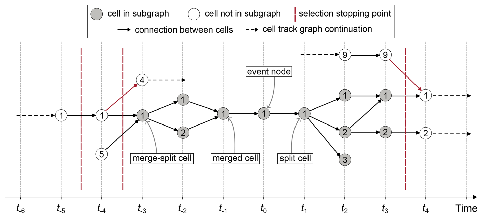
Figure 2 Example of cell subgraph selection from the cell track graph. For the event node labelled 1 at time t₀ the subgraph selection stopping points are presented with dashed vertical lines and cells accepted into the subgraph are coloured as grey. The arrows in the graph represent the temporal connections between the cells.

2.3 Subgraph selection

After the cell track graphs are constructed, the subsequent steps involve selecting the event nodes of interest and extracting the subgraph for each event node using a breadth-first approach (Cormen, 2009). The event nodes should be selected to represent the instantaneous events that are analyzed. In the results presented later in this study, the event nodes include all merge, split, and merge-split cells. Depending on the goals of the study, other criteria for selecting the event nodes could involve, for example, peak in rainfall or the occurrence of certain polarimetric features. For each selected event node, we denote time step of the event node as t₀, the time steps backwards from the event node as $t_{-\mathrm{1}},t_{-\mathrm{2}},\mathrm{\dots }$ , and the time steps forwards after the event node as $t_{\mathrm{1}},t_{\mathrm{2}},\mathrm{\dots }$.

For each event node v, the subgraph is constructed in two stages: backward and forward selection. In backward selection, we select predecessor cells that are connected to the event node, and in forward selection, successor cells that are connected to the event node. An example of the selection is shown in Fig. 2. The selection aims to retain the information at each time step in the subgraph; if information is lost or added at some time step, the selection is stopped. Information here is understood to mean all the observed cell attributes, such as the rainfall in the cells, the cell area, or the presence of Z_dr column features, and their temporal development. In backward selection, information could be lost through splits where some child cells are not in the current subgraph, or added in new cells. In forward selection, new information could be added by a merge where some parent cells are not in the current subgraph. The selection is done so that at each time step either all cells connected to the event node are included in the subgraph, or none of them. The cells belonging to the backward subgraph are denoted as $S_m^{-}\left(v\right)$ and the forwards subgraph as $S_n^{+}\left(v\right)$, where m and n are the maximum number of time steps traversed backwards and forwards, respectively.

Algorithm 1 describes the selection of the cells $S_m^{-}\left(v\right)$ in the subgraph backward from the event node. To select the cells, a backward traversal from the event node is conducted. At each time step $t_{-\mathrm{1}},\mathrm{\dots },t_{-n}$, the parents of all cells that are part of the current subgraph at the previous time step are inspected. In the backward subgraph, two special cases are considered: (1) if the cell splits and (2) if the cell is a new cell.

For splitting cells, the cell is accepted in the subgraph only if all of its child cells are already in the subgraph; otherwise, the cell is not accepted, and the subgraph selection is stopped at the previously inspected time step. For example, in Fig. 2, at t₋₃ cell number 1 is a split cell with both of its child cells (1 and 2 at time step t₋₂) in the subgraph, and thus accepted. However, at t₋₄ cell 1 is a split cell for which one child cell (4 at t₋₃) is not a predecessor of the event node, and therefore, cell 1 at t₋₄ is not accepted into the subgraph. Since information is discarded at time step t₋₄, the subgraph selection is stopped at the previous time step t₋₃.

In the case of new cells, the cell is accepted in the subgraph, but since the new cell contains information that does not exist at the next inspected time step, the subgraph selection is stopped after the time step of the new cell. This is demonstrated in Fig. 2, where at t₋₄, cell 5 is a new cell that would cause the subgraph selection to be stopped after time step t₋₄. Note that in the demonstration in Fig. 2, cell 5 at t₋₄ would not be included due to the split occurring in cell 1, but if that split did not occur, cell 5 would be included, and the subgraph selection would be stopped after t₋₄.

Similarly, Algorithm 2 describes the forward subgraph $S_n^{+}\left(v\right)$ selection. At each time step $t_{\mathrm{1}},\mathrm{\dots },t_m$, the children of all cells that are part of the subgraph at the previous time step are inspected. For the forward subgraph selection, the special cases are the merge cells, which are accepted only if all of their parent cells are included in the subgraph at the previous time step. For example, in Fig. 2, at t₃, cell 1 is a merge whose parent cells are all included in the subgraph, and it is thus accepted. However, for the merge cell 1 at t₄, one parent (cell 9 at t₃) is not a successor of the event node, and hence cell 1 at t₄ would introduce new information to the subgraph and it is not accepted. Not accepting cell 1 at t₄ removed some information at t₄, so the entire time step t₄ must be disregarded, and the subgraph selection is stopped after t₃. Note that in the forward subgraph selection terminal (dying) cells do not stop the subgraph selection (as opposed to new cells in the backwards subgraph selection), as they do not introduce new information into the subgraph.

After both the backward and forward subgraphs have been constructed, the full subgraph for the event node v can be defined as a graph ${\mathcal{T}}_{n,m}\left(v\right)=\left(S_{n,m}\right(v),C_{n,m}(v\left)\right)$ where the nodes are defined as $S_{n,m}\left(v\right)=S_n^{-}\left(v\right)\cup \mathit{\left\{}v\mathit{\right\}}\cup S_m^{+}\left(v\right)$ and the edges $C_{n,m}\left(v\right)=\mathit{\left\{}\right(x,y)\in E\mid x,y\in S_{n,m}(v\left)\mathit{\right\}}$, where E are the edges in the cell track graph.

The algorithms presented here can be applied to tracks in real-time, i.e., without information on the future development of the tracks. Using incomplete cell tracks can impact the composition of the cell track graphs, as the cell tracks could become connected at a later time. However, the only limitation for subgraph selection and subsequent analysis would be a restriction on how many time steps forward the subgraphs can be selected (if those time steps do not exist in the data). Because the forward selection of the cells in the subgraph at one time t_i does not depend on the next time step t_i+1, the forward selection could be done iteratively as new time steps are observed without changing the selections at previous time steps.

2.4 Subgraph development analysis

After subgraph construction, each event node v is represented by a subgraph with possibly multiple cells at the time steps $t_{-n},\mathrm{\dots },t_{-\mathrm{1}},t_{\mathrm{1}},\mathrm{\dots },t_m$ (note that at t₀, the only cell is the event node v). The subgraphs are aggregated at each time step to produce a single time series centered at the time of each event node.

The method of aggregation over cells at one time step depends on the attribute studied, and should be selected so that the resulting variable is sensible. The volume rain rate and area of the cells are used in this study; these variables are summed over the cells at each time step to obtain estimates for the total volume rain rate and area of the subgraph. For variables where summing is not appropriate, such as mean or maximum rain rate, values can be aggregated by averaging or taking the maximum or minimum. The average can also be weighted by some attribute, such as cell area.

For any aggregated variable x_i, where i is the time step for which the variable is calculated, the relative change compared to time step t₀ is defined as

$$\begin{array}{}\text{(2)}& Q{x}_i={\displaystyle \frac{\mathrm{\Delta }{x}_i}{x_{\mathrm{0}}}}={\displaystyle \frac{x_i-x_{\mathrm{0}}}{x_{\mathrm{0}}}}\end{array}$$

Note that with this definition, the relative change at t₀, Qx₀, is always zero, but the variable x₀ is not. In fact, Eq. (2) is not defined if x₀=0, and the relative change Qx_i can be misleading if x₀ is very small. For variables where very small or zero values are possible, it is recommended to either apply some transformation or redefinition of the variable or also study the absolute difference Δx_i.

Finally, information on subgraph development can be obtained from the values of x_i or Q_i. Note that the number of subgraphs at each time step $t_{-n},\mathrm{\dots },t_m$ is likely different, with the maximum number of samples existing at t₀, because every subgraph exists at least at time t₀ (event node time step) but not necessarily at the previous or next time steps. Therefore, results should be interpreted with care; the value Qx_i describes the relative change only in the samples of subgraphs for which cells could be selected from t₀ to t_i.

Figure 3 Overview of the rainfall field for the case studies at (a) 7 June 2022 17:35 UTC and (b) 13 July 2021 09:35 UTC. The magenta boxes indicate the area shown in (a) Fig. 4 and (b) Fig. 5. The crosses indicate radar locations, and the distance between the grid lines is 100 km.

3 Case studies

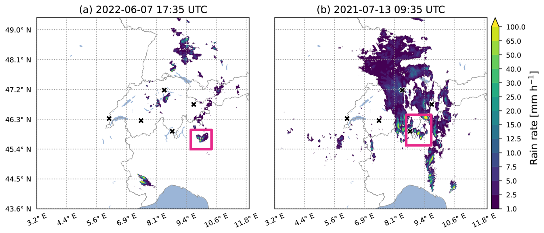
We demonstrate the methodology using two case studies of rainfall events with merge-split cells, one from 7 June 2022, and another from 13 July 2021. An overview of the rainfall fields at the case study times are shown in Fig. 3.

The first case study subgraph on 7 June 2022, shown in Fig. 4, occurs as a part of a cell track existing between 16:45 and 19:50 UTC, consisting of an isolated convective system with at most three cells identified at any time. The merge-split event node, for which the subgraph is constructed, occurs at 17:35 UTC when the two cells identified at 17:30 merge into one cell. This cell then splits into two cells at 17:40. After this, the cell labelled 2 continues to grow in both cell area and mean rain rate. The other cell, labelled 1, begins decaying and splits into two more cells at 17:50, which are no longer identified after 18:00. The opposing development of the two branches of the subgraph after the event node, one growing and one decaying, is captured in the time series graphs shown in Fig. 6b–d. Additionally, Fig. 6f shows the impact of the decaying subgraph branch on the total cell area: although the total cell area is consistently larger than at t₀, the relative change in total cell area decreases after 17:45 due to the decaying branch, while the relative increase in the volume rain rate, dominated by the growing subgraph branch, is much higher after 17:45.

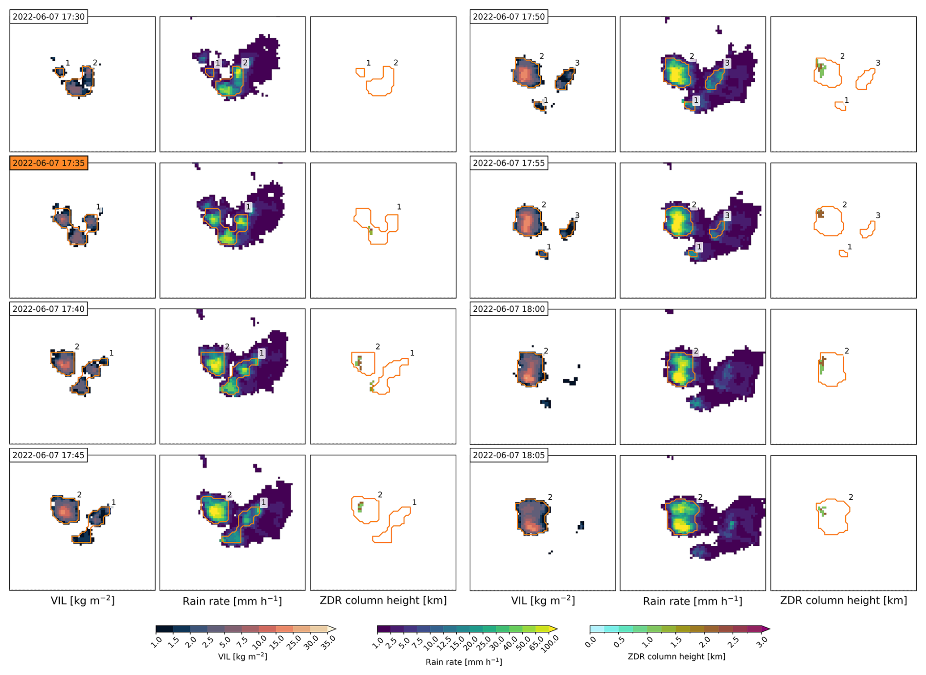
Figure 4 Time series of the case study on 7 June 2022 17:30–18:05 UTC. The t₀ time step (orange color background) is 17:35 UTC. For each time step, the left panel shows the vertically integrated liquid (VIL) the middle panel the rain rate, and the right panel the Z_dr column height fields. Cells outlined with orange are part of the case study subgraph, with the labels corresponding to the numbers in Fig. 6a–f. The panels show an area of approximately 70 × 65 km.

The benefit of accounting for splits and merges in the analysis of even such a simple system is best observed when studying the Z_drC signature in the cells (see Fig. 4). The Z_dr column first appears at 17:35 (in the event node) but is observed in the area of the cell that later splits into the decaying branch (labelled as 1) of the subgraph. In this decaying branch, the Z_dr column is observed only once more at 17:40. However, in the other branch, the Z_dr column feature is observed at all time steps between 17:40 and 18:05. Therefore, if the cell track were cut at the split occurring after 17:35 by defining the “most representative” path through the track (bold lines in Fig. 6b–e and h–l), the observed Z_drC time series (Fig. 6f) for the growing branch of the subgraph (labelled 2) would not be complete, and the first time step at which the Z_dr column is detected would be delayed.

The second case study, shown in Fig. 5, involves a merge-split event node from 09:35 UTC on 13 July 2021. This case study occurs on a day with significant convective activity in the domain. The case study event node is a part of a cell track that occurs between 08:25 and 10:40 UTC, with several other cell tracks in the surrounding area. As seen in Fig. 5, the merge-split event consists of two cells, originally initiated independently, merging at 09:35 and then immediately splitting into two cells at 09:40. After this split, both branches of the subgraph split again after 15 min. Fig. 6l shows that before the merge-split, both the total volume rain rate and area were increasing, mainly driven by growth in the cell labelled as 1. Peak values in total volume rain rate and area were obtained at 5–10 min after the event node, after which both begin decreasing as the cells decay.

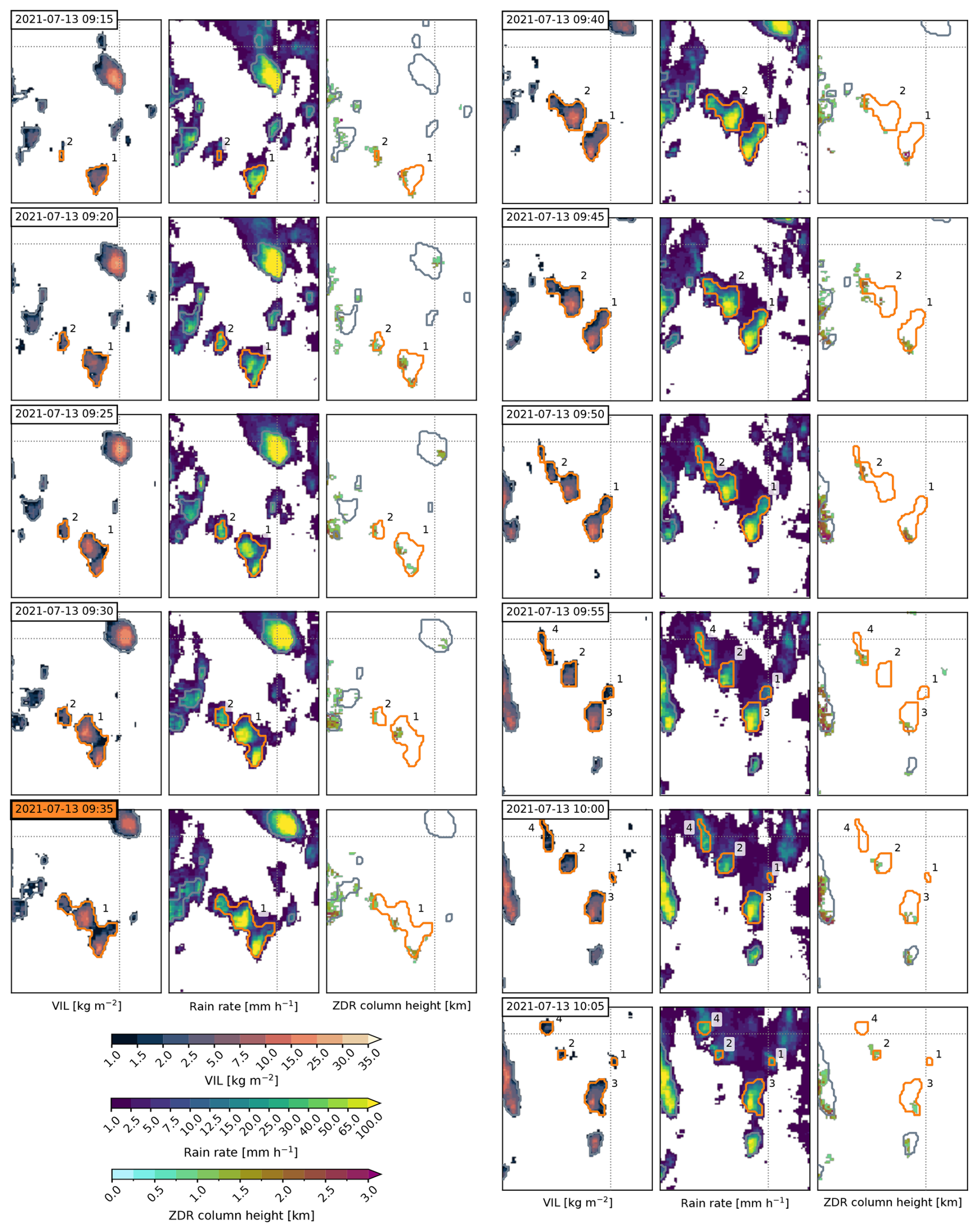
Figure 5 Time series of the case study on 13 July 2021 09:15–10:05 UTC. The t₀ time step (orange color background) is 09:35 UTC. For each time step, the left panel shows the vertically integrated liquid (VIL), the middle panel the rain rate, and the right panel the Z_dr column height fields. Cells outlined with orange are part of the case study subgraph, with the labels corresponding to the numbers in Fig. 6g–l. Cells outlined with grey are cells identified in the area that are not part of the case study subgraph. The panels show an area of approximately 85 × 100 km.

Similar to the first case study, the benefits of considering splits and merges in the analysis are particularly evident in the Z_drC (Fig. 5). If the “most representative” branch were selected at each split or merge event cell for analysis, and other branches considered either new or terminated, the Z_drC signal, which now appears continuously through the whole subgraph (Fig. 6k), would be scattered across multiple tracks, and the full extent of the signal could easily be lost in the analysis. This would happen, in this case study, regardless of the method used to determine the “most representative” path through the cell track.

Even though the cell behaviour, including splits and merges and the exact time at which they are observed, clearly depends on the input data used, as well as the identification and tracking algorithms and their parameters, in this case study the splits and merges cannot be removed completely by algorithm design. For example, visually, the cell labelled 1 at 09:15 (Fig. 5) splits into two cells. Here the split is observed at 09:40, while some identification algorithm may have observed it earlier; however, it can be regarded as a true split. Thus, if we are interested in the development of the cell labelled 1 at 09:15 or the cells resulting from the split in a short time window, analysing the whole track together, including the split, provides the most information.

Figure 6 For the two case studies, (a, g) graph diagrams of the case study subgraphs, and time series of (b, h) cell area, (c, i) cell mean rain rate, (e, j) volume rain rate, (e, k) median Z_dr column height, and (f, l) relative change from t₀ time step in total volume rain rate and cell area. In (a) and (g), the orange-outlined node is the merge-split event node that the subgraph is selected for. In the time series (b)–(e) and (h)–(k), the orange dashed vertical line shows the t₀ time step, and the bold lines indicate the “most representative” cell track that would be obtained by continuing the track of the cell with the largest area at each split or merge. Note that some cells have no values for median Z_dr column height which causes parts of the cell tracks to be missing in panels (e) and (k).

4 Analysis of split and merge events

Next we apply the presented methodology to analyze the split and merge events in the 3-year dataset. To extract the dataset, we first identified and tracked convective cells in the radar data from May to September during 2021 to 2023. Cell track graphs were constructed for all cell tracks that lasted at least 10 min (i.e., two time steps). Details of the cell identification and tracking algorithms used in the study are provided in Appendix A. From this dataset, cells splitting at the next time step (split events), cells formed by a merge (merge events), and cells formed by a merge and splitting at the next time step (merge-split events) were selected as the event nodes, and a subgraph was extracted for each event node. The following section describes the split, merge, and merge-split events, and then investigates the convective cell development related to these events.

Note that, as with any cell-based analysis, the statistics and results presented are dependent on the selected cell identification and tracking methods and their parameters, as well as the data to which the algorithms are applied (e.g., climatology or data processing algorithms). Thus, the aim is not to present universal results about splits and merges, but rather to discuss factors that should be considered when analyzing the cell tracks and how these appear in the dataset. The cell identification and tracking methods used in this study were selected with the aim of analyzing factors contributing to convective rainfall in operational weather radar products; for example, cells are defined at a low VIL threshold to include more rainfall in the cells. This will impact, for example, at which stage the split or merge is identified and can thus impact how they appear in the results. The statistics presented in this section are valid for cell events at single timesteps and do not describe entire cell lifecycles.

4.1 Statistics of splits and merges in the cell dataset

When considering whether to include splits and merges in the analysis of convective cell development compared to selecting only a “most representative” path through the cell tracks, three questions should be considered. First: how many cells have splits and merges; second: among the cells involved in a split or merge events, is there a clear “most representative” cell to be selected, and third: is the impact of the other cells to the development negligible? In this section, we aim to examine these questions by analyzing the number of cells involved in splits or merges and their areas. Because the definition of a “most representative” cell or path through the track depends on the selected algorithm, here we simply use the cell area to characterize the impact of the cells in splits and merges, with the assumption that larger cells would have a greater impact to the event or development than smaller cells. However, this simplified analysis might not be directly comparable with algorithms that define the “most representative” path in the cell track using information from outside the cells involved in splits or merges (such as global features of the cell track; see, e.g., Liu et al., 2016).

In the dataset, the fraction of split or merge cells is 7.2 % (53 059 out of 735 163) from all identified cells, with splits and merges comprising 3.0 % (21 951) and 3.2 % (23 391) of the dataset, respectively, and merge-split cells 1.0 % (7717). However, the fraction of splits and merges increases when looking at more intense cells. In cells with maximum VIL inside the cell at least 20 kg m⁻², the fraction of splits or merges is 17.9 % (6770 out of 37 786). Furthermore, in cells associated with a Z_drC feature, the fraction of splits or merges is 11.7 % (21 364 out of 181 835). Thus, the impact of splits and merges to the analysis depends on the selection of the cells that the analysis focuses on.

One factor describing the complexity of a merge or split is the number of cells involved in the event. Figure 7a shows the number of cells involved in split or merge events. Approximately 90 % of split and merge events involve only two cells, and approximately 1 % of events include four or more cells. That is, most split events consist of one cell splitting into two and most merge events are two cells merging into one. Conversely, in merge-split events, only 70 % of the events involve two cells merging into one that then splits into two cells. In the remaining events, either the merge or split, or both, involve more than two cells. This indicates that merge-split events tend to be more complex than events with only a split or a merge, making it more difficult to define a “most representative” parent or child cell.

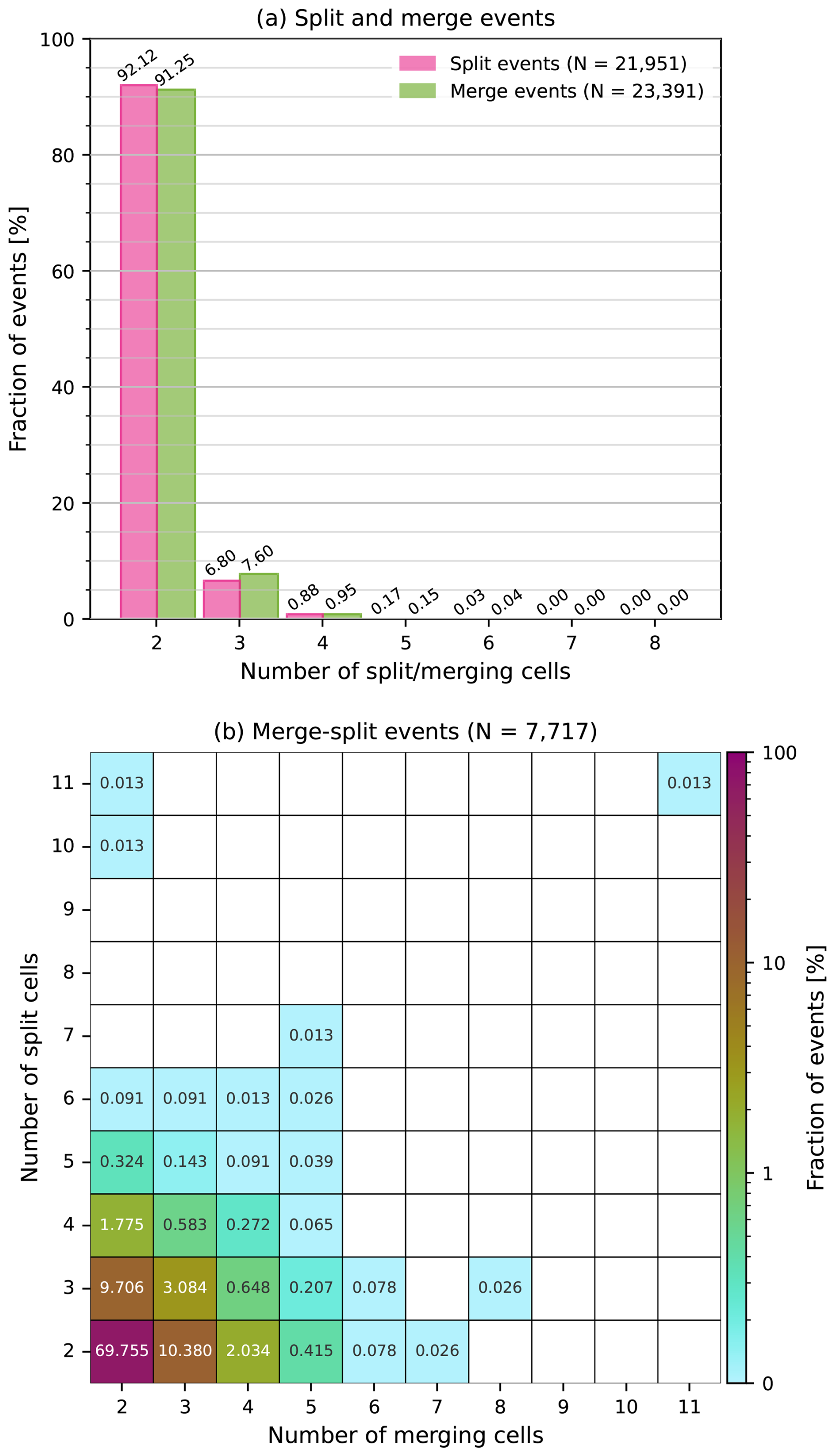
Figure 7 Number of cells participating in (a) split and merge events and (b) merge-split events. In (b) the x-axis shows the number of cells merging and the y-axis the number of cells resulting from the split in the merge-split event.

Figure 8 shows the histograms of cell areas for split, merge, and merge-split events, and for the cells involved in the splits and merges in the events compared to all identified cells. Note that for the cells involved in the splits or merges, the histograms only include the cells that are part of the subgraph of the split or merge event node. The split and merge event cells (Fig. 8a and b) tend to be significantly larger compared to all cells. These event cells are either cells that will split into multiple cells or cells formed by a merge of multiple cells. Because the split or merge event is captured at a random stage of the split or merge process, the event cells can be thought to consist of multiple cells identified as one, which makes them naturally larger than identified isolated cells. However, for the cells involved in split, merge, or merge-split events, the histograms of cell areas are similar compared to all cells, with slightly lower peaks at small areas, indicating that the split or merging cells tend to be only slightly larger than other cells.

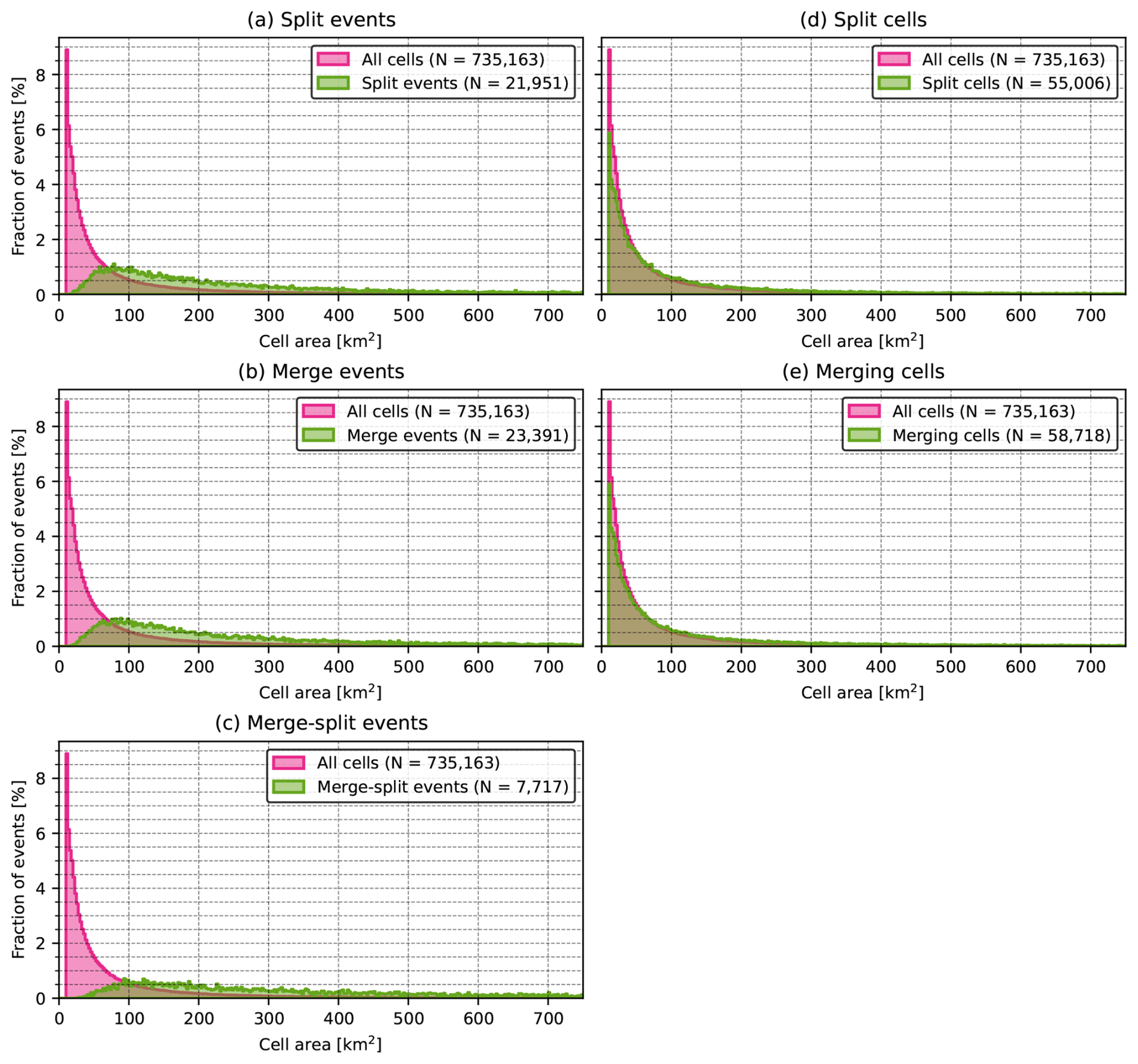
Figure 8 Histograms of cell area in (a) split events, (b) merge events, (c) merge-split events, (d) the cells merging in merge and merge-split events, and (e) split cells in split and merge-split events. The histogram is shown for the cells (a) before splitting in split events and (b) after merging in merge events. In merge-split events (c), the cell is the cell formed by the merge that has not yet split. Note that for the cells involved in the splits (d) or merges (e), the histograms only include the cells that are part of the subgraph of split, merge, or merge-split event.

If selecting the “most representative” cell in a split or merge event based on the cell area, one of the cells should be clearly larger and thus have a greater impact than the other cells. Figure 9 shows the ratio of the smallest cell area to the largest among the cells resulting from the split in split events and the cells merging in merge events. When the largest cell involved is larger than 100 km², the area of the smallest cell is likely less than 30 % of the largest cell's area, and the larger the largest cell, the smaller the ratio of the cell areas. For these split and merge events, the largest cell could be selected as the “most representative” cell likely without much loss of information. However, for events where the largest cell is smaller than 100 km², there is no clearly preferred size of the smallest cell relative to the largest, and selecting the “most representative” cell from cells of similar sizes is more likely to result in information loss in the “most representative” track. Additionally, approximately 40 % of events fall in the category of areas smaller than 100 km², and the number of events decreases in the higher area categories. This is also indicated in Fig. 8d and 8e, where most cells are smaller than 100 km². Thus, in a large portion of split and merge events, the definition of the “most representative” track is questionable when looking at the immediate development of the cells.

Figure 9 The area ratio of smallest to largest participating cell in (a) split and (b) merge events.

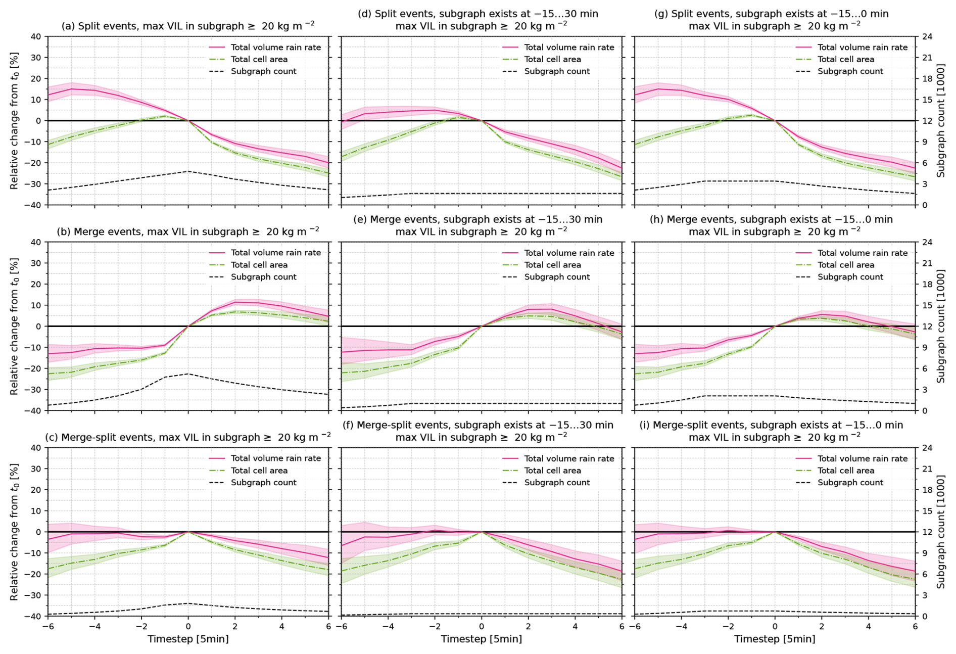
Figure 10 Mean relative change in total cell volume rain rate and total cell area before and after (a, d, g) split, (b, e, h) merge, and (c, f, i) merge-split events. Panels (a)–(c) are calculated over all subgraphs in the dataset where the maximum VIL inside any cell is $\ge \mathrm{20}\mathrm{kg}{\mathrm{m}}^{-\mathrm{2}}$, while (d)–(f) are calculated over subgraphs that exist at least from −15 to 30 min, and (g)–(i) for subgraphs that exist at least from −15 min to t₀. The shaded areas indicate the 95 % confidence intervals of the mean.

4.2 Cell development surrounding splits and merges

Finally, we examine the development of the convective cells related to the events. Figure 10a-c illustrates the mean relative change in total volume rain rate and cell area within the −30 to 30 min window surrounding the event. To emphasize the most severe convective cells, Fig. 10 presents subgraphs where at least one cell has a maximum VIL value greater or equal to 20 kg m⁻². For comparison, the same figure calculated over all subgraphs is shown in Fig. C1.

Split events (Fig. 10a) appear to occur following a decrease in total volume rain rate, but an increase in total cell area. This suggests that splits occur during a decaying stage of cell development, where rainfall diffuses within the cells, resulting in smaller volume rain rates but larger cells. After the split, both the total volume rain rate and cell area decrease sharply. However, a part of the decrease occurring between t₀ and t₁ can be attributed to the area lost between the cells during the split.

Merge events (Fig. 10b), in contrast to split events, seem to occur after a sharp increase in both total volume rain rate and cell area between t₋₁ and t₀. This may be at least partly due to horizontal expansion of the identified cell into the areas between the merging cells. After the merge event, there is some short-lived increase in total volume rain rate and area, but on average, both begin decreasing slowly after 10 to 15 min.

In merge-split events (Fig. 10c), the trends in relative change before the event are similar to merge events and afterwards to split events; however, the rate of increase or decrease is lower. This suggests that, even though the merge-split events might involve more cells than split and merge events, the development is still similar, and separate treatment for merge-split events might not be necessary.

When analyzing cell development in the events, it is important to consider the time window used in subgraph selection, as it can impact the results. As an example, the mean relative change is shown for two other samples: in Fig. 10d–f, the relative change is averaged over subgraphs that exist at least between −15 and +30 min, and in Fig. 10g–i, for subgraphs that exist between −15 min and t₀. This corresponds, for example, to a situation where a forecast model is trained on all samples that exist from −15 to +30 min, but during inference, the model is applied to all subgraphs that exist between −15 min and t₀ (as at inference, it is unknown if the subgraph exists beyond t₀). In this case, the model might, on average, slightly overestimate growth after merge events and underestimate decay after splits. This effect is more clearly observed when examining all events without filtering based on the maximum VIL in Fig. C1.

Note that the existence of the subgraph is not equivalent to the existence of the cell track continuing from the event node: a subgraph existing at a certain time step means that we were able to select the subgraph at that time step, and, conversely, if a subgraph does not exist at some time step, it means that we were not able to select it. This could be either due to the subgraph selection being stopped previously, or because there are no cells in the cell track at that time step (relative to the event node for which the subgraph is selected). Thus, we should be careful when interpreting the results as they apply only to the subgraphs existing at the studied time steps, and conclusions cannot be drawn from the length of the time interval during which a subgraph exists.

5 Conclusions and summary

Cell identification and tracking algorithms are commonly used for analyzing the lifecycle of convective cells and nowcasting their future development based on weather radar data. However, splits and merges in the tracks complicate the use of these algorithms, especially for quantitative analysis of large datasets. To simplify the analysis, a common approach to handle the splits and merges is to define “most representative” tracks. However, in rapidly evolving convective systems, splits and merges of the cells are unavoidable, and ignoring them removes valuable information from the analysis. Previous studies have mainly focused on evolution of the cell tracks over their full life cycles, and not on how to address the splits and merges when analyzing the cell development in short time windows.

The aim of this study was to develop a methodology for quantitative analysis of convective cell development before and after selected events, allowing for the inclusion of splits and merges in the analysis, suitable for analysis across large datasets. In this methodology, cell tracks, created by identifying and tracking convective cells in radar data, are represented as directed graphs. Event nodes, whose development we are interested in, are then selected from the cell tracks. After this, for each event node, a subgraph of predecessor cells that are connected to the event node and successors cells the event node is connected to is selected according to the algorithms presented in the study, aiming to retain the available information in the subgraph at each time step. Once selected, the cell features in the subgraphs are aggregated over each time step to produce a time series.

We demonstrated the methodology by applying it to a dataset of cell tracks identified from operational weather radar products from the Swiss national radar network, using data from May to September over three years. The cell identification and tracking algorithms were applied to study total rainfall and its development in convective cells. To demonstrate the impact of splits and merges on cell development, all split, merge and merge-split cells were selected as the event nodes and subgraphs were constructed for them. We demonstrated the methodology with case studies, and examined through statistical analyses of the split and merge events why, in this dataset, including the splits and merges provides critical information for the analysis of cell development. It was documented that splits and merges occurred in 7.2 % of all identified cells, and they were more frequent in cells with maximum VIL $\ge \mathrm{20.0}\mathrm{kg}{\mathrm{m}}^{-\mathrm{2}}$ (17.9 %) or containing Z_drC features (11.7 %). Commonly used approach of determining the “most representative” cell in a split or merge is not well defined for small cells (<100 km²). In such cases we found no clear preference for a “most representative” cell among the cells involved in the split or merge. In cases where at least one of the cells is larger than 100 km², the other cells tend to be significantly smaller. When looking at the cell development and how it is affected by merges and splits, we found that cell merges were associated with growth in total rainfall and cell area, while cell splits were associated with decrease in total rainfall.

The benefits of the proposed methodology are its versatility and scalability over large datasets. It can be applied to cell tracks obtained through any identification and tracking algorithms, allowing for use in various applications, and it can be applied to quantitatively analyze large datasets. However, even though explicitly including the splits and merges in the analysis can partially mitigate uncertainties caused by inconsistent cell identification and tracking, the results will, as with any cell-based analysis, depend on the cell identification and tracking algorithms used. Furthermore, the time window over which the subgraphs are analyzed impacts the available sample and results, influencing the conclusions drawn. The methodology cannot be applied to study full cell life cycles because the subgraph selection can be stopped even though the cell track would continue; rather, the focus is on cell development within a pre-determined short time window surrounding events of interest.

The proposed methodology can be further developed for more advanced analysis of cell development. While currently cell features in the subgraphs are aggregated into a single time series, they could be analyzed using algorithms specialized for graphs. For example, the past and future parts of the subgraphs can be separate graphs and could be, for example, clustered using graph clustering algorithms (Bunke, 2000; Günter and Bunke, 2002; Bunke et al., 2003) or graph neural networks (e.g. Xia et al., 2025) to match and group similar subgraphs. This would also allow for determining the similarity of two subgraphs, which could be used, for example, in nearest-neighbour or analogue-based nowcasting (Foresti et al., 2015; Shehu and Haberlandt, 2022). However, defining mappings between the subgraphs (Yunwen Xu et al., 2013), for example, to estimate similarity between to subgraphs is not straightforward due to the different sizes of the subgraphs and the lack of shared nodes. Thus, any mappings or definitions of similarity depend on which properties of the subgraphs are relevant for the application and how similarity between two cells is measured.

The proposed methodology can be used in various cell tracking applications. It can be applied, similarly to this study, to produce climatological information on cell development under certain conditions. Additionally, the constructed subgraphs can be expanded to consider also spatial connections between the cells, such as clustering or multiscale cell identification (e.g. Hou and Wang, 2017) to allow for the analysis of larger convective systems. The methodology could also be used to evaluate how well grid-based nowcasting models reproduce the development of convective cells, similarly as in Ritvanen et al. (2025b), while accounting for both true splits and merges in the cell tracks as well as artificial splits and merges caused by blurring in the nowcasts. In addition to cell development, the subgraphs could be used to analyze the severity of cells related to hazards and to create nowcasting models to predict future hazard levels and produce warnings (e.g. Rossi et al., 2012; Tervo et al., 2019). Beyond convective cells, the methodology can be applied also to any dataset that can be represented as spatio-temporal graphs. The methodology presented in this study offers opportunities to significantly advance the knowledge of convective storm development and other systems with complex dynamics.

Appendix A: Convective cell identification and tracking algorithm

The cell identification and tracking algorithms applied in this study are simplified versions of what was applied by Rossi et al. (2012, 2015) and Tervo et al. (2019). The main changes in the algorithms are identifying the cells from vertically integrated liquid fields (VIL) instead of radar reflectivity, and not applying a spatial clustering to the cells.

For cell identification, the VIL field is first pre-processed by transforming the field into binary field using a threshold of 1.0 kg m⁻². To reduce noise in the fields, morphological opening and closing operations with kernel sizes of 3 × 3 km are applied to the fields. After this, the cells are identified by finding closed contours in the resulting binary field. All cells smaller than 10 km² (i.e., 10 pixels) are discarded. The VIL threshold of 1.0 kg m⁻² was selected as it is the lowest value discernable from background values (0.5 kg m⁻²) in the VIL product; in previous studies where cells have been identified from VIL fields thresholds as low as 0.01 kg m⁻² have been used (Hu et al., 2019; Lamer et al., 2023; Tuftedal et al., 2024).

In cell tracking, at each time step first a motion field is determined between the previous time step t₋₁ and current time step t. The motion field is determined from the rainfall field, as that is expected to be more continuous than the VIL field and thus provide motion fields of better quality. The cells existing at time step t₋₁ are then advected to t using the mean velocity inside the cells as the velocity estimate, similarly as in Muñoz et al. (2018). After this, the overlapping area between each advected cell from t₋₁ with each cell at the current time step t is calculated. Any cell pair where the overlapping area is at least 10 % of the minimum of the two cells' area is considered a connection, and the cell at time step t is marked as a child cell of the cell from time step t₋₁, and, vice versa, the cell at time step t₋₁ is marked as the parent cell of the cell at time step t.

Appendix B: Quality control of Z_dr column data used in case studies

The Z_dr column height (Z_drC) fields used in the case studies in Sect. 3 were initially calculated by the algorithm presented by Snyder et al. (2015). For more specific details regarding the implementation, for example, the pre-processing of Z_dr measurements or the environmental zero isotherm used in the calculation, we refer the reader to Aregger et al. (2025).

After the initial Z_drC field, i.e. the maximum height of Z_dr≥1 dB above environmental zero isotherm, is calculated, we apply additional quality control to the field to reduce noise caused by high Z_dr values most likely not related to convection. The requirements for a Z_drC value in a grid point to be accepted are

1. MaxEcho ≥30 dBZ

2. 800 m ≤Z_drC ≤3000 m

3. Z_drC ≤ ETML₂₀

4. Area of Z_drC ≥5 km²

where MaxEcho is the maximum reflectivity in the vertical column in the grid point and ETML₂₀ is the 20 dBZ echo top height above the environmental zero isotherm. The MaxEcho and echo top values are taken from the operational radar products produced by MeteoSwiss, and the environmental zero isotherm is the same as used in the Z_drC calculation.

Compared to the quality filtering applied in Aregger et al. (2025), our filtering is more cautious to account for the lower Z_dr threshold (1 dB vs. 2 dB) and the different definition of the convective cells used in the study. From the quality conditions, the MaxEcho condition (1) follows Aregger et al. (2025). The minimum and maximum height conditions (2) were set to remove Z_drC features most likely not related to updrafts. The echo top condition (3) was similarly used to remove areas where the high Z_dr occurs outside convective storms, e.g., caused by pristine ice crystals. Finally, the condition for the contiguous area of the Z_drC was set to remove spurious features and noise.

When assigning the Z_drC values to the case studies, we assign to each cell all Z_drC areas that the cell overlaps or touches. If a single Z_drC area touches or overlaps with multiple cells, it is assigned to the cell with whom it has the largest overlapping area.

Appendix C: Convective cell development in all split, merge, and merge-split events

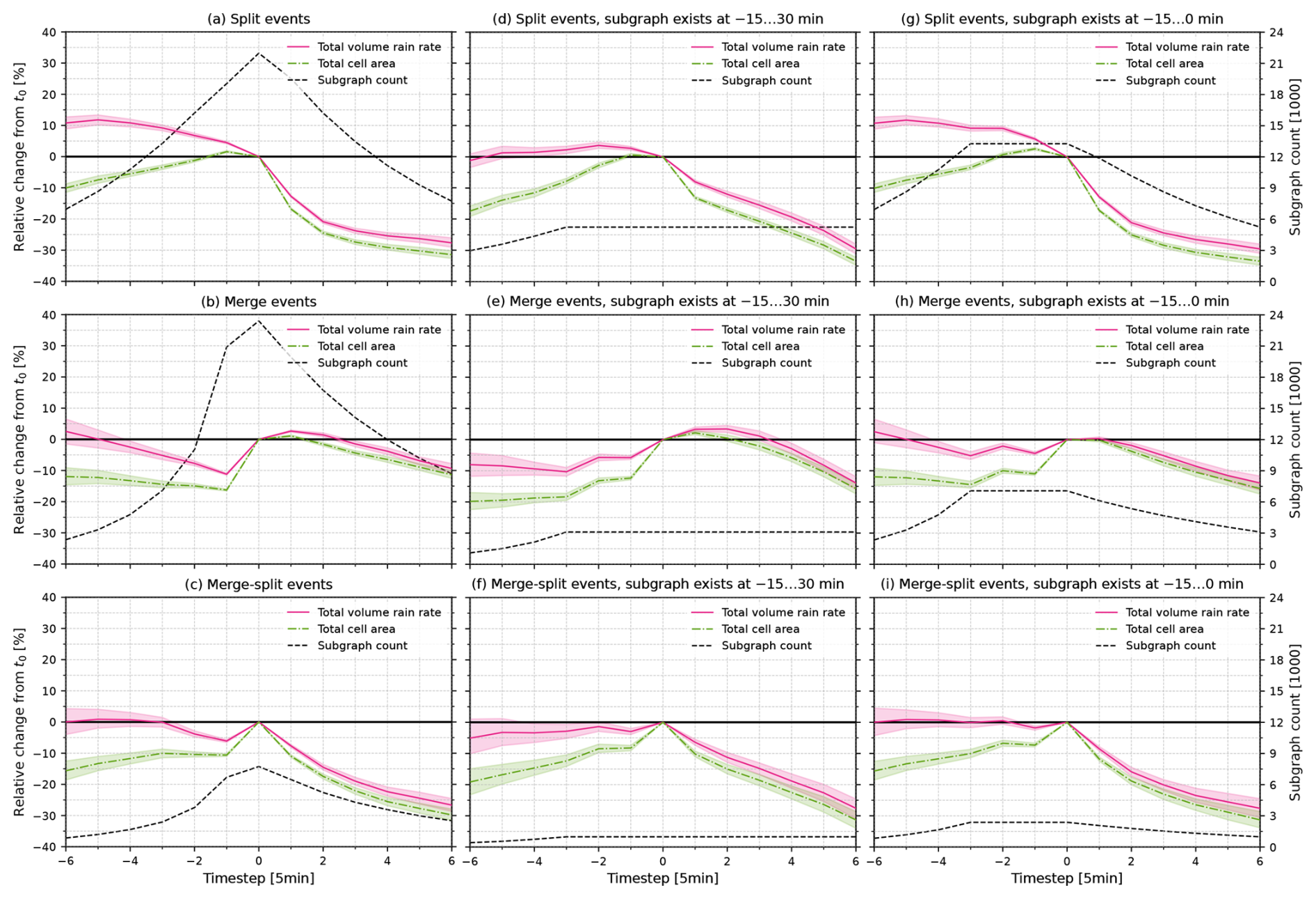
Figure C1 Same as Fig. 10, but calculated without selecting events based on maximum VIL. Mean relative change in total cell volume rain rate and total cell area before and after (a, d, g) split, (b, e, h) merge, and (c, f, i) merge-split events. Panels (a)–(c) are calculated over all subgraphs in the dataset, while (d)–(f) are calculated over subgraphs that exist at least from −15 to 30 min, and (g)–(i) for subgraphs that exist at least from −15 min to t₀. The shaded areas indicate the 95 % confidence intervals of the mean.