Observing long-lived longwave contrail forcing

Contrail microphysical simulations and climate simulations have indicated that contrail cirrus cause a substantial fraction of aviation's climate impact. While the approximations and parameter selections in these simulations have been well-validated over the past 2 decades, the heat trapping of contrails has not been observed using satellite data beyond a few (3–6) hours. This is because contrails lose their linear shape after a few hours, making them difficult to distinguish from natural cirrus clouds. Here we provide satellite-driven analysis of the longwave component of “long-lived” contrail cirrus forcing (i.e. both linear and non-linear contrail cirrus) over North and South America. We aggregate a dataset of GOES-16 estimated outgoing longwave radiation and advected trace density of flight paths, and apply causal inference to discern the effect of contrails while controlling for radiative and cloud confounders. As a means of validation, we also generate synthetic datasets with known ground truth, and confirm that applying the causal inference method is able to recover the synthetic ground truth. Since this method yields an estimate which has some differences from both “instantaneous radiative forcing” (iRF) and “effective radiative forcing” (ERF) estimates which have been reported in the literature so far, we introduce the new term “observational radiative forcing, 12 h” (oRF_H=12). Our analysis estimates the longwave oRF_H=12 from contrails over the Americas averaged 46.9 gigajoules per flight kilometer (95 % CI: 35.2 to 58.6 GJ km⁻¹) during April 2019 to April 2020.

1 Introduction

Condensation trails (contrails) are the ice clouds that form behind jet aircraft as they travel through sufficiently cold and humid air (Schumann, 1996). When ambient atmospheric humidity is supersaturated with respect to ice, contrails can persist for several hours and influence the Earth's energy budget by reflecting incoming solar radiation (during daytime only) and trapping outgoing longwave radiation (at all hours). The net balance of these two effects has been estimated to be warming on average and comparable in magnitude to the warming impact of aviation CO₂ emissions (Lee et al., 2021).

A small number of satellite based studies of contrail radiative forcing have been reported, and can be categorized as following one of three different approaches, each with inherent limitations. The first approach fits a regression to determine the contribution of air traffic to top-of-atmosphere Outgoing Longwave Radiation (OLR) by restricting analysis to an observation region in the North Atlantic, while controlling for confounders by including a regression term for a South Atlantic region that did not contain air traffic (Schumann and Graf, 2013). This spatial restriction limits the potential for the approach to be extended to a globally representative analysis of contrail forcing. The second category of approaches use a linear contrail detection mask (Vázquez-Navarro et al., 2015; Bock and Burkhardt, 2016) or manual bounding of a clear-sky outbreak (Wang et al., 2024a), to demarcate which pixels of the satellite imagery contain exclusively contrails. The reliance on such masks makes it challenging to estimate the overall radiative forcing of contrail cirrus, as masking becomes increasingly error prone in longer-lived contrail cirrus due to the difficulty of distinguishing naturally occurring cirrus apart from contrails which have evolved out of their initial (distinctively linear) morphology. For example, (Vázquez-Navarro et al., 2015) found a central e-folding time of about 2 h for the linear contrails their detector could track. This implies about 95 % of tracked contrails were no longer identifiable as linear contrails after 6 h (either because they have sublimated away or because they have become non-linear), and there does not currently exist a method to separate which cirrus pixels downwind of linear detected contrails are formed from non-linear contrail cirrus versus natural cirrus. The third approach is (Schumann et al., 2021), which leverages the months in 2020 with COVID-19 disruptions in air traffic as a counterfactual, and subtracts off satellite estimates of OLR in those months from the prior year's estimated OLR values to estimate the aviation contribution to OLR. This approach is limited by the uniqueness of this air traffic disruption, and also faces signal/noise ratio issues due to the large natural inter-annual variation in weather conditions (Wilhelm et al., 2021).

Therefore to date, the only technique which could make estimates of the radiative forcing of globally representative samples of “long-lived” contrail cirrus (i.e. including both linear and non-linear contrail cirrus) has been parameterized models, for example climate simulations or microphysical models (Burkhardt and Kärcher, 2011; Chen and Gettelman, 2013; Schumann et al., 2015; Bickel et al., 2020; Teoh et al., 2024). These parameterized models have been developed in recent decades and have used observational data to inform their individual parameter selections, including passive satellite imagers, ground and space lidar, radiosonde, ground camera observations, cloud chamber and in situ ice crystal observations (Freudenthaler et al., 1995; Vázquez-Navarro et al., 2015; Schumann et al., 2017). However, the observational data constraining each individual parameter selection are gathered in specific locations and times which may not be representative of larger populations of contrails, especially considering the high inter-annual variance in contrail prevalence due to year over year meteorological variance (Wilhelm et al., 2021). In particular, microphysical contrails models have been shown to be sensitive to the numerical weather humidity fields they take as input (Teoh et al., 2024; Agarwal et al., 2022), necessitating ongoing research into various correction methods including parametric scaling (Teoh et al., 2022), histogram matching (Platt et al., 2024), and neural networks (Wang et al., 2024b).

Here we introduce a new satellite based methodology for estimating the radiative forcing of long-lived contrail cirrus spanning the diurnal cycle, that does not rely on contrail masking nor on humidity fields from numeric weather data, and has the potential to be applied to globally representative samples of contrails. We pull from the causal inference literature and frame the problem as an observational study estimating an average treatment effect: the treatment is aircraft passage, and the effect is the change in OLR. This framework is well suited for our context: it could be a substantial undertaking to perform a randomized controlled experiment with real aircraft at the scale needed for discerning significance of OLR difference. Causal inference framing also provides a principled statistical structure for isolating a specific causal effect (contrails) from a complex system with numerous confounding variables (meteorology). Causal inference methods have recently been applied to remote sensing problems (Wimberly et al., 2009; Deines et al., 2019; Serra-Burriel et al., 2021; Demarchi et al., 2023; Fons et al., 2023), and the regression fitted by Schumann and Graf (2013) to estimate contrail forcing in the North Atlantic follows a typical causal inference recipe of controlling for confounders, but did not describe their method in causal inference terminology. The main differences between Schumann and Graf (2013) and this work are: (1) we introduce rasterized “advected trace density” as the treatment field, allowing a kilometer scale pixel of a geostationary imager to be the unit of analysis rather than averaging data over millions of square kilometers, (2) we control for confounders using both numerical weather data and geostationary satellite data products, (3) the analyzed domain is spatially larger and more representative of the total population of all contrails, and (4) we investigate our causal inference modeling using synthetic datasets having known ground truth.

2 Methods

2.1 Causal inference regression overview

To estimate the effect of air traffic on OLR, we employ a causal inference framework (Imbens and Rubin, 2015; Pearl, 2009; Holland, 1986; Rubin, 1974). Our approach is designed to isolate the warming impact of contrails from other atmospheric phenomena by modeling the relationship between satellite-observed OLR and air traffic density. This is achieved by explicitly controlling for key environmental confounders, such as the pre-existing weather patterns modeled by ERA5 and the observed cloud state from GOES-16. This helps to disentangle the contrail effect from the influence these conditions may have on flight routing and the formation of natural clouds.

The core of our method is a regression model where the dependent variable is the OLR from the COllocated Irradiance Network (COIN; McCloskey et al., 2023b), a high-resolution flux dataset derived from GOES-16 satellite imagery. As detailed in Sect. 2.2.1, COIN provides OLR estimates at the high spatio-temporal resolution needed to observe contrail effects. This observed OLR is modeled as a linear function of three primary variables: (1) the OLR from the European Centre for Medium-Range Weather Forecasts (ECMWF) ERA5 reanalysis (Hersbach et al., 2018, 2020), (2) the Geostationary Operational Environmental Satellite (GOES-16) L2 cloud phase product, and (3) the advected trace density of air traffic (detailed in Sect. 2.2.2). The mathematical formulation of our model is presented in Eq. (1):

$$\begin{array}{}\text{(1)}& \begin{array}{rl}& \mathbb{E}\left[{\text{OLR}}_{\mathrm{COIN}}|\text{CP},A,{\text{OLR}}_{\mathrm{ERA}\mathrm{5}}\right]\\ & ={\mathit{\alpha }}_{\mathrm{0}}\cdot {\text{OLR}}_{\mathrm{ERA}\mathrm{5}}+\sum _{j=\mathrm{0}}^{\mathrm{4}}{I}_{\left\{\text{CP}=j\right\}}\left({\mathit{\beta }}_j+{\mathit{\gamma }}_{j}A\right).\end{array}\end{array}$$

In this model, OLR_COIN and OLR_ERA5 are the OLR values from the COIN and ERA5 reanalysis, respectively, while A represents the advected trace density of air traffic. The term CP is the GOES-16 cloud phase, categorized as (0) clear sky, (1) liquid water, (2) supercooled liquid water, (3) mixed-phase, or (4) ice. Since contrails are ice clouds, we expect many are included in the CP = 4 category. The model's parameters are interpreted as follows: I_{CP=j} is an indicator function for cloud phase j; β_j represents the baseline OLR adjustment for category j; and γ_j is the conditional effect of advected trace density within that same category. We defer a detailed description of these variables to Sect. 2.2, and discuss the causal model next.

When advected trace density is zero (A = 0), Eq. (1) describes the counterfactual state of the atmosphere with no air traffic; the expected OLR is a function of only ERA5 OLR and the baseline adjustments for each observed cloud phase (β_j): $\mathbb{E}\left[{\text{OLR}}_{\mathrm{COIN}}|\text{CP},A=\mathrm{0},{\text{OLR}}_{\mathrm{ERA}\mathrm{5}}\right]={\mathit{\alpha }}_{\mathrm{0}}\cdot {\text{OLR}}_{\mathrm{ERA}\mathrm{5}}+{\sum }_{j=\mathrm{0}}^{\mathrm{4}}{I}_{\left\{\text{CP}=j\right\}}{\mathit{\beta }}_j$. Our analysis, however, primarily uses the fitted γ_j coefficients to estimate the effect of a small increase in advected trace density given any underlying advected trace density baseline A=a. This allows us to quantify the radiative impact of additional flights while controlling for existing atmospheric conditions.

Our statistical counterfactual is constructed by using the ERA5 reanalysis and GOES-16 cloud observations to control for confounding weather conditions. By incorporating ERA5 OLR as an independent variable, we control for the vast majority of natural atmospheric processes that influence OLR. Since the ERA5 model parameterizes clouds based on the thermodynamic state of the atmosphere and does not assimilate all-sky satellite radiances, it does not explicitly account for contrail formation (Hersbach et al., 2020) and thus serves as a baseline for what the OLR would have been in the absence of contrails. Consequently, the discrepancies between the COIN and ERA5 OLR estimates can be attributed to factors not captured in the ERA5 reanalysis, including the radiative forcing from contrails. This type of use of ERA5 as a counterfactual for analyzing radiative impacts has been applied in recent studies on aerosol–cloud interactions (Chen et al., 2022; Jia et al., 2024). Figure 1 shows the residuals from estimating the model $\mathbb{E}\left[{\text{OLR}}_{\mathrm{COIN}}|{\text{OLR}}_{\mathrm{ERA}\mathrm{5}}\right]={\mathit{\lambda }}_{\mathrm{0}}+{\mathit{\lambda }}_{\mathrm{1}}{\text{OLR}}_{\mathrm{ERA}\mathrm{5}}$; linear contrails and the contrail cirrus they evolve into are clearly visible in the residual imagery, demonstrating the presence of the contrail signal in the data.

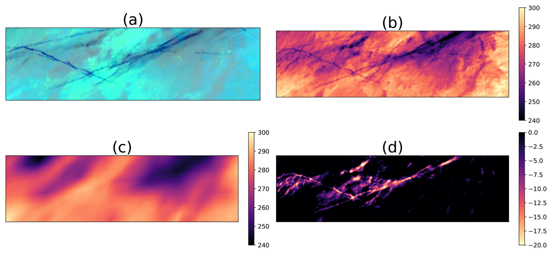
Figure 1 A contrail outbreak scene at 18 July 2019 14:20 UTC, over the southwestern United States. The GOES-16 ABI Ash longwave color scheme in panel (a) highlights the contrails as dark blue linear objects. In panel (b) the GOES-16 based COIN OLR field (in W m⁻²) also shows the contrails trapping thermal radiation, but contrails cannot be seen in panel (c) ERA5 OLR because ERA5 does not model nor assimilate contrails. The panel (d) OLR Residual image is generated by using ordinary least squares to predict COIN OLR as a function of ERA5 OLR and plotting the linear fit residuals; the bright, linear, and web-like features highlight young and aged contrail cirrus that are captured by the satellite observations but not present in the ERA5 model, demonstrating the presence of the contrail signal in the data. Note panel (d) clips the OLR residual to only show negative residuals, for visual clarity; the quantitative analyses – Eqs. (1), (2) and (3) – use all values of their respective variables.

A key challenge, however, is that ERA5's representation of even natural clouds is not perfect. Errors in the model's prediction of cloud location, phase (e.g. ice vs. water), or optical properties can also create differences between the observed COIN OLR and the predicted ERA5 OLR. This is a source of confounding, as air traffic often occurs in the same upper-tropospheric regions that are prone to natural cirrus formation. Without further controls, the model might wrongly attribute the radiative effect of a natural cirrus cloud (that was simply missed or misrepresented by ERA5) to the presence of air traffic.

To address this, we include the GOES-16 L2 cloud phase product as an independent variable. This provides direct satellite observations of the actual cloud state (e.g., clear sky, ice cloud, water cloud) in each pixel. By including this variable, we allow the model to account for the systematic differences between COIN and ERA5 OLR that are due to the presence of different types of clouds independent of air traffic. For example, the model allows us to estimate the average OLR discrepancy that occurs when GOES-16 observes an ice cloud that ERA5 did not estimate to be there. Explicitly controlling for the observed cloud state allows the model to more accurately isolate the remaining effect attributable to the advected trace density. This step allows Eq. (1) to better distinguish between OLR anomalies caused by ERA5 inaccurately estimating cloud properties (e.g. by missplacing a cirrus cloud – represented by β₄) apart from an anomaly caused by a contrail that ERA5 does not estimate to exist there at all (represented by γ₄). The resulting coefficient, γ₄, therefore represents the average conditional effect of increasing advected trace density on OLR for all pixels classified as ice clouds (CP = 4), a group which contains both natural cirrus and contrails. It can be interpreted as the mean effect of a contrail on top of any ice cloud scene.

The model attributes the difference between COIN and ERA5 OLR to the cloud phase and advected trace density. Through careful normalization of the advected trace density units, the fitted slope of this regression directly quantifies the average contrail effect on OLR per kilometer of flight, as illustrated in Fig. 3.

The coefficients γ_j from Eq. (1) represent the change in COIN OLR per unit of advected trace density for each cloud phase. To find the overall average effect, we calculate the Average Treatment Effect (ATE) by weighting each coefficient by the probability of that cloud phase occurring in the dataset. To give some intuition to this, consider an increase of advected trace density A of δ for supercooled liquid water (cloud phase category 2) pixels with same OLR_ERA5 baseline is: $\mathbb{E}\left[{\text{OLR}}_{\mathrm{COIN}}|\text{CP}=\mathrm{2},A=a+\mathit{\delta },{\text{OLR}}_{\mathrm{ERA}\mathrm{5}}\right]-\mathbb{E}\left[{\text{OLR}}_{\mathrm{COIN}}|\text{CP}=\mathrm{2},A=a,{\text{OLR}}_{\mathrm{ERA}\mathrm{5}}\right]=\mathit{\delta }{\mathit{\gamma }}_{\mathrm{2}}$. Note that, according to our assumptions, we compare sets of pixels that are identical except for advected trace density, and we attribute the change in OLR_COIN to advected trace density. Therefore, we can use Eq. (1) to estimate the average treatment effect (ATE) of an increase in advected trace density on OLR_COIN by integrating out the ERA5 OLR baseline which yields:

$$\begin{array}{}\text{(2)}& \begin{array}{rl}\text{ATE}& ={\displaystyle \frac{\mathrm{1}}{\mathit{\delta }}}(\mathbb{E}\left[{\text{OLR}}_{\mathrm{COIN}}|A=a+\mathit{\delta }\right]-\mathbb{E}\left[{\text{OLR}}_{\mathrm{COIN}}|A=a\right])\\ & =\sum _{j=\mathrm{0}}^{\mathrm{4}}{\mathit{\gamma }}_{j}P(\text{CP}=j),\end{array}\end{array}$$

where δ is the amount of change in advected trace density, P(CP=j) is the probability that a GOES-16 pixel will have cloud phase category j, and $\mathbb{E}\left[{\text{OLR}}_{\mathrm{COIN}}|A=a\right]$ is the expected OLR_COIN conditional on advected trace density, in which OLR_ERA5 and cloud phase have been integrated out.

This equation defines the Average Treatment Effect (ATE) as the average change in OLR_COIN per unit increase (δ) in advected trace density (A). The difference in expectations on the left represents this definition, where the integration is marginalized over the population distributions of all other covariates (OLR_ERA5 and cloud phase). Due to the linear structure of our model, this simplifies to the expression on the right. This final expression is a weighted average of the conditional effects, where γ_j is the specific effect of advected trace density on OLR_COIN when a pixel is in cloud phase j, and P(CP=j) is the area-weighted marginal probability of a pixel belonging to that cloud phase category. This weighting ensures that larger pixels away from the satellite's nadir contribute proportionally to the final estimate.

Analysis results are based on 183 d of data from April 2019–April 2020 (every other day), in the region seen in Fig. 6 which includes much of both North and South America.

2.2 Data fields used in causal regressions

For an overall view of the dataset generation workflow, see Fig. 2.

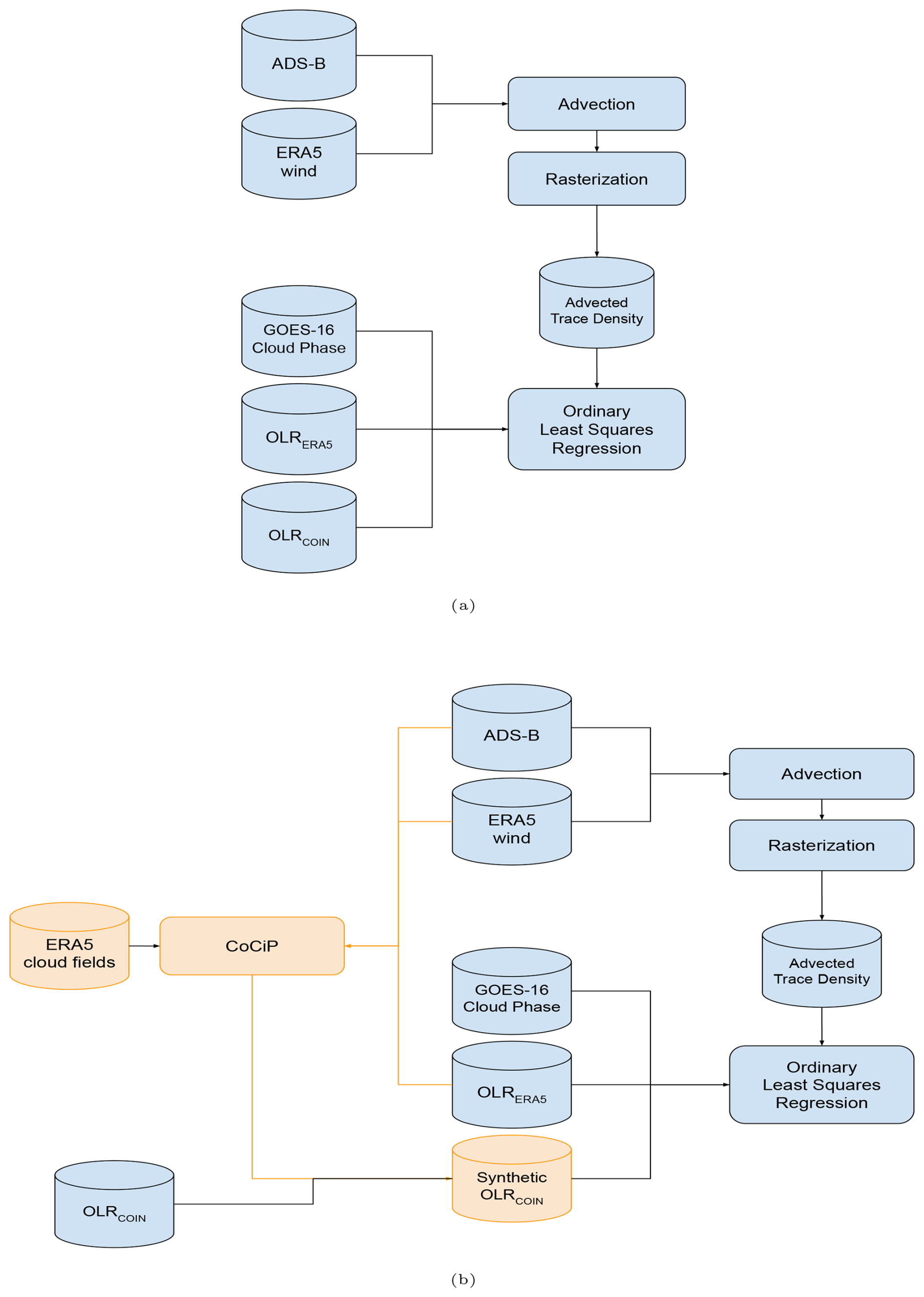
Figure 2 Workflow diagram of dataset generation process for (a) analyzing the real contrail longwave forcing over the Americas and for (b) validating the causal inference method using synthetic known ground truth generated by CoCiP. Items in orange are only found in the synthetic testbed workflow and are not used in the real contrail forcing analysis reported over the Americas.

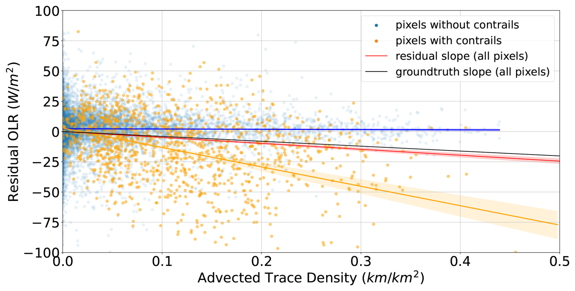
Figure 3 Relationship between advected trace density (x axis) and the ordinary least squares residuals of COIN OLR as a function of ERA5 OLR (y axis), on a sample of synthetic data with known ground truth (see Sect. 2.5 for further details). The plot shows how the regressed difference between ERA5 and COIN quantifies the average contrail effect on OLR. Colors code whether residuals come from contrail pixels (orange) or non-contrail pixels (blue). Fitted lines between flight density and residuals illustrate how the contrail effect is estimated separately when using contrail-only pixels (contrail effect) vs non-contrail (no effect) or all pixels (advected trace density effect from contrails).

Prior to performing regressions, data fields are reprojected (if necessary) onto a common spatial grid of pixels: the grid used by GOES-16 Advances Baseline Imager (ABI) longwave bands, which has shape 5424 × 5424 covering the western hemisphere as viewed from geostationary orbit at longitude −75 °. Hereafter this will be referred to as the “ABI pixel grid”. The pixels are nominally 2 km per side, but increase in size with increasing viewing angle away from nadir. Where calculations require multiplying by pixel area, we estimate the pixel area in m² by calculating the great circle distance between adjacent pixel centers and applying the trigonometric formulae for parallelogram area based on these side lengths. For visualization and area formula see Appendix B.

2.2.1 COllocated Irradiance Network (COIN) flux

The COIN model was developed as a method of estimating broadband irradiance (flux) from GOES-16 ABI narrowband radiances, in order to have the spatio-temporal resolution needed (nominally 2 km spatial resolution with a 10 min refresh rate) to observe contrail effect on the Earth's top-of-atmosphere upwelling irradiance (McCloskey et al., 2023b). Briefly, COIN is a neural network model trained to make pixel-wise estimates of flux (OLR and RSR in units of W m⁻²) on a dataset of GOES-16 ABI input radiances collocated with Cloud and Earth's Radiant Energy System (CERES) Level2 SSF (Wielicki et al., 1996) and Level3 SYN1deg flux labels (Doelling et al., 2016). The COIN model is a fully connected neural network operating pixelwise on all bands of GOES-16 Level 1b radiances as input, along with 5 auxiliary inputs: the latitude, the longitude, the solar zenith angle, the solar azimuth angle, and the day of the year. The COIN model error was minimized using mean squared error loss against the CERES L2 and L3 OLR and RSR flux labels by backpropagating gradients through the CERES sensor's point spread function. Here we use the COIN estimates of OLR which were released alongside (McCloskey et al., 2023a) and available at https://console.cloud.google.com/storage/browser/upwelling_irradiance/ceres_goes/ (last access: 30 June 2025). See Sect. 2.5 (specifically the “Measurement bias” variation) and Sect. 4.2 for discussion of the potential impact of bias in COIN estimates of OLR on estimates of contrail longwave forcing.

2.2.2 Advected trace density

We introduce the concept of advected trace density which represents the expected value of contrail length (in kilometers) inside an area, if every flight path had created a persistent contrail.

Advected trace density is an extension of the concept of advecting Automatic Dependent Surveillance-Broadcast (ADS-B) flight trajectory waypoints, which are then used to derive collocation datasets with satellite sensor data (Duda et al., 2004; Tesche et al., 2016; Geraedts et al., 2024; Sarna et al., 2025); the name “advected trace” was introduced in Chevallier et al. (2023). We begin by advecting flight waypoints provided in ADS-B data licensed from https://www.flightaware.com/ (last access: 30 June 2025) and Aireon, following Geraedts et al. (2024). Flight waypoints are advected using ERA5 wind data with a Runge Kutta 3D method, and additionally sediment downwards using the terminal velocity of an estimated ice crystal size average. We advect each flight waypoint for 12 h.

We extend the advection to model the uncertainty in wind error as a Gaussian whose standard deviation grows linearly over time. In particular, as shown in Fig. 4 we found the error of the ERA5 u and v components of wind grow at 12.4 km h⁻¹, when compared against Mode-S computed wind speeds licensed from https://www.flightaware.com/. We also then normalize the advected trace density field, so that when we rasterize it into the ABI pixel grid, it has units of flight length divided by pixel area: km km⁻². An example of its rasterization can be seen in Fig. 5.

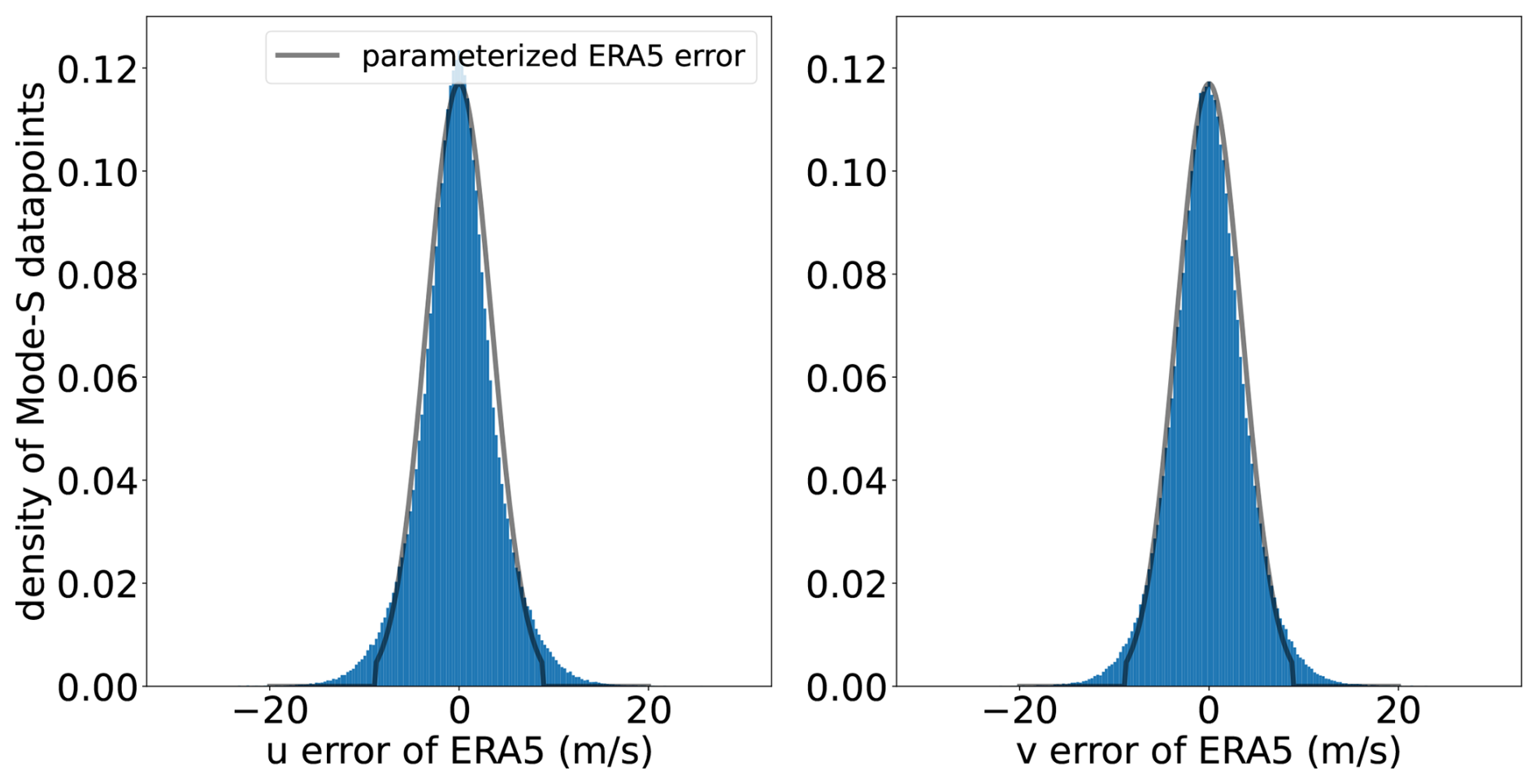
Figure 4 Distribution of ERA5 wind errors. The histograms show the difference between ERA5 u- and v-component winds and those calculated from aircraft Mode-S data. A Gaussian fit (black line) is used to model the wind error uncertainty, which grows at an estimated 12.4 km h⁻¹ and is incorporated into the advected trace density calculation.

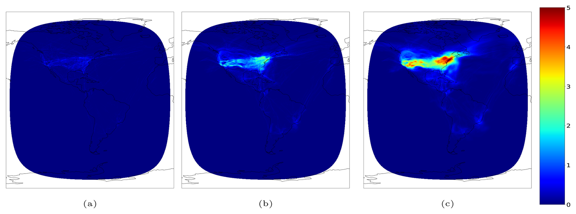
Figure 5 An example of the rasterized advected trace density field (in units of flight kilometer per square kilometer, km km⁻²) from 14 May 2019 at 01:00:00 UTC. Panel (a) shows the density advected for up to 1 h (A_H=0), (b) for up to 6 h (A_H=5) and (c) up to 12 h (A_H=11).

In its simplest form, advected trace density is a 2-dimensional spatial field (“x” and “y” pixel coordinates) on the ABI pixel grid, that also varies with time. To analyze the effect of contrail age, we define D_h as the trace density that has been advecting for h hours (rounding down partial hours), $h\in \left\{\mathrm{0},\mathrm{\dots },\mathrm{11}\right\}$. With these, we define a set of average cumulative advected trace density variables, A_H = $\frac{\mathrm{1}}{H+\mathrm{1}}{\sum }_{h\le H}{D}_h$, for $H=\mathrm{0},\mathrm{\dots },\mathrm{11}$. Each variable A_H represents the average advected trace density from all flight paths with an advection age of less than H+1 hours. For example, A₀ = D₀ includes the density from flight traces advected for less than 1 h, A₁ = $\frac{\mathrm{1}}{\mathrm{2}}(D_{\mathrm{0}}+D_{\mathrm{1}})$ includes the density from all advected traces younger than 2 h, etc. This formulation allows us to fit a separate regression model for each cumulative age H, as shown in Eq. (3), in order to estimate the total longwave forcing as a function of advection duration.

$$\begin{array}{}\text{(3)}& \begin{array}{rl}& E\left[{\text{OLR}}_{\mathrm{COIN}}|\text{CP},A_H,{\text{OLR}}_{\mathrm{ERA}\mathrm{5}}\right]\\ & ={\mathit{\alpha }}_{\mathrm{0}\mathrm{H}}\cdot {\text{OLR}}_{\mathrm{ERA}\mathrm{5}}+\sum _{j=\mathrm{0}}^{\mathrm{4}}{I}_{\left\{\mathrm{CP}=j\right\}}\left({\mathit{\beta }}_{jH}+{\mathit{\gamma }}_{jH}{A}_H\right),\end{array}\end{array}$$

Note that we fit Eq. (3) 12 separate times, one for each cumulative age: $H=\mathrm{0},\mathrm{\dots },\mathrm{11}$. We do this to avoid estimating coefficients for each $D_{\mathrm{0}},\mathrm{\dots },D_{\mathrm{11}}$ because individual hourly advected trace density variables are highly correlated to each other. To mitigate spatio-temporal edge effects from advection in the causal regression, we load ADS-B waypoints from a larger bounding loop (Fig. 6, “Flights loading region”) than we sample from when fitting Eq. (1) (Fig. 6, “Analysis region”). For each of the 183 d in the analysis, we load (and perform 12 h advections) for ADS-B waypoints from 36 h windows, and then only sample from the final 24 h of each 36 h window when estimating the causal model.

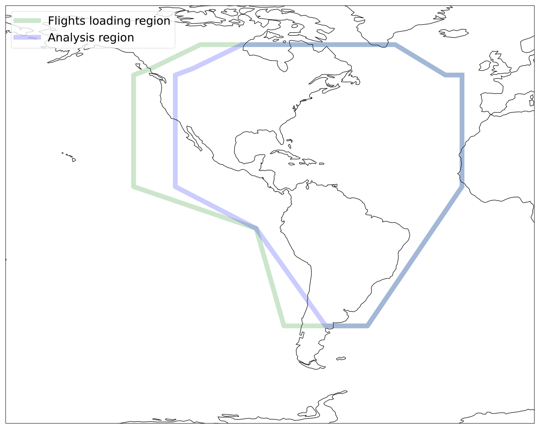
Figure 6 Geographic domain of the study. ADS-B flight data was loaded from the larger (green) outer polygon to create the advected trace density field. To mitigate advection related edge effects, the causal regression was then performed on pixels sampled from within the inner blue polygon which is smaller in places that have prevailing flight level winds in a certain direction.

2.2.3 ERA5 OLR

Prior to performing the estimation of the causal model parameters in Eq. (1), we must convert the ECMWF ERA5 OLR field (which has units J m⁻² accumulated over the hour timestep of the weather model, on a 0.25° latitude/longitude grid) into a form that allows pixel-wise analysis with the other data fields in the model. To accomplish this, we first divide the hourly-accumulated ERA5 OLR by 3600 s to yield flux in units of W m⁻², and then apply a reprojection using linear interpolation in the spatial dimension onto the ABI pixel grid, applying parallax correction for the top of atmosphere flux using a nominal top-of-atmosphere altitude of 20 km. Temporally, we apply nearest-neighbor interpolation.

2.2.4 GOES-16 L2 Cloud Top Phase product

The GOES-16 ABI Cloud Top Phase algorithm (GOES-R Algorithm Working Group and GOES-R Series Program, 2023; Heidinger et al., 2020) determines the top-altitude cloud phase by analyzing infrared radiances (specifically 7.4, 8.5, 11, and 12 µm channels). It converts these radiances into effective cloud emissivities and “beta-ratios” (ratios of effective absorption optical depths), and applies a decision tree based on threshold tests to classify cloud tops into categories of warm liquid water, supercooled liquid water, mixed phase, and ice.

2.3 Computational expense

As a rough estimate of the computational expense of generating all data fields detailed in Sect. 2.2, a breakdown of the number of CPU core-hours needed to generate 1 d of causal regression input data aligned on the ABI pixel grid (144 scantimes) for each step is as follows:

• -

  COIN flux: 0 core-hours (already available)

• -

  GOES-16 Cloud Top Phase: 0 core-hours (already available)

• -

  CoCiP: ≈ 650 core-hours (used only in synthetic tests or comparisons to causal inference regressions)

• -

  Advected trace density:

  • -

    ≈ 50 000 core-hours if using a dense rasterization technique where all ABI pixel grid pixels are rasterized OR

  • -

    ≈ 500 core-hours if using a sparse rasterization technique where only pixels actually randomly sampled for causal inference regression are rasterized.

• -

  ERA5 OLR: ≈ 80 core-hours for reprojection into the ABI pixel grid.

• -

  Collation of all fields for 1.5 × 10⁹ sampled pixels: ≈ 75 core-hours.

2.4 Block Bootstrap uncertainty quantification

To estimate confidence intervals of our central estimate of contrail longwave RF, we apply bias-corrected block bootstrap (Künsch, 1989) where a block consists of pixels within the same day. This helps maintain the flight traffic and synoptic weather covariance structure of the data. Specifically, we first sample 183 d with replacement, and then proceed to sample pixels within each sampled day to sample a total of 500 000 pixels, filtering to maintain a ratio of at most 1 % of pixels having A_H = 0 to avoid biasing the OLS fits with an overwhelming number of data points which were not exposed to the advected trace density treatment. We then estimate the model coefficients and compute the corresponding value in units of gigajoules per flight kilometer. This sampling and estimation process is repeated 1000 times. We show the central estimate derived from a sample of 3 million pixels. To derive the 95 % confidence interval, we overcome the finite-sample bias introduced by the block bootstrap (Lahiri, 2003a, b) by applying a correction defined as the difference between the central estimate and the average of the 1000 bootstrap estimates. This procedure re-centers the distribution on the more accurate central estimate (Efron, 1987), and our final 95 % confidence interval is derived from the 2.5th and 97.5th percentiles of this bias-corrected distribution.

2.5 Synthetic dataset validations

To validate and probe this method, we generate a few synthetic versions of this type of dataset using the pycontrails v52.2 implementation (Shapiro et al., 2024) of CoCiP (Schumann, 2012), where we are able to record the synthetic known ground truth value of the longwave forcing per flight kilometer to confirm the regression method can recover it from being embedded in situ among natural confounders and error covariances. We created the synthetic datasets exclusively in the southern hemisphere, where flight density is much lower than in the northern hemisphere, to avoid accidentally creating unrealistic modeling difficulties by aligning synthetic contrails with real contrails. The synthetic dataset is composed of the same data fields as the real dataset:

1. A synthetic advected trace density field is rasterized, by loading real ADS-B waypoints for flights traversing the Conterminous United States (CONUS), flipping their latitudes into the southern hemisphere (multiplying by −1), and then applying the same 12 h advection and rasterization as described in Sect. 2.2.2; advections were performed using the ERA5 wind data from their latitude-flipped (southern hemisphere) waypoint locations.

2. A synthetic COIN OLR field is rasterized, starting from the real COIN field provided for the southern hemisphere by McCloskey et al. (2023a). Then, taking the same latitude-flipped ADS-B waypoints used above, we estimate the contrail longwave forcing using CoCiP; in all pixels where CoCiP estimates that (based on the unmodified southern hemisphere ERA5 weather fields) there would be nonzero longwave forcing we subtract it from the original COIN OLR at that location on the ABI pixel grid. The details for rasterizing the CoCiP forcing follow the rasterization of CoCiP contrail opacity in Sarna et al. (2025), with the exception that instead of rasterizing a thresholded opacity mask here we are rasterizing the CoCiP “rf_lw” property (or in one variant below, the flux as a parameterization of the “tau” optical depth property). CoCiP executions did not use any regional/temporal subsampling and were performed using linear interpolation of meteorological inputs, a 30 s timestep, and corrected ERA5 humidity using the pycontrails “histogram_matching” option described in Platt et al. (2024). An example of the synthetic COIN OLR field (“Linear overlap” variation) can be seen in Fig. 7c.

3. A synthetic GOES-16 L2 Cloud Top Phase field is used, which is only a slightly modified version of the real data: pixels where CoCiP rf_lw is nonzero have a 74 % random chance of becoming set to Cloud Phase 4 (ice cloud), to account for inaccuracies reported in Jiménez (2020).

4. An unmodified ERA5 OLR field (the real field from the southern hemisphere, reprojected as in Sect. 2.2.3) is used in the estimation of Eq. (1).

We generate four variations of such synthetic datasets:

• “Linear overlap”: in this variation, CoCiP estimates of rf_lw are summed linearly in rasterized pixels. (This is currently the default operating mode of pycontrails and all CoCiP studies in the literature we are aware of to date.)

• “Sublinear overlap”: in this variation, the CoCiP estimates of tau (contrail optical depth) from different contrails in the same pixel are summed in log space, creating an “effective tau” which is then converted to rf_lw via an approximation detailed in Appendix A. This variation investigates whether estimating Eq. (1) as a linear function introduces estimation error when the effect on OLR with increasing advected trace density is likely to be somewhat sublinear in reality.

• “Measurement bias”: in this variation, each of a “Linear overlap” and “Sublinear overlap” synthetic dataset are further modified to introduce simulated measurement bias of the type that was noted as occurring in the COIN estimates relative to CERES flux labels in Fig. 4 of McCloskey et al. (2023b). This variation investigates whether the estimation of Eq. (1) is robust to this type of systematic bias.

• “Null”: in this variation, we fit Eq. (1) using a latitude-flipped synthetic advected trace density field as usual, but coupled with an unmodified real COIN OLR field from the southern hemisphere which did not have aircraft in those places making contrails. That is, in this variant the ground truth contrail longwave forcing caused by this advected trace density is zero, but typical levels of discrepancy between ERA5 OLR and COIN OLR from other causes exist in the dataset and could potentially bias the regression estimate to return a non-zero answer; using this variant, we confirm that the Eq. (1) regression correctly returns an estimate of zero contrail forcing.

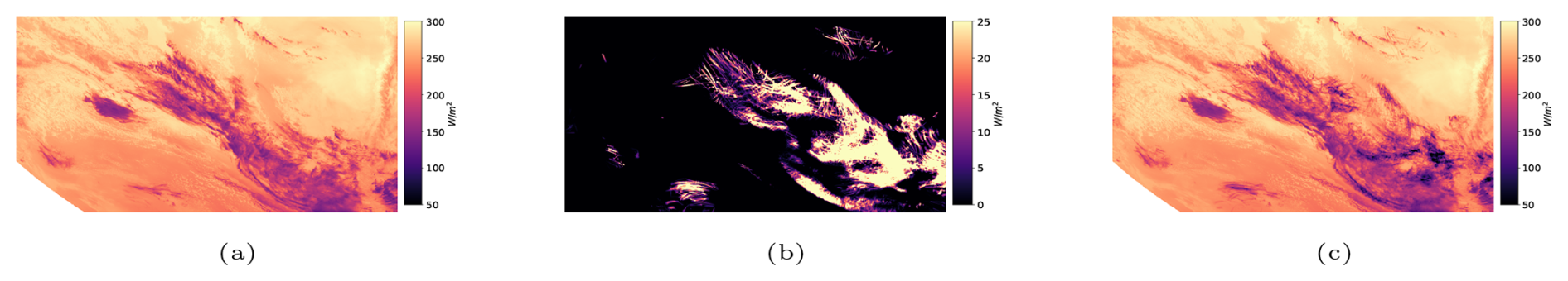
Figure 7 Example of a synthetic COIN OLR field used for model validation. Panel (a) shows the observed OLR field in the southern hemisphere. The observed flight tracks from the northern hemisphere were latitude-flipped and used to generate contrails according to the CoCiP model as shown in panel (b). The longwave forcing from these synthetic contrails was then subtracted from the observed OLR field in the southern hemisphere, creating a dataset with a known ground truth forcing as shown in panel (c).

3 Results

3.1 Insight from synthetic datasets

An important observation from regressing against the synthetic OLR datasets is that many of the discrepancies between COIN OLR and ERA5 OLR are of a similar (or larger) magnitude than the effect size of contrail forcing that has been estimated in the literature to date. Because of this – and because air traffic levels are high enough that large portions of CONUS have nonzero advected trace density at most hours of the day – it is likely that at any given time there exists co-occurring advected trace density and COIN-ERA5 discrepancy in the same pixels not actually caused by contrails. In this situation, a small sample of such pixels could return a non-zero radiative forcing estimate which is entirely caused by such spurious correlations. For our purpose of making a low bias estimate of average contrail longwave forcing, we must draw a large sample of independent observations so these spurious correlations can cancel each other out during the regression. Crucially, we note that spatio-temporally adjacent pixels are not independent observations: to usefully increase the sample size pixels must be sampled from a large number of independent synoptic weather patterns, and we achieve this by sampling from different days. See Fig. 8 for details on estimate bias as a function of number of days sampled and number of pixels sampled; we observe that only a few hundred thousand pixels are necessary for a low bias estimate of the synthetic ground truth forcing, as long as they are sampled from a few dozen different days.

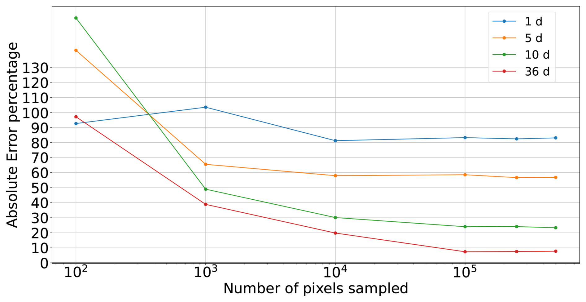
Figure 8 Convergence of the longwave forcing estimate as a function of the number of pixels sampled in the “Linear overlap” synthetic dataset test. As the number of independent days sampled increases the error decreases, but sampling more than a few 100 000 pixels does not seem to improve the error.

As seen in Fig. 9, we find that with a sufficiently sized (and sufficiently independent) input sample, the regression method provides a low bias estimate for all of the “Linear overlap”, “Sublinear overlap” and “Measurement bias” tests, as well as correctly returning close to zero contrail forcing in the “Null” test.

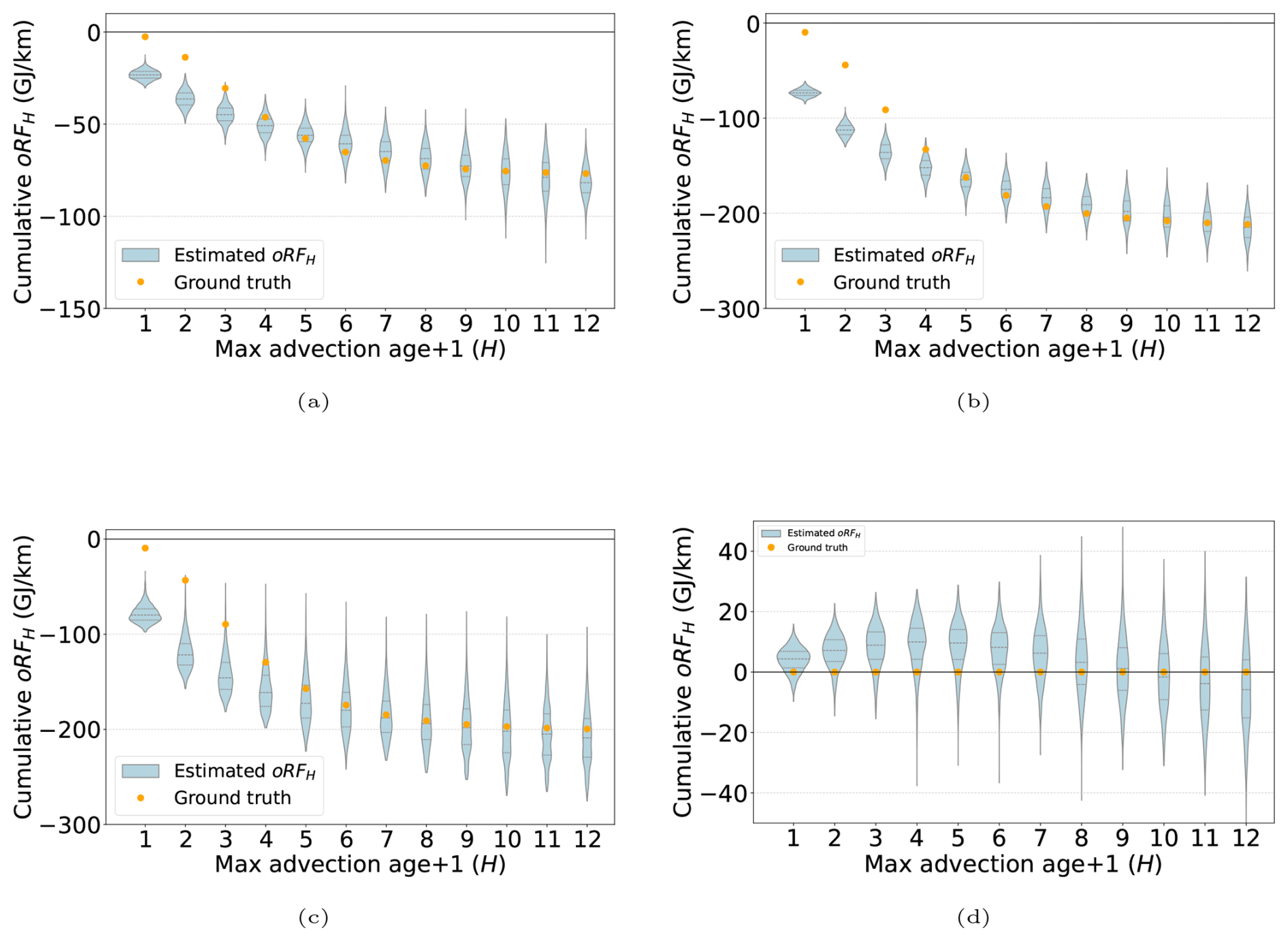
Figure 9 Validation of the causal inference method on synthetic datasets. The plots show the estimated contrail longwave forcing (blue violins) versus the known synthetic ground truth longwave forcing (orange dots) as a function of advected trace density age using Eq. (3). Each panel shows the distribution of the estimated longwave forcing (oRF_H) from the twelve separate OLS fits, one violin per fit of a cumulative age $H\in \mathit{\{}\mathrm{0},\mathrm{\dots },\mathrm{11}\mathit{\}}$. The model successfully recovers the known ground truth in the (a) “Linear Overlap”, (b) “Sublinear Overlap”, and (c) “Measurement Bias” tests, and (d) correctly returns a near-zero longwave forcing for the “Null” test, where no contrails were present.

To further validate that our forcing estimate in the Americas is not a product of spurious correlation, we also performed a permutation test where the advected trace density values were randomly shuffled among all pixels. By breaking any real causal link between air traffic and OLR, we expect the model to find no significant effect. Specifically, the fitted interaction coefficients, which measure the impact of advected trace density for each cloud phase, should be statistically indistinguishable from zero: ${\widehat{\mathit{\gamma }}}_j$ = 0. As expected, this test correctly returned a near-zero longwave forcing estimate of −0.01 GJ km⁻¹ (95 % CI: −0.47 to 0.46 GJ km⁻¹), providing strong evidence that our longwave central estimate is statistically significant and not due to chance.

We also use the synthetic dataset to assess the calibration of our bootstrap confidence intervals, and indeed saw that on the “Linear overlap” dataset the nominal 95 % confidence intervals correctly captured the known ground truth in 95 % of trials. This confirmed that our chosen day-block bootstrap method is well-calibrated.

3.2 Central estimate of contrail longwave forcing in the Americas

In the spatial domain seen in Fig. 6b, during April 2019–April 2020, contrails averaged 46.9 GJ of longwave oRF_H=12 per flight kilometer. The 95th percentile confidence interval is 35.2 to 58.6 GJ km⁻¹ (p < 0.001). We also performed a permutation test, randomly permuting the advected trace density among pixels in the dataset but leaving the other fields unmodified, followed by fitting Eq. (1) on the permuted version of the dataset. If this test returned a nonzero answer, it could indicate that our central estimate may not be statistically significant. However, the permuted regression correctly returns very close to zero longwave forcing: estimate: −0.01 (95 % CI: −0.47 to 0.46) GJ km⁻¹.

To place our observational result in the context of an established contrail model, we also calculated the instantaneous radiative forcing (iRF) for the same set of flights using CoCiP (Shapiro et al., 2024; Schumann, 2012). Running CoCiP over the same time period (April 2019–April 2020) and geographic region shown in Fig. 6 yielded a total longwave iRF estimate of 60.7 GJ km⁻¹. Note that as is currently common in the literature we executed CoCiP in “offline” mode where it is not coupled to the simulated atmosphere it uses as input (in this case ERA5), so it does not include any atmospheric feedback effects which may be captured by our observational method.

The results from the fitted Eq. (1) are presented in Table 1. The primary finding is the Average Treatment Effect (ATE), which shows that an increase in advected trace density has a statistically significant warming effect, changing OLR by an average of −13.036 $\frac{\mathrm{W}{\mathrm{m}}^{-\mathrm{2}}}{\mathrm{km}{\mathrm{km}}^{-\mathrm{2}}}$ (95 % CI $[-\mathrm{16.281},-\mathrm{9.79}]$). The units $\frac{\mathrm{W}{\mathrm{m}}^{-\mathrm{2}}}{\mathrm{km}{\mathrm{km}}^{-\mathrm{2}}}$ reflect that this number is the slope of the causal linear regression: the change in OLR (W m⁻²) per change in advected trace density (km km⁻²). To convert the resulting units into being normalized only by the flight kilometers, we note the denominators of each quantity are both an area and can be canceled out by multiplying the m² by 1 × 10⁶ to convert it to km⁻², leading to an intermediate unit of W km⁻¹. Then to convert the numerator Watts to Joules, it is multiplied by 3600 s in an hour. Finally converting to Gigajoules per flight kilometer we divide by 1 × 10⁹:

$$\begin{array}{}\text{(4)}& \begin{array}{rl}{\displaystyle \frac{\mathrm{W}{\mathrm{m}}^{-\mathrm{2}}}{\mathrm{km}{\mathrm{km}}^{-\mathrm{2}}}}& ={\displaystyle \frac{\mathrm{1}\mathrm{000}\mathrm{000}\mathrm{W}{\mathrm{km}}^{-\mathrm{2}}}{\mathrm{km}{\mathrm{km}}^{-\mathrm{2}}}}={\displaystyle \frac{\mathrm{1}\mathrm{000}\mathrm{000}\mathrm{W}}{\mathrm{km}}}\\ & ={\displaystyle \frac{\mathrm{3}\mathrm{600}\mathrm{000}\mathrm{000}\mathrm{J}}{\mathrm{km}}}={\displaystyle \frac{\mathrm{3.6}\mathrm{GJ}}{\mathrm{km}}}.\end{array}\end{array}$$

Table 1 Estimated Coefficients for Eq. (1), with Block Bootstrap Standard Errors and Confidence Intervals.

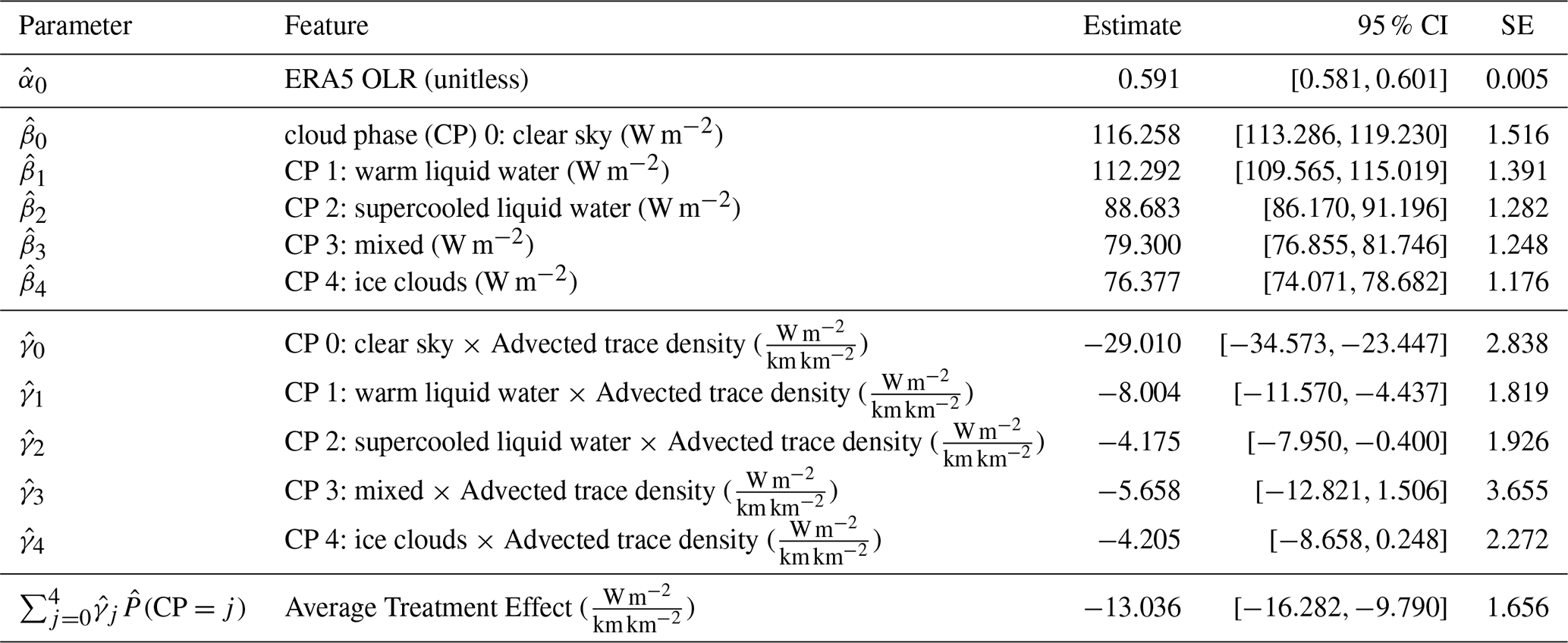
This sequence of unit conversion steps is therefore equivalent to multiplying by 3.6 to yield our central estimate:

$$\begin{array}{}\text{(5)}& \begin{array}{rl}& -\mathrm{13.036}{\displaystyle \frac{\mathrm{W}{\mathrm{m}}^{-\mathrm{2}}}{\mathrm{km}{\mathrm{km}}^{-\mathrm{2}}}}\cdot \mathrm{3.6}\\ & =-\mathrm{46.9}\mathrm{GJ}{\mathrm{km}}^{-\mathrm{1}}[-\mathrm{35.2},-\mathrm{58.6}].\end{array}\end{array}$$

Note that the sign being negative here is intentional: the regression slope being negative indicates heat is being trapped (i.e. when OLR is smaller, not as much thermal radiation is escaping into space). Elsewhere in this work we report our central estimate 46.9 GJ km⁻¹ consistent with the typical sign convention of earth system studies where positive numbers are warming.

Beyond the average treatment effect, one could hope to glean insights from the individual fitted coefficients of Table 1. The coefficient for the baseline ERA5 OLR (α₀ ≈ 0.59) shows an (expected) strong positive correlation with the COIN OLR. The fact that the estimate is substantially less than 1.0 indicates there remains a systematic scaling difference between the two OLR products even after the model accounts for the observed cloud states identified by GOES-16 L2 Cloud Phase product. The clear sky interaction with advected trace density is perhaps surprisingly the largest magnitude of the ${\widehat{\mathit{\gamma }}}_j$ coefficients; one might expect the ${\widehat{\mathit{\gamma }}}_{\mathrm{3}}$ mixed phase and ${\widehat{\mathit{\gamma }}}_{\mathrm{4}}$ ice clouds to be largest, if the underlying cloud phase data were accurately identifying the top phase as ice in the cloudy pixels that contain contrail forcing. However, Jiménez (2020) analyzed the GOES-16 Cloud Mask product accuracy compared to lidar ground truth measurements from CALIPSO and found that overall the clear sky detection accuracy was only 74.8 %. Figure 8 from Jiménez (2020) in particular shows that in the winter in some higher latitudes (where contrail formation rates are expected to be relatively high due to lower temperatures coinciding with large amounts of flight traffic in the northern half of the United States) the clear sky detection accuracy can be as low as 35 %, providing a plausible explanation for the large magnitude of ${\widehat{\mathit{\gamma }}}_{\mathrm{0}}$. To test this hypothesis, we performed a sensitivity analysis which shows a clear inverse relationship between the classification accuracy and estimation error (see Appendix C for full details). Considering the (possibly unexpected) nonzero values of ${\widehat{\mathit{\gamma }}}_{\mathrm{1}}$ and ${\widehat{\mathit{\gamma }}}_{\mathrm{2}}$ for water clouds, we note that again uncertainties in the Cloud Phase classification are a likely explanation: contrail cirrus optical depth only rarely exceeds 1.0 (Kärcher et al., 2009) and the validations performed by Pavolonis (2020) indicate the accuracy of “Optically Thin” or “Multilayered Ice” cloud classification is relatively poor, ranging from 39 %–58 %.

3.3 Estimation of contrail lifespan

We can utilize the advection age dimension of the advected trace density field to analyze how much longwave forcing is associated with each advection age. To do so we fit the 12 separate models from Eq. (3), each using as the treatment only the advected trace density which was younger than hour H (where $H\in \left\{\mathrm{0},\mathrm{\dots },\mathrm{11}\right\}$), estimating the longwave radiative forcing occurring as a result of air traffic less than H hours after aircraft passage. The violin plots generated in this manner are shown in Fig. 10. Notably, while Fig. 9 shows that the downward trend has mostly flattened by H ≥ 10 (correctly identifying that the synthetic groundtruth has little longwave forcing from contrails older than 9 h) in Fig. 10 we see that the violin plots continue downward until at least 12 h. This may indicate the observable average longwave forcing from contrails continues for more than 12 h after aircraft passage.

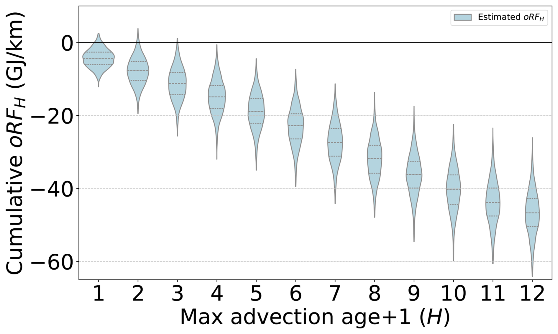
Figure 10 The estimated cumulative longwave forcing from contrails over the Americas as a function of cumulative advected trace density age (A_H). Each violin in the plot shows a distribution of the estimated forcing (oRF_H) from one of the twelve separate OLS fits, one for each cumulative age $H\in \left\{\mathrm{0},\mathrm{\dots },\mathrm{11}\right\}$. While we caution against interpreting the change between any pair of oRF_H=h and oRF${}_{H=h+\mathrm{1}}$ as being the marginal longwave forcing in contrails having that age, we note that the progression of violin plots shows a continued downward trend up to at least 12 h. The central estimate at 12 h is 46.9 GJ km⁻¹.

Note that due to correlations between A_H=h and $A_{H=h+\mathrm{1}}$, we caution against interpreting the change between any pair of oRF_H=h and oRF${}_{H=h+\mathrm{1}}$ as being the marginal longwave forcing in contrails having age H, and we are not performing multiple linear regression. Our analysis is similar to a sensitivity study or model comparison: we are visualizing how the cumulative effect estimate evolves as the time window for advection expands.

4 Discussion

4.1 Contextualizing the Forcing Estimate

We have provided here comparisons with CoCiP estimates of instantaneous radiative forcing (iRF), but the method we use here is not in fact estimating the exact same quantity. CoCiP estimates reported in this work (and in almost all of the literature to date) are executed in an “offline” mode, where the contrails modeled by CoCiP do not interact with the simulated atmosphere (as instantiated here in the ERA5 numeric weather data). Because of this, offline CoCiP estimates do not include feedback effects such as dehydration of the upper troposphere. These feedback effects have been noted to decrease the efficacy of contrail radiative forcing, and so climate simulations which take them into account have been reported as “Effective Radiative Forcing” (ERF) (Lee et al., 2021; Bickel et al., 2025) Because our method is driven by satellite observations of the real Earth's atmosphere, arguably it contains the first 12 h of such feedback effects, and so is not strictly an instantaneous radiative forcing. Considering one of the reported largest magnitude feedback effects (dehydration at flight levels, where decreased humidity – entrained into ice crystals of contrail cirrus and sedimented to lower altitudes – then decreases formation rates of natural cirrus), we do expect that some fraction of it is accounted for in the contrail forcing estimates reported in this work.

In Appendix E we further study the dependence of our observed warming on local hour, finding differences between the observational results and CoCiP simulations in Fig. E1b. It may be the case that such a flight-level dehydration effect is responsible for differences between the oRF_H=3 estimate and the “offline” CoCiP estimate seen in Fig. E1b. In support of that explanation, we note the diurnal timing is fairly consistent with the timing of the drop in linear contrail coverage sensitivity seen in Fig. 2 of Meijer et al. (2022). However, there are potentially multiple other artifactual (non-physical) explanations for the discrepancies between oRF estimates and CoCiP, detailed in Appendix E. Given that in the synthetic testbed shown in Fig. E1a the causal inference method is able to successfully recover the known synthetic ground truth diurnal curve, we conclude the explanation for the discrepancies in Fig. E1b is likely to lie in some remaining difference(s) between the synthetic testbed data and the data derived from real aircraft trajectories in the observed earth atmosphere. To distinguish which effects contribute to which degree, future work may need to explore even more realistic synthetic test data, that is specifically designed to include more realistic correlations of aircraft trajectories with respect to natural clouds and/or generating more realistic distributions of environmental confounder variables than are available by a simple latitude flipping of flight paths.

While 12 h estimates we provide here are unlikely to account for any Nitrous Oxide (NO_x) driven feedback effects, since they are expected to require multiple days of atmospheric chemistry reactions to become evident (Brasseur et al., 2016), it has not currently been reported what fraction of the full dehydration feedback effect is captured by oRF_H=12 estimates. The closest source from which to currently speculate may be CO₂ climate modeling studies, for example Dong et al. (2009) reports in some study variants that cloud rapid adjustment response was “statistically consistent with the equilibrium value” by day 5 after the perturbation. Considering that our reported forcing is not quite iRF and not quite ERF, we propose for clarity of comparisons between contrail forcing estimate types that observation-driven analysis of contrail forcing can adopt the term “Observational Radiative Forcing” with a subscript of the number of hours traced in the observations, e.g. this work reports oRF_H=12.

There has been one report in the literature of CoCiP estimates being executed in an “online” mode, where it is coupled with the simulated atmosphere: Schumann et al. (2015) reports a 15 % reduction in efficacy of contrail radiative forcing due to the dehydration effect. Taking this effect into account and applying a 15 % reduction to CoCiP's offline estimate of 60.7 GJ km⁻¹ on the analysis region from this work puts the CoCiP estimate within our observation-based estimate's confidence interval (35.2 to 58.6 GJ km⁻¹).

The average lifespan we estimate of 12 or longer hours is a somewhat longer average lifespan than expected based on the CoCiP simulations of these same flights. It is possible this is due to CoCiP only modeling the fall streak portion of the contrail and not the smaller ice crystals of the contrail which sediment more slowly or not at all, as hypothesized recently by Akhtar Martínez et al. (2025). It may also in part be an artifact of our analysis: as seen in Fig. 9a, b and c the blue “Estimated oRF_H” curves do not align perfectly with their respective orange synthetic “Ground truth” curves. We suspect the misalignment is due to correlations across adjacent hours H of the advected trace density, where the contrail forcing from any given hour H is also strongly correlated with adjacent hours and the causal model has no available counterfactual data to discriminate which hour it should be attributed to. It is possible that a causal model which explicitly tracks temporal state changes such as was used in Fons et al. (2023) may yield an improved lifespan estimate.

4.2 Limitations and Future Work

A notable limitation of this approach is that it relies on aggregations of large numbers of flights and independent background weather systems to estimate an average treatment effect. In future work it may be able to estimate average effects of coarse subgroups such as airline, region, or engine types, but we do not expect the approach as currently devised to be able to observationally discern the radiative forcing of one individual contrail, nor to be able to separate pixels observed in satellites into categories of “contains contrail cirrus” versus those that instead “contain natural cirrus”.

We generally expect Ordinary Least Squares estimates to be robust in the presence of independent measurement bias (Wooldridge, 2016): in this case, bias in COIN OLR. This is confirmed here to some degree with the “Measurement bias” variation of the synthetic tests described in Sect. 2.5. However, OLS may not be robust to biases in confounder control variables (Wooldridge, 2016); here, these are the ERA5 OLR and GOES-16 Cloud Top Phase product, so in the future it would be ideal to control with observational data that accounts for multiple cloud layers such as the GOES-R Cloud Cover Layer product (GOES-R Algorithm Working Group and GOES-R Series Program, 2023). Unfortunately that product is only available starting in May 2023 and does not coincide with the timespans when we have purchased satellite ADS-B data that is crucial for generating accurate advected trace density over ocean regions. Additionally it would be ideal to also include observational data with improved accuracy for optically thin ice clouds; machine-learning approaches such as Kox et al. (2014) that are specifically developed for ice clouds hold the most promise in our view.

Additionally there is a potential source of unmeasured confounding that remains, in the non-random nature of flight routing. Aircraft systematically avoid turbulent regions for safety, and the atmospheric dynamics that generate this turbulence might have an association with natural cirrus clouds. Although including the GOES-16 Cloud Top Phase product in Eq. (1) partially accounts for this, the relationship between turbulence and observed cloud cover is not perfectly deterministic. Therefore, a subtle bias may be introduced, as the model might incorrectly attribute the radiative effects of these systematically avoided cloudy regions to the absence of air traffic. Future work could aim to address this more explicitly by incorporating turbulence forecast data as an additional predictor.

We also anticipate future refinements in advected trace density: while our current model assumes a linear growth in wind error uncertainty, a more sophisticated state-dependent error model could be developed where the error varies with geographic location, altitude, and local meteorological conditions like wind shear. Another advancement of wind uncertainty might be to calculate per-waypoint uncertainty based on performing advections in multiple weather ensemble members as done by Meijer (2024). Such improvements could reduce the spatial uncertainty of aged contrails and could sharpen the resulting forcing estimates, particularly for contrails with longer lifetimes.

Our introduction of oRF_H=12 motivates targeted climate model experiments to better connect observational results with long-term climate impacts. By running climate simulations for 12 h, one could quantify the forcing after only rapid atmospheric adjustments from this time interval have occurred. This may allow computing the ratio between iRF and oRF_H=12, which could then be compared to reported iRF $/$ ERF ratios. This could illustrate how much of the total adjustment from iRF to ERF occurs within the first 12 h and the degree to which short-term observational metrics like oRF_H=12 can constrain the full climate response.

A crucial future extension of this methodology is to analyze the shortwave radiative effects of contrails to determine their net radiative impact. This requires quantifying the cooling effect from reflected solar radiation (RSR), which presents a more difficult challenge than the longwave analysis in this study: CoCiP and climate model estimates suggest contrail RSR signal will be smaller in magnitude than the longwave forcing (for example in our study domain CoCiP estimated 60.7 GJ km⁻¹ for longwave forcing and −32.1 GJ km⁻¹ for shortwave forcing). At the same time it is embedded within a much larger background variance: see Fig. 3 in McCloskey et al. (2023b) for typical ranges of OLR and RSR. Additionally, RSR has a few more potential confounders than OLR: diurnal and annual cycles of solar illumination, stronger dependence on viewing angle including sunglint from water surfaces, and stronger dependence on surface type and potentially on cloud aerosol interactions. Therefore it may be required to reduce wind uncertainty to strengthen the correlations of the treatment (advected trace density) with the outcome (change in RSR), and thorough feature engineering of confounder inputs in regression models is likely needed.

In the meantime, it may be tempting to consider the estimated 46.9 GJ km⁻¹ longwave component of the forcing to be an upper bound magnitude of the average net forcing per flight kilometer, but some cautions are advised. For example, it is possible (based on Fig. D1) that our estimate is an under-estimate of the magnitude of the longwave forcing, and further investigation may develop methodology with an improved calibration that revises the estimated forcing to be a larger magnitude. It is also possible that in future applications of this technique with improved confounder controls (for example more accurate cloud satellite data products) the longwave forcing estimate may change (see Appendix C for sensitivity study). And finally, future work quantifying the impact of the uncontrolled confounding of aircraft trajectories preferring clear skies may also result in revising the estimated longwave forcing to be a larger magnitude.

Another important extension of this work is to apply this analysis to global satellite observations; the current study is limited to the Americas, and its air traffic patterns and meteorological conditions may not be representative of global aviation. Similarly, given the high inter-annual variation reported for contrails, analyzing data from more years will be valuable. Additionally this framework can be extended to perform detailed subgroup analyses beyond the fleet-wide average: by partitioning the dataset by engine type, local time of day, geographic region, or specific synoptic weather patterns, we could identify which flight and weather categories contribute disproportionately to contrail warming.

5 Conclusions

In this work, we provided a large-scale, observation-driven estimate of long-lived contrail radiative forcing. Our approach, grounded in a causal inference framework, successfully isolates the average contrail longwave radiative forcing signal from confounding weather effects by combining high-resolution satellite observations with flight data, thereby avoiding the limitations of traditional linear contrail masks. Our analysis quantifies the longwave 12 h observational radiative forcing (oRF_H=12) to be 46.9 GJ km⁻¹ and suggests that average contrail longwave radiative impact may exceed 12 h. This work provides a new way for observationally estimating an important component of aviation's non-CO₂ impact and demonstrates an approach that could be used to validate atmospheric models and potentially evaluate future mitigation strategies.

Appendix A: Sublinear overlap formula

We generate a variation of a synthetic validation test to investigate whether estimations using a linear function introduces estimation error when the effect on OLR with overlapping contrails is likely to be somewhat sublinear in reality. To do this we generate synthetic data using a sublinear overlap function in pixels where multiple contrails from distinct aircraft are estimated by CoCiP. In typical CoCiP estimations of contrail forcing, the RF from these separate contrails would be linearly summed. Here instead we approximate the contrail RF effect via the sum of the optical depths.

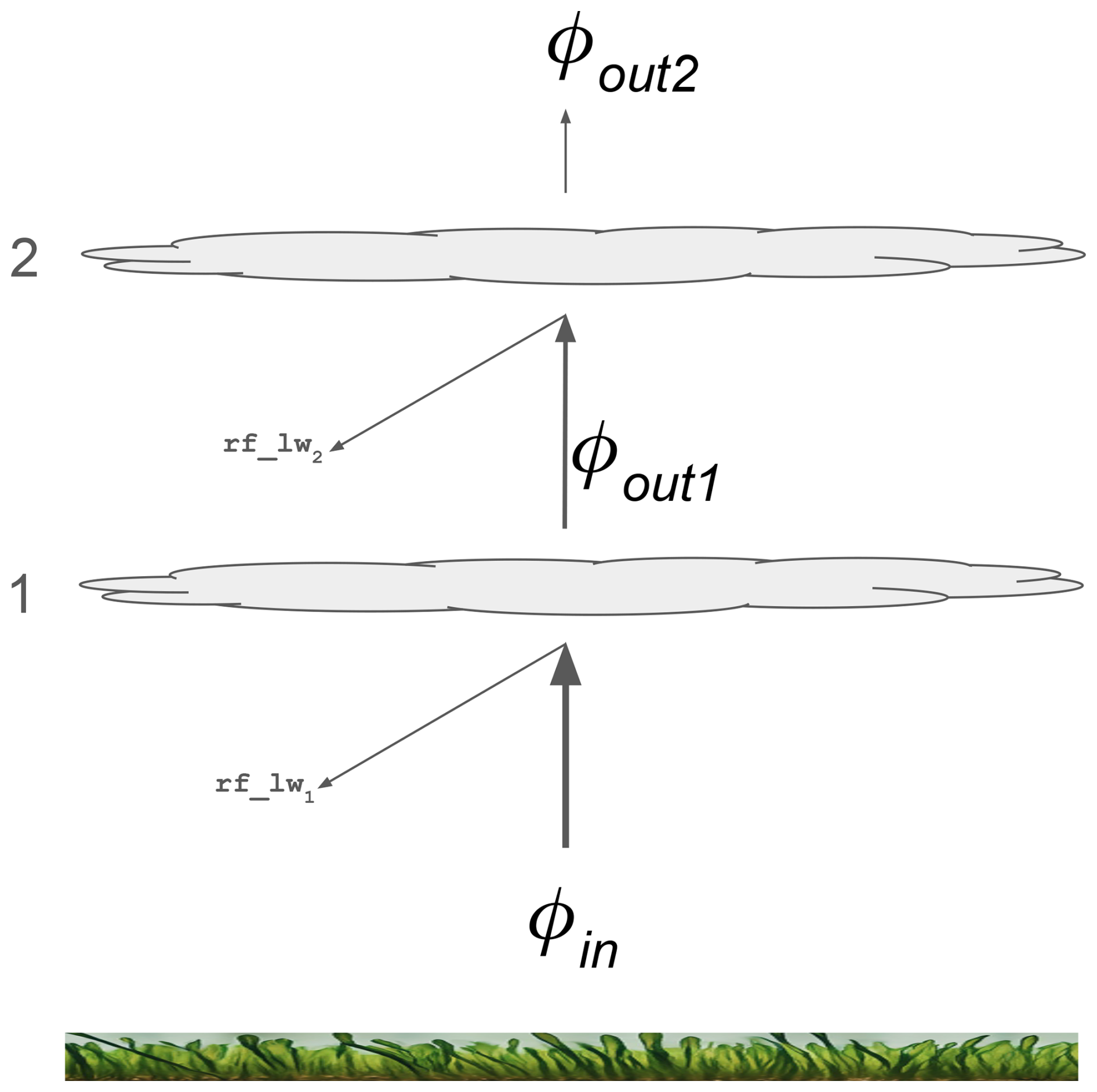
Figure A1 Sublinear overlap of contrail radiative forcing used in one synthetic validation test. ϕ_in is the initial upwelling irradiance, here estimated by COIN in W m⁻². After contrail 1 has attenuated the flux it becomes ${\mathit{\varphi }}_{{\mathrm{out}}_{\mathrm{1}}}$ and after attenuation from contrail 2 it becomes ${\mathit{\varphi }}_{{\mathrm{out}}_{\mathrm{2}}}$, which in the case shown would be the “satellite-observed” synthetic OLR since contrail 2 is the highest cloud.

The diagram Fig. A1 shows two distinct contrail layers, having optical depth τ₁ and τ₂ respectively. Given that optical depth is defined as:

$$\mathit{\tau }=\ln \left({\displaystyle \frac{{\mathit{\varphi }}_{\mathrm{in}}}{{\mathit{\varphi }}_{\mathrm{out}}}}\right).$$

To calculate the top level OLR (${\mathit{\varphi }}_{{\mathrm{out}}_{\mathrm{2}}}$) we can see:

$${\mathit{\varphi }}_{{\mathrm{out}}_{\mathrm{2}}}={\displaystyle \frac{{\mathit{\varphi }}_{{\mathrm{out}}_{\mathrm{1}}}}{e^{{\mathit{\tau }}_{\mathrm{2}}}}}={\displaystyle \frac{\frac{{\mathit{\varphi }}_{\mathrm{in}}}{e^{{\mathit{\tau }}_{\mathrm{1}}}}}{e^{{\mathit{\tau }}_{\mathrm{2}}}}}={\displaystyle \frac{{\mathit{\varphi }}_{\mathrm{in}}}{e^{{\mathit{\tau }}_{\mathrm{1}}}{e}^{{\mathit{\tau }}_{\mathrm{2}}}}}={\displaystyle \frac{{\mathit{\varphi }}_{\mathrm{in}}}{e^{\left({\mathit{\tau }}_{\mathrm{1}}+{\mathit{\tau }}_{\mathrm{2}}\right)}}},$$

which in the general case of n distinct contrails in the same pixel results in the formula we use to generate the “Sublinear overlap” variant of the synthetic test data:

$$\begin{array}{}\text{(A1)}& {\mathit{\varphi }}_{{\mathrm{out}}_n}={\displaystyle \frac{{\mathit{\varphi }}_{\mathrm{in}}}{e^{\left({\sum }_{i=\mathrm{1}}^n{\mathit{\tau }}_i\right)}}}.\end{array}$$

Appendix B: Pixel area calculation

GOES-16 ABI longwave pixels have a nominal (nadir) size of 2 km per side but are larger than that at longer viewing angles. In this work we estimate the contrail longwave forcing in units of GJ km⁻¹ (gigajoules per flight km) based on input quantities that are initially normalized by area (e.g. W m⁻²) and so (both in synthetic validation tests to calculate ground truth and in the forcing estimates themselves) it is necessary to weight by pixel area. GOES-16 data are not provided with pixel area, but we utilize the latitude and longitude of pixel centers provided in the GOES-16 ABI L1b radiances data product to make a close approximation of the pixel area for each pixel in the ABI pixel grid. Using the notation from Fig. B1, we calculate the area of the pixel centered on C based on the pixel centers A, B, C making a triangle (ABC). The triangle side lengths a, b are calculated using great circle distance along the surface of the earth as approximated by a sphere with radius = 6371 km. The interior angle γ can then be found using the Law of Cosines (i.e., γ = ${\cos }^{-\mathrm{1}}\left(\frac{a^{\mathrm{2}}+b^{\mathrm{2}}-c^{\mathrm{2}}}{\mathrm{2}ab}\right)$) and finally the pixel area as a function of a, b, γ comes from the formula for area of the parallelogram ADBC = $a\cdot b\cdot \sin \left(\mathit{\gamma }\right)$.

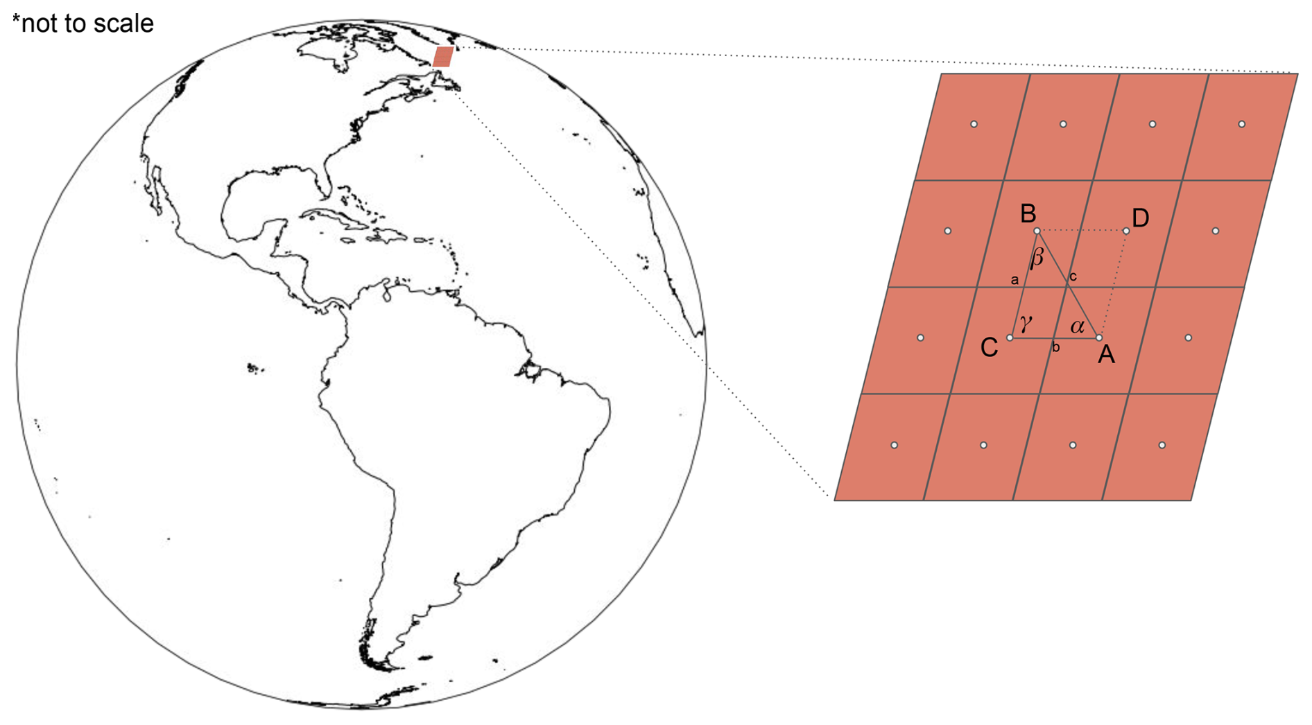
Figure B1 Notation used in formula for calculating GOES-16 ABI pixel area. The brown enlarged inset represents a portion of the ABI pixel grid with white dots on pixel centers.

Appendix C: Sensitivity of oRF_H=12 to Ice Cloud Phase Misclassification

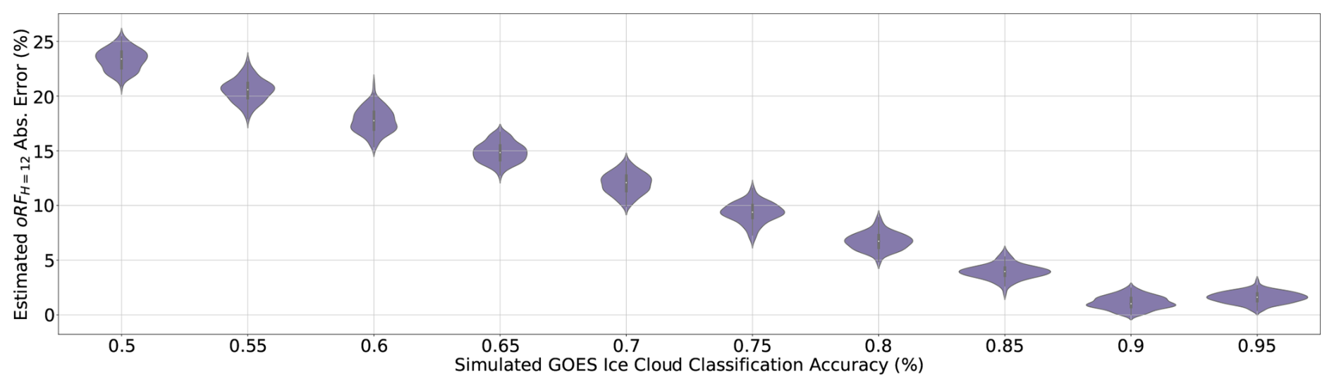
Figure C1 Distribution of the absolute percentage error in the estimated longwave oRF_H=12 as a function of the simulated accuracy of the GOES ice cloud classification. The analysis was performed on the synthetic dataset where the true radiative forcing is known. The results demonstrate that as the accuracy of the cloud phase input improves, the error in the final longwave forcing estimate systematically decreases.

To address the potential impact of known inaccuracies in the satellite-derived ice cloud phase product on our final estimate, we performed a sensitivity analysis using our linear overlap synthetic dataset. As noted in the main text, satellite algorithms can misclassify optically thin ice clouds (such as contrails) as clear sky, which could influence the partitioning of the contrail effect across the model's coefficients. This analysis quantifies the sensitivity of our estimated oRF_H=12 to the misclassification rate. To do this we use the synthetic dataset where the ground truth radiative forcing is known for every pixel containing a synthetic contrail. We then systematically vary a “Simulated GOES Ice Cloud Classification Accuracy” parameter from 50 % to 95 %. This parameter represents the probability that a pixel containing a synthetic contrail is correctly labeled as an “ice cloud” (Cloud Phase 4) before being passed into our OLS regression model. If not labeled as an ice cloud, the pixel retains its original classification. To assess the uncertainty for each accuracy level, we generated a distribution of oRF_H=12 estimates. This was achieved by running our causal inference regression (Eq. 1) 100 times, with each run performed on a new random sample of 100 000 pixels drawn with replacement from the dataset. Finally, we calculate the absolute percentage error between our model's estimates and the known synthetic ground truth (both in GJ km⁻¹ units). Figure C1 shows the results of this analysis. The violin plots illustrate the distribution of estimation errors for each simulated accuracy level.

The results demonstrate an inverse relationship between the accuracy of the ice cloud phase classification and the error in our final forcing estimate. As the simulated accuracy improves from 50 % to 90 %, the median absolute error decreases from approximately 24 % to less than 2 %. This analysis provides quantitative support for the hypothesis that the large coefficient observed in the clear-sky category (${\widehat{\mathit{\gamma }}}_{\mathrm{0}}$ in Table 1) is substantially influenced by cloud phase misclassification. Furthermore, it demonstrates the robustness of the method: even at realistic accuracy levels reported in the literature (e.g., 75 %), the estimation error remains reasonably constrained.

Appendix D: Poor signal:noise ratio can cause attenuation

We take advantage of the synthetic testbed described in Sect. 2.5 to arbitrarily scale the magnitude of the CoCiP longwave forcing which is rasterized on top of COIN OLR and used as groundtruth in these synthetic validations. Figure D1 shows an attenuation effect, where smaller magnitudes of groundtruth longwave forcing such as 10 or 20 GJ km⁻¹ have their magnitudes under-estimated by about 10 GJ km⁻¹.

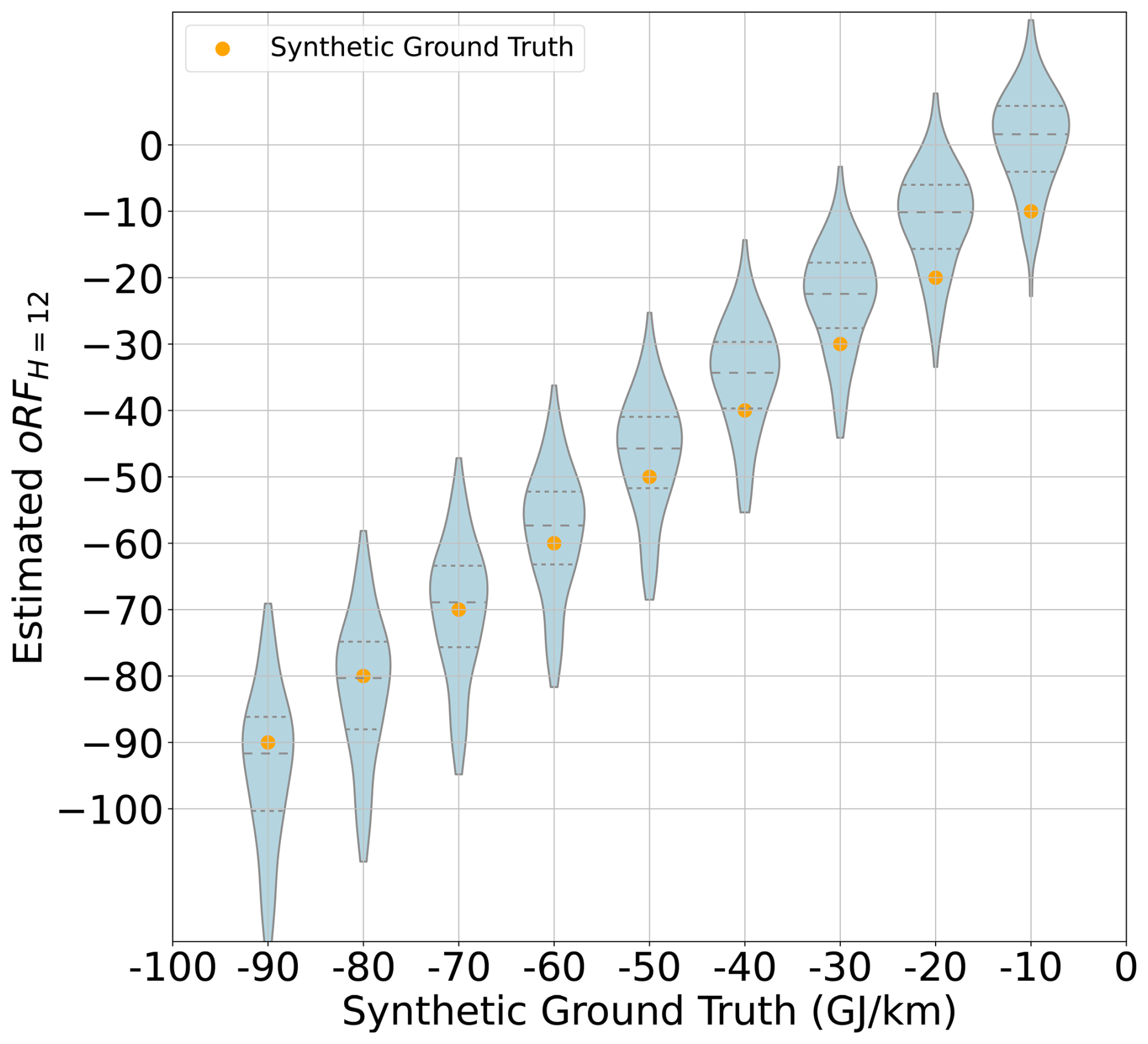
Figure D1 The result of systematically varying the synthetic groundtruth magnitude of longwave forcing in the “Linear overlap” synthetic dataset. Each violin represents 100 bootstrap estimates of oRF_H=12 for the given x-axis value of longwave forcing. While the inter-quartile range of the oRF_H=12 estimates contain the synthetic ground truth value when the synthetic groundtruth magnitude is at least ≈ 40 GJ km⁻¹, the trend of central estimate oRF shows a clear attenuation, under-estimating the magnitude of the longwave forcing on smaller values.

This highlights the value of using synthetic validations in causal modeling efforts. For example, future analysis on subgroups of flights may have individual subgroups that have low-magnitude forcing; or in estimations of shortwave forcing from contrails which models have indicated are of smaller magnitude on average than the longwave forcings. Validating that regression estimates are well calibrated in the relevant effect size ranges would give confidence in the correctness of the results.

Appendix E: Conditional Average Treatment Effect and the Diurnal Cycle

The causal inference methodology can be further explored to do a more fine-grained analysis where instead of estimating an overall effect of contrails on OLR (the ATE), this effect can be disaggregated by different subgroups of interest. In the causal inference literature this is referred to as Conditional Average Treatment Effect (CATE) as it estimates the effect conditioned on a subgroup of the data (Abrevaya et al., 2015). Depending on the chosen subgroups, the CATE can illustrate how impact differs over land versus water, by geographical regions, by time of day, and – signal-to-noise ratio permitting – by airline or aircraft engine type. However, achieving a robust causal estimate for each subgroup requires careful model building and ideally specialized synthetic tests to validate it. We use a diurnal cycle case study to exemplify both the potential of the method and the complexity of the causal interactions that one must consider when performing fine-grained analysis.

E1 Diurnal Cycle CATE

By performing regressions on pixels that are limited to a particular local hour of the day, we can showcase how to come up with a CATE of the diurnal cycle of contrail forcing. The local hour timezone offset from the UTC time of the observation of the pixel is approximated as a function of the pixel's longitude (each 15° of longitude are grouped as a 1 h timezone). We performed 24 separate regressions, each fitting Eq. (1), and compared the resulting GJ km⁻¹ h⁻¹ values to the offline CoCiP estimated forcing rasterized in those same pixels (Fig. E1). Note the x axis is 48 h long because the same 24 results have been concatenated back-to-back to give a more intuitive visualization of the trend lines.

At a first glance of Fig. E1a, the causal model successfully captures the synthetic ground truth of the diurnal effect stratified by local hour of day. However, when we apply this technique to the real dataset (Fig. E1b), some potentially non-physical artifacts become apparent. For example, the estimated impact at local noon closer to 0 GJ km⁻¹ h⁻¹ than what is estimated by the offline CoCiP model. Additionally, at local midnight and after, the effect is occasionally larger in magnitude (more longwave forcing) than what is estimated by the offline CoCiP model.

As discussed in Sect. 4.1, oRF might be smaller in magnitude than the offline CoCiP iRF because our observational method captures negative atmospheric feedback effects, such as dehydration of the upper troposphere, which decreases the efficacy of contrail radiative forcing. This could contribute to explaining the parts of the diurnal trend where the oRF curve is closer to zero (less longwave forcing) than the CoCiP curve in Fig. E1b. We believe it is likely to also be affected by attenuation artifact described in Appendix D and the effect of varying data quality and confounding as a function of the local hour strata.

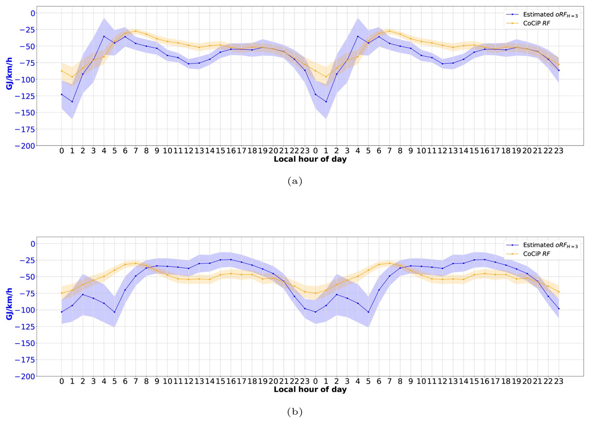
Figure E1 The diurnal cycle of contrail longwave forcing. The plot shows the estimated forcing (GJ km⁻¹) by CoCiP and causal inference regression (oRF_H=3) for each approximate local hour of the day, for (a) the “Linear Overlap” synthetic test and for (b) real contrail forcing estimated over the Americas. The approximate local hour of the day is determined by treating each 15 ° of longitude as grouped into a 1 h “timezone”). The x axes include 48 ticks because the same 24 h of data are repeated in order to better visualize the diurnal trend. Note the flight km used to normalize all estimates is from advected trace density up to at most 3 h old, to allow a temporally localized comparison. This illustrates how the longwave forcing of contrails varies between day and night. We note that in panel (b) the oRF_H=3 estimate differs from CoCiP's estimate primarily in the local mid-day and afternoon; this is likely due to one or more differences between the synthetic testbed and the real data over the Americas. For example, it may be due to uncontrolled confounding, or an atmospheric dehydration effect that is not modeled by CoCiP. Mid-day differences between CoCiP and oRF_H=3 are also likely impacted to some degree by the attenuation effect described in Appendix D.

E2 Complexity and Potential Bias Introduced by Subgroup Analysis

There are a few ways in which stratifying the analysis by local hour might introduce non-physical artifacts and biases that are diluted or absent in the marginal (aggregate) analysis (Wooldridge, 2016).

Stratifying the observations by time of day might introduce uncontrolled confounding caused by non-random routing of flight traffic. The most notable risk in our opinion is a concentration of unmeasured confounding within a few hourly bins. Aircraft systematically avoid dynamic and turbulent regions, notably mid-day convective clouds. This introduces a difference (a “selection effect”) between areas with air traffic and similar areas without it. When performing the regression specifically at and around local hour 13:00, the analysis is restricted to a sample where aircraft tend to selectively fly over clearer skies more often (Honomichl et al., 2013; Guan et al., 2001). The model may incorrectly attribute the lower OLR (higher longwave forcing) of these avoided cloudy regions to the absence of air traffic – and conversely also incorrectly attribute the higher OLR (lower longwave forcing) of the clear-sky areas to increased presence of air traffic – which would have the effect of pulling the hourly forcing estimate toward zero. In the aggregate ATE calculation, this bias is dampened by being averaged with the rest of the hours where convective avoidance is less frequent. The main ATE result (46.9 GJ km⁻¹) integrates over the distribution of these “flight traffic : cloud” interactions which mitigates the risk of biased estimates.

Measurement error in covariates as a function of time of day can also introduce non physical artifacts. The accuracy of key satellite inputs – the confounder controls – can vary with the solar cycle (local hour/Solar Zenith Angle). For example the GOES-16 Cloud Phase data product relies on different spectral channels and algorithms for pixels in daylight (visible/NIR) versus night (infrared) (Li et al., 2023; Pavolonis, 2020; Jiménez, 2020). Optically thin ice clouds, such as contrails, have been noted as difficult to classify, and this difficulty increases when retrieval angles are complex or when the algorithm switches modes (e.g., twilight) Kärcher et al. (2009). The resulting time-dependent misclassification rate directly impacts the ${\widehat{\mathit{\gamma }}}_j$ coefficients when estimating local-hour CATE. If for example the cloud phase accuracy dropped at night, the contrail forcing could mistakenly be assigned to incorrect ${\widehat{\mathit{\gamma }}}_j$ coefficients, which can become volatile and potentially physically implausible.

To help quantify the effects of some of these issues, we apply here the hat-value diagnostic described by Moodie and Schulz (2025). The “positivity assumption” being assessed by the diagnostic dictates that subgroups in a trial/study need to have both a meaningfully positive probability of being exposed to the treatment and not exposed to treatment. That is in this case, subgroups having advected trace density (A_H > 0) or not (A_H = 0). A “positivity violation” is then referring to a subgroup that has such a low/high probability of being exposed to treatment that no data exists in the dataset to allow inference of what would have happened in the counterfactual case. When applying the hat-value diagnostic to the aggregated oRF_H=12 estimate dataset, no violations are detected. However, applying the hat-value diagnostic to each of the 24 local hour subgroups shown in Fig. E1b over the Americas, the local hours 5, 6, and 7 are reported as having positivity violations. This strongly implies further improvements are needed to be able to report low-bias estimates of longwave forcing scoped to those local hours.

The diurnal cycle analysis serves as a powerful illustration of the challenges of implementing a robust causal model in a space with varying levels of data quality and noise such as the atmospheric physics space. While the marginal ATE is resilient to these localized errors via aggregation (Wooldridge, 2016), further subgroup analysis conditioned on local hour would benefit from more advanced controlling of time-dependent confounding and subgroup-dependent measurement error, possibly by including turbulence forecasts/reanalysis as confounder controls and using cloud products with improved accuracy.