Long-term cloud characterization at the AGORA ACTRIS-CCRES station using a novel classification algorithm

The Western Mediterranean is a climatic hotspot with strong variability in cloud processes. However, Cloudnet sites there are scarce compared to northern Europe. This study presents for the first time a five-year cloud statistical analysis at the AGORA ACTRIS-CCRES station in Granada (Spain), using 94 GHz Doppler radar, microwave radiometer, and ceilometer data. Analyses focus on single-layer clouds and their interannual variability in macrophysical and microphysical properties. A new cluster-based algorithm (CBA) is introduced for cloud classification, reducing spurious correlations found in earlier methods. The CBA shows single-layer cloud minima in summer, with annual occurrences of 5.0 % for ice, 3.6 % for precipitating ice, 3.4 % for mixed-phase, 3.2 % for precipitating mixed-phase, and 1.4 % (1.2 %) for liquid (precipitating liquid) clouds. Liquid clouds are observed at 1–2 km, thin (∼ 200–300 m), with a droplet radius of 5 µm and liquid water paths of 12 g m⁻². Mixed-phase clouds occur at 5–6 km, nearly 1 km thicker, with larger droplets (10.8 µm) and ice water paths of 3.5 g m⁻². Ice clouds dominate at 7–8 km, the thickest type, with higher ice water paths (8.5 g m⁻²) but smaller particles (∼ 39 µm) than mixed-phase (∼ 45 µm). Across all phases, precipitating clouds have lower bases, greater thickness, and higher water content and particle sizes than non-precipitating clouds. These results provide benchmark data for satellite and model evaluation. The algorithm can be applied to other Cloudnet sites, supporting consistent European cloud statistics.

1 Introduction

Clouds play a vital role in regulating Earth's radiative budget. They interact with solar and thermal radiation, affecting the energy balance and, consequently, the surface temperature (Twomey, 1977). The hydrometeor phase, shape and concentration affect the interaction with solar and thermal radiation (Yoshida and Asano, 2005), posing a significant challenge to estimate their radiative effect as suggested by Dong et al. (2017) and Li et al. (2022). Additionally, the high spatial and temporal variability of clouds increases the difficulty of its study. Thus, clouds are still in the spotlight of the atmospheric science community (Forster et al., 2023). Additionally, they are part of the hydrological cycle, transporting moisture to various regions (Pruppacher and Jaenicke, 1995; Chagnon et al., 2004; Brueck et al., 2015). The transport and its inhibition can cause heavy rainfalls and the reduction of cloud fraction, respectively (Liu et al., 2018; Bishop et al., 2019; Nygård et al., 2019; Zhao and Zhou, 2021). These phenomenons are directly associated with floods and drought, which are intensifying in the Mediterranean Region (Rios-Entenza et al., 2014; Hoerling et al., 2012).

Passive satellite remote-sensing techniques have been used to explore cloud cover, providing a global picture of cloud properties. However, they present low temporal resolution and information on low level clouds is affected by large uncertainties (Kachar et al., 2015; Wieland et al., 2019). Moreover, satellite active methods such as those using Doppler radars remain challenging (Griesche et al., 2024), and require careful cal/val procedures (Protat et al., 2006, 2010). Thus, ground-based observations are necessary for improving the accuracy of cloud properties. Particularly, the Cloud Doppler Radar (CDR) can perform measurements of clouds with high-temporal and vertical resolution. It can provide information on cloud dynamics as well as the size, shape, phase and orientation of its hydrometeors (Li et al., 2021; Lamer et al., 2014; Griesche et al., 2019; Myagkov et al., 2016).

Several studies have been performed using CDR data in Europe, such as Li et al. (2021), Kalesse-Los et al. (2022) and Vogl et al. (2024), where spectral signal were analyzed in order to assess cloud droplets properties. The studies by Kneifel et al. (2022), Nomokonova et al. (2019), Bühl et al. (2016) and Achtert et al. (2020) performed statistical analysis of cloud properties using post-processed cloud remote sensing data provided by ACTRIS Cloudnet (ACTRIS: Aerosols, Clouds, and Trace gases Research InfraStructure), a European network dedicated to cloud remote sensing (Illingworth et al., 2007). These studies use the Cloudnet classification products to determine cloud phase with a profile-based algorithm (PBA) that classifies individual profiles. For example, Nomokonova et al. (2019) applied the PBA to characterize single-layer clouds at the Ny-Ålesund station; Kneifel et al. (2022) investigated ice cloud variability in the German Alps; and Pîrloagă et al. (2022) examined seasonal cloud variability in Bucharest using the PBA approach. Bühl et al. (2016) also used the PBA but extended it to selected intervals with more than 15 min with the same cloud profile. However, all these studies are based on measurements acquired in Northern Europe.

To address the gap of studies in South of Europe, the AGORA (Andalusian Global ObseRvatory of the Atmosphere) has been operating a 94 GHz CDR since 2018, providing long-term measurements of cloud properties on the Mediterranean basin, which is a key region for climate variability. AGORA is one of the southernmost ACTRIS-CCRES station, with database available in ACTRIS Cloudnet. Notably, it stands as the only cloud remote sensing database available in the Iberian Peninsula, making it an invaluable resource for regional climate studies. The study presented here aims to perform a statistical analysis on single layer clouds for more than half a decade of observations at the AGORA station, taking advantage of the available Cloudnet database. Statistical analyses of cloud macrophysics (e.g., cloud thickness, base and top height) and microphysics (e.g., liquid/ice water content and liquid/ice effective radius) are performed for different cloud types. To perform this classification, a novel algorithm based on the use of clusters is presented here. The cluster-based algorithm (CBA) also relies on the Cloudnet classification product and classifies types of clouds according to the percentage of hydrometeor phase within each cluster (e.g. ice, liquid or mixed-phase clouds), considering the composition of the entire volume occupied by the cloud. Roschke et al. (2024) used a cluster approach similar to ours, but with a different classification scheme, separating clusters into warm and cold clouds for the Barbados site.

The experimental site, datasets, instruments and products are described in Sect. 2. The proposed new approach on cloud classification algorithm and the cloud assessment are presented in Sect. 3. Section 4 reports monthly statistics of cloud occurrence, seasonal statistics of cloud base, top, and thickness. In addition, this section discusses the liquid and ice microphysical properties variability for different clouds. Finally, Sect. 5 summarizes the main findings and discusses their importance to improve further cloud statistics analysis.

2 Experimental site and database

AGORA (Global Atmospheric Observatory of Andalusia, at 37.16° N, 3.61° W, 680 m a.s.l.) is located in the South of the Iberian Peninsula being one the most meridional ACTRIS-CCRES station. This station is part of Cloudnet since 2018 and was integrated into ACTRIS-CCRES in 2023 as an ACTRIS national facility. The region experiences a continental climate with Mediterranean influence, having colder months in winter and spring, and warmer months in summer and fall. According to Bedoya-Velásquez et al. (2019), temperature below 5 km above ground level (a.g.l.) ranges between 10–20 °C during winter, and 20–40 °C during summer. On the other hand, the relative humidity ranges between 60 %–75 % in winter, and 40 %–50 % in summer (Navas-Guzmán et al., 2014). The region is also affected by North African, Atlantic and Mediterranean air masses, with sporadic events from the Mediterranean and continental Europe (Pérez-Ramírez et al., 2016). This, plus the influence by the Azores high, ultimately determine the meteorological conditions in the station.

2.1 Instrumentation

The AGORA observatory operates multiple instruments (Abril-Gago et al., 2023; Ortiz-Amezcua et al., 2022) in the framework of ACTRIS-CCRES, being their main characteristics summarized in Table 1. This includes operational frequencies or wavelengths, type of measurements, products, measurement ranges, data collection intervals, and references for more details. A brief description is provided below.

The dual polarimetric RPG-FMCW 94 GHz CDR named NEPHELE, measures the Doppler Velocity Spectrum (DVS) of hydrometeors for horizontal and vertical linear polarizations at 94 GHz. The instrument is used to compute the reflectivity (Z), mean Doppler velocity (ν_D), and spectral width (S_ω) of these particles. NEPHELE also derives the linear depolarization ratio (LDR), enabling the detection of the melting layer, aerosols, and insects as described by Hogan and O'Connor (2006). In addition, the radar has a passive channel for deriving an estimate the liquid water path (LWP). Its principal characteristics are the frequency-modulated continuous wave (FMCW) signal, which allows different range and time configurations (see Table 1). More details can be found in Küchler et al. (2017).

The RPG-HATPRO G2 (Humidity and Temperature PROfiler) microwave radiometer (MWR) is a passive remote sensing instrument that measures the brightness temperature (T_B) in the 22–31.4 and 51–58 GHz ranges. The first range covers the water-vapor absorption band and a window channel near 31.4 GHz, which is sensitive to liquid water. The second range covers the oxygen absorption band. LWP (see Table 1) is mainly retrieved from the 31.4 window and the water-vapor channels. The radiometric accuracy is 0.3–0.4 K, and integration time of 1 s. More details can be found in Navas-Guzmán et al. (2014) and Rose et al. (2005).

The CHM15k Nimbus ceilometer is an active remote sensor that utilizes a vertically pointed Nd:YAG pulsed laser to measure backscattered photons by aerosols and cloud droplets. The instrument is used to retrieve the attenuated backscattering coefficient (β_att) of aerosols and small cloud droplets. It operates at repetition frequency intervals of 5–7 kHz, where each pulse is emitted at 1064 nm with 8.4 µJ of energy. The temporal and vertical resolutions are 15 s and 15 m, respectively, and the full overlap is reached roughly at 1500 m a.g.l. (Heese et al., 2010). More details can be found in Cazorla et al. (2017).

Küchler et al. (2017)Navas-Guzmán et al. (2014)Cazorla et al. (2017)

Table 1 Instrument specifications and data products of the AGORA ACTRIS-CCRES station.

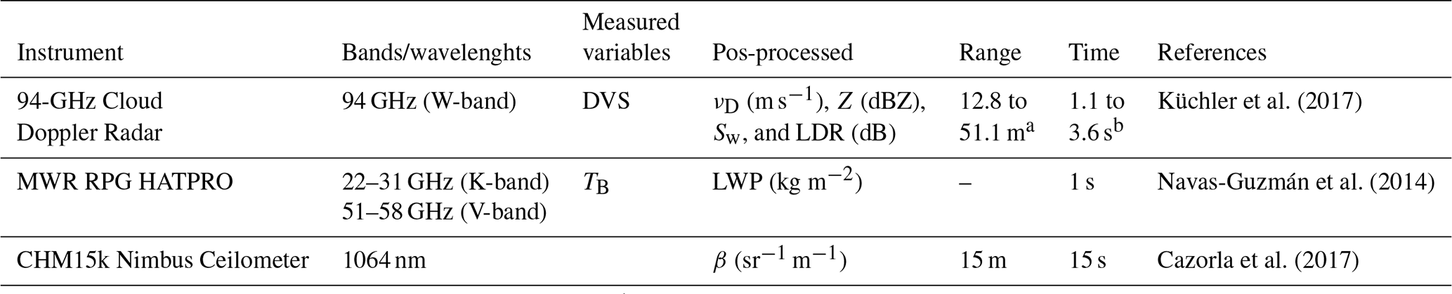
^a This range varies with the height and depends on the chirp table configuration. ^b It also depends on the chirp type.

The Cloudnet processing chain (Illingworth et al., 2007) performs extensive quality assurance procedures on instrument raw signals for providing high-level products, such as target classification, liquid water path, and droplet effective radius. This chain standardizes data processing within the cloud remote sensing community. Their products are derived using a synergistic approach, integrating vertically pointing measurements from ground-based CDRs, MWRs, and ceilometers. This combination has been widely used for many ACTRIS-CCRES stations and shows a promising configuration for long-term cloud observations (Illingworth et al., 2007), especially to calculate cloud microphysical properties with better accuracy than satellites (Protat et al., 2009). Cloudnet has been processing AGORA's database since June 2018, providing a long-term database of cloud properties.

The statistical analyses presented here are based on 5-year dataset covering from June/2018 to December/2023. Figure 1 illustrates the monthly availability (i.e. the ratio between the number of data points available in a given month and the total possible number for that month during all the measured years) of high level products at Cloudnet for the AGORA ACTRIS-CCRES station. The availability of this data depends on simultaneous vertically pointing measurements of the RPG-HATPRO G2, CHM15k Nimbus ceilometer, RPG-FMCW 94 GHz Doppler Cloud Radar (DCR), as well as ECMWF (European Centre for Medium-Range Weather Forecasts) data at our station. As it can be seen in Fig. 1, January–March are the months with lower data availability (40 %–50 %), whereas the data availability is over 60 % from Apr to Oct. The years 2018 (270 000 profiles) and 2020 (968 769 profiles) have the least and largest amount of data, respectively. The grey bars denote periods with missing data due to instrument maintenance, technical issues, and scanning measurements (which are not processed by Cloudnet). Thus, the recorded dataset shows a solid database, with enough samples to perform an statistical analysis.

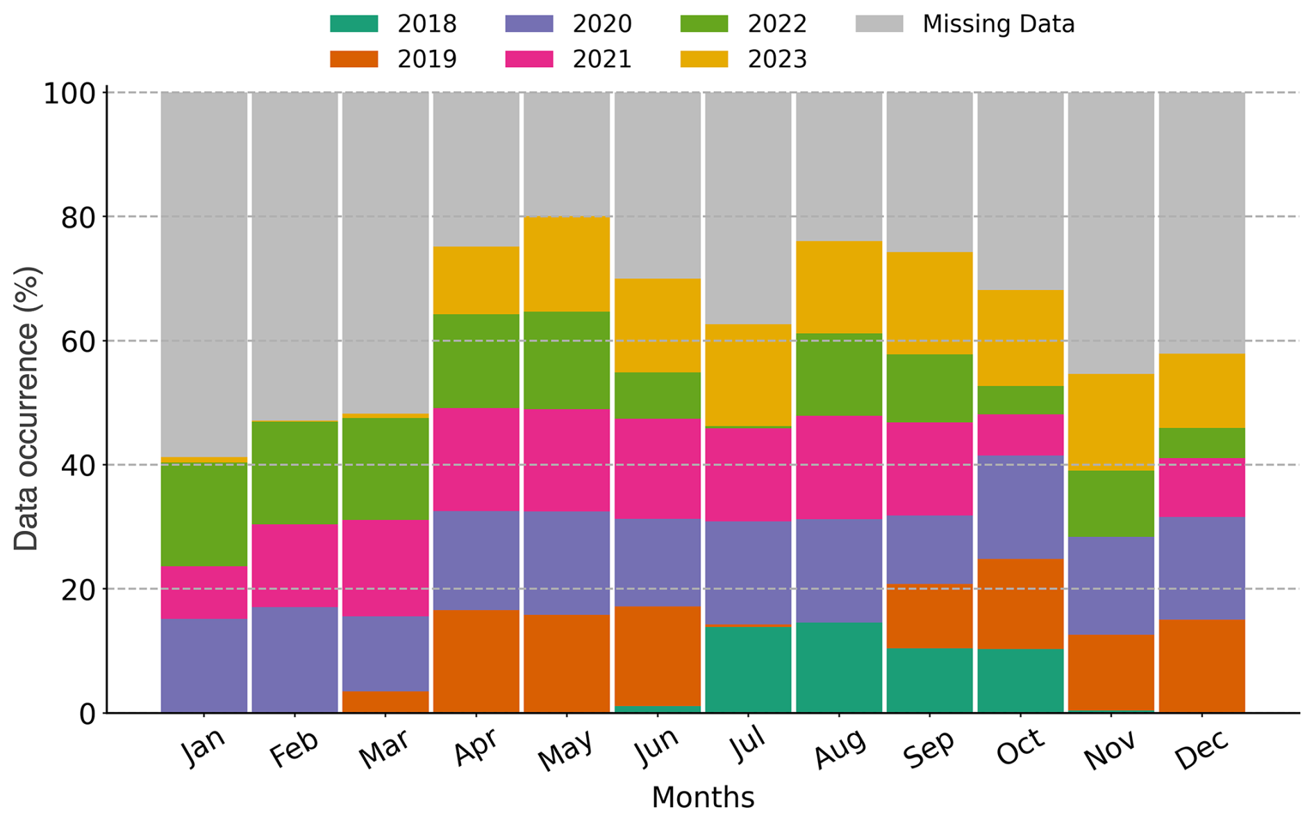
Figure 1 High-level Cloudnet post-processed data availability per month at the AGORA ACTRIS-CCRES station. This dataset represents more than half a decade of synergic ground-based measurements at this station. Each color represents the data availability for different years.

2.2 Cloudnet products

The relevant Cloudnet products in this study include the target classification (Hogan and O'Connor, 2006) and microphysical properties retrievals, such as effective radius, and liquid and ice water content. These products are re-gridded by Cloudnet to a homogeneous time resolution of 30 s and to the radar vertical range resolution. In addition, Cloudnet applies a two-way gas and liquid attenuation correction to reflectivity, since these products can be highly affected by uncorrected radar reflectivity values. In the case of high-frequency radars, such as the RPG instruments, the reflectivity suffers a strong attenuation by liquid water and gases that needs to be corrected (Hogan et al., 2003).

The target classification product (TCP) identifies each pixel (height and time) to an atmospheric component as follows: “Clear sky”, “Aerosol”, “Insects”, “Aerosol & insect” and hydrometeors: “Droplets”, “Drizzle or rain”, “Drizzle & droplets”, “Ice”, “Ice & droplets”, “Melting ice” and “Melting & droplets”. Detailed descriptions for each product can be found in Hogan and O'Connor (2006) and Schimmel et al. (2022). However, some misclassification issues were observed for the specific case of AGORA. As an example, Fig. 2 shows the temporal evolution of TCP and attenuated backscattered for 18 April 2021. Temperature lines from ECMWF model are also plotted as illustration. Below 4 km, small attenuated backscatter values are observed (Fig. 2b), which likely correspond to atmospheric aerosols typically located within the planetary boundary layer (PBL) at our station (Bravo-Aranda et al., 2015). The TCP classify most of this pixels as “Aerosol” and “Aerosol & insect”, but between 09:00 and 18:00 UTC there are some pixels around 2 km classified as “Ice” and “Drizzle or rain” (Fig. 2a), which is very rare for this altitude in this season. This was recurrent throughout the whole analyzed period and is partly associated with uncertainties in the modeled temperature at Granada under certain conditions. Thus, a pre-processing of the data was required to identify and filter out these cases, ensuring the accuracy of the statistical results. Precipitating and non-precipitating ice clouds (classified as in Sect. 3) which mean cloud bases below 4 km a.s.l. and average cloud thicknesses below 700 m were labeled as “Not Classified”.

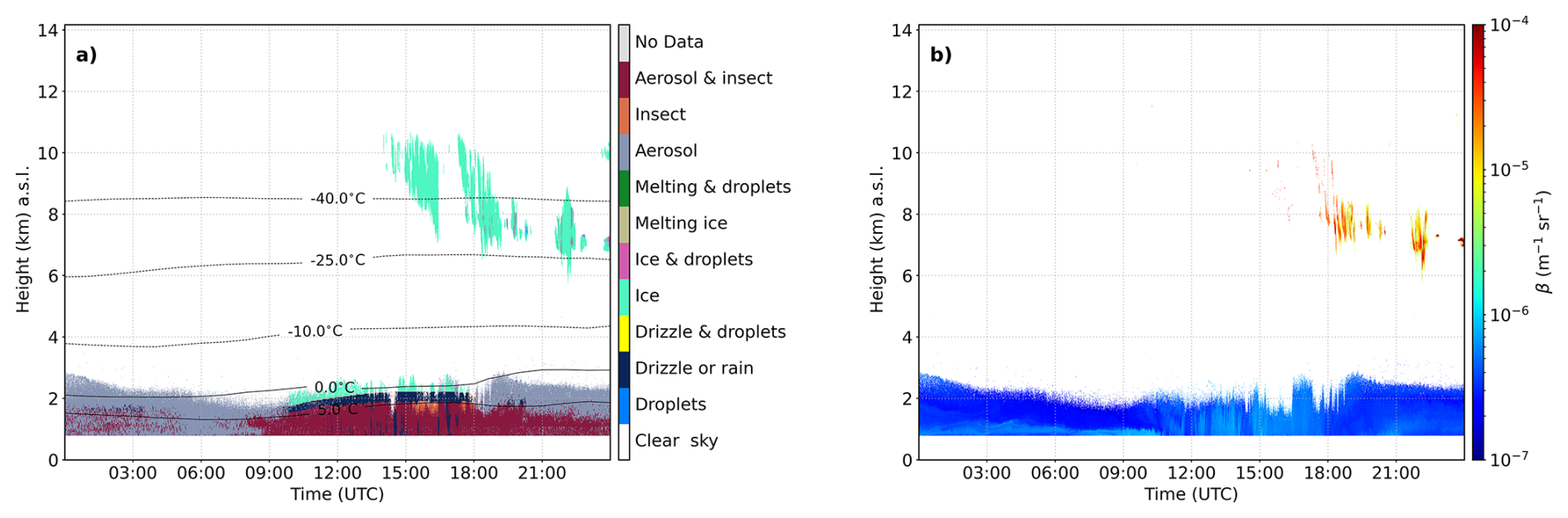
Figure 2 A case study of Cloudnet hydrometeor misclassifications; (a) Target classification product; (b) Attenuated backscattering coefficient from ceilometer, which shows no signatures of clouds in the ABL.

Liquid water content (LWC) and cloud droplet effective radius (r_liq) are retrieved at “Droplets”, “Drizzle & droplets” and “Ice & droplets” pixels. LWC is derived from LWP (from MWR), temperature and pressure (from ECMWF model), with uncertainty of 15 % (Frisch et al., 1998). Similarly, the droplet effective radius r_liq is derived for the same hydrometeors by means of the DCR reflectivity (Z) and default values of lognormal droplet size distribution (DSD), assumed by Cloudnet (Frisch et al., 2002). The uncertainty of r_liq is around 15 %, mostly associated with errors in Z (Frisch et al., 2002). For hydrometeors classified as “Ice”, ice water content (IWC) and ice effective radius r_ice are retrieved. Both derived from the Z-IWC-T (Hogan et al., 2006) and the Z-T (Griesche et al., 2019) relations, respectively. IWC uncertainty ranges from +55 % to −35 % for temperatures between −20 and −10 ^∘C, and +90 % to −47 % for temperatures below −40 ^∘C. r_ice uncertainty is around 50 %. These uncertainties highlight the challenges of accurately retrieving ice properties.

Cloud microphysical properties (i.e., radius, LWC, IWC) are computed within the cloud (i.e., skipping rain region), reducing possible contributions of rain droplets, especially relevant for the cloud LWP retrieval. Data flagged as affected by liquid water attenuation and uncertain LWP are classified as unreliable microphysical products by Cloudnet and thus they were filtered out in our analysis.

For seasonal and monthly profiles of cloud microphysical properties (in Sect. 4.3), the number of observations might be insufficient at certain heights to perform statistics. Thus, the following criteria were applied: the profile of number of observations was computed and sorted in descending order. Then, the normalized cumulative distribution was calculated, and altitude levels contributing less than 10 % to the total number of cases were excluded from the analysis.

3 Methodology

3.1 Cluster-based algorithm and cloud structure computation

The cluster-based algorithm (CBA) is a novel algorithm for hydrometeor clustering based on their proximity, distribution, and composition (i.e., the combined percentage of specific hydrometeor types relative to the total number of hydrometeor within a given cluster). The main novelty of the CBA is that it accounts for cloud volume by incorporating both cloud vertical depth and the time which cloud is observed. The time is a proxy for spatial distance due to cloud advection over the radar. This approach aims to attribute a physically meaningful representation of an individual cloud into cloud classification. Figure 3 illustrates the algorithm steps, which are described as follows:

1. Hydrometeor clustering and cloud identification

   • (a)

     Cloud Mask: A cloud mask is generated from the Cloudnet TCP.

   • (b)

     Cluster Identification: a cluster is defined as a group of connected hydrometeor identified within the cloud mask. Clusters separated by two pixels, or less, in any direction (analogous to 30 s–1 min, and 20–50 m of height) are considered a single one. For this, a pixel dilation and contraction technique is applied to all clusters in order to identify adjacent clusters (see Appendix B for further details).

   • (c)

     Cloud Criteria: Whether the cluster has more than 100 pixels, it is considered as a cloud (previously excluding Drizzle or rain pixels). Otherwise, it is “Not Classified” and is excluded from further analysis. This number of pixels was selected to avoid instrument artifacts, thus reducing the uncertainty due to pixel misclassifications.

2. Clustering classification: once a cluster is identified as a cloud, it is classified according to its phase as liquid, ice, mixed-phase, precipitating liquid, precipitating ice or precipitating mixed-phase cloud based on the following criteria. It should be noted that the Cloudnet TCP does not distinguish between snow and ice particles. Therefore, in this study, precipitation refers exclusively to liquid precipitation. This assumption is justified because snowfall is not observed at our site. The thresholds below were empirically determined after a comprehensive evaluation through multiple case studies.

   • (a)

     Liquid criteria: The percentage of “Droplets and drizzle” plus the percentage of “Droplets” is greater than 70 %, i.e. P(Droplets and drizzle) + P(Droplets) > 70 %.

   • (b)

     Ice criteria: Cluster is not classified as a liquid cloud and either “Ice” is greater than 90 %, i.e. P(Ice) >90 % or the percentage of “Droplets” plus “Ice & droplets” is less than 10 %, i.e. P(Droplets) + P(Ice & droplets) <10 %.

   • (c)

     Mixed-phase criteria: If the cluster is not classified as liquid or ice cloud, then it is classified as a mixed-phase cloud

   • (d)

     Rain criteria: Clouds with more than 10 pixels of “Drizzle or rain” are classified as precipitating clouds.

3. Cloud structure computation

   • (a)

     Cloud base height (CBH) definition: they are the first cloud pixels detected by the ceilometer for all non-precipitating clouds. For precipitating liquid clouds, CBH is the first cloudy pixel above “Drizzle & rain” layer. For ice and mixed-phase precipitating clouds, it is the first pixels within the melting layer. Hydrometeors below the melting layer are excluded from the cluster to prevent underestimation of CBH.

   • (b)

     Cloud top height (CTH) definition: last cloud pixels detected by the CDR. It is not valid when radar LWP is greater than 0.9 kg m⁻². In this case, CTH is filtered because liquid water attenuation can mask cloud tops, underestimating CTH and cloud thickness.

   • (c)

     Cloud thickness definition: the difference between cloud base and top height pixels.

4. Multi-layer classification

   • (a)

     Multi-layer criteria: For cloudy periods, the time interval where two or more clouds exists is classified as multi-layer. Otherwise, it is classified as a single-layer type.

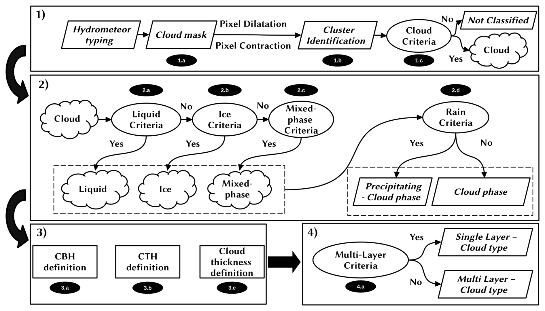
Figure 3 Flowchart of the cluster-based algorithm (CBA). Details of each step are provided in the text. Pixel dilatation and pixel contraction method is explained in Appendix B.

Multi-layer clouds prevent a proper retrieval of the LWC (Shupe et al., 2015), since accurate profiles can not be obtained. First, lidar data are required to detect small droplets at the cloud base; however, its signal cannot penetrate to higher layers due to total attenuation. Second, CDR signals in upper layers is weakened by attenuation from lower layers and is insensitive to small particles. This makes it challenging to identify “Droplets” and “Ice & droplets” pixels, increasing uncertainty in cloud structure (e.g., cloud base and top) and microphysical retrievals (Nomokonova et al., 2019; Shupe et al., 2015). Therefore, the following analyses are focused only on single-layer clouds, since their physical properties can be accurately retrieved.

3.2 Cloud typing assessment

A comparison between CBA and the profile-based algorithm (PBA) (see Appendix A for a description) was conducted to evaluate their applicability on cloud statistics. Figure 4 presents results of the comparison on 6 May 2023 where a mixed phase cloud structure is observed between 5 and 7 km a.s.l. (Fig. 4a). The CBA and PBA classifications are shown in Fig. 4b and c. As it can be seen, the PBA fragments the cloud into ice and mixed-phase multiple times whereas CBA classifies the whole cloud as mixed-phase one, preserving the homogeneity of the cloud structure.

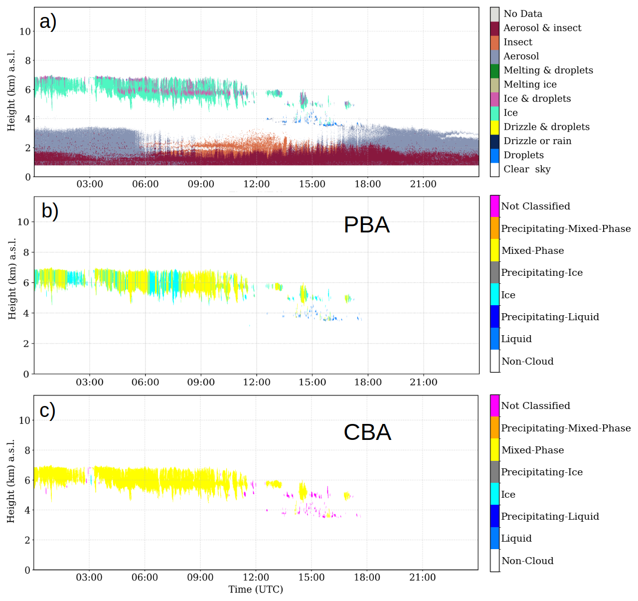
Figure 4 Comparison of cloud typing from different cloud classification algorithms at the AGORA station, on 6 May 2023; (a) TCP from Cloudnet, indicating a clear single layer of Mixed-Phase cloud (b) PBA cloud typing, showing an inhomogeneous cloud classification. (c) CBA cloud typing, showing an homogeneous cloud classification.

The inhomogeneous PBA's cloud classification may result in assigning similar cloud properties to different cloud types. As can be clearly seen in Fig. 4b, both ice and mixed phase clouds will have similar daily cloud occurrence and average CBH and thickness. However, this is a consequence of the classification algorithm, which could affect further analysis of cloud type properties, leading to unproper conclusions.

Pearson correlation coefficients of daily occurrence, daily average CBH, cloud thickness, and IWP are calculated between ice and mixed-phase clouds for CBA and PBA to assess the classification algorithm's impact on cloud property statistics. The PBA correlations for daily occurrence, CBH, thickness, and IWP averages are 39 %, 80 %, 84 % and 70 %, respectively, and for CBA are 8 %, 56 %, 1.1 %, and 1 %, respectively. It shows much larger correlations for the PBA, indicating that the CBA can better distinguish different cloud types by providing a more physically meaningful representation of individual clouds. Additionaly, Fig. 5 shows the monthly median cloud thickness for ice and mixed-phase clouds for CBA and PBA (Fig. 5a and b, respectively). Despite the large variability in both approaches, the PBA clearly shows the same seasonal pattern (highly correlated) between ice and mixed clouds. This reveals that CBA accounts for cloud properties variability among different cloud types and it is especially evident in regions with marked seasonalityl. In our case, temperature, relative humidity, and aerosol loading present a strong seasonal behavior (Bedoya-Velásquez et al., 2019; Pérez-Ramírez et al., 2012; Lyamani et al., 2010), which influences cloud formation, and different seasonal patterns in cloud thickness are expected since ice and mixed-phase clouds are formed through different physical processes. Pure ice clouds are formed by direct vapor-to-ice or homogeneous freezing at low temperatures (Lüttmer et al., 2025; Knopf and Alpert, 2023), whereas mixed-phase clouds rely on supercooled liquid plus INP-mediated freezing, Wegener-Bergeron-Findeisen (WBF) processes and turbulence (Maciel et al., 2024; Mioche et al., 2017; Korolev and Milbrandt, 2022; Huang et al., 2021). These findings underscore how these two algorithms associate different cloud types, which can impact the statistical analysis of cloud properties. Moreover, the CBA is a robust and accurate method for determining cloud macrophysics, presenting a coherent cloud phase representation without suppressing cloud variability.

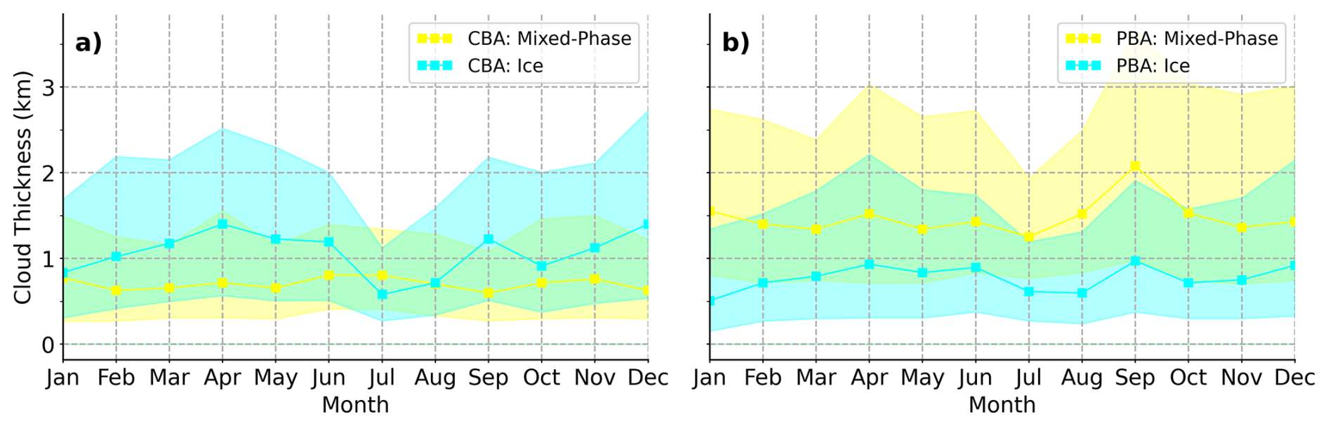
Figure 5 Comparison of monthly median cloud thickness between ice (yellow) and mixed-phase (blue) clouds for CBA (a), and for PBA (b). The interquartile range is denoted by the shaded area.

A sensitivity analysis of cloud property statistics (i.e., CBH, cloud thickness, LWP, IWP) against the classification thresholds defined in Sect. 3 can be found in Appendix C. The analysis indicates that the CBA is robust to threshold perturbations, showing small differences in cloud properties and preserving its seasonal patterns. This confirms that the proposed CBA and its conclusions are not sensitive to the particular choice of thresholds within physically meaningful ranges. In this light, the new approach shows a promising classification method and will be employed in this study.

4 Results and discussion

4.1 Cloud frequency annual variability

Figure 6a presents the monthly cloud occurrence frequency at AGORA station (i.e. the number of occurrence of a particular cloud, divided by the total number of observations at each month), for different sky conditions, i.e. Single-layer clouds, Multi-layer clouds, Clear-sky (when there is no clouds), and Not classified (as defined in Sect. 3.1). The analyzed dataset covers the period from 2018 to 2023, and reveal a distinct seasonal pattern in cloud cover and clear sky occurrences. Clear sky conditions (green line) dominate most of the year, being most frequent in summer, with maximum in July and August (>80 %), and reaching their lowest values in March and April (40 %), when cloudy skies are predominant. This pattern highlights the predominance of clear skies during the warmer months and increased cloudiness during the colder months. The meteorological conditions with very dry summers and relatively humid springs and winters can support these observations. Single-layer (blue line) and multi-layer clouds (orange line) exhibit very similar values with a relatively weak seasonal pattern throughout the year showing maxima in spring and minima in the summer months. Multi-layer clouds present a slightly more pronounced seasonal variation than single-layer clouds, with higher occurrence in spring (35 % for multi-layer and 25 % for single-layer clouds in April) and lower occurrence in summer (3 % for multi-layer versus 9 % for single-layer clouds in July).

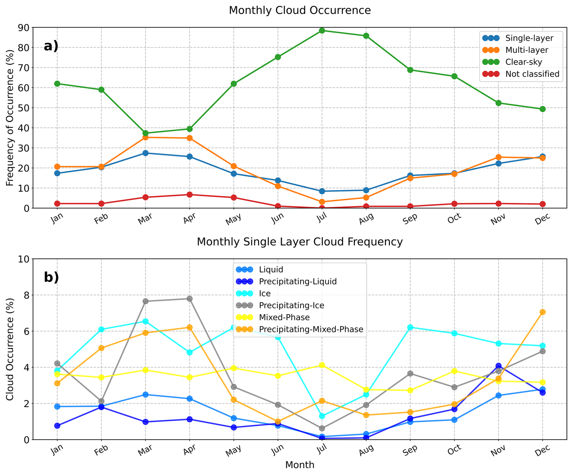
Figure 6 (a) Monthly frequency of occurrence for single layer clouds (blue), multi-layer clouds (orange), clear sky (green) and noise (red). (b) Inter-annual frequency of occurrence for single layer clouds for different cloud types (see Sect. 3.1). Each cloud type is indicated at the legend box.

As noted in Sect. 3, the analysis focuses on single-layer clouds. Figure 6b presents their monthly occurrence by cloud type. Percentages are given with respect to the total number of observations at each month.

Liquid clouds occur infrequently (<3 %), and are almost absent in July and August. Precipitating liquid clouds contribute less than 2 % annually, with a slight maximum in November (∼ 4%). Their occurrence maximum occurs during autumn, exceeding that of non-precipitating liquid clouds, although the seasonal contrast remains weak.

Throughout the year, ice cloud occurrence is varying around 5 % and 7 %, except in July and August when values sharply drop below 3 %. It exhibits a clear seasonal pattern, with a small presence of ice clouds in summer. Precipitating ice clouds have maximum frequency in spring (8 %) and winter (5 %). The frequency of occurrence sharply decrease in May, reaching a minimum in July with less than 1 %. These results reveal a strong seasonality for the occurrence of ice clouds.

Mixed-phase clouds exhibit a consistent occurrence around 3 % and 4 % throughout the year. Its steady frequency indicates an absence of seasonal pattern. Precipitating mixed-phase clouds show maximum values in April (6 %) and December (7 %). Their minimum is also reached in summer, being less than 2 % in June and August. This indicates a pronounced seasonality for precipitation from mixed-phase clouds, with maxima exceeding non-precipitating mixed-phase clouds in spring and winter.

Therefore, we can conclude that at the AGORA station cloud frequency reaches a minimum during summer when atmospheric stability is pronounced (Bedoya-Velásquez et al., 2019), also affecting precipitation. Strong seasonal patterns with maxima in spring and fall and minima in summer are observed for all types of precipitating clouds, whereas ice clouds are the only non-precipitating clouds with a pronounced seasonality. Ice clouds (both precipitating and non-precipitating) are the most frequent, followed by the mixed-phase type. Moreover, precipitating clouds have considerable presence of ice, i.e. precipitating ice and precipitating mixed-phase clouds.

4.2 Seasonal analysis of cloud macrophysical properties

The study of cloud macrophysical properties implies the analysis of CBH, CTH, and cloud thickness. The seasonal evolutions of these properties are displayed in Fig. 7, while the median values of CBH and cloud thickness are shown in Table 2. Figure 7 shows the seasonal vertical distributions of CBH, CTH and cloud thickness, for different cloud types (liquid, ice and mixed-phase) differentiating between precipitating and non-precipitating clouds in each panel. Dashed lines in the distribution represent the 25/50/75th percentiles. Note that for homogenization data are shown in the range 0–12 km, except for cloud thickness in liquid clouds where a zoom for the first kilometer is made for clear visualization. For the seasonal analysis, climatological definitions were used: spring (March, April, May), summer (June, July, August), fall (September, October and November) and winter (December, January and February).

Liquid clouds generally exhibit low CBH, except in summer, which shows a distribution approximately 500 m higher than in other seasons. The median CBH in summer is 2.09 km, while in the other seasons, it ranges from 1.31 km in winter to 1.49 km in spring, as shown in Table 2. The CTH follows the same seasonal pattern as CBH but with slightly higher values. Consequently, a narrow distribution of cloud thickness is observed (Fig. 7c – zoomed for better visualization). Precipitating liquid clouds have median CBHs below 1 km in all seasons except summer, which has a median CBH of 1.25 km (see Table 2). These clouds exhibit a narrower distribution of both CBH and CTH compared to liquid clouds. However, they show greater cloud thickness, nearly twice that of liquid clouds during summer and winter, as shown in Table 2.

Ice clouds are found at much higher altitudes, with CBH median values ranging from 7.24 km in winter to 8.14 km in fall (see Table 2). These values indicate a well-defined vertical structure with minimal seasonal variation. A similar pattern is observed for CTH, which remains consistently high, exceeding 9 km (Fig. 7e). Figure 7f shows that some ice clouds exceed 3 km in thickness. However, their median width remains around 1 km, with a maximum of 1.27 km in spring, as shown in Table 2. Precipitating ice clouds exhibit lower CBH, with median values of 1.61 km in winter and spring, increasing to 2.83 km in fall and 3.55 km in summer (see Table 2). This seasonal variation suggests a pronounced dependence on atmospheric conditions. Figure 7f shows that these precipitating ice clouds have a broader distribution of cloud thickness, with median values ranging from 3.25 km in winter to 4.14 km in summer, indicating thicker clouds in warmer months. Precipitating ice-clouds present a much lower CBH compared to non-precipitating ones, consequently leading to much higher median thickness for all seasons.

Mixed-phase clouds have CBHs at mid-level altitudes, with distributions varying significantly across seasons (Fig. 7g). However, the median CBH shows moderate variation, ranging from 4.77 km in winter to 6.50 km in summer, as shown in Table 2. A similar seasonal pattern is observed for CTH. Despite this variability, the median cloud thickness remains relatively stable at 0.68 km, except in summer, when it slightly increases up to 0.77 km. Precipitating mixed-phase clouds exhibit lower CBHs, with median values below 2 km in all seasons except summer, where it reaches 4.47 km (see Table 2). A similar pattern is observed for CTH, which shows increased values in summer. In terms of cloud thickness, the median is below 2 km with slightly higher values in summer (see Table 2).

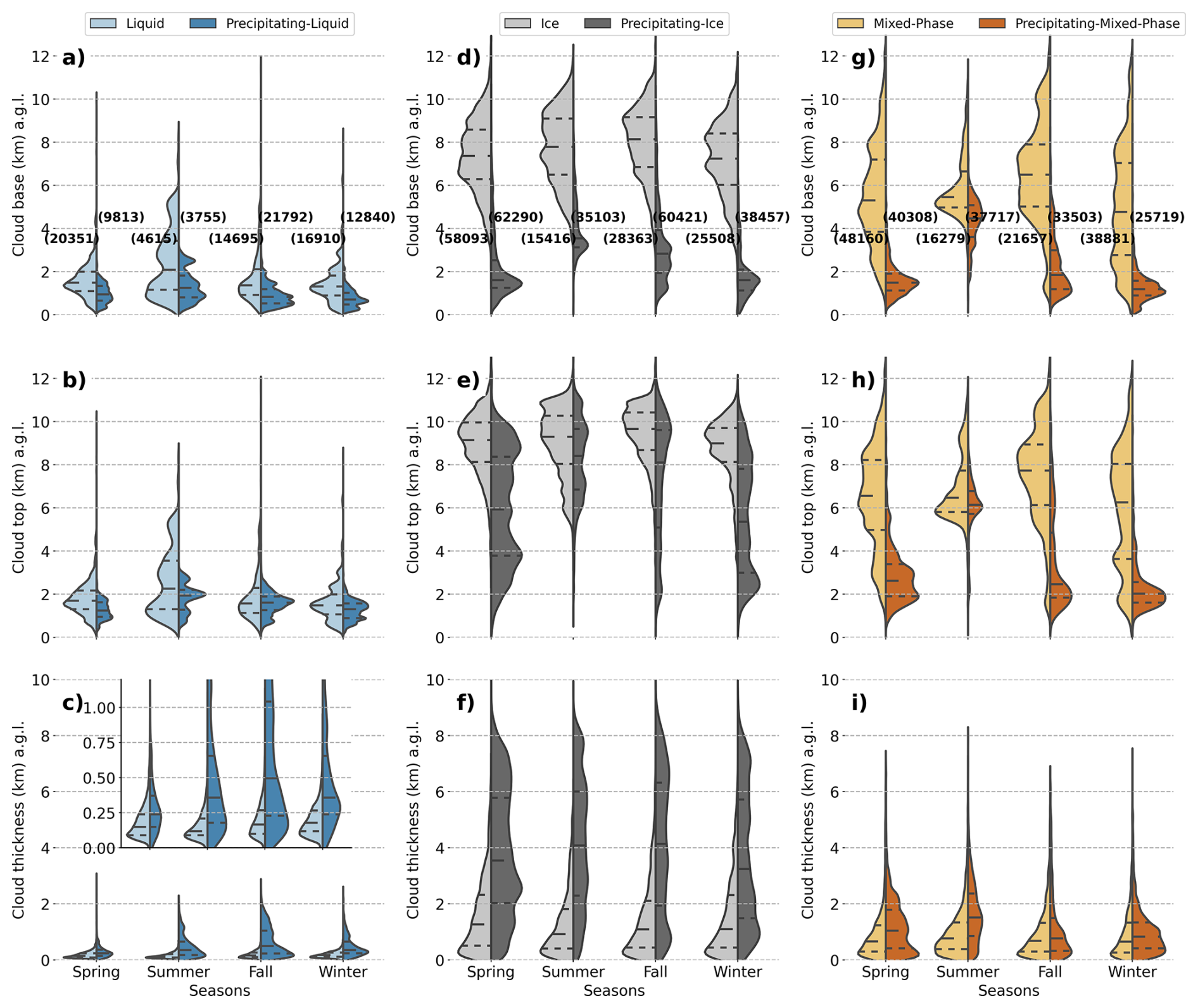
Figure 7 Seasonal distribution of cloud base height (a, d, g), top height (b, e, h), and thickness (c, f, i) for different cloud types: liquid (a, b, c), ice (d, e, f), and mixed phases (g, h, i). Each color represents a cloud type, with liquid clouds in blue, ice clouds in gray, and mixed-phase clouds in orange. Light colors represent non-precipitating clouds, and dark colors represent precipitating clouds (see legend on top of the figure). The values in parentheses represent the number of measurements for each cloud type. Dashed lines within distributions contour indicates $\mathrm{25}/\mathrm{50}/\mathrm{75}$th percentiles.

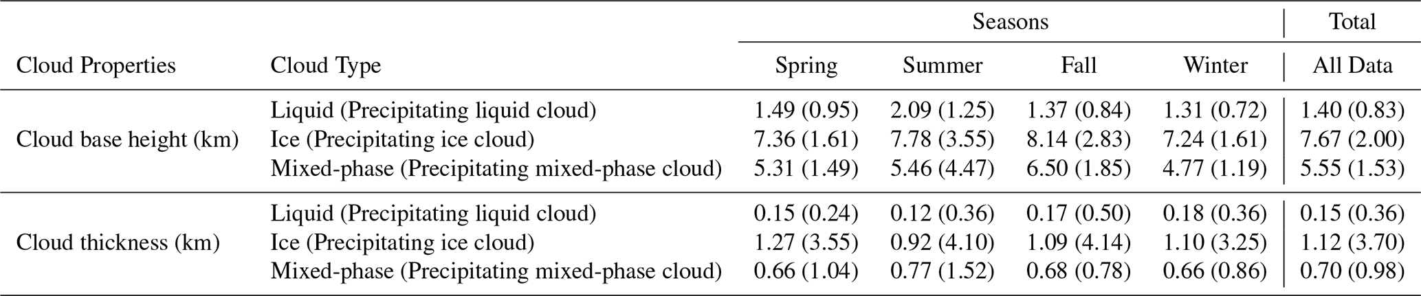
Table 2 shows that precipitating ice clouds exhibit the greatest median cloud thickness (3.7 km), followed by ice clouds (1.12 km), precipitating mixed-phase clouds (0.98 km), mixed-phase clouds (0.7 km), precipitating liquid clouds (0.36 km), and liquid clouds (0.15 km). Ice clouds have the highest cloud base height (CBH) at 7.67 km, followed by mixed-phase clouds (5.55 km), whereas precipitating liquid clouds exhibit the lowest CBH. In general, precipitating clouds have significantly lower CBHs than their non-precipitating counterparts and exhibit a stronger seasonal variation, with higher bases in summer.

Despite the attenuation correction applied in Cloudnet post-processing and the LWP filter for values exceeding 0.9 kg m⁻², which only accounted for 1 % of cases, precipitating clouds still exhibit the largest variability in cloud thickness. This highlights their high heterogeneity and may also suggest that attenuation effects are not fully corrected. Liquid water attenuation is major challenge in cloud radar data that needs to be carefully addressed. Additionally, CBH is sometimes determined by “Drizzle & Droplets” pixels, which may already correspond to precipitation, leading to a potential underestimation of cloud base height. This effect is more pronounced in marine environments (Roschke et al., 2024), though it is less relevant for the AGORA station.

Table 2 Cloud macrophysical properties per season and cloud type. Median values of cloud base height and cloud thickness are shown. The values in parentheses correspond to precipitating clouds. An additional column presents the median values for the total dataset.

4.3 Cloud microphysical properties

In this section we investigate the inter-annual variability of microphysical retrievals for each category of single-layer clouds detected at the AGORA station. Liquid water content (LWC) and droplet effective radius (r_liq) were evaluated for liquid and mixed-phase clouds, while ice water content (IWC) and ice effective radius (r_ice) were evaluated for ice and mixed-phase clouds. The analysis was performed for the precipitating and non-precipitating cases.

4.3.1 Liquid clouds

Interannual variability of LWC profiles and LWP for liquid clouds is illustrated in Fig. 8a. The figure presents seasonal and monthly median profiles of LWC (top-left and top-right panels, respectively), and monthly LWP statistics (bottom panel). As seen in the top-left panel, LWC in general shows a roughly constant value over 60 mg m⁻³ in winter and spring, in addition to a slight increase with height observed in summer and fall. The nearly constant LWC with height is consistent with prior in-situ studies of stratocumulus and shallow liquid clouds, which report sub-adiabatic vertical profiles due to entrainment and mixing of dry air (Pawlowska et al., 2000; Gerber, 1996). By contrast, the increase with height agrees with previous studies reporting quasi-adiabatic growth due to continuous condensation in ascending moist air, particularly in stratocumulus and shallow cumulus under low entrainment conditions (Brenguier et al., 2003; Albrecht et al., 1988). In summer, clouds located between 3 and 4 km exhibit LWC values around 480 mg m⁻³, primarily associated with a maximum observed in August (see top-right panel, Fig. 8a). Additionally, summer is the only season in which liquid water is detected above 3 km. For the rest of the seasons, more than 75 % of cloud tops are located below this altitude (see Fig. 7). In winter and spring, LWC values exceeding 300 mg m⁻³ are observed between January to May associated to specific events. These peaks do not significantly influence the seasonal statistics, as observed in the seasonal profile (left panel, Fig. 8a). Spring also exhibits the largest variability near 600 m, due to elevated LWC in April. In contrast, fall does not show similarly high LWC values in any month. In general, the LWP does not show a clear seasonal pattern, although its variability is highest during spring. This is also observed in the monthly LWP, which presents low variability with monthly values close to the annual median of 11.5 g m⁻².

Figure 8b presents the same analysis as Fig. 8a, but for precipitating liquid clouds. As seen in the top-left panel, LWC increases approximately linearly with height, except during spring. The deeper thickness of these clouds, compared to non-precipitating ones, allows for the observation of a clear decrease in LWC near the surface. This is in agreement with previous studies showing that rain formation depletes water at lower altitudes, while active condensation above sustains higher LWC values (Gerber, 1996; Wood, 2005). In spring, a maximum of 270 mg m⁻³ occurs near 450 m, followed by relatively constant values around 100 mg m⁻³ up to approximately 1.7 km, which is quite different from the patterns observed in other seasons. This peak is primarily associated with high LWC values in April (see top-right panel), likely due to the presence of rain droplets. Spring is season with higher occurrence of precipitating clouds, and it is often difficult to distinguish between “Drizzle & droplets” and “Drizzle or rain” pixels near the cloud base. As a result, some “Drizzle & droplets” pixels within the cloud may be misclassified, potentially leading to an overestimation of LWC in the lower levels. In contrast, summer and fall exhibit similar vertical profiles, extending up to 2 km, where LWC values reach approximately 250 and 270 mg m⁻³, respectively. The LWC observed at 2.6 km in summer is primarily due to elevated values in June, as indicated in the top-right panel. Winter also shows a similar profile up to 1.5 km, but with even higher LWC values, mainly driven by observations in January and February. The bottom panel further shows that January has the highest LWP, along with the biggest variability. Although annual median is 40.0 g m⁻², monthly values can be quite different.

The spatial-temporal distribution of r_liq for liquid clouds is shown in Fig. 8c. The figure shows seasonal (top-left) and monthly (top-right) median profiles of r_liq, with the bottom panel presenting general monthly statistics. The top-left panel shows minimal seasonal variation in the vertical profiles, with nearly constant r_liq with height. This trend is also seen in the monthly profiles (top-right panel), where values mostly range around 4 and 6 µm. Besides the fact droplets larger than 6 µm is found above 5 km in August, and below 600 m in winter, the variability is so high that in general, droplets size barely changes. Similar behavior was observed by previous studies (E. Gerber et al., 2008; Gao et al., 2021; Gerber, 1996; Pawlowska et al., 2000; Brenguier et al., 2003), which attribute this behavior to limited condensation growth under sub-adiabatic and mixing-influenced conditions. Additionally, monthly r_liq are generally close to the annual median of 5.3 µm, except in July (4.4 µm), where a minimum is observed.

For precipitating liquid clouds, the seasonal profiles of r_liq in the top-left panel of Fig. 8d show a clear separation between profiles. During summer and fall, it exhibits an increase with height up to a certain altitude, beyond which it begins to decrease, whereas in winter and spring, it remains nearly constant throughout the vertical profile. For summer and fall, this behavior are consistent to previous studies showing that droplet size grows with height in developing drizzle–precipitating conditions until the onset of substantial coalescence and fallout (Chen et al., 2008). On the other hand, winter and spring are consistent with observations under light drizzle conditions, where coalescence is active but the vertical gradient of droplet size weakens as fallout offsets further growth (Chen et al., 2008). Fall exhibits the largest droplet sizes throughout the profile, while summer shows r_liq values relatively close to those of spring below 1 km and to winter above 1.5 km. Except for summer, where droplet sizes increase with height up to 2 km, other seasons show an increase in r_liq up to approximately 1 km, followed by stabilization or a slight decrease with altitude. In fall, the peak r_liq of 10 µm is primarily attributed to large droplet sizes observed in October and November (see top-right panel). Similarly, the winter peak of 8 µm is mainly driven by January observations. This is supported by the bottom panel, which shows r_liq values of 9.5 µm in November and 8.5 µm in January. For the other seasons, however, it is difficult to clearly associate the seasonal medians with specific monthly patterns. Although the annual median droplet size is 7.7 µm, pronounced monthly variability is observed, with fall exhibiting the largest droplet sizes and summer the smallest. The minimum in July, also observed for liquid clouds, may be associated with enhanced Saharan dust loading, although further investigation is required.

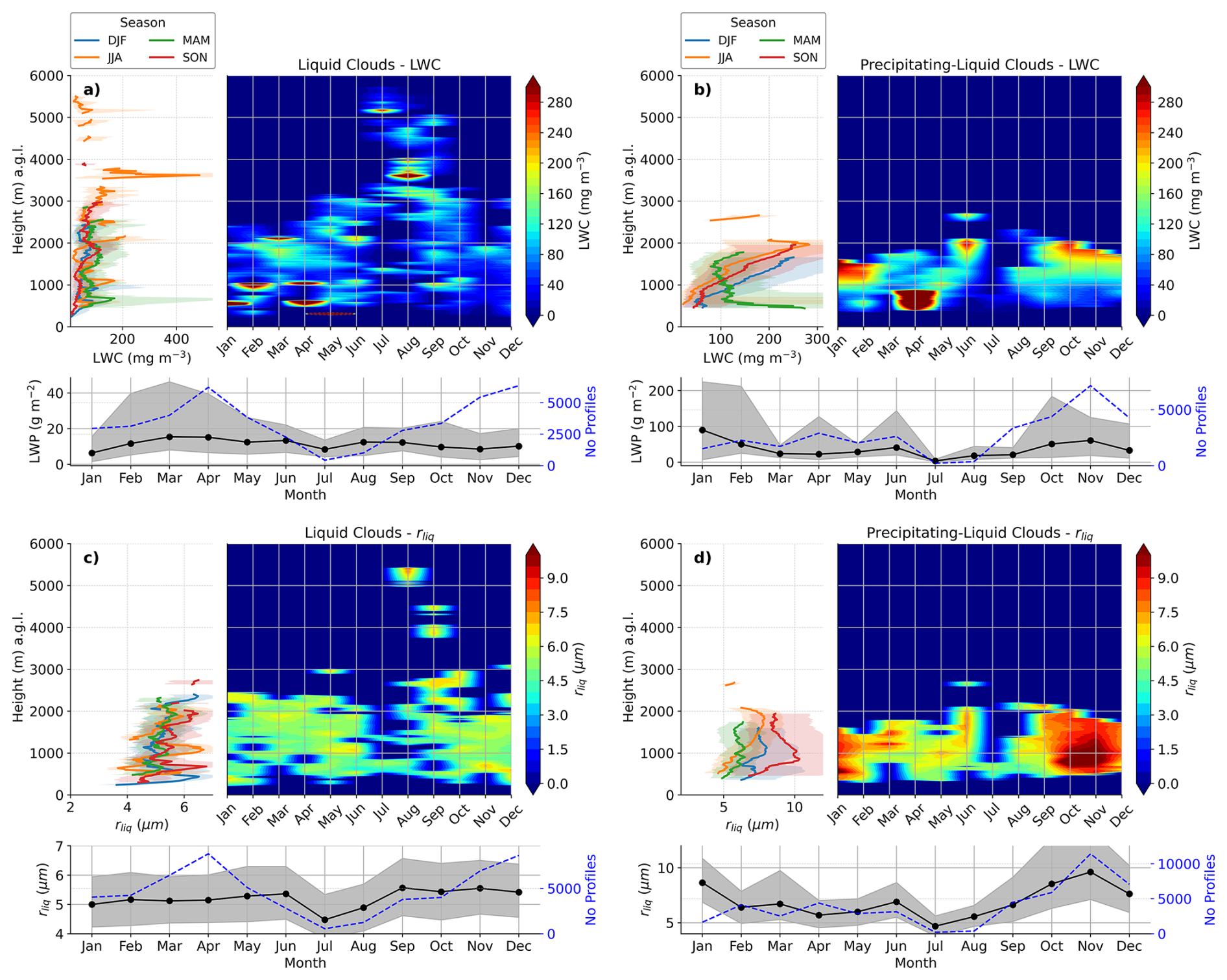
Figure 8 Seasonal and monthly profiles of microphysical properties for liquid clouds and precipitating liquid clouds. For liquid clouds, (a) presents median vertical profiles of LWC by season (a, c), by month (b, d), and monthly median LWP (c, d). (c) shows vertical profiles of droplet effective radius (r_liq) by season (a, c), by month (b, d), and monthly r_liq statistics in the bottom panel. (b) and (d) present the same as (a) and (c), respectively, but for precipitating liquid clouds. Shaded areas denote the interquartile range, and the blue lines in bottom panels indicate the number of profiles used in each month.

Considering the observed results, precipitating liquid clouds exhibit higher LWP and r_liq compared to non-precipitating liquid clouds, as expected (Li et al., 2025). Median LWP and r_liq for precipitating clouds are 36.0 g m⁻² and 7.7 µm, respectively, while for liquid clouds they are 11.5 g m⁻² and 5.3 µm. It is consistent with the progression of microphysical growth toward precipitation, where larger LWP indicate deeper clouds (see Table 2), providing more mass for droplets to grow through condensation and coalescence (e.g., Pruppacher and Klett, 2010; Freud and Rosenfeld, 2012). Next, liquid clouds show less seasonal differences, with LWC extending to higher altitudes in summer, larger LWP variability in spring, and the smallest r_liq values in summer. In contrast, precipitating liquid clouds present seasonally distinct LWC profiles, with higher values in winter, highest LWP in January, and the largest droplet sizes in fall. Overall, the LWC and r_liq in precipitating clouds are substantially more variable.

4.3.2 Mixed-phase clouds

Seasonal and monthly statistics of LWC and LWP in mixed-phase clouds are displayed in Fig. 9a. This figure shows the same as Fig. 8a, but for mixed-phase clouds. As shown in the top-left panel, LWC is roughly between 50–100 mg m⁻³ below 4 km, decreasing to 10–20 mg m⁻³ above this level. Winter and spring exhibit similar LWC profiles between 2.5–3.5 km, with values around 70 mg m⁻³. Within this layer, the highest variability is found, primarily driven by enhanced values in January, February (winter), and April (spring), as indicated in the top-right panel. The winter maximum at 1 km is associated with the high occurrence of mixed-phase clouds during the Filomena and Gloria storms in January 2020 and 2021 (Buisán et al., 2022; Pérez-González et al., 2022; Marta de Alfonso et al., 2021), respectively. During these months, high presence of ice in the atmosphere was observed, and low-level “Drizzle & Droplet” pixels are occasionally mixed with ice particles, which may bias LWC due to large ice crystals presence. These pixels were not filtered out, as the presence of ice is inherent to mixed-phase clouds. Moreover, identifying the presence of large ice particles remains a significant challenge and falls beyond the scope of this study. This is reflected in the large LWP variability observed in January (bottom panel). Nonetheless, monthly median LWP remains relatively stable throughout the year, with values close to the annual median of 8.9 g m⁻².

Similarly, Fig. 9b shows the same Fig. 9a, but for IWC and IWP. The top-left panel shows that IWC is predominantly observed above 4 km, positioned slightly above the LWC layer, which is mostly confined below this altitude. This behavior is primarily due liquid-to-ice phase transition. This process is driven by processes such as the Bergeron–Findeisen mechanism, in which ice crystals grow at the expense of supercooled liquid water (Korolev et al., 2017). Next, summer and fall exhibit similar trend up to 7 km. Above this level, IWC in summer increases to a maximum of 20 mg m⁻³ at 8 km before decreasing at a similar rate to fall, which have a maximum around 15 mg m⁻³. According to the top-right panel, the summer maximum is primarily due to elevated values in June and August, while the fall maximum is driven by October observations. Winter and spring also display comparable trends, except between 4–6 km, where they have the largest differences. The winter maximum at 6.4 km of 15 mg m⁻³ is mainly driven by clouds formed in January and February, while the rapid increase in IWC around 4.5 km during spring is largely driven by clouds in April. The bottom panel shows greater interquartile variability in IWP compared to LWP across most months, except January. However, the monthly median values are quite stable around the annual median of 3.5 g m⁻².

Figure 9c presents the same as Fig. 8c, but for mixed-phase clouds. The top-left panel shows an initial increase in droplet size with altitude, followed by a decrease at higher levels. According to Korolev and Mazin (2003) and Korolev et al. (2017), supercooled droplets are expected in the lower part of mixed-phase clouds, typically at temperatures above −10 °C, where ice nucleation is limited. This is agreement with our observations, showing an increase in droplet sizes up to approximately 4 km, coinciding with low IWC. Above this altitude, the Bergeron–Findeisen process leads to droplet evaporation, while colder temperatures enhance ice nucleation efficiency, resulting in a decrease in droplet size. In winter and spring, r_liq increases up to approximately 13.5 µm at 4 km before decreasing with height. These maxima are primarily associated with January–April, respectively, as shown in the top-right panel. In fall, r_liq increases with altitude, reaching up to 13 µm at 6.6 km, whereas in summer, it starts around 5 km, with maximum of 15.5 µm, and decreases with height. These maxima are mainly driven by observations in September–October (fall) and June–August (summer). The bottom panel indicates the monthly medians deviate less than 2 µm from the annual median of 10.8 µm, with largest deviation in summer, when r_liq reaches 12.4 µm in July.

The statistics of ice effective radius (r_ice) are presented in Fig. 9d. The top-left panel of this figure shows a nearly steady size up to 6 km, followed by a decrease in all seasons. This occurs because ice particles may remain nearly constant in size or grow through vapor deposition and rimming up to a certain altitude. However, above that, processes such as reduced water vapor availability, fragmentation, and sedimentation lead to a decrease in particle size (Korolev et al., 2017). Although the overall profiles are similar, summer and fall exhibit slightly larger sizes above 7 km. At the first 6 km, r_ice is roughly constant, varying between 42 and 48 µm. Above this altitude, particle sizes gradually decrease, reaching values between 30–40 µm. This pattern is also evident in the monthly profiles shown in the top-right panel by the positive gradient towards the ground. The bottom panel shows greater interquartile variability and monthly median deviations from the annual median compared to r_liq. The annual median is 44.7 µm, with maximum difference observed in February (∼ 4 µm). Additionally, r_ice is slightly larger in summer, particularly in July. A similar pattern was observed for r_liq.

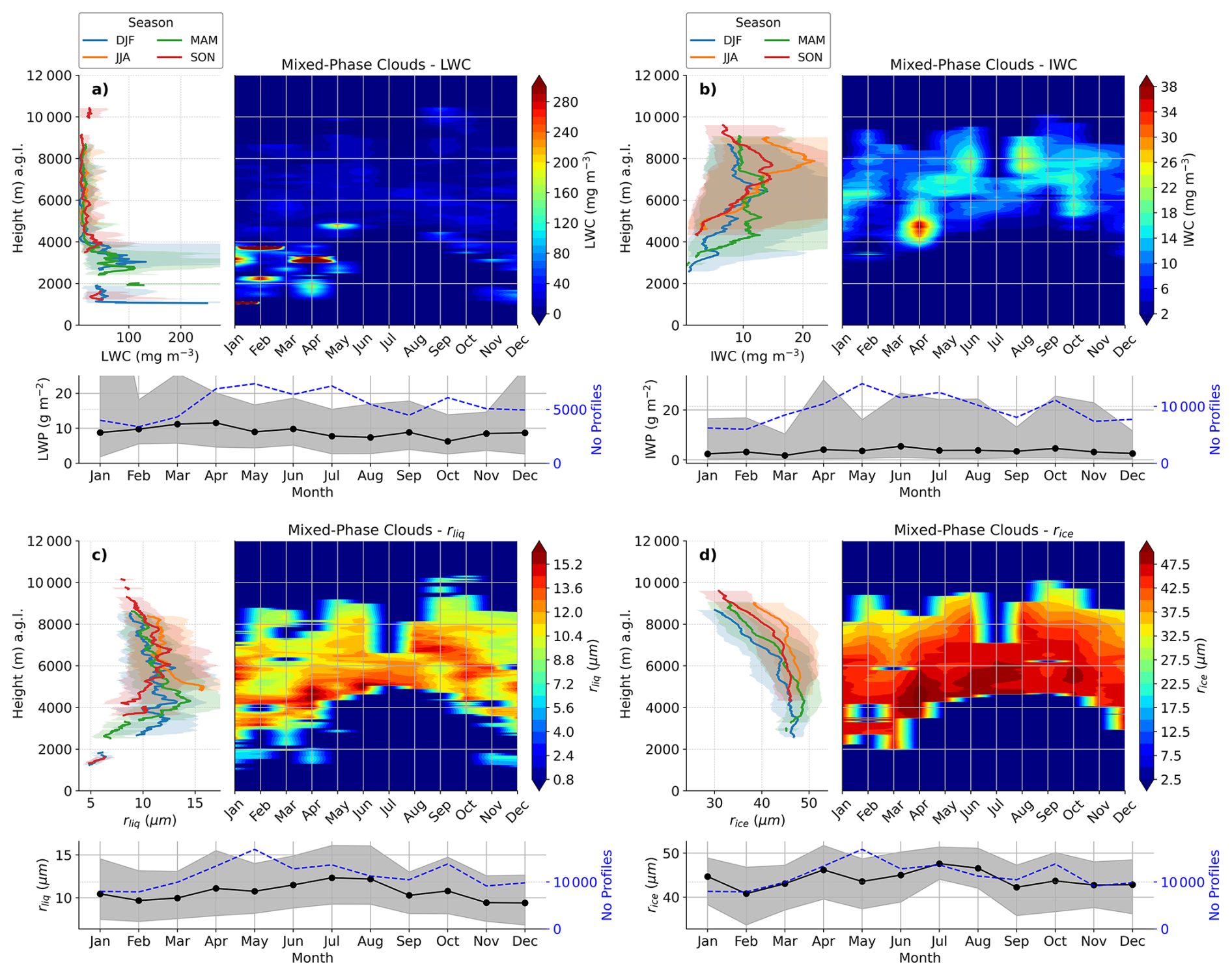
Figure 9 Seasonal and monthly profiles of microphysical properties for mixed-phase clouds. (a) presents median vertical profiles of LWC by season (a, c), by month (b, d), and monthly median LWP (c, d). (b) shows the same as (a), but for IWC and IWP, respectively. (c) shows vertical profiles of droplet effective radius (r_liq) by season (a, c), by month (b, d), and monthly r_liq statistics (c, d). (d) shows the same as (c), but for r_ice. Shaded areas denote the interquartile range, and the blue lines in bottom panels indicate the number of profiles used in each month.

The analysis shows that mixed-phase clouds exhibit higher LWC than IWC, and the variability in LWC is notably smaller compared to IWC. Additionally, LWC is predominant in the lower part of the cloud, while IWC is predominant in the upper part of the cloud. This is in agreement with the liquid depletion observed by Korolev and Field (2008) in mixed-phase clouds. Regarding particle sizes, the ice effective radius (r_ice) is significantly larger than the liquid effective radius (r_liq), and also shows greater variability.

Figure 10 shows the same analyses than in Fig. 9, but for precipitating mixed-phase clouds. As illustrated in Fig. 10a, these clouds exhibit distinct LWC profiles across seasons. For the lowest 2.5 km, fall and winter exhibit similar LWC profiles, with values ranging from 100 to 150 mg m⁻³. Spring shows the highest LWC within this layer, with two maximums of 300 mg m⁻³ at approximately 900 m and 1.8 km. These maxima are associated with observations in March and April, as shown in the top-right panel. Although summer lacks sufficient data below 4 km, the monthly analysis indicates high LWC around 2.4 km in June. Above 2.5 km, LWC decreases significantly in winter and spring, remaining around 25 mg m⁻³, roughly 50 mg m⁻³ lower than fall, up to 4.2 km. Above this level, only fall and summer maintain detectable LWC, typically below 40 mg m⁻³. The bottom panel shows considerable interquartile variability of LWP, particularly in winter and spring. April exhibits the highest median LWP of 85 g m⁻², while July shows the lowest (15 g m⁻²).

Similar analyses for IWC and IWP is presented in Fig. 10b. As observed by mixed-phase clouds, top-left panel shows that IWC is predominantly observed at the upper part of the cloud, while LWP was observed in the lower part. This vertical separation suggests the liquid-to-ice phase transition driven by the Bergeron–Findeisen mechanism (Korolev et al., 2017). Seasonal comparison shows that winter and spring display comparable vertical profiles, in contrast to those of summer and fall. In winter and spring, IWC begins to increase around 3 km, reaching maximum of 33 mg m⁻³ at 5.7 km and 20 mg m⁻³ at 4.1 km, respectively. These peaks are primarily associated with observations in January for winter and in March and April for spring. In contrast, IWC increases from 3.5 km in summer and 4 km in fall, with maximum of 40 and 30 mg m⁻³ at approximately 6.4 and 5.5 km, respectively. The top-right panel confirms that these values are mainly driven by observations in June and July for summer, and August and September for fall. The bottom panel reveals a strong interquartile variability on IWP during late summer and early fall, with a marked maximum in September of 43 g m⁻². In contrast, the remaining months exhibit significantly lower and more stable values, being close to the annual median of 2.9 g m⁻².

Regarding cloud droplet size, Fig. 10c highlights the seasonal evolution of r_liq, revealing a similar behavior across seasons. In spring and winter, data are insufficient to clearly identify any pattern in r_liq above 4 km. However, a decrease is observed in summer and fall above 4.5 km. It is consistent with that observed in mixed-phase clouds and is likely driven by the same microphysical processes previously discussed. As shown in the top-left panel, r_liq during winter and spring increases with height, reaching approximately 15 µm at 4.3 km. These maxima are primarily associated with observations in January (winter) and March–April (spring). Above this altitude, r_liq is only detected in summer and fall, where the largest r_liq are observed around 4.6 km, reaching up to 18 and 20 µm, respectively, before it starts to decrease. These values correspond mainly to observations in June and August for summer, and September and October for fall. The bottom panel further confirms that the largest r_liq values occur in summer and early fall, reaching 15.3 µm. These values are considerable larger than annual median of 9.6 µm, indicating a pronounced seasonal pattern.

The seasonal variability of r_ice is detailed in Fig. 10d, showing consistent seasonal patterns. A decrease on ice crystals size with height is present below 3 km and between 4 and 6 km, with significant differences above 4 km (Δr_ice≅3 µm) in winter-spring, and above 5 km (Δr_ice≅5 µm) in fall. This decrease is consistent with the physical processes discussed in mixed-phase clouds. Summer/fall have similar profiles, as well as winter/spring. All profiles begin with r_ice near 50 µm, with summer values appearing at higher altitudes (above 4 km). In winter and spring, r_ice exhibits a sinusoidal profile, with maxima around 50 µm at 1 and 4 km, slightly decreasing to 47 µm near 5.6–6 km. This decrease in winter is mainly due to observations in January and February, as December has no data above 4 km. Fall profiles follow a similar pattern but with slightly larger maxima (∼ 51 µm) at 1.6 and 5.4 km. Summer shows a single peak of 51 µm at 5.4 km, mainly due to observations in June and August. Lastly, the bottom panel indicates that the monthly median values of r_ice are relatively constant throughout the year, around the annual median of 49.6 µm.

Figure 10 Same as Fig. 9, but for precipitating mixed-phase clouds.

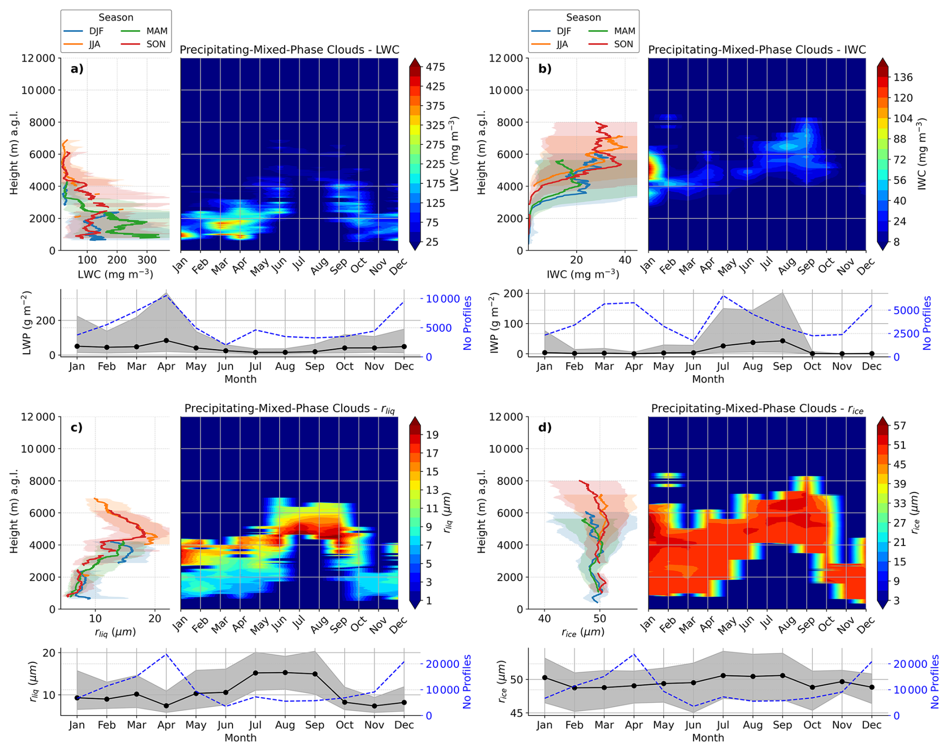
Taken together, precipitating Mixed-Phase clouds exhibit significantly higher LWP compared to IWP, with both exhibiting high variability. These findings are consistent with those observed in Mixed-Phase clouds. The annual median LWP and IWP are 38.3 and 2.9 g m⁻², respectively. Additionally, LWC is predominant at the lower part of the clouds, while the IWC is predominant in the upper part, similarly to non-precipitating mixed-phase clouds. In terms of particle size, r_ice is notably larger than r_liq, with r_ice also presenting the highest variability. The annual median values of r_liq and r_ice are 9.6 and 49.7 µm, respectively. Additionally, r_liq displays more pronounced seasonal variability than r_ice, with notably larger values during summer.

4.3.3 Ice Clouds

Figure 11a shows seasonal and monthly median profiles of IWC and monthly IWP statistics for ice clouds. Seasonal and monthly median profiles of IWC are presented in the top-left and top-right panels, respectively, with monthly IWP statistics in the bottom panel. As shown in the top-left panel, IWC first increases near the cloud base and then decreases with height. This behavior is consistent with previous observations in other sites (e.g., Heymsfield et al., 2002; Sapucci et al., 2007), which showed that in ice-only clouds, ice crystals are typically generated near the cloud top and later they grow by vapor deposition as they fall, leading to an initial increase in IWC with decreasing altitude. However, below this growth region, sedimentation dominates and IWC begins to decrease toward the cloud base as particles fall out or sublimate. Regarding seasonal comparisons, winter and spring exhibit similar vertical profiles, with maxima around 24 mg m⁻³ at 6 km, primarily driven by high values in December (winter) and in March and April (spring), as indicated in the top-right panel. Summer and fall also show comparable profiles, with IWC maxima of 28 and 22 mg m⁻³ at 7 km, associated with maxima observed in June and August (summer) and in October (fall). The bottom panel reveals high interquartile variability in IWP, with minimum monthly median ranging from 2 g m⁻² in July to 12–13 g m⁻² in April and September. However, the monthly medians are much less variable, with values typically closer to the annual median of 8.5 g m⁻².

For precipitating ice clouds, seasonal IWC profiles and IWP distributions are shown in Fig. 11b. The vertical structure of IWC on top-left panel typically shows an increase at mid-levels followed by a decrease at higher altitudes. This pattern has been observed in deep convective clouds, where strong updrafts transport ice particles upward, promoting growth by vapor deposition and aggregation (Fridlind et al., 2015; Jensen et al., 2018). At upper levels, reduced moisture availability and enhanced sedimentation lead to a decrease in IWC (Fridlind et al., 2015). During summer and fall, nearly identical IWC profiles, both with maximum of 150 mg m⁻³ at 7 km are found. These maxima can be associated with high values in June and September, as indicated in the top-right panel. Spring and winter also display similar profiles, with peaks of 70 and 130 mg m⁻³, respectively, around 4.6 km. The winter maximum is mainly driven by December observations, while the spring maximum is observed to May. The bottom panel shows a maximum IWP of 400 g m⁻² in February (winter), and the highest interquartil variability in September (fall). This maximum is larger than the annual median of 122 g m⁻², showing substantial variability compared to only-ice clouds.

The vertical structures of r_ice for ice clouds are examined in Fig. 11c. According to the top-left panel, r_ice generally increases slightly near the cloud base and then decreases with height. This agrees with observations in other places showing depositional growth at lower levels and smaller ice crystals near the cloud top (Heymsfield et al., 2002). Summer and fall exhibit similar vertical profiles, with slightly larger values in summer, while winter and spring also show comparable profiles, with slightly larger radius in spring, above 8 km. In all seasons, r_ice first appears with approximately 47 µm before decreasing with height, although it occurs at higher levels during summer and fall. This behavior is consistent over all months as can be seen by the monthly profiles in the top-right panel. The bottom panel indicates moderated variability of monthly r_ice, with annual median of 38.6 µm and maximum of 43 µm in July.

For precipitating ice clouds, similar seasonal patterns are observed (Fig. 11d). The top-left panel show that r_ice generally increases with height up to a certain altitude before it starts to decrease. This behavior is consistent with microphysical evolution of glaciated clouds, where ice particles grow through vapor deposition and aggregation in the lower and mid-levels of the cloud. At higher altitudes, reduced water vapor availability, enhanced sublimation, and the sedimentation of larger particles lead to a reduction in particle size (Heymsfield et al., 2002). In winter and spring, r_ice remains almost constant, showing only a light increase, up to 5 km, reaching a maximum of approximately 53.0 µm, followed by a rapid decrease. These peaks are primarily associated with enhanced values observed in February and December. Summer and fall also exhibit a similar pattern, but the maximum occurs now at higher altitudes (6 km), with maximum values of 56.0 µm, mainly due to observations in June and September. The bottom panel shows larger ice particles in comparison with only-ice clouds. The monthly median values of r_ice present slight variations around the annual median of 50.5 µm, with biggest particles in September.

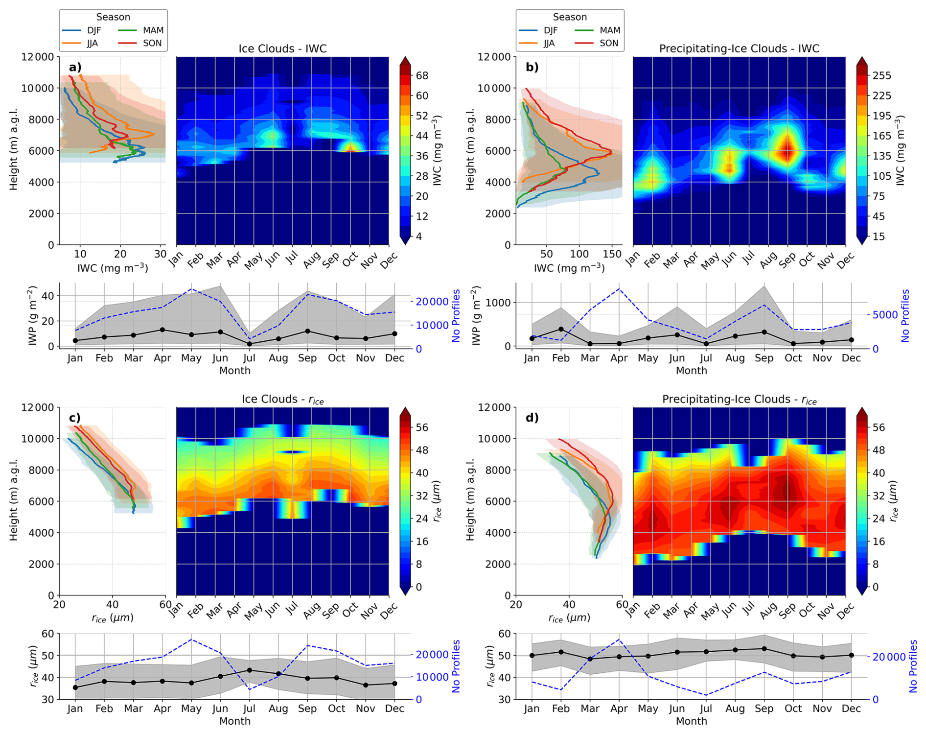
Figure 11 Seasonal and monthly profiles of microphysical properties for ice clouds and precipitating ice clouds. For ice clouds, (a) presents median vertical profiles of IWC by season (a, c), by month (b, d), and monthly median IWP (c, d). (c) shows vertical profiles of ice effective radius (r_ice) by season (a, c), by month (b, d), and monthly r_ice statistics in the bottom panel. (b) and (d) present the same as (a) and (c), respectively, but for precipitating ice clouds. Shaded areas denote the interquartile range, and the blue lines in bottom panels indicate the number of profiles used in each month.

Overall, precipitating ice clouds exhibit significantly larger IWP and effective radius r_ice compared to non-precipitating ice clouds. The annual median IWP for precipitating ice clouds is approximately 121 g m⁻², while for non-precipitating ice clouds it is 8.5 g m⁻². Similarly, the annual median r_ice is about 50.5 µm for precipitating cases, compared to 38.6 µm for non-precipitating ones. In general, IWP shows much greater variability than r_ice, whereas r_ice presents a more consistent and well-defined vertical structure. Additionally, ice clouds exhibit IWC and r_ice values at higher altitudes, consistent with their observed cloud base and top heights (see Fig. 7).

4.4 Structural and microphysical comparison between cloud types

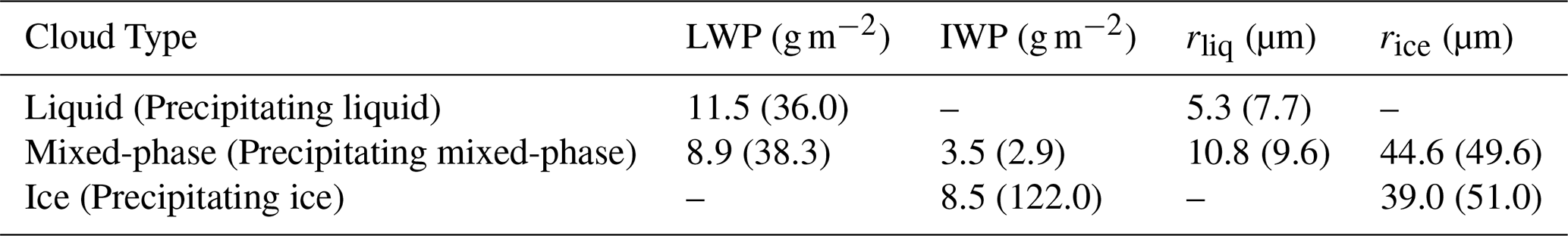
In summary, considering only non-precipitating clouds, liquid clouds are the thinnest (∼ 150 m), exhibit the lowest CBH, the smallest r_liq (5.3 µm), and a LWP of approximately 11.5 g m⁻² (see Tables 2 and 3). Mixed-phase clouds are thicker (∼ 700 m), with higher CBH and larger r_liq (10.8 µm), while their LWP is comparable to that of liquid clouds (8.9 g m⁻²), though slightly lower. These clouds exhibit lower IWP values (3.5 g m⁻²) and an average r_ice of 44.6 µm. Next, ice clouds at our site are thicker than mixed-phase clouds, with higher CBH, higher IWP (8.5 g m⁻²), and slightly smaller r_ice (39.0 µm).

In precipitating cases, cloud thickness and LWP increase markedly, while CBH decreases (see Tables 2 and 3). For precipitating liquid clouds, the average thickness doubles compared to non-precipitating cases, reaching approximately 360 m. Both LWP and droplet size (r_liq) also increase, with values of 36.0 g m⁻² and 7.7 µm, respectively. Precipitating mixed-phase clouds are slightly thicker than non-precipitating ones (∼ 980 m), with most of the increased depth associated with liquid water. LWP rises to 38.3 g m⁻², while IWP slightly decreases to 2.9 g m⁻². In these clouds, r_ice increases to 49.6 µm, while r_liq remains comparable to the non-precipitating case, though slightly smaller. Indeed, these clouds have LWP values similar to those in precipitating liquid clouds, but with marginally larger r_liq. Precipitating ice clouds are the deepest among all cloud types (3.7 km), exhibiting the highest IWP (122.0 g m⁻²) and largest ice r_ice (51.0 µm). These clouds contain substantially more IWP than precipitating mixed-phase clouds, and similar r_ice.

Table 3 Annual median of microphysical properties per cloud type.

It is worth noting that the microphysical profiles discussed in previous section (i.e., LWC, IWC, r_liq, and r_ice) exhibited similar behavior between summer and fall, as well as between winter and spring. These seasonal similarities are particularly more pronounced for ice properties than liquid ones properties, suggesting comparable atmospheric conditions during cloud formation in these respective periods. This interpretation is supported by previous studies, which reported similar vertical profiles of temperature and relative humidity between winter and spring, and between summer and fall (Bedoya-Velásquez et al., 2019).

5 Summary and outlook

This study exploited five years of ground-based Cloudnet measurements (i.e cloud Doppler radar at 94 GHz, microwave radiometer, and ceilometer) to achieve a statistical analysis of cloud properties at the AGORA-ACTRIS CCRES station. The aim is to characterize different types of clouds using Cloudnet post-processed data, focusing on single-layer clouds, in the under-sampled Western Mediterranean region. This study showed that the characterization of the different cloud types strongly depends on the cloud classification algorithm used, which can introduce strong unrealistic correlations between cloud types if not properly defined. To overcome this issue, a novel cloud classification algorithm named cluster-based algorithm (CBA) is presented here. This algorithms considers the volumetric aspect of clouds and generate much better correlation between ice and mixed-phase clouds.

Overall cloud occurrence at the AGORA station shows low cloudy occurrence, with clear-sky conditions prevailing year-round, except in spring. Precipitating liquid clouds are the least frequent, with a total occurrence of 1.2 %, followed by liquid clouds (1.4 %). Precipitating mixed-phase and mixed-phase clouds occur in 3.2 % and 3.4 % of the cases, respectively. Precipitating ice clouds are more common (3.6 %), while ice clouds are the most frequent, accounting for 5.0 % of all observations.

Liquid clouds usually have low CBH (∼ 1.4 km), except in summer when the base height is nearly double (2.09 km). Their monthly r_liq are nearly constant at 5.3 µm. In contrast, precipitating liquid clouds have lower CBH (830 m), generally below 1 km (except in summer), and are about twice as thick as non-precipitating ones (360 m). They also have higher LWC and larger droplets, with maximum in November (9.6 µm), respectively.

Mixed-phase clouds have shown strong seasonal variation in CBH, with minimum in winter (4.77 km) and the maximum in fall (6.5 km). Their LWC is mostly below 4 km, while IWC dominates above that level. Both r_liq and r_ice have maximum around 4 km before decreasing with height. They have larger thickness and higher CBH than liquid clouds, with larger droplets and similar LWP. Precipitating mixed-phase clouds have much lower CBH (∼ 1.53 km) and are about 300 m thicker. Their droplet and ice particle sizes are also larger.

Ice clouds have the highest CBHs, roughly around 7.7 km. Their r_ice decreases with altitude above the level where IWC reaches its maximum. They are thicker and highest than mixed-phase clouds, containing more ice but slightly smaller r_ice. Precipitating ice clouds have much lower CBH (at 2 km), with minimum in winter/spring, and maximum in summer. They also show high variability in thickness and have much higher IWC than only ice clouds. In general, ice properties (i.e. IWC and r_ice) for both ice and mixed-phase clouds exhibited similar vertical profiles between summer/fall, and between winter/spring.

The detailed characterization of cloud types observed at the ACTRIS-CCRES AGORA station offers valuable reference data for model and satellite retrievals validation. Large Eddy Simulation (LES) models and satellite-based observations can benefit from these results, especially for the Iberian Peninsula, where there is no other cloud remote sensing database available.

In the light of the findings presented throughout this paper, future work should focus on identifying and flagging strong attenuation effects, particularly in precipitating clouds. It can contribute significantly to the observed variability in cloud microphysical properties, and cloud thickness. In mixed-phase clouds, coexistence of ice and liquid droplets can generate inaccurate retrievals of liquid and ice properties. This issue can be mitigated by analyzing Doppler spectra, separating the spectral regions associated with ice and liquid to perform more accurate, phase-specific retrievals. Moreover, a deeper physical understanding of the relationships between cloud types is crucial for improving the accuracy and robustness of cloud classification algorithms.

Appendix A: Profile-based algorithm

The Profile-based algorithm (PBA) classifies clouds by individual profiles (Pîrloagă et al., 2022; Nomokonova et al., 2019; Kneifel et al., 2022). The PBA uses the target classification (TCP) from Cloudnet to classify sequences of pixels with height. For each time step, vertical sequences of pixels in TCP are classified as follow:

1. Cloud layer criteria: More than 3 consecutive hydrometeor pixels (38–153 m) (Nomokonova et al., 2019) are considered a cloud layer.

   • (a)

     Liquid criteria: Sequence of only “Droplets” and “Drizzle & Droplets” pixels

   • (b)

     Ice criteria: Sequence of only “Ice” pixels

   • (c)

     Mixed-Phase criteria: Sequence of only “Droplets”, “Ice”, “Ice & Droplets”, “Melting ice”, “Melting & droplets”, “Drizzle and droplets” pixels

   • (d)

     Rain criteria: For Liquid or Mixed-Phase clouds, if more than 1 pixel of “Drizzle or rain” is found below the cloud layer, then it is considered as a precipitating layer. Thus, this cloud layer is then classified as Precipitating Liquid cloud or Precipitating Mixed-Phase cloud.

2. Multilayer classification

   • (a)

     Multi-layer criteria: More than 4 pixels (64–255 m) (Pîrloagă et al., 2022) of any combination of “Clear sky”, “Aerosol”, “Insect” and “Aerosol & insect” between cloud layers. Otherwise, it's a single layer cloud.

Appendix B: Pixel dilatation

The dilation method consists of expanding hydrometeor pixels to connect the closest clusters of hydrometeors, which are likely to belong to the same cloud. To illustrate the method, Fig. B1a shows the TCP product from Cloudnet (11 February 2021), while Fig. B1b shows the hydrometeor clusters, represented by different colors. These clusters were dilated by one pixel in all directions, merging neighboring clusters separated by at most two pixels. Then, the pixels were contracted to return to their original coordinates, while merging the coordinates of closest clusters into a single one. For example, this can be seen in the same color attributed to neighboring clusters within the black circle in Fig. B1b.

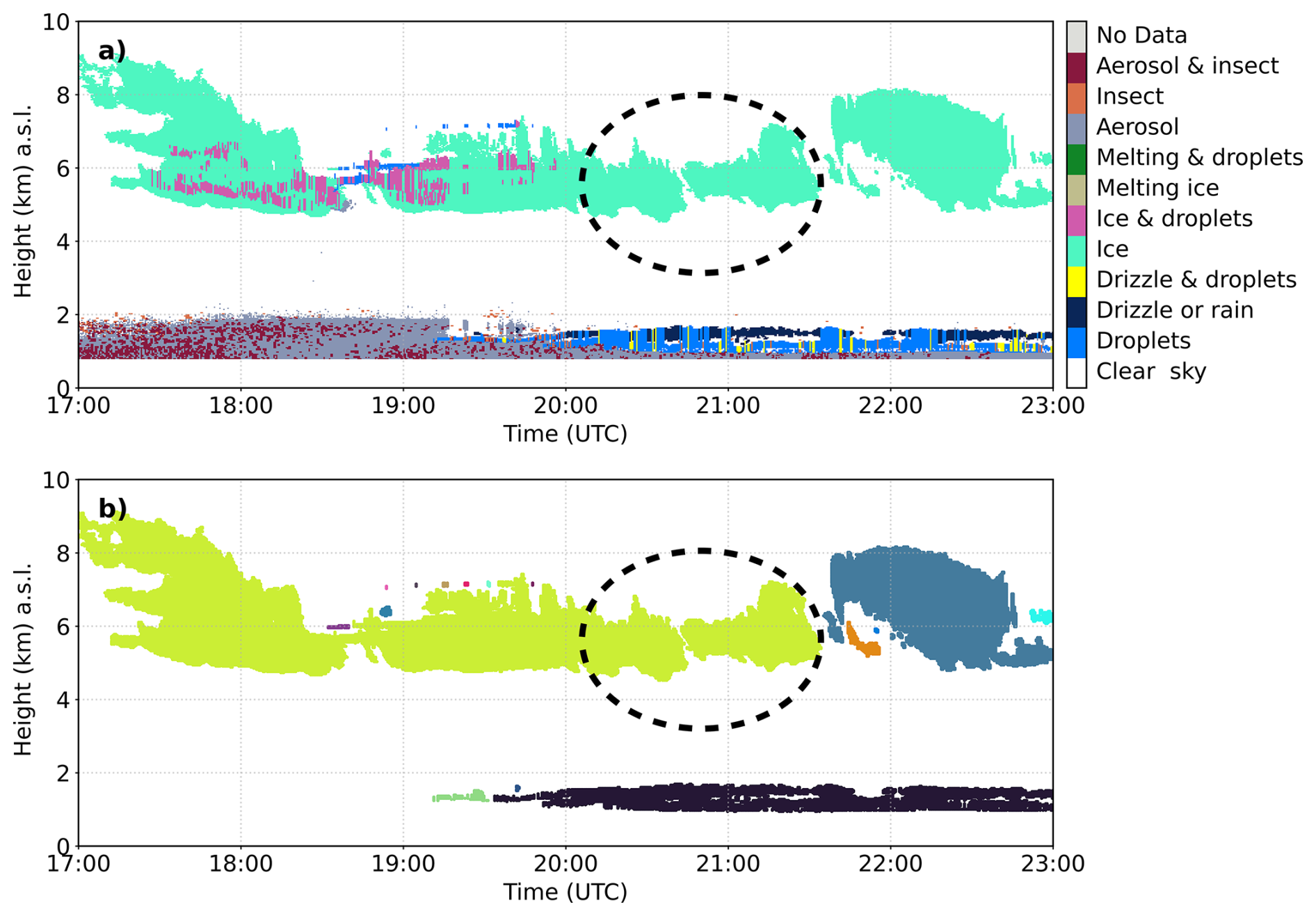
Figure B1 Cluster identification by Cloudnet TCP on 11 February 2021. (a) Target classification, which shows particles typing in time and height. (b) Cloud clusters identified after pixel dilatation and contraction. Each color represents a different cluster, and the dashed black circle indicates the merge of the nearest clusters. Note that differences in resolution between figures may occur due to different plotting schemes, where Fig. B1a is an image plot and Fig. B1b is a scatter plot.

Appendix C: Sensitivity analysis to cloud classification thresholds

A sensitivity analysis is performed to assess the robustness of the cloud statistics against the classification thresholds defined in Sect. 3. Figure C1 shows the annual variability of cloud occurrence and cloud properties (i.e., CBH, cloud thickness, LWP, IWP) obtained using different threshold values. The results obtained using the values adopted in Sect. 3 are indicated by dashed lines and square markers and are used as reference. The shaded areas represent the range spanned by the minimum and maximum thresholds tested, delimited by narrow and thick lines, respectively.

The cloud pixel threshold is varied between 60 and 140 pixels in steps of 20 pixels, with 100 being the value used in Sect. 3 (i.e., Cloud criteria). No significant changes are observed in cloud occurence, CBH, thickness, LWP, or IWP (Fig. C1a–e). The annual patterns remain unchanged, indicating that the results are not sensitive to reasonable variations in cluster size.

The liquid fraction threshold was varied between 60 % and 90 %, with 70 % used as the reference value in Sect. 3 (i.e., Liquid criteria). The monthly frequency for each cloud type is shown in Fig. C1f, where the largest frequency differences are observed for Liquid/Precipitating Liquid (in blue/dark blue) and Mixed/Precipitating Mixed clouds (in yellow/orange), with respective absolute frequency differences of 0.57 % $/$ 0.61 % and 0.57 % $/$ 0.62 %, respectively. This figure shows that as the threshold increases toward 90 %, the frequency of liquid clouds decreases, whereas that of mixed-phase clouds increases. Nevertheless, the seasonal cycle is preserved for all thresholds, and the magnitude of the differences remains within an acceptable range. The CBH, thickness, and IWP are not significantly sensitive to the liquid fraction threshold (Fig. C1g, h, and j). Larger differences are observed for LWP in precipitating liquid clouds during January (dark blue in Fig. C1i), which can be attributed to their very low occurrence and high variability during this month. Therefore, results obtained under limited sampling conditions should be interpreted with caution.

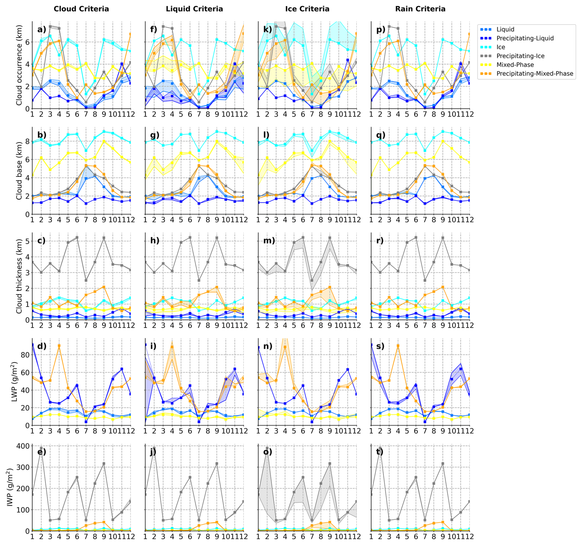
Figure C1 Sensitivity analysis of cloud properties for cloud criteria (a–e), liquid criteria (f–j), ice criteria (k–o), and rain criteria (p–t). For each criteria, cloud occurrence (a, f, k, p), CBH (b, g, l, q), cloud thickness (c, h, m, r), LWP (d, i, n, s) and IWP (e, j, o, t) were analysed for the threshold variations described in the text. Each cloud type is indicated in the legend and Ice clouds are not shown in LWP analysis and liquid clouds are not shown in IWP analysis.

The ice fraction threshold was varied between 80 % and 100 % in steps of 5 %, with a value of 90 % used in Sect. 3 (i.e., Ice criteria). Differences in frequency are observed between ice and mixed-phase clouds (cyan and yellow, respectively, in Fig. C1k), where increasing the threshold leads to fewer ice clouds and more mixed-phase clouds. However, the seasonal cycle remains consistent across all tested values, and total frequency differences remain below 1.5 %. Changes in the ice fraction threshold do not significantly affect CBH, thickness, and LWP (Fig. C1l–n). Although IWP for precipitating ice clouds (in grey) shows larger differences (Fig. C1o), the 90 % threshold used in this study yields values very close to those obtained with the strictest criterion (100 %), indicating that a 90 % threshold is sufficiently robust for classifying ice clouds.

The rain pixel threshold was varied between 5 and 15 pixels, with a value of 10 pixels used in Sect. 3 (i.e., Rain criteria). No significant differences are found in the cloud occurence, CBH, thickness, LWP, or IWP (Fig. C1p–t). The annual patterns remain unchanged, indicating that the results are insensitive to reasonable variations in the rain pixel criterion.

Overall, the sensitivity analysis demonstrates that the main results and conclusions of this study are robust to reasonable perturbations of the thresholds defined in Sect. 3. The variations in cloud occurrence and properties observed for each criterion indicate that seasonal patterns are preserved, and differences from the values used in this study (see Sect. 3) are not statistically significant. This confirms that the proposed CBA and its conclusions are not sensitive to the particular choice of thresholds within physically meaningful ranges