Experiments with a large number of GNSS-RO observations through the ROMEX collaboration in the Met Office NWP system

Over recent years there has been an increase in the number of global navigation satellite system – radio occultation (GNSS-RO) observations available for use in numerical weather prediction (NWP). The Radio Occultation Modelling Experiment (ROMEX) was set up to assess the impact of increasing numbers of GNSS-RO observations and to provide evidence for a further increase in the number. Unlike previous studies, ROMEX gathered a large set of real observations to test the impact, rather than use simulated observations.

Whilst the final conclusion is that the ROMEX observations have a beneficial impact, the initial tests with the expanded dataset demonstrated a degradation in forecast performance, largely due to forecast biases in geopotential height. This bias is shown to be due to the impact of GNSS-RO observations in the stratosphere. The forward operator for GNSS-RO has a long “tail” meaning that the NWP system is able to adjust the height of observations in the stratosphere by changing the tropospheric state (i.e. raising or lowering the height of the observation). Thus, the NWP system can adjust to a systematic difference between the model and observations in the stratosphere by creating a bias in the tropospheric state. Therefore, it was necessary to adjust the refractivity operator used in the forward model to reduce this bias in the forecast state. After much experimentation it was decided to alter the refractivity coefficients in the operator by 0.05 % and 3.5 % for k₁ and k₂, respectively. When using this adjusted operator it was possible to demonstrate the beneficial effect of assimilating the ROMEX observations.

Additional modifications were also applied to the processing of GNSS-RO observations, including vertical smoothing of the observed profiles, and a bias correction at high altitudes to correct for errors within the NWP model. With this modified operator various experiments were conducted to assess impact of increases to the total number of observations. It was shown that the addition of the extra ROMEX observations provided a substantial improvement in the forecast quality. This is particularly true in the southern-hemisphere extra-tropics where the largest benefits were seen for the additional data. The benefit seen for a given number of additional observations varied substantially with the region being considered and the data against which the verification was being performed. Overall the largest forecast improvements were seen when assimilating 20 000 occultations per day. An alternative dataset was also created with 20 000 occultations per day, but with a different choice of satellites. This alternative dataset gave smaller benefits than the official one, indicating that differences in the properties of the observation data source are important and not simply the number of observations.

1 Introduction

1.1 The use of GNSS-RO observations in NWP

Numerical weather prediction (NWP) has brought great benefit to society over many years. NWP forecasts have been gradually improving in quality over time (Bauer et al., 2015). This is due to improved numerical models, increased numbers of observations and improved methods for assimilating those observations.

Radio occultation (RO) observations from global navigation satellite systems (GNSSs) provide one source of observations to the global observing system. These measurements use the time delay in receiving signals from GNSS satellites at a low-Earth orbiting (LEO) satellite, caused by refraction of these signals in Earth's atmosphere. As the LEO orbits Earth the GNSS satellite will appear to rise above or set below Earth's horizon, depending on the relative motion of the satellites. Thus a sequence of observations of the amount of refraction provides a profile through Earth's atmosphere – each such profile is referred to as an occultation. For more information, see for instance Kursinski et al. (1997) and Anthes (2011).

Over recent years the number of GNSS-RO observations has been steadily increasing. This has been largely driven by the launch of the COSMIC-2 constellation (Schreiner et al., 2020), Sentinel-6A and the purchase of observations from private companies such as Spire (Bowler, 2020a) and PlanetIQ (Mo et al., 2024).

The Coordination Group for Meteorological Satellites (CGMS) provides recommendations on the number of observations that should be made each day with the various observation platforms. Whilst the CGMS is not able to mandate the number of observations to be made, it does provide guidance to national meteorological centres and world meteorological organisation (WMO) members on the number of observations that should be made. The CGMS high-level priority plan provides the following recommendation (Coordination Group for Meteorological Satellites, 2024b):

Advance the atmospheric radio occultation constellation, with the long-term goal of providing 20 000 occultations per day with uniform spatial and local time coverage on a sustained basis.

The CGMS also provides a baseline document which further states the target (Coordination Group for Meteorological Satellites, 2024a):

Minimum 6000 occultations from low inclination orbits (< 30°) distributed geographically and temporally in local time, 1000 occultation from other drifting orbits, and 7600 occultations from sun-synchronous orbits. Electron density profiles up to 500 km.

Since the number of observations has increased in recent years, the current number of occultations available daily (approximately 19 400) is now approaching the target of 20 000 occultations per day in the high-level priority plan.

1.2 ROMEX

The Radio Occultation Modelling Experiment (ROMEX; Anthes et al., 2024) was developed as an approach to provide evidence of the impact of increased numbers of GNSS-RO observations on NWP. Previous experiments have considered the impact of simulated observations. However, it was noted that a large number of GNSS-RO observations were available during 2022, largely from commercial providers. With the acquisition of these observations it would be possible to test the impact of increasing the number of observations available without the limitations caused by the use of simulated observations.

ROMEX brought together a large number of organisations from around the world. This included a variety of data providers from Europe, the USA and China, including commercial companies from within those regions. These organisations made their observations available to the project. Most of the data used in ROMEX was processed to bending angles by either the European Organisation for the Exploitation of Meteorological Satellites (EUMETSAT) or the University Corporation for Atmospheric Research (UCAR), which helped to minimise differences or problems in the data. These data were provided to NWP centres within the ROMEX consortium in order to assess the impact of the data on NWP. It was requested that all NWP centres run at least the control experiment (consisting of data from the Metop, COSMIC-2, KOMPSAT-5, PAZ, TerraSAR-X, TanDEM-X and Sentinel-6A satellites) and an experiment with the entire dataset. Additional experiments were suggested, but these were considered optional.

1.3 Previous experiments

The expected impact of increasing the number of GNSS-RO observations on NWP was studied by Harnisch et al. (2013) using an ensemble of data assimilations (EDA). In that study synthetic observations were created, and the impact of the observations were estimated by examining the change in the spread of the ensemble. They simulated 128 000 occultations per day and the effect of using certain fractions of these observations was considered. They found that 16 000 occultations per day gave approximately half the reduction in the ensemble spread of using the full set of observations. Therefore they recommended that 16 000–20 000 globally distributed occultations per day be considered as a minimum requirement for the global observing system.

Prive et al. (2022) conducted an observation system simulation study (OSSE) to assess the impact of increasing the number of GNSS-RO observations. An OSSE uses synthetic observations, like an EDA study. However, the simulated observations are derived using a “nature run” from a model which is independent of the model used to produce the forecasts. Thus the effects of differences between the models will affect the use of the observations. For this reason, we might expect that the results from an OSSE would be more reliable than those from an EDA. They simulated up to 100 000 occultations per day and found that there was no saturation in the benefit to the forecast from assimilating additional data. However, they noted that the rate of improvement diminished after 50 000 occultations per day was reached. They speculated that saturation of benefit might be reached at around 150 000 occultations per day in their system. Their experiment found forecast degradation in certain regions related to the addition of GNSS-RO observations – this was believed to be due to sub-optimal specification of the observation uncertainties for the GNSS-RO data.

2 Experiments with full dataset

All the experiments documented in this report were run using the low-resolution version of the Met Office's global NWP trial workflow. The horizontal resolution of the NWP forecast is described as N320, meaning that it has 640 by 480 grid points, corresponding to a resolution of around 40 km in the mid-latitudes. The model also uses 70 levels in the vertical, stretching from 20 m above the surface to 80 km altitude. The forecasts are for the atmosphere only, and take a prescribed sea-surface temperature from the OSTIA data assimilation system (Fiedler et al., 2019). The atmospheric data assimilation system is a hybrid 4D-Var system (Rawlins et al., 2007; Clayton et al., 2013), meaning that a portion of the background-error covariances are derived from the operational ensemble. The system is run in “uncoupled” mode, meaning that an ensemble forecast is not run as part of the experiments, but the ensemble information is taken from the archive of the operational system. The data assimilation system runs on a 6 h cycle, ingesting observations from a wide variety of sources, including GNSS-RO, microwave and infrared radiances, atmospheric motion vectors, conventional observations and many more. The Met Office's forward operator for GNSS-RO bending angles (Burrows et al., 2014; Burrows, 2014) is a one-dimensional operator. As discussed later, the formulation of Smith and Weintraub (1953) is used in the calculation of the atmospheric refractivity. The observation uncertainties are assigned according to Bowler (2020b), which also gives a brief description of the quality control procedures used for GNSS-RO. For satellites not available at that time an appropriate observation uncertainty estimate is used (Metop-C uncertainties are copied from Metop-A, FY-3E from FY-3C and so on). All other GNSS-RO uncertainties are taken from the COSMIC-1 estimates, although commercial GNSS-RO observations are assumed to have a 6 µrad minimum uncertainty, rather than 3 µrad as is used for most satellites.

For the purposes of running the ROMEX experiments, none of the operationally-available GNSS-RO observations were assimilated. Instead all the GNSS-RO observations are taken from the ROMEX dataset, either for the control set of observations or for the experiment with additional observations. The initial experiment was to compare the control experiment with the experiment using all the ROMEX observations.

Table 1 Summary of all the experiments reported in here. Shown is the averaged percentage change in the RMSE compared to the control. The average is taken over all variables and lead times in the Met Office scorecard. Verification is performed against radiosonde observations (left column) and ECMWF analyses (right column). A negative number indicates that the RMSE is reduced in the experiment.

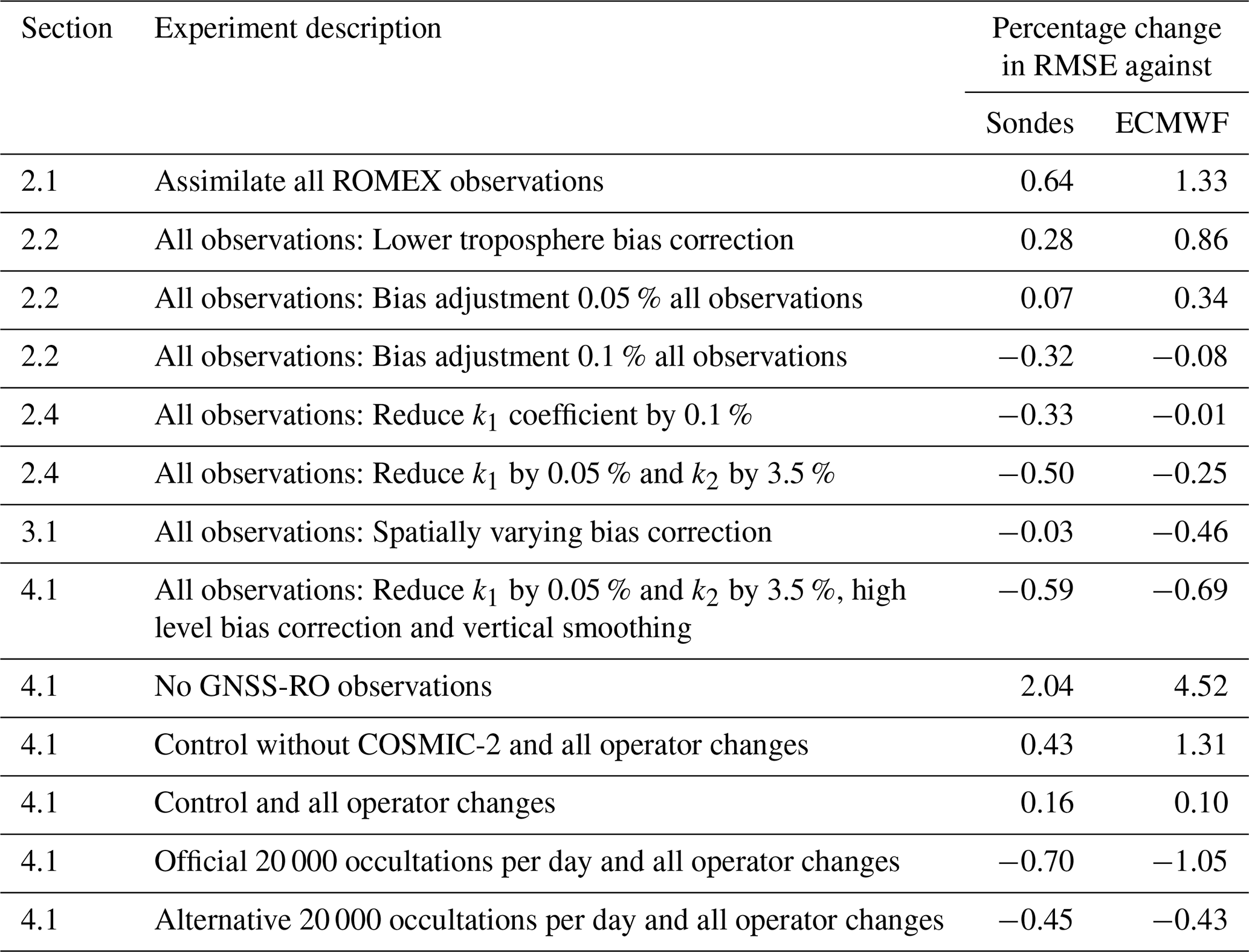
Many experiments have been run assimilating ROMEX data, a selection of which are reported here. Table 1 contains a summary of all the experiments reported here, including which section they are discussed and the average percentage change in the root-mean-square error (RMSE) for the experiment relative to the control. The average is taken over all variables and lead times in the Met Office scorecard (for instance see Fig. 1).

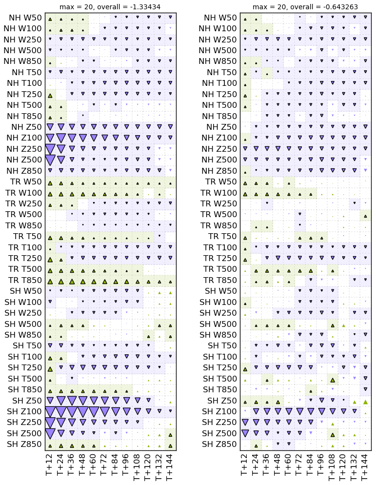
Figure 1 Scorecard showing the change in root-mean-square forecast error for the experiment with all ROMEX observations, compared to the control. The experiments are verified against ECMWF operational analyses (left) and radiosonde observations (right). The area of the triangles is proportional to the fractional change in RMSE. Green (purple-blue) triangles indicate better (worse) performance for the experiment. The y-axis denotes the forecast variable being considered. NH, TR and SH denote the northern hemisphere > 20°, tropics and southern hemisphere < −20°, respectively. The letter following the underscore indicates the weather parameter, with W, T and Z signifying vector wind field, temperature and geopotential height, respectively. The numbers after this indicate the height of the observation in hPa. The x-axis shows the forecast lead time in hours.

2.1 Initial results

A summary of the changes in the RMSE scores for various variables and forecast lead times for the initial experiments assimilating all ROMEX observations, compared to the control, are shown in Fig. 1. Whilst there is an improvement in the forecast for some quantities, such as tropical winds and temperatures at certain heights, there is a large degradation in the extra-tropical forecasts of geopotential height. This is most apparent when considering verification against European Centre for Medium-Range Weather Forecasting (ECMWF) analyses at short lead times. The cause of this degradation is due to a large shift in the bias of the geopotential height forecasts. Figure 2 shows the forecast bias of the control, the experiment assimilating all ROMEX observations, as well as two further experiments which are discussed in the next section. The bias of the short-range forecast becomes strongly negative when the additional observations are assimilated. At longer lead times the forecast drifts towards a positive bias, but this does not appear to lead to improved results in terms of the RMSE (as seen in Fig. 1). Whilst it is hard to be certain about the true value of the average geopotential height of a given pressure level, the shift in the bias is large enough to be confident that it is detrimental change.

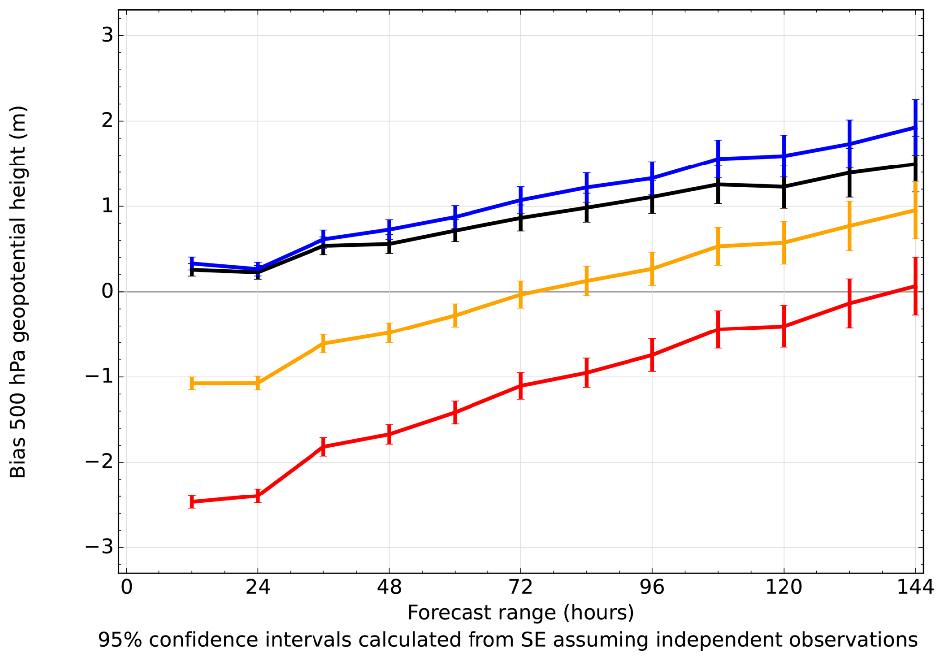
Figure 2 Bias for 500 hPa geopotential height forecasts in the northern extra-tropics, measured against ECMWF analyses. The control experiment (black) is compared to the experiment with all ROMEX observations (red), the experiment with a bias correction of 0.05 % (orange) and the experiment with a bias correction of 0.1 % (blue).

2.2 Investigating the bias by adjusting observations

Since the largest detrimental impacts were seen in geopotential heights which are related to the integral of atmospheric temperature from the surface, it was thought that the sources of the bias would be related to observations in the lower troposphere. Therefore, an experiment was run which adjusted the GNSS-RO observations in this region. The following experiments are not an attempt to indicate that there is any bias in the observations, just test the sensitivity of the results to perturbations in certain regions. Anthes et al. (2025) have investigated the properties of the ROMEX observations and found that the differences between the observation datasets are small. Figure 3 shows the mean difference between the observations and the model background of the observations after quality control, normalised by their average, that is

$$\begin{array}{}\text{(1)}& \mathit{\mu }={\displaystyle \frac{\mathrm{2}}{N}}\sum _{i=\mathrm{1}}^N{\displaystyle \frac{O_i-B_i}{O_i+B_i}}\end{array}$$

where O_i and B_i are the observation and model background values for observation i, respectively, and N is the number of occultations. Each profile of observations is interpolated to a 200 m grid, thus the number of observations is approximately constant in height.

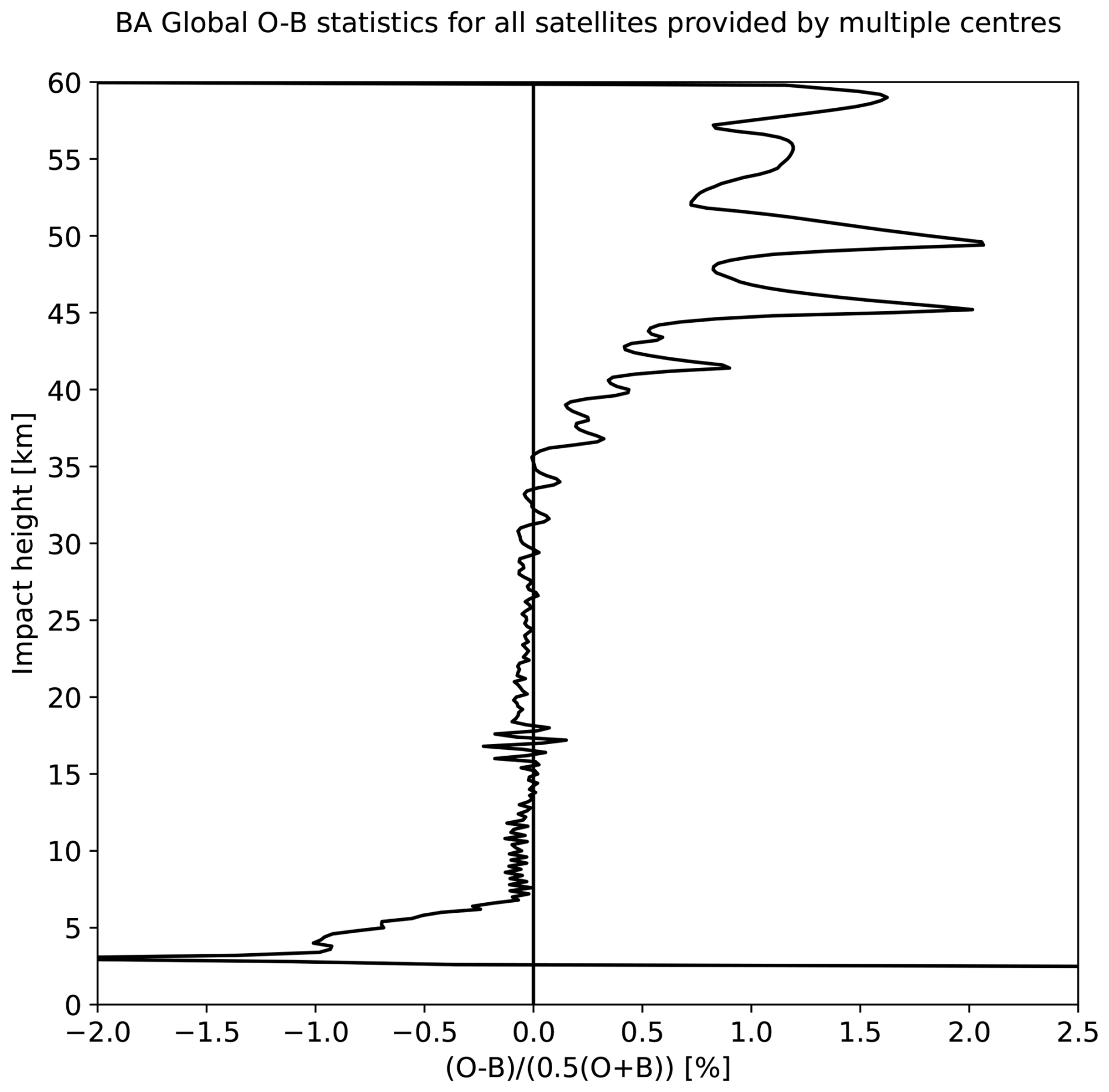
Figure 3 Mean difference between the observations and the model background of the observations, normalised by their average. The data are averaged over all the ROMEX observations.

In the lower troposphere the mean values in Fig. 3 are substantially below zero, indicating that the observations are consistently smaller than the model background. This is a region where data processing choices can affect the bias. For instance, the length of the data record into Earth's shadow can affect lower-tropospheric biases (Sokolovskiy et al., 2010). Between 15 and 20 km there is a small-scale oscillation in the statistics. This is due to the interpolation of the atmospheric quantities from model levels to the impact heights of the observations. These oscillations were reduced by the use of pseudo-levels (Burrows et al., 2014), but were not fully eliminated. If we modify the observed bending angles between 0 and 7 km impact height to be larger, then the bias in O−B in this region will be reduced. An experiment was run where the observed bending angles were adjusted by a factor, linearly increasing from 1 (no adjustment) at 7 km impact height, to 1.025 at 0 km impact height (noting that this is below Earth's surface). This increase is designed to approximately fit the O−B bias seen in Fig. 3. The results of this experiment are shown in Fig. 4. Whilst the overall results have improved, there are still substantial degradations in many forecast quantities relative to the control. In particular, the geopotential height forecasts have improved, but are still substantially degraded compared to the control, especially when verified against ECMWF analyses.

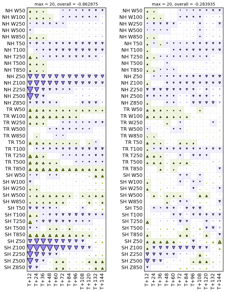
Figure 4 Scorecard showing the change in root-mean-square forecast error for the experiment with all ROMEX observations but with a bias adjustment to observations in the lower troposphere, compared to the control. Figure format as in Fig. 1.

Whilst the geopotential height at 500 hPa represents an integral of the atmospheric state from the surface up to 500 hPa, there is some evidence that we should be considering observations which are located above this level. Eyre (1994) noted that the forward operator for bending angle observations contains sensitivity to the atmospheric state well below the height of the tangent point of the ray. An adjustment to the atmospheric state below the observation will alter the modelled height of the observation, thus adjusting the model forecast of the observation. This has been referred to as a hydrostatic tail for the operator (Bauer et al., 2014). Given this behaviour, one might ask whether the observations at higher altitudes can affect the behaviour of the forecasts of 500 hPa geopotential height. Looking again at Fig. 3, we notice that there is a small negative bias to the O−B statistics between approximately 7 and 30 km impact height. This region is known colloquially as the “golden region” (Anthes et al., 2025), since it is where the observations are most accurate and are given the highest weight in data assimilation systems. Therefore, it is possible that very small biases in this region can play a role in forecast quality.

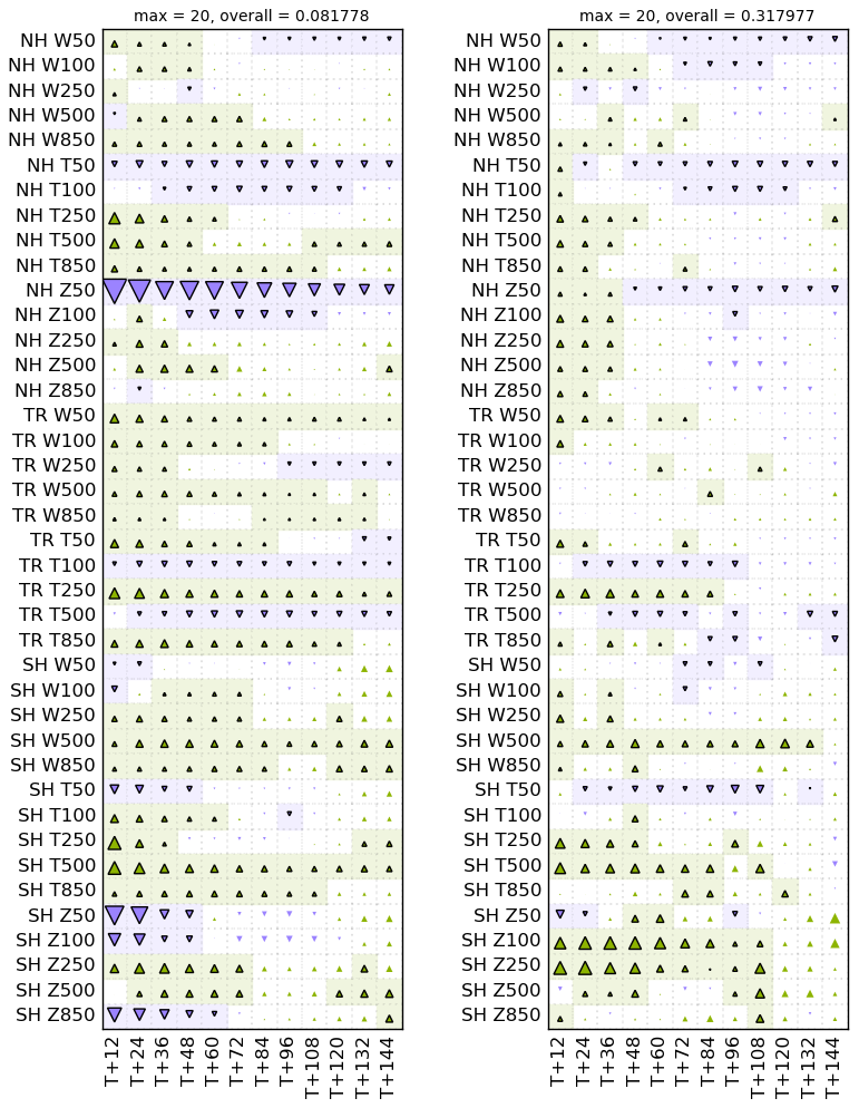
Figure 5 Scorecard showing the change in root-mean-square forecast error for the experiment with all ROMEX observations but with a bias adjustment of 0.1 % to all observations, compared to the control. Figure format as in Fig. 1.

To test this hypothesis, we ran a further experiment where the observed bending angles were increased by 0.05 % throughout the entire profile, since 0.05 % is approximately the difference in the O−B statistics between 7 and 30 km impact height. This experiment performs much better than the initial experiment, especially for tropospheric geopotential heights (not shown). However, the overall performance is still negative for many forecast variables, and therefore we ran a further experiment where all observations are increased by 0.1 %. The results of this experiment are shown in Fig. 5. These results show that by bias correcting the GNSS-RO observations by 0.1 % we achieve a situation where the addition of the ROMEX observations is now a positive change overall, rather than a negative one. Certain results are still negative, such as the 50 hPa geopotential height forecasts measured against ECMWF analyses, and some of the medium-range forecasts when measured against radiosondes. Hence, this bias correction of the observations cannot be regarded as a complete solution.

As previously noted much of the degradation in the forecast quality was due to a change in the bias of geopotential height forecasts in the troposphere. As well as the original results, Fig. 2 shows the forecast bias for 500 hPa geopotential height of the experiments which apply a bias correction to the observations. The experiment which adjusts the observations by 0.05 % approximately halves the negative bias in the short-range forecasts of this quantity. The experiment adjusting by 0.1 % eliminates the negative bias, replacing it with a slight positive bias, similar to the control NWP system. With increasing lead time, the forecast tends towards a positive 500 hPa geopotential height bias. The change of bias in the short-range forecast seems to be the main reason that the adjusted experiments perform better than the initial experiment – they are able to remove the large negative bias in the geopotential height forecasts. Figure 2 shows verification against ECMWF analyses in the northern extra-tropics. Similar results are seen in the southern extra-tropics and for verification against sondes.

2.3 Demonstrating dependence using 1D-Var

To further understand how this bias arises, we use a 1-dimensional variational (1D-Var) assimilation to examine the analysis increments. A 1D-Var assimilation is run as part of the quality control of observations at the Met Office. If the minimisation does not converge within 20 iterations, then the entire profile of observations is rejected (Bowler, 2020b). The 1D-Var process is not identical to treatment of observations within the 4D-Var minimisation used to initialise the forecasts, since no account is made for the drift of the tangent point, and the same 1D background-error covariance matrix is used for all observations. Nonetheless, analysis increments from this system can provide useful insights.

To demonstrate the behaviour of the ROMEX experiments, we take observations from the second cycle of the experimental period – centred around 06:00 UTC on 1 September 2022. The model background state is taken from the operational suite on that day, and all the ROMEX observations between 03:00 and 09:00 UTC are used in the processing. To show how observations at different heights affect the increment produced by the 1D-Var analysis, the observations were perturbed by multiplying them by the factor 1.001 in various height ranges. The observations were only perturbed if their impact height was within 2.5 km of a given value, where the value was either 5, 10, 15 or 20 km. These perturbed analysis increments were then compared against an analysis without any perturbation.

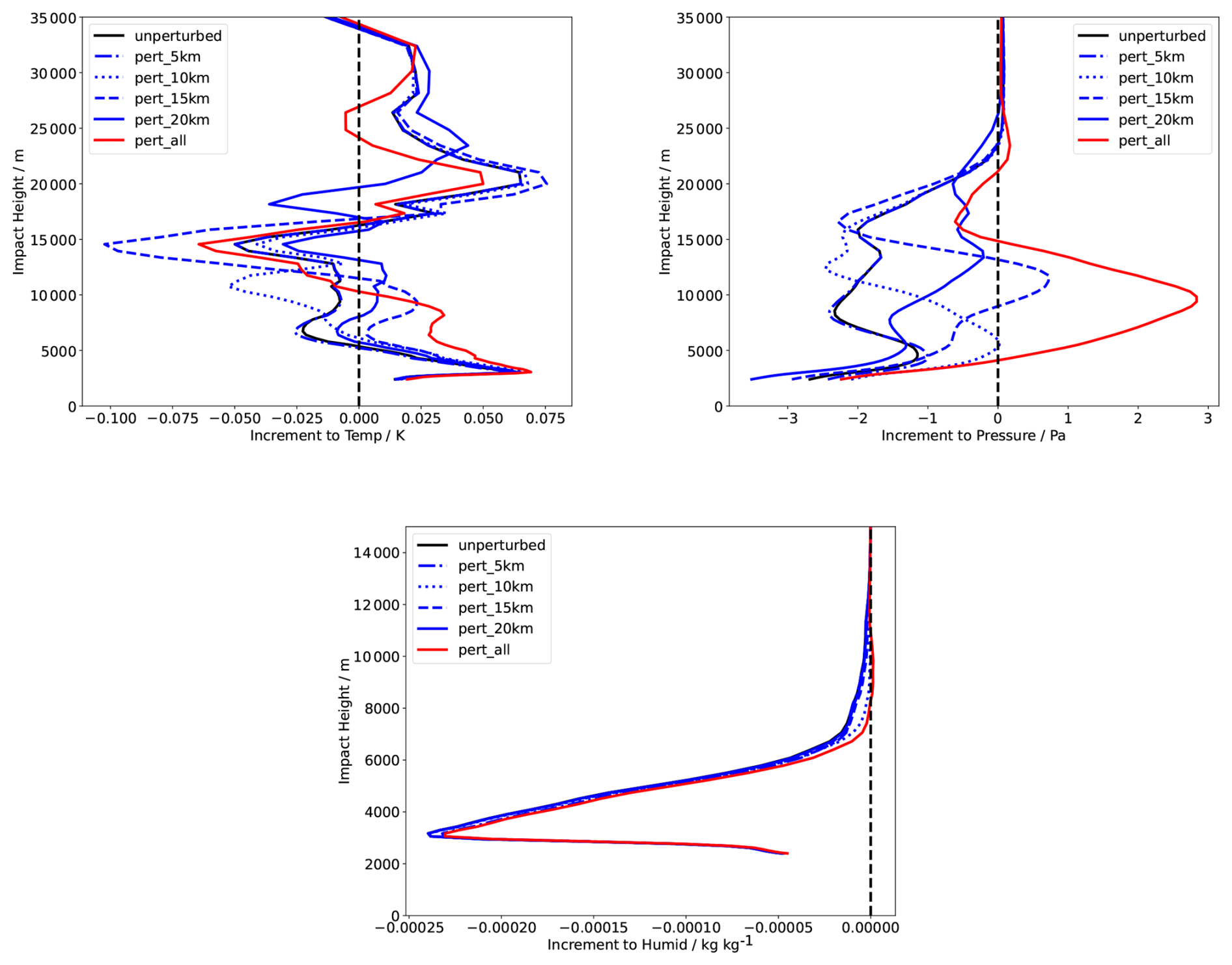
Figure 6 Average analysis increments to temperature (top-left), pressure (top-right) and specific humidity (bottom-left) from the 1D-Var system. Shown are increments from the unperturbed system (blue) and those with perturbations centred on a specific region. pert_all is an experiment where the profile is perturbed at all heights.

Figure 6 shows the analysis increment from the perturbed and unperturbed experiments for pressure, temperature and specific humidity, averaged over all the observations. Since it is a global average, the increment is rather small and potentially changed substantially by the perturbations. Notably, the average increment to pressure is negative below 23 km impact height whereas the temperature increment changes sign at various points in the profile. The average increment to specific humidity is negative, and very similar for both the perturbed and unperturbed simulations.

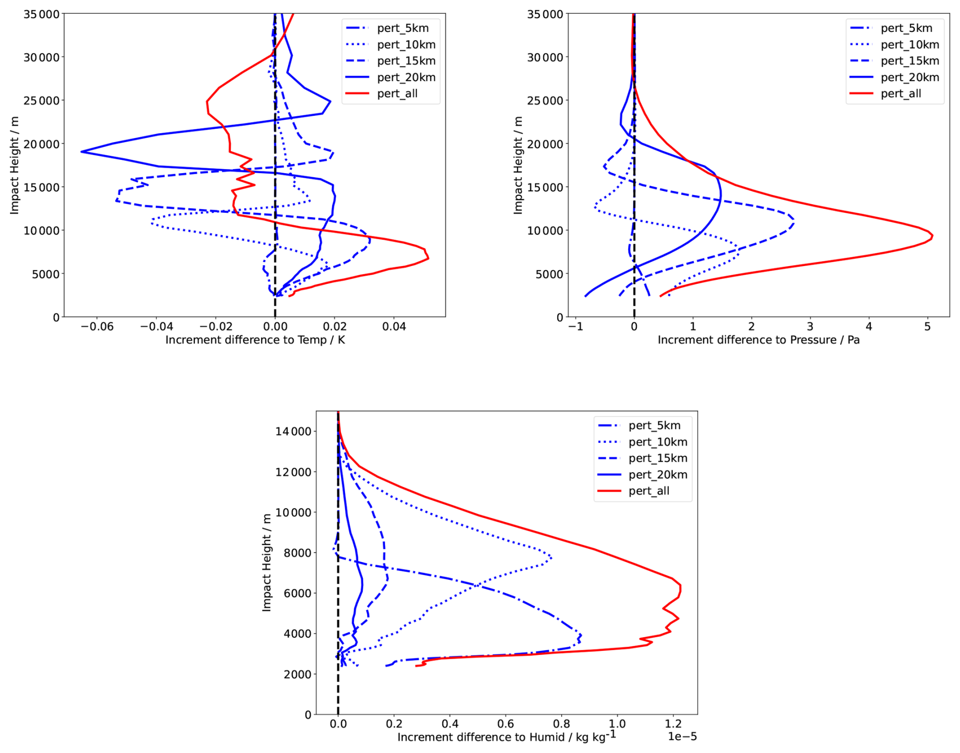
Figure 7 Difference in the analysis increments between the perturbed and unperturbed assimilations. Differences are shown for pressure (top-left), temperature (top-right) and specific humidity (bottom-left).

It is interesting to consider the difference between the analysis increments from the perturbed and unperturbed systems. This is shown in Fig. 7 for temperature, pressure and specific humidity. For temperature, the main change in the increment is a reduction in the temperature at the region where the observations have been perturbed, and an increase at other levels. For pressure, the maximum change is at the bottom of the perturbed region, with an increase in the pressure both within and below the perturbed region. The perturbations to specific humidity serve to increase it, with the largest changes for those perturbations which occur in the troposphere.

The above results indicate that the reduction in the short-range geopotential height forecasts when assimilating the additional GNSS-RO observations is likely due to a systematic reduction in the atmospheric pressure. This is caused by observations in the upper troposphere and above, due to the hydrostatic tail present in the forward operator (Eyre, 1994; Bauer et al., 2014).

2.4 Adjustments to the refractivity operator

Following the experiments adjusting the observations by a constant factor, it was pointed out (Katrin Lonitz, personal communication, 2025) that a very similar effect could be achieved by adjusting the refractivity coefficients in the observation operator. To calculate the refractivity from a model forecast, the Met Office uses the two-term formula of Smith and Weintraub (1953)

$$\begin{array}{}\text{(2)}& N={\displaystyle \frac{k_{\mathrm{1}}p}{T}}+{\displaystyle \frac{k_{\mathrm{2}}e}{T^{\mathrm{2}}}}\end{array}$$

where p is the total atmospheric pressure (including both the dry gases and water vapour, in Pa), T is the temperature in Kelvin, e is the partial pressure of water vapour, also in Pa, k₁ and k₂ are constants derived from laboratory measurements and are k₁=0.776 and $k_{\mathrm{2}}=\mathrm{3.73}\times {\mathrm{10}}^{\mathrm{3}}$. The constants used in this equation are derived from rather old experiments, and more recent formulations of the refractivity may lead to more accurate simulations of the atmosphere (Healy, 2011; Aparicio and Laroche, 2011). Healy (2011) quotes an estimated error of around 0.1 % in the formula for refractivity. Since it is derived from first principles, Aparicio and Laroche (2011) give an estimated error of 0.01 % in their formula. Therefore, assuming changes of 0.1 % in the formula of Smith and Weintraub (1953) is reasonable.

To run an experiment equivalent to the ones above, k₁ was reduced by 0.1 %. The results are very similar to those shown in Fig. 5, and are therefore not included here. Changing the k₁ value gives slightly better forecasts of extratropical temperature and wind, but slightly worse forecasts of extratropical geopotential height. This highlights that a bias correction to the observations can have a very similar effect to an adjustment to the observation operator.

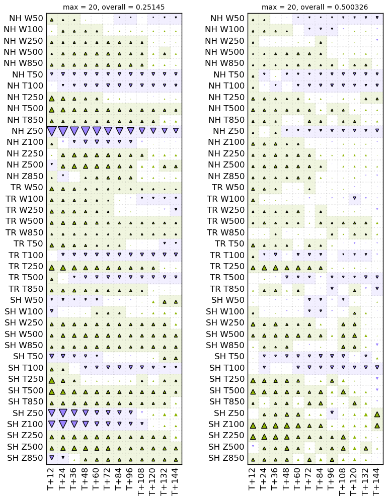
Figure 8 Scorecard showing the change in root-mean-square forecast error for the experiment with all ROMEX observations but with a reduction by 0.05 % of k₁ and a reduction of 3.5 % of k₂ in the refractivity operator, compared to the control. Figure format as in Fig. 1.

Considering Fig. 3 once more, one will note that in addition to the very small bias between 7 and 30 km impact height, there are also large biases in the lower troposphere, as noted previously. Therefore, we consider combining changes to both k₁ and k₂ in the refractivity operator. In order to achieve an approximately unbiased average value of the O−B statistics we reduce k₁ to 0.775612 (a 0.05 % reduction) and k₂ to 3600 (a 3.5 % reduction). Whilst we cannot offer any theoretical justification for either of these changes, they are chosen to approximately match the O−B statistics. With these operator changes, the mean O−B statistics are closer to zero than the statistics shown in Fig. 3. The results of this experiment are shown in Fig. 8. Aside from high altitude geopotential heights against ECMWF analyses, this experiment performs well, with many more positive results than negative ones. The results for geopotential heights in the troposphere are now generally positive, indicating that the former bias issues have been effectively addressed.

2.5 Data assimilation statistics

Another important measurement of the quality of a given change to the data assimilation system is the fit of observations to the model background. Since a 6 h data assimilation window is used, the background forecast lead time is between 3 and 9 h. We measure this using the standard deviation of the difference between the observations and either the model background or the analysis. The ratio of this standard deviation, relative to the same quantity for the control is plotted for each experiment. If this ratio is less than one then it indicates that the experiment has a better fit to the observations than the control. Figure 9 shows this ratio for various observation groups using the background forecast for the experiment which reduced k₁ by 0.05 % and k₂ by 3.5 %. For all three instruments shown, the experiment is closer to the observations for many of the channels. However, for each of the instruments there are some channels where the ratio is greater than one, indicating that the fit to the observations is worse than the control. Cross-track infrared sounder (CrIS) channels with numbers below 25, and Infrared Atmospheric Sounding Interferometer (IASI) channels with numbers below 70 are typically temperature sounding channels which peak in the stratosphere. Similarly, Advanced Microwave Sounding Unit (AMSU-A) channel 8 peaks in the lower stratosphere. Therefore, all those channels for which the addition of GNSS-RO observations has a negative impact are in the stratosphere.

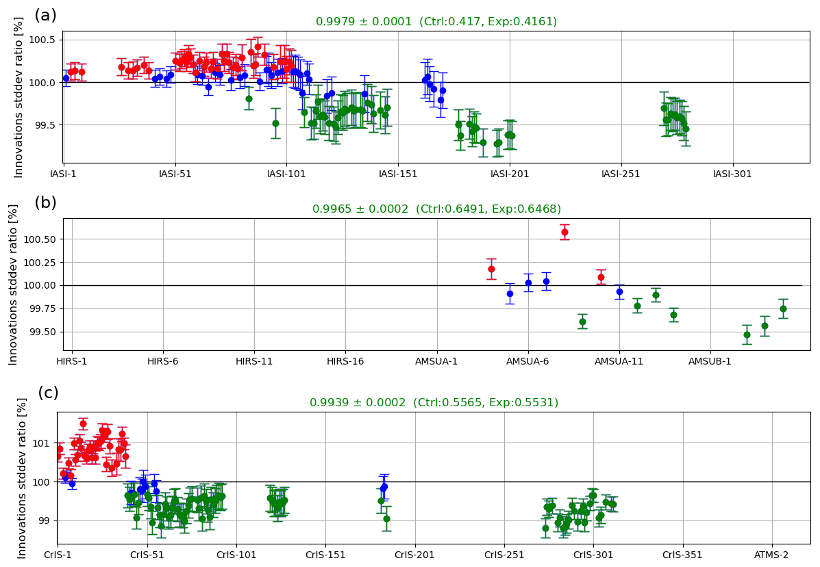
Figure 9 Ratio of the standard deviation of the difference between the observations and model background for the experiment with all ROMEX observations but with a reduction by 0.05 % of k₁ and a reduction of 3.5 % of k₂ in the refractivity operator, compared to the control. Statistics are calculated against (a) IASI observations on Metop-B, (b) ATOVS observations on Metop-C and (c) CrIS observations on NOAA-20. The x-axis shows the Met-Office channel number, which is based on a subset of the full channel set that the Met Office receives for CrIS and IASI.

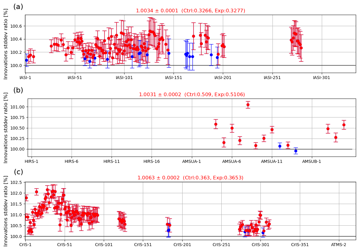
Figure 10 Ratio of the standard deviation of the difference between the observations and model analysis for the experiment with all ROMEX observations but with a reduction by 0.05 % of k₁ and a reduction of 3.5 % of k₂ in the refractivity operator, compared to the control. Statistics are calculated against (a) IASI observations on Metop-B, (b) ATOVS observations on Metop-C and (c) CrIS observations on NOAA-20.

Figure 10 shows the same statistics as Fig. 9, but for the analysis rather than the background. We see that the fit to the observations is degraded for almost all channels when using the analysis. In a perfect system you might expect that adding extra GNSS-RO observations would improve the representation of truth in the analysis leading to improvements of fits to other observations. This is often not the behaviour observed due to differences between observation types including their resolution, coverage, bias etc, which means that one often finds that adding much more of one dataset pulls the analysis away from some others. The overall skill of the analysis might still be improved and give rise to the more widespread (although not universal) improvements in short-range forecast fits.

2.6 Standard deviation of forecast error

The verification results presented above are based on the root-mean-square error of the forecast. It is common instead to consider the standard deviation of the forecast error, as this is unaffected by forecast biases. Typically, the root-mean-square error is calculated using the following formula

$$\begin{array}{}\text{(3)}& \mathrm{RMSE}=\sqrt{{\displaystyle \frac{\mathrm{1}}{N_t}}\sum _{i=\mathrm{1}}^{N_t}{\displaystyle \frac{\mathrm{1}}{N_o}}\sum _{i=\mathrm{1}}^{N_o}{\left(f_{i,t}-o_{i,t}\right)}^{\mathrm{2}}}\end{array}$$

where o_i,t is the verifying reference value at time t and location i, f_i,t is the forecast value, and N_t and N_o are the number of times and locations, respectively. This means that the mean-square error is calculated for each reference time, and then this is averaged over all times. In a similar way, we can calculate the forecast bias via

$$\begin{array}{}\text{(4)}& \mathrm{Bias}={\displaystyle \frac{\mathrm{1}}{N_t}}\sum _{i=\mathrm{1}}^{N_t}{\displaystyle \frac{\mathrm{1}}{N_o}}\sum _{i=\mathrm{1}}^{N_o}\left(f_{i,t}-o_{i,t}\right).\end{array}$$

The calculation of the standard deviation of the forecast error is based on these two quantities

$$\begin{array}{}\text{(5)}& \mathit{\sigma }=\sqrt{{\mathrm{RMSE}}^{\mathrm{2}}-{\mathrm{Bias}}^{\mathrm{2}}}\end{array}$$

where σ is the standard deviation of the forecast error.

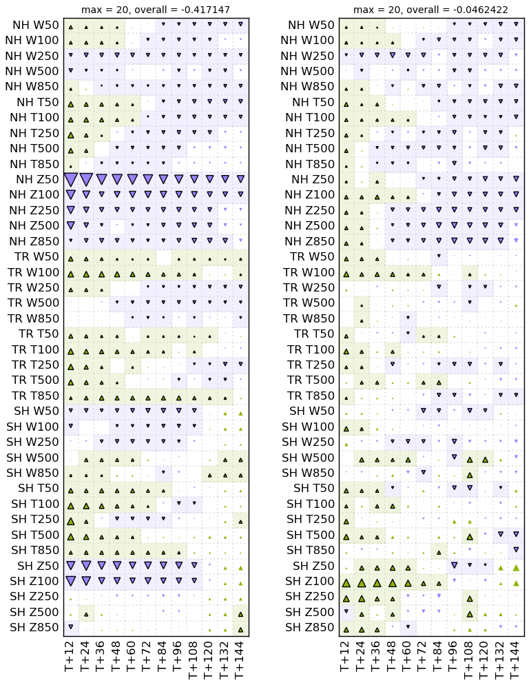
Figure 11 Scorecard showing the change in standard deviation of forecast error for the experiment with all ROMEX observations, compared to the control. Figure format as in Fig. 1.

Experiments at ECMWF, Deutscher Wetterdienst (DWD) and the Joint Center for Satellite Data Assimilation (JCSDA) (Katrin Lonitz, Harald Anlauf, personal communications, 2025; Zhang et al., 2025) demonstrated that the addition of ROMEX observations, without any changes to the operator to account for the bias, resulted in reductions in the standard deviation of the forecast error. Figure 11 shows a scorecard of the standard deviation of the forecast error for the experiment with all ROMEX observations, compared to the control. Like the RMSE scorecard (Fig. 1), there are forecast degradations in many quantities. This is different from the equivalent experiments at ECMWF and DWD. One alternative which was considered is whether the above formulation of the standard deviation of the forecast error affected the results. DWD calculates the standard deviation of forecast error for each verification date (Harald Anlauf, personal communication, 2025) and averages these, rather than calculating the mean-square-error and bias for the entire period. This was attempted, but made very little difference to the results (not shown).

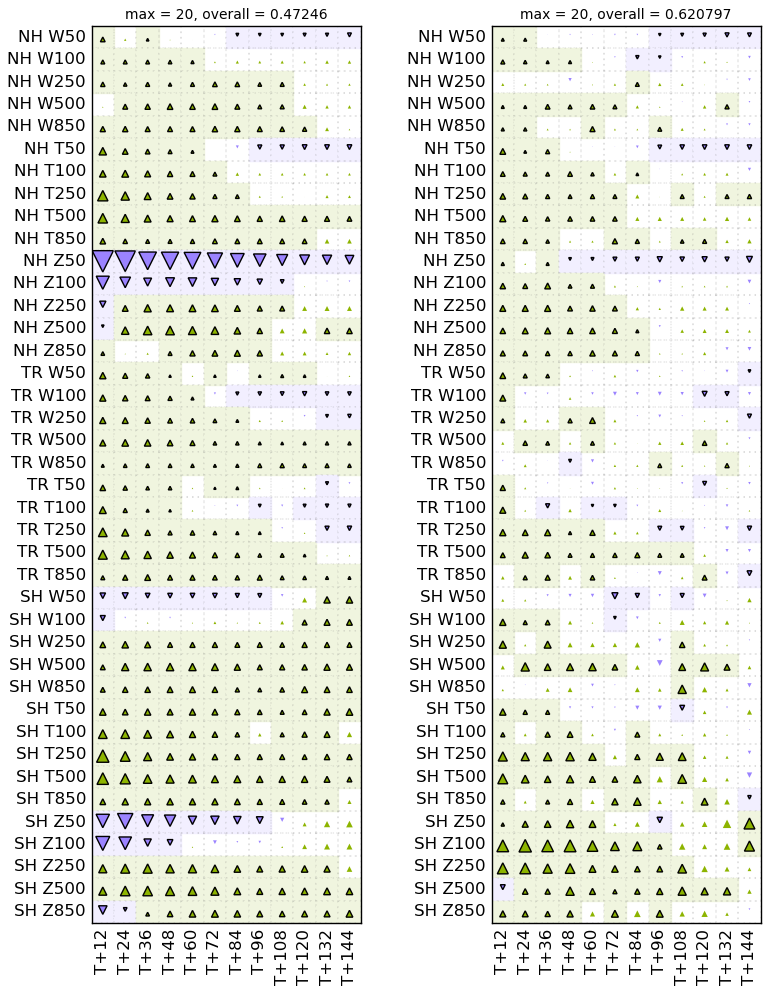
Figure 12 Scorecard showing the change in standard deviation of forecast error for the experiment with all ROMEX observations but with a reduction by 0.05 % of k₁ and a reduction of 3.5 % of k₂ in the refractivity operator, compared to the control. Figure format as in Fig. 1.

When the refractivity operator is adjusted by 0.05 % for k₁ and 3.5 % for k₂, the results for standard deviation are shown in Fig. 12. These results are very similar to those shown in Fig. 8 in that many of the scores are greatly improved, relative to Fig. 11. It is not clear why the bias corrections applied to the operator are having a clear effect on the standard deviation of the forecast error, unlike other centres.

3 Spatially varying bias

Whilst Fig. 3 shows a clear picture that there is an approximately constant bias between the observations and the model background between 7 and 30 km impact height, this does not give the entire picture. Instead, these biases vary both with height and location. Figure 13 shows the variation of the mean O−B statistics with latitude. From this we note that the bias appears to vary quite considerably between the different latitude bands. In the tropics the bias in the troposphere is considerably more negative than at higher latitudes. The rapid variation in the bias in the tropics between 15 and 20 km impact height is due to the interpolation from model levels to impact heights, and therefore is an artefact of the observation operator. In the lower stratosphere there is a negative bias at mid and high latitudes, but a slight positive bias in the tropics. This is suggestive that the adjustments to the coefficients k₁ and k₂ may be too simple to properly account for the bias issues. However, we should note that these statistics make no separation between biases in the observations (which we normally assume to be small) and biases in the model background (which are often known to be large).

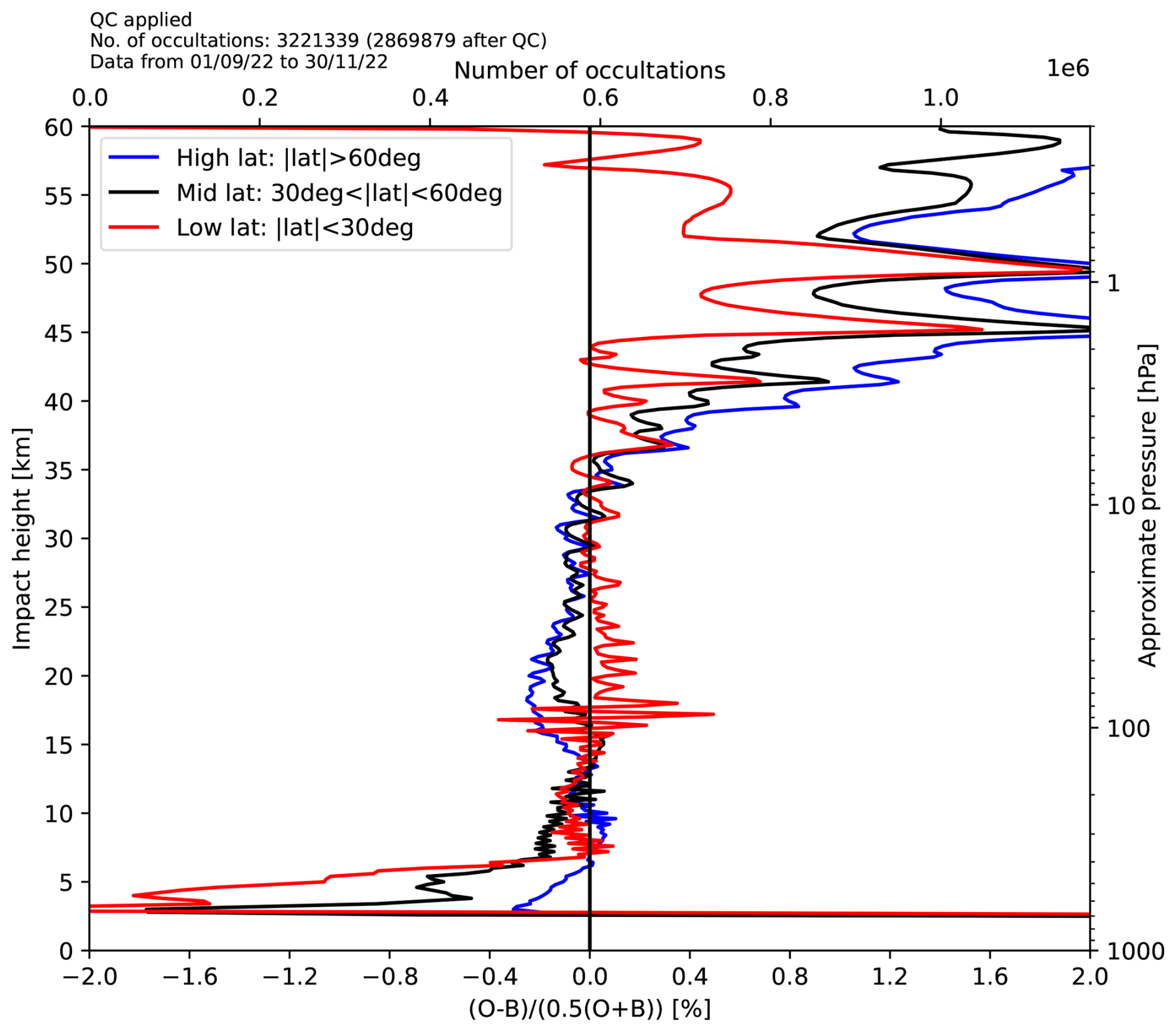
Figure 13 Mean difference between the observations and the model background of the observations, normalised by their average. The data are averaged over all the ROMEX observations, but binned by latitude.

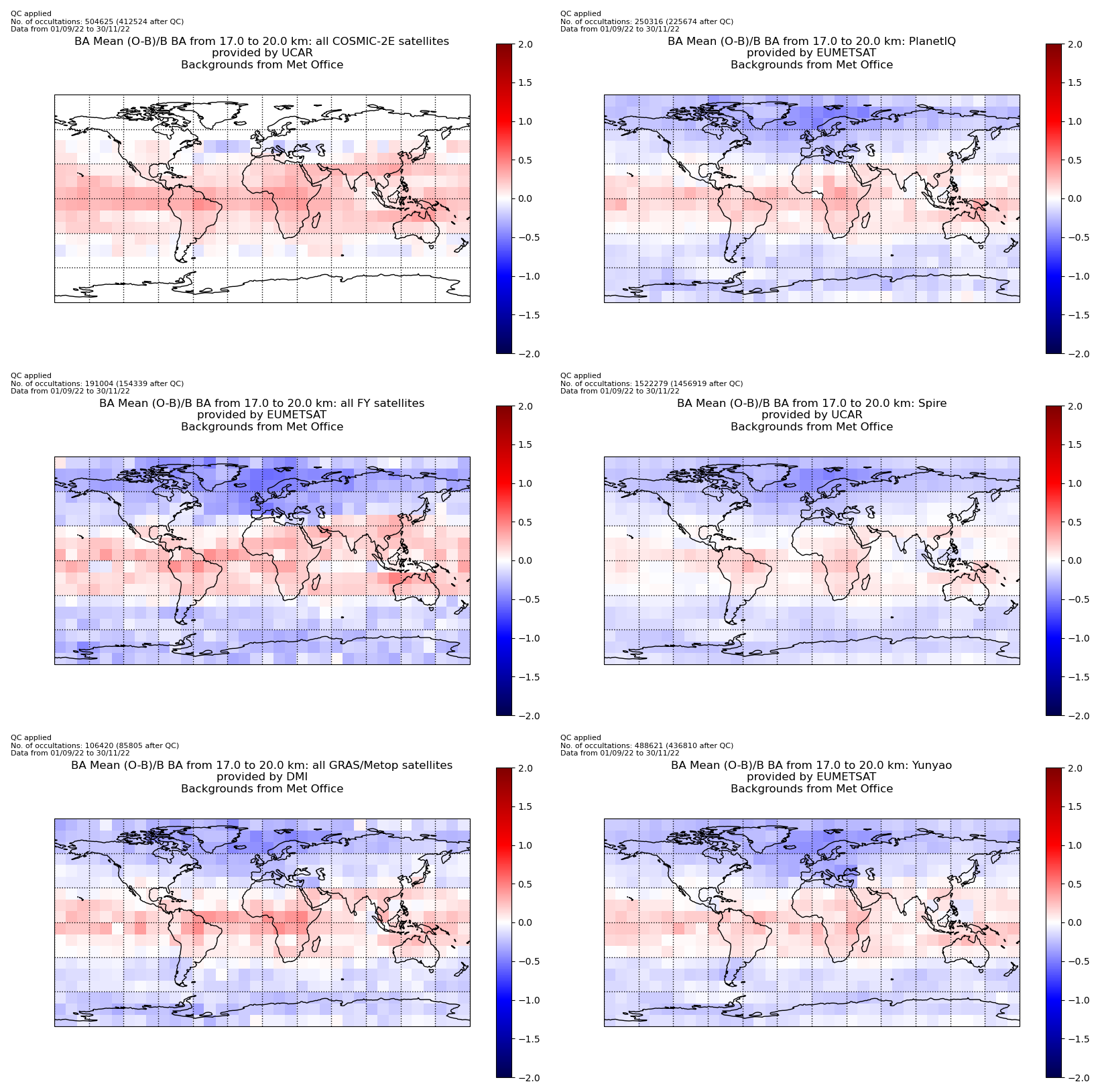
Figure 14 Mean difference between the observations and the model background of the observations, normalised by the model background. The data are averaged over all the ROMEX observations, but binned by latitude and longitude.

One further way to understand the spatial variation of the bias is to examine the spatial distribution of the O−B statistics. Figure 14 shows the mean values of $(O-B)/B$ (note: not $(O-B)/\left(\mathrm{0.5}\right(O+B\left)\right)$ as before), averaged over 10 degree bins for various satellite groupings, within the vertical range 17 to 20 km impact height. This impact height range is chosen, as it is in the stratosphere at all latitudes, and experiments have shown that the lower stratosphere is where GNSS-RO observations have most impact since their errors are often smallest in this region (Kursinski et al., 1997). For all of the observation groups it will be noted that a positive O−B is seen in the tropics, and a negative O−B in the mid-latitudes. This is consistent with the results shown in Fig. 13. Little of the negative region is seen for COSMIC-2 observations, since they are in a low-inclination orbit. It is notable that the statistics for FY-3 satellites are slightly more negative than the others in the northern extra-tropics, and that the FY-3 and Metop satellites are slightly more positive than the others in the tropics.

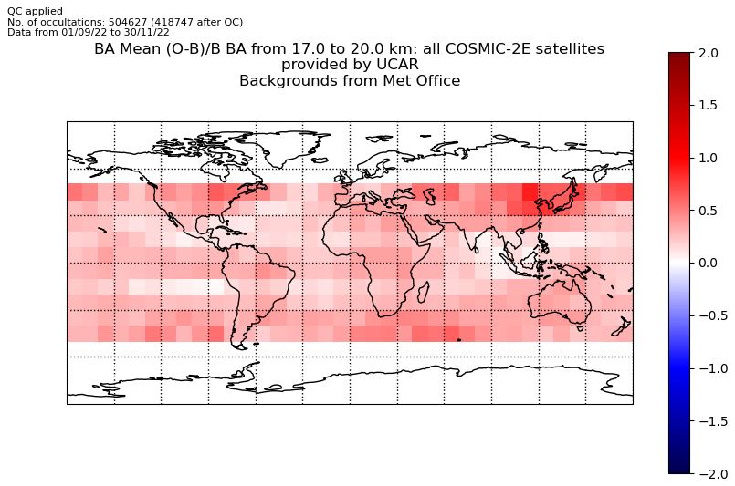
Figure 15 Mean difference between the observations and the model background of the observations, normalised by the model background. Calculated within a system which does not account for tangent-point drift using COSMIC-2 observations. The data are averaged over all the ROMEX observations, but binned by latitude and longitude.

Figure 14 was calculated using the monitoring software that the Met Office has developed for the ROM SAF¹. It was recently noted that this software did not account for the drift in the tangent point when calculating the background bending angles. Whilst Fig. 14 was calculated without this deficiency, the following NWP tests were based on bias estimates which included this defficiency. It makes little difference to the bias estimates, because the observations are made at a variety of azimuth angles, leading to a cancellation of biases. The one exception to this are the COSMIC-2 satellites; the observations made at higher latitudes share a similar geometry, with the occultation being aligned approximately north-south. This leads to a systematic shift in the bias estimates. Figure 15 shows the bias estimates from COSMIC-2 when tangent-point drift is not accounted for. It is clear that these estimates are systematically more positive. It should be noted that whilst the bias estimates were calculated in a system which didn't account for tangent-point drift, it was implemented into a data assimilation system which does, and therefore the benefit of COSMIC-2 observations within these tests may be diminished.

3.1 Attempts to apply spatially varying bias correction

Given the latitudinal and longitudinal variation in the O−B statistics, it is possible that a spatially varying bias correction could be applied to the observations. This may be able to account for the variation in bias between the different observation groups, but also for the strong variation of the bias with latitude. To test this hypothesis, the bias statistics were calculated in 30° latitude/longitude bins, and the mean statistics of $(O-B)/B$ were calculated for each of the observation groups shown in Fig. 14. The statistics were calculated using the following height bins: 2–5, 5–8, 8–12, 12–17, 17–20, 20–25, 25–30, 30–35, 35–40, 40–45, 45–50, 50–55 and 55–60 km impact height. Once these statistics were calculated they were used as the basis for the bias correction. When the observation were ingested, the latitude, longitude and impact height was compared with the bin centres, and the mean $(O-B)/B$ statistics were linearly interpolated to the observation locations. The observations were then bias corrected using these statistics. Thus, if the mean $(O-B)/B$ statistics were equal to 0.01 at the observation location, then the observation was multiplied by 0.99 (i.e. a positive $(O-B)/B$ indicates that the observation needs to be reduced). In this experiment we are correcting the observation for the apparent bias – irrespective of whether that bias is due to the observations or the model background.

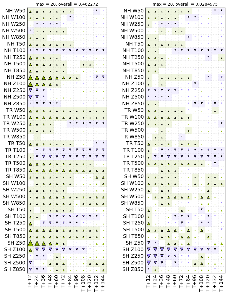
Figure 16 Scorecard showing the change in root-mean-square forecast error for the experiment with all ROMEX observations but with a spatially varying bias correction, compared to the control. Figure format as in Fig. 1.

Figure 16 shows the results of this experiment. Unlike the experiments which alter the refractivity coefficients, this experiment displays improved scores for geopotential height forecasts at 50 and 100 hPa in the northern extra-tropics when verified against ECMWF analyses. This would suggest that the bias correction at high altitudes is somewhat different to the effect of changing the coefficients. However, the RMSE for the tropospheric geopotential height forecasts are increased, suggesting that the bias correction is not performing as well as the refractivity coefficient changes. Whilst the overall score for verification against ECMWF analyses is approximately as good as the overall score when changing both the k₁ and k₂ coefficients, the RMSE against observations is worse. This suggests that the spatially varying bias correction is not as effective as the refractivity coefficient changes, but may provide useful effects at high altitudes.

4 Impact of increasing the number of observations

The stated aim of the ROMEX project is to quantify the benefits of increasing the volume of RO observations by incorporating additional data not currently available to weather centres for real-time operational systems. Therefore, it is good to assess how the quality of the NWP forecasts changes with the number of observations. If we were to perform this assessment using the unadjusted operator, then we would be measuring the degradation brought by the increase in the number of observations. Hence, the above corrections to the system are necessary to demonstrate the benefit which can be achieved using a well-calibrated system.

Following discussion, the following experiments have been run:

• No GNSS-RO observations

• The ROMEX control, but excluding observations from the COSMIC-2 satellites

• The ROMEX control

• A selected set of observations, with around 20 000 occultations per day

• All ROMEX observations

This set of experiments covers a wide range of observation numbers, which should therefore demonstrate a wide range of behaviour. Experiments were run with each of these datasets, using a modified version of the operator. The modifications to the operator are to reduce k₁ by 0.05 % and k₂ by 3.5 %, as described earlier. In addition to this, a vertical smoothing of the observations within a profile is applied where the smoothing length-scale is approximately $\mathrm{3}/\mathrm{4}$ the model-level spacing, as described in Bowler and Marquardt (2026). Finally, a simple bias correction is applied to high-altitude observations. For this, we define latitude regions of 0–30, 30–60 and 60–90° away from the equator, and calculate approximate bias corrections for each region. The bias correction within 10° of each region boundary is linearly interpolated and is applied as a multiplicative factor to the observed bending angles. Within the tropics the bias correction decreases linearly from 1 (no correction) at 36 km to 0.988 at 48 km, and then back to 1.0 at 60 km. Between 30 and 60° (north and south) the bias correction factor decreases linearly from 1 at 34 km to 0.985 at 46 km and stays at this value above this height. Above 60° the bias correction factor decreases linearly from 1 at 35 km to 0.983 at 45 km, and stays at this value above this height.

The measured bending angle bias at high altitudes is different between the ECMWF and Met Office systems. The Met Office system has a positive bias at high altitudes, whereas the ECMWF system's observed bias is closer to zero. One feature of the Met Office system is that the forward operator doesn't ingest the forecast temperature directly. Instead it is provided with the air pressure and specific humidity, and the virtual temperature is derived from these. We conducted a very brief experiment in which we altered the operator to work directly from the temperature provided by the model. This reduced the bias at high altitudes, bringing the statistics much closer to those of ECMWF (not shown). Therefore, applying this bias correction to the observations is unjustified since we are correcting the observations to look more like the model. However, applying a bias correction at high altitudes appears to be effective at improving the forecast quality, and therefore it is included in the experiments.

The dataset with 20 000 occultations per day was provided by EUMETSAT. This dataset included the following satellites and satellite constellations: COSMIC-2, Metop, TanDEM-X, TerraSAR-X, Sentinel-6A, PlanetIQ and Spire. The individual Spire satellites were chosen each day to provide a total of approximately 20 000 occultations, after quality control has been applied. Thus, there were more than 20 000 occultations each day in this dataset.

4.1 Trial results

Figure 17 shows the results of an experiment with all ROMEX observations, using the modified operator described above. The results are broadly similar to the experiment with altered refractivity coefficients (Fig. 8), but with a few notable differences. The improvements when verifying against ECMWF analyses are generally larger, such as the short-range forecasts in the tropics. Unfortunately, some scores are also degraded, such as the temperature at 100 hPa in the medium range. Nonetheless, this configuration was deemed to be the best performing of all the experiments, and therefore was used for the tests of the impact of increasing the number of observations.

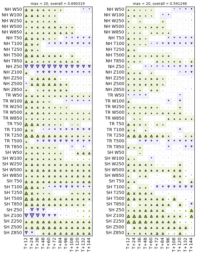
Figure 17 Scorecard showing the change in root-mean-square forecast error for the experiment with all ROMEX observations but with a modified operator which uses altered refractivity coefficients, vertical smoothing of the observations and a bias correction at high altitudes, compared to the control. Figure format as in Fig. 1.

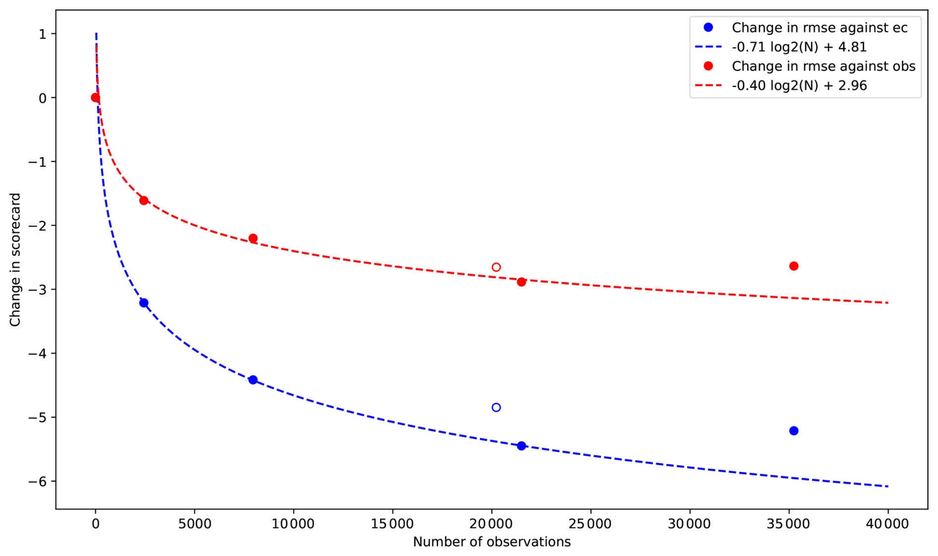
Figure 18 Average percentage reduction in RMSE across scorecard variables and lead times for the different experiments. Verification against ECMWF analyses is shown in blue, and verification against observations is shown in red. A best-fit curve based on a variation of the overall figure with the logarithm of the number of observations is shown as the dashed line. The curve has been fit to the experiments using Control – COSMIC-2, control, and 20 000 occultations per day. The number of observations shown is an approximate figure calculated before quality control. The hollow circle indicates the results from the alternative 20 000 occultations per day experiment.

To compare the impact of the number of observations on the forecast quality we use the overall figure from the scorecard. This is the average of the change in RMSE for all the variables and lead times shown in the scorecard. No weighting is given, so the individual components are treated equally. Figure 18 shows the change in the overall value for the RMSE scorecard for the different experiments. The results fit well to a logarithmic dependence of the overall forecast quality varying with the number of observations, as was proposed by Bowler (2020a). However, it will be noted that the forecast quality is lower for the experiment with all ROMEX observations than for the experiment with 20 000 occultations per day.

The apparent degradation when assimilating all the observations caused some confusion. However, we noted that the 20 000 occultations per day dataset is not a random sampling of the full dataset, but excludes certain satellite constellations. It excludes observations from the following satellites and satellite constellations: FY-3, Tianmu, Yunyao, KOMPSAT-5 and GeoOptics. Therefore, if observations from these satellites are less beneficial, or even harming the forecast quality then we would expect the 20 000 occultations per day dataset to be the best performing. Separate experiments testing the assimilation of FY-3E into our operational environment showed a degradation in performance (Lewis, 2025). Therefore, we speculate that different observations are of different quality (such as different local time sampling and processing differences) and that the 20 000 occultations per day dataset kept those which are most beneficial to the Met Office's NWP system. However, it should be noted that during January 2025 the Chinese Meteorological Administration introduced an update to their processing of Fengyun observations, which appears to have led to substantial improvements (Yan Liu, personal communication, 2025).

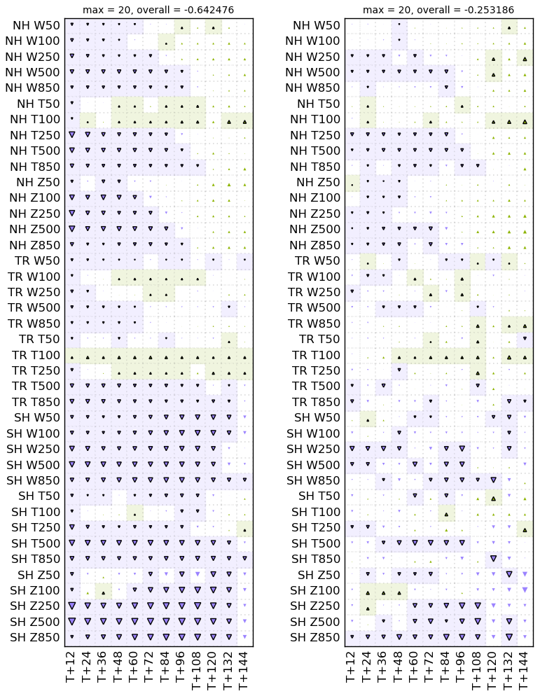
Figure 19 Scorecard showing the change in root-mean-square forecast error for the experiment using the alternative 20 000 occultations per day dataset, compared with the EUMETSAT 20 000 occultations per day dataset. Both experiments used the modified operator which uses altered refractivity coefficients, vertical smoothing of the observations and a bias correction at high altitudes. Figure format as in Fig. 1.

To test the hypothesis that different satellites provide different levels of benefit, a further experiment was run creating an approximately 20 000 occultations per day dataset, but with a different mix of satellites. This experiment used observations from the following satellites and satellite constellations: COSMIC-2, FY-3, Metop, KOMPSAT-5, PAZ, PlanetIQ, Sentinel-6A, TanDEM-X, TerraSAR-X, Yunyao and Spire (flight-model numbers 150, 162 and 163 only). Note that this dataset has slightly fewer observations at 20 223 observations per day, compared to 21 496 observations per day for the EUMETSAT dataset. Figure 19 shows the scorecard for this experiment, compared against the experiment with the EUMETSAT dataset. There are clear degradations in many quantities for using the alternative dataset, especially at short range in the southern extra-tropics. Therefore, it seems that the quality of the observations being used is important, and not simply the quantity.

4.2 Data assimilation statistics

Given that we see no further improvement in the RMSE scores with the addition of more observations beyond the official 20 000 occultations dataset, it is interesting to consider whether this is also seen in the data assimilation statistics. Since a 6 h data assimilation window is used, the background forecast lead time is between 3 and 9 h. Figure 20 shows the ratio of the standard deviation of the difference between the observations and model background for the different experiments, relative to the test without GNSS-RO observations, as a function of the number of observations. For all groupings of the observations, the use of GNSS-RO observations improves the fit of the model background to the observations. The amount of improvement depends on the observation type being considered, which may reflect the level of noise intrinsic to the observations. The biggest reduction in standard deviation is seen for radiosonde potential temperature, which is improved by up to 4 % with the addition of GNSS-RO observations. This is the only observation type for which the all-observations experiment performs better than the 20 000 occultations per day experiment, although this difference is not statistically significant. The other observation types appear to show that the all observations experiment performs worse than the 20 000 occultations per day experiment, consistent with the overall forecast results.

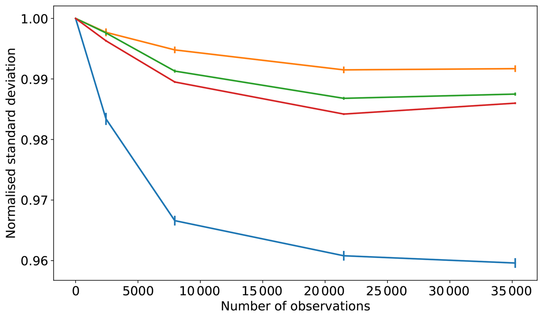
Figure 20 Ratio of the standard deviation between the observations and model background for the different experiments, relative to the experiment with no GNSS-RO observations, as a function of the number of observations. Shown are the statistics for upper-levels winds (orange, taken from aircraft, sonde and atmospheric motion vectors), microwave radiances (green, aggregated from ATOVS on Metop-B/C, NOAA-15/18/19, and ATMS on JPSS and NOAA-20), hyperspectral infrared radiances (brown, taken from IASI on Metop-B/C and CrIS on JPSS and NOAA-20) and potential temperature from radiosondes (blue). The number of observations shown is an approximate figure calculated before quality control. Note that the 20 000 occultations per day experiment shown here is the default one provided by EUMETSAT.

4.3 Which variables are driving behaviour?

Since we are noting that the Met Office system gains little additional benefit from the full set of observations due to the final set of observations being less beneficial in the Met Office system, it is interesting to consider which variables are driving the behaviour. Figures 21 and 22 show the change in RMSE for the different variables in the various latitude regions, as a function of the number of observations. For verification against sonde observations (Fig. 21), the RMSE in the southern extra-tropics for the all-observations experiment decreases much more than for the other regions. For the northern extra-tropics there is very little additional benefit for the addition of observations above the baseline which excludes COSMIC-2 observations. For the tropics, the RMSE reduction continues with the inclusion of COSMIC-2 observations, and shows limited improvements thereafter. For the southern extra-tropics the reduction in RMSE continues up to 20 000 occultations per day, but then increases with the addition of all ROMEX observations. Therefore, it is likely that the southern extra-tropics is driving the degraded performance with all ROMEX observations, but that the other regions mostly saturate at a lower number of observations.

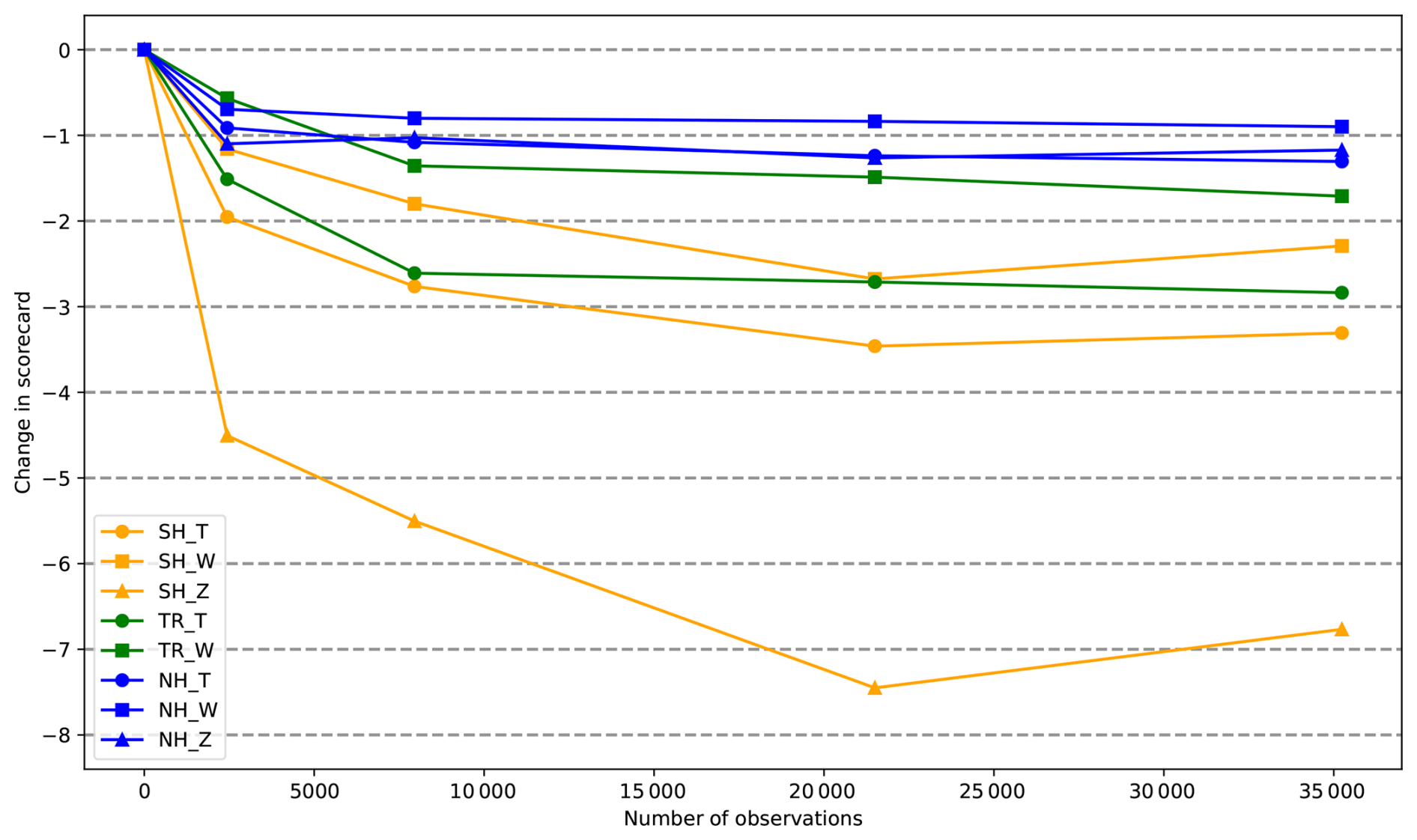
Figure 21 Average percentage reduction in RMSE across scorecard variables and lead times as a function of the number of observations for variables in different latitude regions. Verification against sonde observations. The number of observations shown is an approximate figure calculated before quality control. Note that the 20 000 occultations per day experiment shown here is the default one provided by EUMETSAT.

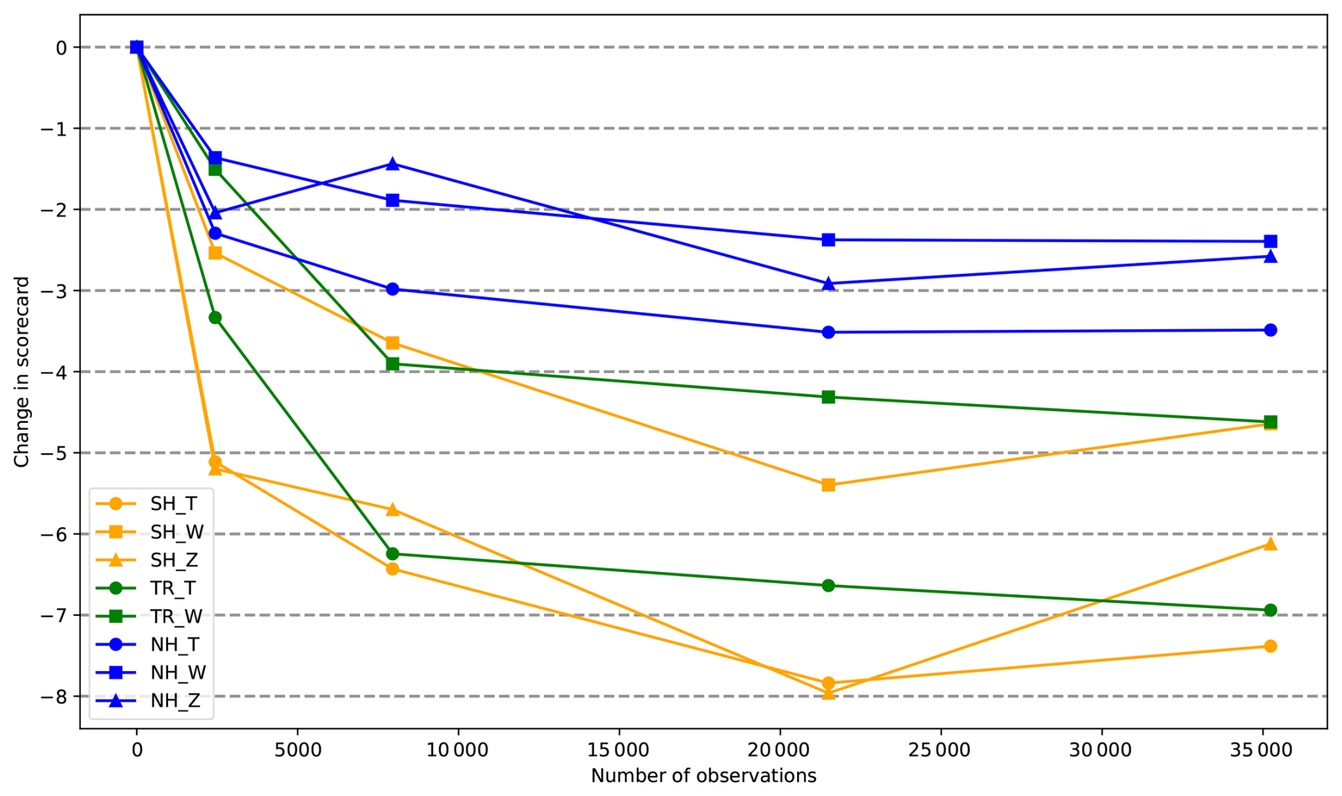
Figure 22 Average percentage reduction in RMSE across scorecard variables and lead times as a function of the number of observations for variables in different latitude regions. Verification against ECMWF analyses. The number of observations shown is an approximate figure calculated before quality control. Note that the 20 000 occultations per day experiment shown here is the default one provided by EUMETSAT.

When verifying against ECMWF analyses (Fig. 22), the RMSE reduction is more uniform across the different latitude regions. Whilst the rate of improvement in the RMSE scores decreases with an increasing number of observations, the RMSE scores are improved in the tropics and northern extra-tropics with all ROMEX observations, relative to the 20 000 occultations per day dataset: there is no sign of saturation of benefit in the addition of observations. This is not the case for the southern extra-tropics, where the RMSE scores are degraded with the addition of all ROMEX observations. Looking at the individual scorecards (not shown) the degradation in RMSE scores in the southern extra-tropics cannot be ascribed to a single variable or lead time, but instead is the combined effect of slight degradations in all variables and lead times.

There are many possible reasons which could lead to the differences noted above in the verification against sondes and ECMWF analyses. It seems likely that the location and density of the verifying data points is an important factor. Sondes in the northern extra-tropics are concentrated over land, and particularly over Europe. This is a very well observed region which benefits less from additional observations. Verification against ECMWF analyses is performed on a 1.5 degree regular grid, with a weighting using the cosine of the latitude. This means that these results will be sensitive to changes in performance over the oceans as well as over land. Since the oceans are less well observed, the additional GNSS-RO observations are likely to be more beneficial.

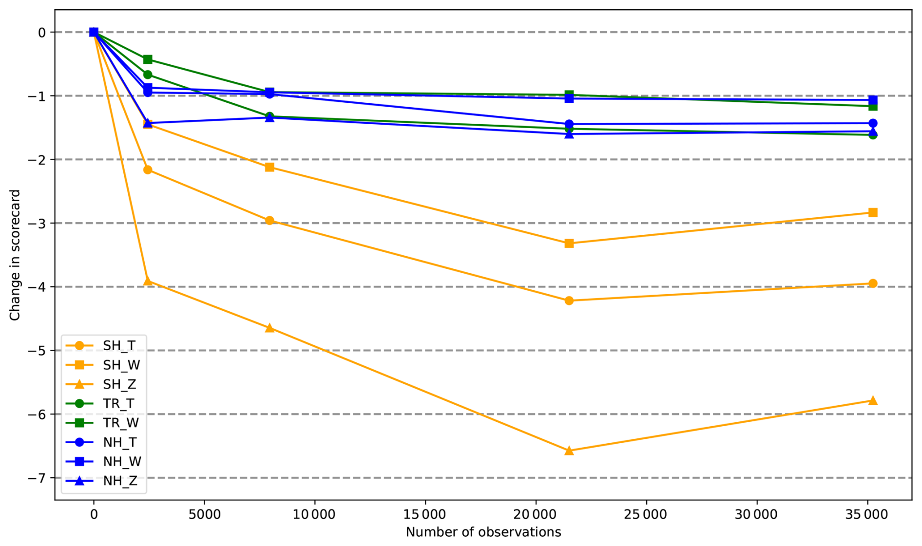
Figure 23 Average percentage reduction in RMSE across scorecard lead times and variables at 850, 500 and 250 hPa as a function of the number of observations for variables in different latitude regions. Verification against sonde observations. The number of observations shown is an approximate figure calculated before quality control. Note that the 20 000 occultations per day experiment shown here is the default one provided by EUMETSAT.

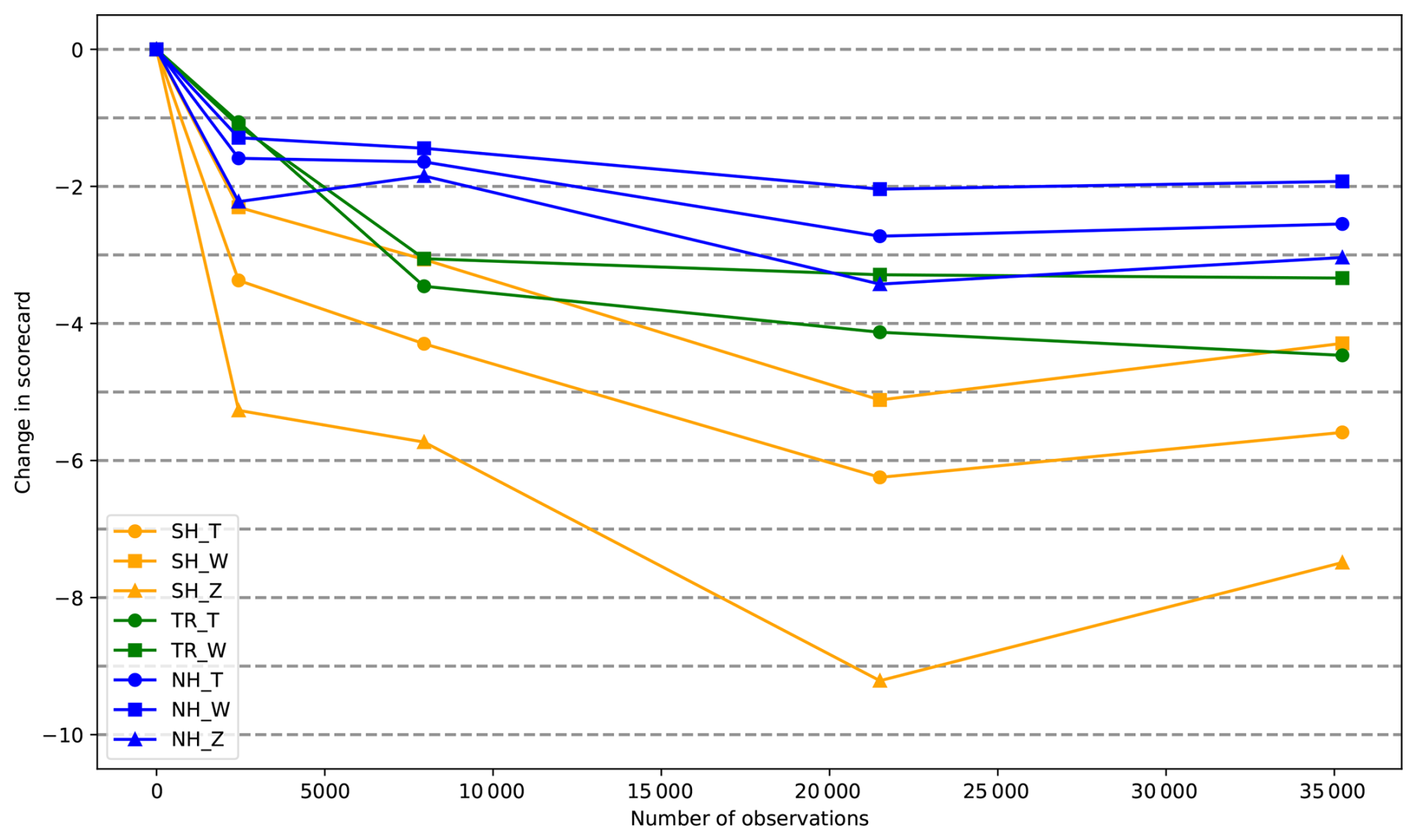
Figure 24 Average percentage reduction in RMSE across scorecard lead times and variables at 850, 500 and 250 hPa as a function of the number of observations for variables in different latitude regions. Verification against ECMWF analyses. The number of observations shown is an approximate figure calculated before quality control. Note that the 20 000 occultations per day experiment shown here is the default one provided by EUMETSAT.

Another factor is the behaviour of the forecast in the troposphere and at higher altitude. Figures 23 and 24 show the change in RMSE, like Figs. 21 and 22, but only considering variables at 850, 500 and 250 hPa. For these lower-altitude quantities the benefit from additional GNSS-RO observations appears to continue to higher observation numbers. This is because the alterations to the refractivity coefficients have been effective at correcting the bias problems at these altitudes, whereas the bias problems at higher altitudes are not so well corrected. When verifying against observations (Fig. 23), there is still early saturation of benefit in the northern extra-tropics. However, in the tropics there is no sign of saturation. When verifying against ECMWF analyses (Fig. 24) the benefit in the northern extra-tropics appears to saturate at 20 000 occultations per day, but no saturation is seen in the tropics. In both cases the behaviour in the southern extra-tropics is similar to that seen in the full RMSE scorecard, with a degradation in performance with the addition of all ROMEX observations.

5 Conclusions

The ROMEX set of experiments have aimed to demonstrate the benefits to NWP from the use of additional GNSS-RO observations. Unlike previous studies which have used synthetic observations, the ROMEX project has used real observations from a variety of satellites and satellite constellations. On the one hand, the results are more trustworthy because they are based on real observations. On the other hand, the tests have highlighted issues with the use of the observations, and the need to adjust the observation operator to account for forecast biases which have appeared from the use of the observations.

The initial experiments with the additional observations showed an increase in the RMSE of forecast error. The degradation was particularly clear for tropospheric geopotential height forecasts, which was shown to be largely due to a forecast bias. Various experiments were run exploring the effect of bias corrections to the observations, and changes to the coefficients of the refractivity operator, which achieve a broadly similar effect. It was found that the bias in tropospheric geopotential height forecasts is largely controlled by observations in the lower stratosphere, and small changes to the refractivity coefficients in the observation operator are able to control this. Experiments within a 1D-Var framework demonstrated that the change in geopotential height biases are largely due to pressure increments from observations centred around 15 and 10 km impact height. The global average difference between the observations and background forecast in the lower stratosphere is around 0.05 %, which leads to a suggestion that this might be an appropriate adjustment to make to the dry refractivity coefficient.

Following these experiments it was found that changes to both the k₁ and k₂ coefficients in the refractivity operator performed best, although neither change has a clear theoretical justification. It was decided to reduce k₁ by 0.05 % and k₂ by 3.5 %. This was shown to be effective in reducing the forecast bias, and improving the forecast quality, except when verifying geopotential height forecasts at 50 hPa against ECMWF analyses. Therefore, these changes were used in the final experiments. Other centres have shown similar levels of bias when assimilating the full set of ROMEX observations. However, whilst the Met Office forecasts were degraded by this bias, both when verifying with the RMSE and the standard deviation of forecast error, other centres found that the standard deviation of forecast error was reduced when assimilating the additional observations, with or without changes to the refractivity coefficients. It is not clear why the Met Office stands out as being particularly negatively affected by the bias changes.

The apparent bias between the observations and the model background varies spatially, in all three dimensions. The apparent bias is largely similar between different groups of observations, which may suggest that the biases are dominated by model errors rather than deriving from the observations. Applying a spatially-varying bias correction to the observations, based on the measured apparent bias was attempted. This proved to be effective in many respects, particularly when verifying against ECMWF analyses. However, the overall performance was not as good as the refractivity coefficient changes, and therefore this approach was not pursued further.

For the final experiments a configuration was chosen which used adjusted values of the refractivity coefficients, applied a latitude-dependent bias correction for observations at high altitude (to correct for large model biases in this region), and used a vertical smoothing of the observations. With these settings, experiments were run with a varying number of observations. It was found that the overall RMSE scores improved with increased numbers of observations, up to a maximum of 20 000 occultations per day. Beyond this point, the RMSE scores were slightly degraded, particularly in the southern extra-tropics. It was found that the 20 000 occultations per day dataset preferentially removed certain satellites and satellite constellations. Some of these satellites have been shown independently to be less beneficial to the NWP forecasts from the Met Office, and therefore the particularly good performance of the experiment with the 20 000 occultations per day dataset is likely due to its inclusion of only satellites which are highly beneficial in the Met Office system. When splitting the results by latitude region, it was found that the southern extra-tropics was driving the degradation in performance with the addition of all ROMEX observations.

It should be noted that the benefit of the additional GNSS-RO observations was only demonstrated in the Met Office system once the adjustments to the refractivity operator were made, correcting the forecast bias that was apparent. Experiments with a more sophisticated derivation of the refractivity operator were not conducted. However, similar experiments made at other centres demonstrated similar changes in the bias, and therefore it is not guaranteed that a different operator would yield different results. The appearance of these issues only occured because the experiments used real, rather than synthetic, observations, which demonstrates the value of using real observations in the experiments.