Spatio-temporal pattern analysis of MOPITT total column CO using varimax rotation and singular spectrum analysis

In this paper, we apply varimax Empirical Orthogonal Function (EOF) analysis to Measurement of Pollution in the Troposphere (MOPITT) total column CO retrievals to answer the question of whether or not it is possible to disentangle the dominant CO sources associated with inferred modes of variability at regional to global scales. This study aims to highlight the strengths and limitations of EOF analysis, specifically their usage in the field of atmospheric chemistry. In particular, we highlight an instance where varimax rotation fails to reveal additional spatial structure of a dataset. Additionally, we emphasize to the reader that the success of EOF analysis to determine linearly independent physical modes relies on both the statistical distribution of the dataset as well as its temporal covariance structure. We analyzed daily MOPITT Version 8 Level 3 joint (TIR-NIR) products from 2005 to 2018, aggregated every 8 d on a 1° by 1° grid. Our findings show that EOF patterns of MOPITT CO are consistent across various regional subdomains, demonstrating that these spatial patterns are independent of the chosen domain. A comparison of the eigenvalue spectrum reveals that unrotated EOF analysis yields three distinct modes, while varimax rotation reduces these to two. The power spectra of the principal components indicate that the first two unrotated modes are primarily driven by annual and semi-annual cycles, while the third mode reflects seasonal variations occurring over roughly three months. To further isolate these modes, we employed singular spectrum analysis (SSA) at each grid point to generate long-term, seasonal, and residual EOF patterns. The power spectrum analysis of the principal components shows that the long-term EOFs replicate the original two dominant modes, while the seasonal EOFs reveal significant variations over 2 to 3 months, and the residual modes exhibit time scales of 2 months or shorter. By plotting the mean skewness field, we show the dataset is non-Gaussian, leading us to conclude its principal components are time-dependent despite being uncorrelated. The periodic decay observed in the temporal autocorrelation function for each time series suggests a classification of wide-sense cyclostationary behavior. The non-stationarity of each time series and the temporal dependence of modes lead us to conclude that EOF analysis alone cannot fully disentangle individual CO sources. Careful consideration is therefore required when interpreting EOF patterns of other composition datasets with similar characteristics.

1 Introduction

The Role of Carbon Monoxide in Atmospheric Composition

Carbon monoxide (CO) plays an important role in tropospheric chemistry and composition. Firstly, its reaction with the hydroxyl radical (OH) has a significant impact on the atmospheric oxidizing capacity. CO as well as non-methane volatile organic compounds (NMVOCs) are both responsible for positive climate forcing because they raise tropospheric ozone (O₃) and methane (CH₄) by creating a global sink for OH (Fiore et al., 2012). The spatiotemporal variations in CO (and hence OH) can lead to changes in O₃ abundance depending on whether the concentration of nitrogen oxides (NO_x) is low or high (Sillman et al., 1990; Jin et al., 2017). Regions of high NO_x experience O₃ production while clean areas with low NO_x experience the destruction of O₃ (Holloway et al., 2000). Because OH is a photochemical sink of CO through oxidation, its global distribution determines the lifetime of CO and therefore, values of CO are lowest with the shortest lifetime in regions with the highest OH. Secondly, CO can also serve as a tracer of pollution transport given its medium-length lifetime (weeks to months) (Cicerone, 1988). Mainly a product of incomplete combustion of wood and fossil fuels, CO is co-emitted with nitrogen dioxide (NO₂), black carbon (BC), and carbon dioxide (CO₂). It is more concentrated in the atmospheric boundary layer (with less in the stratosphere) so observing CO can be useful as well to study the exchange of these gases and aerosols across the troposphere. Because CO is the main sink of OH (Gaubert et al., 2020), it is important for quantifying losses of CH₄ in the troposphere as well (Myhre and Shindell, 2014; Gaubert et al., 2016, 2017; Nguyen et al., 2020). The lack of constraints on OH spatiotemporal variability as well as the interannual variability of CH₄ have both made it difficult to accurately determine the global CH₄ budget (Saunois et al., 2016; Turner et al., 2019; Prather and Holmes, 2017). This means there is a need to reduce the uncertainty of primary drivers of OH, including CO, O₃, H₂O, NO_x, and NMVOCs (Gaubert et al., 2020).

Determining the spatial and temporal distribution of CO, along with the distribution of co-emitted species including NO₂, CO₂, CH₄ and aerosols, helps us to understand trends of combustion, biomass burning, and other sources of air pollution. For example, Lin et al. (2020b) uses a combined mean and standard deviation approach for total column CO to classify local regions of Southeast and East Asia based on combustion activity into areas of intense urbanization, large-scale biomass burning, regions undergoing significant change from one type to another, and clean regions. Raman and Arellano (2017) utilized variations in enhancement ratios of elemental carbon (EC), CO, and NO₂ to investigate processes driving EC levels across the United States. Tang and Arellano Jr. (2017) demonstrated that local enhancement ratios of $\mathrm{\Delta }\mathrm{CO}/\mathrm{\Delta }{\mathrm{NO}}_{\mathrm{2}}$ can distinguish different combustion types, identifying whether or not a fire was in a flaming phase or smoldering phase while Silva et al. (2013) used $\mathrm{\Delta }\mathrm{CO}/\mathrm{\Delta }{\mathrm{CO}}_{\mathrm{2}}$ to identify combustion efficiency patterns in urban agglomeration. Building on this, Silva and Arellano (2017) combined $\mathrm{\Delta }\mathrm{CO}/\mathrm{\Delta }{\mathrm{CO}}_{\mathrm{2}}$ and $\mathrm{\Delta }\mathrm{CO}/\mathrm{\Delta }{\mathrm{NO}}_{\mathrm{2}}$ to better characterize regional-scale combustion process while Tang et al. (2019) used $\mathrm{\Delta }\mathrm{CO}/\mathrm{\Delta }{\mathrm{NO}}_{\mathrm{2}}$ and $\mathrm{\Delta }\mathrm{CO}/\mathrm{\Delta }{\mathrm{SO}}_{\mathrm{2}}$ to track the common combustion emission pathways across China. Recently, Mottungan et al. (2024) demonstrated the value of multi-species enhancement ratios (CO, CH₄, CO₂) along with multivariate regression methods to differentiate between regional and local influences, and identify the dominant processes driving these patterns.

However, determining accurate trends in air pollution is difficult in practice for many different reasons. While there has been an increasing availability of satellite measurements of trace gases and aerosols in the recent decade, most of these remote sensing retrievals cannot, in general, tell us where their source or sink was due to the diffusive nature of atmospheric transport (Murayama et al., 2004). Another challenge is that space-based CO measurements often lack accuracy in areas with persistent cloud cover and near the surface, where thermal infrared sensors struggle due to interference from surface radiation and limited retrieval sensitivity (Clerbaux et al., 2008). These significant sources of uncertainty require us to cross-validate satellites across different instruments as well as with ground and aircraft measurements during field campaigns, and are especially problematic over areas such as Sub-Saharan Africa, where there are very few air quality monitoring stations (Malings et al., 2020; Gualtieri et al., 2024). Determining the background value of constituents is especially difficult on a global scale because it changes across time and space based on the sources and sinks for a given region and chemical regime (Jones et al., 2003; Wang et al., 2018; Borsdorff et al., 2019). Because satellites measure the total amount of a constituent rather than the source of emission for a given region, it is difficult to tell whether local changes in the overall trend are due to anthropogenic or biogenic sources or the background or residual burden (Novelli, 1999; Tang et al., 2022). As discussed in Buchholz et al. (2021) there are no overall trends in either CO or aerosol optical depth (AOD) in Central/Southern Africa despite the increasing trend in anthropogenic combustion in Central Africa as determined by Zheng et al. (2019) which may be counteracting the global decrease in CO. Buchholz et al. (2021) have also noted that the increase in burning in the region as shown in Andela et al. (2017) may be potentially counteracting transport.

There are several complex challenges when determining emission inventories. As discussed by Gaubert et al. (2020), emission inventories in China are low in comparison to in situ observations in the case of both forward and inverse models, and in particular there is an underestimation of CO despite having revised inventories (Li et al., 2017; Feng et al., 2020; Kong et al., 2020) as explained by an underestimation of residential coal combustion from either heating or cooling (Chen et al., 2017; Cheng et al., 2017; Zhi et al., 2017). Even though this underestimation of fossil fuel burning does explain the underestimation of Northern Hemisphere (NH) CO in global models (Shindell et al., 2006), this is confounded by the large difference in modeled variability of the regional distributions of OH in the NH, which could offer an alternative explanation (Naik et al., 2013; Young, 2013). Gaubert et al. (2020) used observations from the Korea-United States Air Quality (KORUS-AQ) field campaign to investigate this underestimate over East Asia and found that assimilation of CO improves the representation of OH in global chemical transport models by correcting OH $/$ HO₂ partitioning. This also implies that assimilation of CO should help study coupled CH₄-CO-OH reactions, which allow for chemical feedback. Effectively distinguishing the signature of secondary CO from the influence of surface emissions – whether anthropogenic, biogenic, or from fires – is crucial for enhancing the reliability of source attribution studies, including inverse modeling for air quality assessments and chemistry-climate simulations (Gaubert et al., 2016, 2017; Worden et al., 2019; Gaubert et al., 2020; Miyazaki et al., 2020; Gaubert et al., 2023). This separation also aids in the physical interpretation of observed air pollution patterns, with important implications for understanding the distributions of both OH and CH₄ (Gaubert et al., 2017; Vimont et al., 2019; Hooghiem et al., 2025).

To address some of these challenges, we attempt to answer the following questions in this study:

1. How can we use the spatial and temporal distribution of CO to detect the difference between anthropogenic and natural variability of CO?

2. Can the global background of CO be disentangled from the local-to-regional influences on observed CO abundance?

We use the term “global background” to refer to a mathematical, non-physical quantity broadly represented as an average. This is different from terminology frequently used in literature. For example, Menichini et al. (2007) defines a background concentration as the observed concentration at a site “not affected by local sources of pollution”. More recently, Han et al. (2015) described background concentration as the collective contribution of sources from regional, anthropogenic, natural emissions, and long-range transport.

To attempt an answer to these questions, we use Empirical Orthogonal Function (EOF) analysis, which is a pattern analysis method to determine the dominant spatio-temporal patterns of a dataset (Hannachi et al., 2007). To avoid confusion with language, we clarify that the term EOF analysis refers to the usage of principal component analysis (PCA) (a statistical technique used to reduce dimensionality) when it is applied to the fields of climate science and geophysics. While the two methods are virtually identical, the use of EOF analysis implies that the principal components being found are not just linearly uncorrelated, but they are also being used to explain the maximum amount of variance possible in the original dataset.

EOF analysis has been extensively utilized in climatology, for instance Wallace and Gutzler (1981) performed an EOF analysis of geopotential height to generate what we now refer to as atmospheric teleconnections. It has had fewer applications to atmospheric chemistry, but for instance Li et al. (2009) uses varimax rotated EOF analysis of de-seasonalized aerosol index to isolate major dust and biomass burning regions and dust transport. Li et al. (2013) performed a similar analysis on AOD datasets. Lin et al. (2020a) also verified the result of their classification of urban and biomass burning regions using EOF analysis. Yin et al. (2019) used EOF analysis to analyze the dominant patterns in summer O₃ pollution over Eastern China and their relationship to atmospheric circulations. EOF analysis has also seen applications to air quality monitoring. For instance, Eder et al. (1993) uses the principal components corresponding to rotated modes to analyze seasonality of surface ozone concentrations in the Eastern United States. Pires et al. (2008) used principal component analysis together with cluster analysis to examine monitoring sites and identify emission sources as well as cities with similar pollution behavior. They successfully applied this method to several species, including CO, O₃, and NO₂.

Our use of EOF analysis is especially motivated by studies that investigate the global CO budget through source attribution, for example, see e.g. Granier et al. (1999); Holloway et al. (2000); Duncan et al. (2007); Zheng et al. (2019); Lichtig et al. (2024). Holloway et al. (2000) used three-dimensional-modeled CO to study the total CO budget by simulating the tagged contributions from fossil fuel, biomass burning, methane oxidation, and biogenic sources. In doing so, Holloway et al. (2000) was able to reproduce global patterns in the CO seasonal cycle, most importantly the interhemispheric gradient observed in total CO measurements. The same gradient was also detected in the fossil fuel tag, which showed that the global CO seasonal cycle can be thought of as a convolution of the seasonal cycles for individual source terms. Our approach in this study is similar; however, we begin with satellite-based total column CO to separate it into patterns that represent the variability of its individual sources and sinks. This is precisely the class of problem that EOF analysis was designed to solve. Our focus in this paper is to explore the use of EOF analysis on satellite data of atmospheric composition in an attempt to separate anthropogenic and biogenic modes of variability from a global background field. Our results find that while EOFs have proven useful in climatological studies before, using it on atmospheric composition has significant limitations that require careful considerations, as detailed in our study.

2 Data and Methods

2.1 Total Column CO from MOPITT

We use total column CO data from the Measurements of Pollution in the Troposphere (MOPITT) instrument, which uses a correlation radiometer from the NASA Terra instrument. Terra flies at a normal altitude of 705 km in a Sun-synchronous polar orbit that passes over the equator at approximately 10:30 and 22:30 local time. The temporal resolution is daily, which has been averaged into 8 d periods, and the spatial pixel resolution is 22 km × 22 km at nadir, resampled to 1° from L3 products. The cross-track scanning angle is ±26° and yields a swath of approximately 640 km with global coverage every 3 d.

The radiometer performs gas correlation spectrometry for broadband measurements in thermal infrared (TIR) at approximately 2140 cm⁻¹ and near-infrared (NIR) around 4725 cm⁻¹ (Drummond et al., 2010; Buchholz et al., 2021). This is done by modulating either pressure or length of a correlation cell filled with the gas of the target to determine spectral line differences. The TIR is measured using terrestrial thermal radiation, while the overtone band from NIR is measured from reflected solar radiation and enhances retrievals, especially near the surface. Products are available in thermal infrared only, near-infrared only, or joint TIR-NIR, although NIR signals are only available during the day and over land (Buchholz et al., 2017). For this study, we use Level 3 data using the V8 retrieval algorithm for TIR-NIR. Level 2 and Level 3 products for MOPITT for the V8 retrieval algorithms (and their most recent version, V9) are publicly available through repositories located at https://terra.nasa.gov/data/mopitt-data (last access: 20 November 2025).

The V8 product includes updates to MODIS cloud cover Collection version 6.1, spectral data for H₂O and N₂ as well as aircraft data from NOAA (Deeter et al., 2019). This enables a radiance-based bias correction and accounts for both temporal bias drift and bias as a result of water vapor. Daytime retrievals of total column CO for V8 are stable and have a nominal drift of $-\mathrm{0.015}\pm \mathrm{0.061}\mathit{\%}$ relative to NOAA airborne flask sampling during the MOPITT mission. MOPITT measurements have been verified extensively using cross-validation with other satellites, in-situ measurements at the ground, as well as via aircraft, and more recently through ground-based solar Fourier transform infrared spectrometer measurements (George et al., 2015; Buchholz et al., 2017; Martínez-Alonso et al., 2020).

We note that satellite retrievals of tropospheric CO are also available using a multitude of other instruments, including the Atmospheric InfraRed Sounder (AIRS) onboard Aqua (McMillan et al., 2011), the Tropospheric Emission Spectrometer (TES) on Aura (Rinsland et al., 2006), the Infrared Atmospheric Sounder Interferometer (IASI) on the MetOp platform (Clerbaux et al., 2015), the Tropospheric Monitoring Instrument (TROPOMI) (Borsdorff et al., 2018), and the Cross-track Infrared Sounder (CrIS) (Nalli et al., 2020). These instruments are all sun-synchronous, capable of measuring CO in the infrared region, and have been shown to have consistent hemispheric CO variability when compared to MOPITT CO records from 2002 to 2018 (in the case of CrIS, from 2015 onward) (Buchholz et al., 2021). Because CrIS was launched in October 2011, it does not have a long or consistent enough period of measurement to be suitable for the determination of long-term trends of CO. The same applies to TROPOMI, which was launched in 2017. While CO measurements for IASI-A are long enough to determine trends, they have potential discontinuities since CO retrievals are not done using consistent humidity, temperature, and cloud information (Barret et al., 2025). Measurements from TES may be up to 2 orders of magnitude fewer than other instruments and are more difficult to verify due to not being collocated (Buchholz et al., 2021). Measurements from AIRS have a long and stable enough record for trend determination and have been shown to reproduce trends from MOPITT (Yurganov et al., 2008); however, AIRS uses a cloud-clearing algorithm that increases global coverage at the expense of increasing ground pixel sizes to 45 km × 45 km, resulting in coarser resolution (Cho and Staelin, 2006). Our choice of using MOPITT retrievals is because it has the longest available CO record with a verified history of reliable and stable observations and relatively fine spatial resolution.

2.2 Sources and Sinks of CO

Here, we briefly describe the source categories of CO, which include fossil fuel/biofuel burning, biomass burning, biogenic, non-methane hydrocarbon oxidation, and CH₄ oxidation as summarized in Holloway et al. (2000); Edwards et al. (2004, 2006). Describing these categories is useful because surface emissions of CO can display unique signatures that may be linked to specific spatial and temporal patterns in observed CO abundance.

CO from anthropogenic combustion (fossil fuel/biofuel burning) is much larger in the NH compared to the Southern Hemisphere (SH), which is attributed to significantly more fossil fuel consumption in urban and industrial regions. We consider these areas of high emission to be mostly associated with eastern China, India, the eastern United States, and Western Europe. Historically, eastern China has contributed significantly to anthropogenic emissions (Jia et al., 2024) because of a distinct reliance on coal and biofuel burning (Du et al., 2023; Kao et al., 2024). In recent years, however, China has made significant progress in reducing emissions and improving air quality (Greenstone et al., 2021; Li et al., 2024). This has been the case since 2014 when Premier Li Kequiang declared a “war on pollution”, and implemented widespread changes in regulatory policy (Greenstone et al., 2021).

Biomass burning is largest in the SH and a primary source of CO. Biomass burning consists of burning of savanna, forests, agricultural residue, fuelwood, and animal waste and is most concentrated in tropical and sub-tropical forests and grasslands (Holloway et al., 2000). The largest contributions of fire emissions come from Africa and South America, although fires also occur in Indonesia, the Boreal forests of Canada, Alaska, and Russia, as well as Australia. African NH fires occur in the savanna south of the Sahara Desert and in tropical rainforests north of the equator, while SH fires begin burning in the western portion of the continent near Angola and then spread southeast down the eastern coast. Fires in South America happen on the southern edge of the Amazon rain forest, the cerrado grasslands, and drought-deciduous forests in the south (Edwards et al., 2006). Another distinct feature of CO fire emissions is their timing (Wiedinmyer et al., 2023). While long-term drivers such as land-use and land cover changes, as well as drought conditions, heavily influence fire occurrences, seasonal variations are primarily driven by agricultural burning practices and prevailing weather conditions. The anomalously high CO levels from these fires, coupled with their distinct spatial and temporal variability inherent to biomass burning, provide a more reliable signature for distinguishing fire emissions from other CO sources.

The contribution of CH₄ oxidation, as well as oxidation from non-methane hydrocarbons (NMHCs), represents secondary sources of CO that are most apparent in the SH. Oxidation from CH₄ represents roughly 28 % of the global budget (Folberth et al., 2006) while the biogenic component of NMHCs represents roughly 15 % (Duncan et al., 2007). The oxidation of NMHCs includes a wide variety of constituents, which include isoprene, terpenes, acetone, as well as industrial and biomass NMHCs. Temperature-dependent (Sharkey and Yeh, 2001) biogenic emissions of isoprenes are considered the most dominant hydrocarbon emissions due to their large annual contribution (400–600 TgC globally Arneth et al., 2008) and their high reactivity with tropospheric oxidants (Atkinson, 2000). Isoprenes are volatile organic compounds that are directly emitted by trees and shrubs through their leaves. They are also emitted by animals, including humans, and can be measured through various biological processes, including exhaled breath, perspiration, urine, feces, and tear production (Moura et al., 2023). Terpenes are produced mostly from coniferous forests and are released in higher amounts with warmer weather (Holzke et al., 2006). The largest emissions of hydrocarbons occur in the tropics, which are primarily from isoprene and occur because of the large density of biomass and high temperature conditions. During the NH winter, there is a strong gradient resulting from biogenic emissions that are south of the equator, where the intertropical convergence zone is located, and includes emissions from South America, Southern Africa, and Australia. During the NH Summer, biogenic sources contribute more in the NH, resulting in a weaker but still observable gradient. This gradient is significantly stronger for surface observations but is observable at all levels of the atmosphere (Holloway et al., 2000). CO production from CH₄ oxidation can be observed across the troposphere and tends to be spatially homogeneous given the longer lifetime of CH₄ (≈10 years). It does, however, exhibit some seasonality due to chemical loss with its reaction to OH.

The dominant source of oceanic CO is due to sunlight-initiated photolysis of chromophoric dissolved organic matter (CDOM) in the open ocean (Stubbins et al., 2006). CDOM represents the portion of decaying plants and microbes that absorbs light, degrading into CO and other products in the process. The secondary sources of oceanic CO include dark production (the production of CO from CDOM without the presence of sunlight) and emission from phytoplankton (Zhang et al., 2008; Day and Faloona, 2009; Sarda-Esteve A and Bonsang A, 2009). While the physical processes that lead to dark production are not well understood, studies have observed it to be temperature dependent (Von Hobe et al., 2001). The direct emission of phytoplankton is a similar source to CDOM in that CO is produced when exposed to photosynthetic radiation. The primary removal process for CO in the ocean is due to microbial consumption, and secondary removal comes from sea-air exchanges when the ocean releases CO into the atmosphere (Conte et al., 2019). A recent budget for oceanic CO in the Eastern Indian Ocean (Ji et al., 2025) found that CDOM, dark production, and phytoplankton emission accounted for roughly 67 %, 30 %, and 3 % of oceanic emissions, respectively. Microbial consumption accounted for 94 % of the removal of oceanic CO while sea-air exchanges only contributed 6 %. Overall, the oceanic cycle of CO is not very well understood due to a general lack of observations and the fact that microbial consumption is difficult to predict due to its dynamically changing environmental conditions (Xie et al., 2005).

In addition to source signatures, the variability in CO (particularly its seasonality) is significantly influenced by its chemical loss with the OH radical. Notably, CO serves as the primary sink for OH, while CH₄ and NMVOCs both serve as secondary sinks. Reactions between CO and CH₄ have highly complex non-linear chemical feedback (Prather, 1996, 2007; Prather and Holmes, 2017). This is due to the link between OH and CH₄ as well as the production of OH, which is tied to O₃. In addition to the primary production of OH through photolysis with O3, secondary production can also occur through photolysis with VOCs. These secondary reactions cause oxidation with either CO or VOCs to produce O₃ in the presence of NO_x, while also recycling OH in the process (Fiore et al., 2024). The chemical lifetime of CO and, therefore, its abundance depends photochemically on the distribution of OH. Because oxidation increases with sunlight, OH is much more concentrated in the tropics and increases with latitude. This leads to the lifetime of CO being shortest in the tropics and longest near the poles, with an average lifetime of about 2 months.

2.3 EOF Analysis

Here we provide a simplified description of EOF analysis. A more complete description can be found in Björnsson and Venegas (1997); von Storch and Zwiers (2003); Hannachi et al. (2007); Wilks (2011); Hannachi (2021). The exposition presented here is detailed and specifically tailored for the use of EOF analysis in atmospheric chemistry datasets, especially because most references approach the subject from the perspective of meteorological applications. We present key equations relevant to our main discussion, while derivations are provided in Appendix A. We do this to emphasize the use of EOFs in atmospheric chemistry while keeping our discussion focused on their strengths and limitations rather than straying too far into technicalities.

Assume that we have a set of n observations in time of a gridded field with a total of m gridpoints. Let f_ij where $i=\mathrm{1},\mathrm{2},\mathrm{\dots }n$ $j=\mathrm{1},\mathrm{2},\mathrm{\dots }m$ represent the value of the field observed at time i and location j, then the data is represented by the n×m matrix F:

$$\begin{array}{}\text{(1)}& \mathbf{F}={\left(f_{\mathrm{1}},f_{\mathrm{2}},\mathrm{\dots }{f}_n\right)}^T=\left(\begin{array}{cccc}{f}_{\mathrm{11}}& f_{\mathrm{12}}& \mathrm{\cdots }& f_{\mathrm{1}m}\\ f_{\mathrm{21}}& f_{\mathrm{22}}& \mathrm{\cdots }& f_{\mathrm{2}m}\\ \mathrm{⋮}& \mathrm{⋮}& \mathrm{\ddots }& \mathrm{⋮}\\ f_{n\mathrm{1}}& f_{n\mathrm{2}}& \mathrm{\cdots }& f_{nm}\end{array}\right).\end{array}$$

Every row of F represents a 1×m vector corresponding to a single observation in time across all grid points.

We now construct the anomaly matrix F^′ that represents the departure from normal climatology by removing from each grid point its corresponding temporal mean. Instead of constantly referring to F^′ as the anomaly matrix, we will simply refer to it as F from now on.

The goal of EOF Analysis is to decompose the anomaly matrix into a matrix of orthogonal spatial patterns called the EOF modes C, and a set of uncorrelated time series called principal components (PCs) Φ such that

$$\begin{array}{}\text{(2)}& \begin{array}{rl}F(x,t)& ={\mathit{\lambda }}_{\mathrm{1}}{\mathit{\varphi }}_{\mathrm{1}}\left(t\right)c_{\mathrm{1}}(x{)}^T+{\mathit{\lambda }}_{\mathrm{2}}{\mathit{\varphi }}_{\mathrm{2}}(t\left)c_{\mathrm{2}}\right(x{)}^T+\\ & \mathrm{\cdots }{\mathit{\lambda }}_p{\mathit{\varphi }}_p\left(t\right)c_p(x{)}^T=\sum _{k=\mathrm{1}}^p{\mathit{\lambda }}_k{\mathit{\varphi }}_k(t\left)c_k\right(x{)}^T\end{array}\end{array}$$

where p≤r, and r=rank(F) which satisfies:

$$\begin{array}{}\text{(3)}& r\le \min (n,m).\end{array}$$

The number of modes p to retain in the truncation is always chosen such that the maximum percent variance of the original dataset can be explained using the new set of basis functions. The data is compressed more when fewer modes of variability are kept in the expansion.

The EOF spatial patterns C correspond to the eigenvectors of the spatial covariance matrix ($\mathbf{R}={\mathbf{F}}^{\prime }\mathbf{F}$) of F. We can similarly show that the PC time series Φ corresponds to the eigenvectors of the temporal covariance matrix ($\mathbf{L}={\mathbf{FF}}^{\prime }$) of F. It is important to note that because the covariance matrices are symmetric and positive semi-definite, they have non-negative eigenvalues with well-defined square roots as well as orthogonal eigenvectors. An equivalent formulation is to use singular value decomposition (SVD) on F, so we expand it into unitary matrices Φ and C and a matrix

$$\begin{array}{}\text{(4)}& \mathbf{\Sigma }={\mathbf{\Lambda }}^{\mathrm{1}/\mathrm{2}}\end{array}$$

of singular values such that:

$$\begin{array}{}\text{(5)}& \mathbf{F}=\mathbf{\Phi }\mathbf{\Sigma }{\mathbf{C}}^T.\end{array}$$

Note that in this case that each column of F is divided by its standard deviation so that the covariance matrix then becomes a correlation matrix. We note, however, that our total column values are large in magnitude (they are measured in molec. cm⁻²), so we choose to use correlation matrices to avoid potentially having large differences in the variance, skewing our interpretations.

In Appendix A1, we detail exactly how the EOF patterns and PC time series can be computed numerically either using singular value decomposition (SVD) or by using eigendecomposition on the spatial or temporal covariance matrices and then projecting the resulting eigenvectors onto the original matrix F. In Appendix A2, we show that these two methods yield equivalent results in the context of our problem space. We note, however, that these methods are NOT in general the same. While SVD can be performed for rectangular matrices, eigendecomposition can only be done for square matrices (Van Loan and Golub, 1996; Trefethen and Bau, 2022). More importantly, while both methods are matrix factorizations for the original matrix F, SVD is generally preferred because it has better precision and is more stable computationally (Trefethen and Bau, 2022). This is because SVD uses a diagonal matrix of singular values (the square roots of the eigenvalues), which is always constructed to be non-negative. Unfortunately, SVD may require too much computing power in the case that F is very large because it requires us to compute eigenvectors of both the spatial covariance R and the temporal covariance L. Because F has m≫n (more gridpoints than observations in time), then dim(R)≫dim(L), so we decided to forego using SVD in favor of an eigendecomposition on L. On the other hand, if the number of observations had been large (n≫m), then dim(L)≫dim(R) and we would have instead used an eigendecomposition on R. Another alternative that is considerably faster for large matrices with no loss of stability is to use Lanczos iteration to solve the eigenvalue problem (Bennani and Braconnier, 1994; Toumazou and Cretaux, 2001). Lanczos iteration is faster for larger matrices because it relies on Krylov subspaces to compute the largest eigenvalue first (Kuijlaars, 2006). While Lanczos iteration is more efficient, it is more complex to execute and therefore goes beyond the scope of our discussion.

2.3.1 Separation of Modes Using the North Test

After generating the matrix of EOF modes C (the matrix of eigenvectors corresponding to R), we need to determine how many of these modes are significant and provide useful information. Assuming that the p eigenvalues have been sorted in descending order of magnitude (this is done automatically in SVD algorithms but not necessarily in eigendecompositions), then the percent variance that is accounted for by the mth mode is given by Hannachi et al. (2007):

$$\begin{array}{}\text{(6)}& \mathit{\%}\mathrm{var}={\displaystyle \frac{{\mathit{\lambda }}_m}{{\sum }_{k=\mathrm{1}}^p{\mathit{\lambda }}_k}}\times \mathrm{100}\mathit{\%}.\end{array}$$

Because of correlations between variables (spatial autocorrelation in F), F can't have truly independent samples. The sampling uncertainty for the eigenvalues can be estimated by using a variety of methods, including asymptotic approximation, probabilistic principal component analysis (PPCA), Monte-Carlo resampling Methods, or bootstrapping (North et al., 1982; Kim and North, 1993; Tipping and Bishop, 2002; Hendrikse et al., 2009; Isokääntä et al., 2020; Hannachi, 2021). In our paper, we only consider the use of asymptotic expansions because it is the only method out of the ones listed that does not rely on resampling. We take this approach not only because of simplicity, but because resampling would become computationally cumbersome given the large size of our data matrix.

In this paper, we emphasize the asymptotic method as described by North et al. (1982) who established an estimate of the typical error Δλ_k between two neighboring eigenvalues to be:

$$\begin{array}{}\text{(7)}& \mathrm{\Delta }{\mathit{\lambda }}_k\approx \sqrt{{\displaystyle \frac{\mathrm{2}}{N^{*}}}}{\mathit{\lambda }}_k\end{array}$$

We see that according to Eq. (7), the error in each eigenvalue in is proportional to its magnitude. Since this approximation relies on the central limit theorem and the law of large numbers, it is valid as long as the effective number of independent samples N^* is large. According to Hartmann (2016), N^* can be estimated in terms of a first-order stationary autoregressive Gaussian process (AR1) also known as red noise. By assuming N is large and that our process is AR1, we use the estimate for N^* given by (Bartlett, 1935; Jones, 1975; Bretherton et al., 1999; Hartmann, 2016):

$$\begin{array}{}\text{(8)}& N^{*}=N\left({\displaystyle \frac{\mathrm{1}-a}{\mathrm{1}+a}}\right).\end{array}$$

We derive Eq. (8) in Appendix A3, and clarify the reasoning for these assumptions. North et al. (1982) also gives an estimate for the error between eigenmodes (c_k is the EOF for λ_k) as:

$$\begin{array}{}\text{(9)}& \mathrm{\Delta }{c}_k=\left({\displaystyle \frac{\mathrm{\Delta }{\mathit{\lambda }}_k}{{\mathit{\lambda }}_j-{\mathit{\lambda }}_k}}\right)c_k,\end{array}$$

which shows that large errors in eigenvalues will also cause large errors in a neighboring EOF mode. When there is a significant overlap between the error bars of adjacent eigenvalues, it is a good indicator that these modes are either degenerate due to being contaminated by error or potentially represent white noise. One downside of using this approach is that this estimation is inexact and inherently subjective. A more robust way to determine if the eigenvalues correspond to modes that have genuine spatial structure is to subject them to a stochastic null-hypothesis test (see e.g. Dommenget, 2007; Montano and Jombart, 2017), which is beyond the scope of this study.

2.3.2 Limitations of EOF Analysis

While EOF analysis can be used as a very powerful tool to compress data and determine dominant modes of climate variability, the method suffers from numerous potential limitations. EOF modes have been extensively found to suffer from the following major drawbacks in comparison to rotated EOFs (REOFs) (Richman, 1986; Hannachi, 2021):

1. Domain Dependence

   Domain dependence is a problem that was first reported by Kaiser (1958). Buell (1978) determined that the primary factor that determines the shape of an EOF was not its covariance structure, but rather the shape and size of the domain (also Lehr and Hohenbrink, 2025). This is an immediate problem, as the covariance structure contains the features of our data and allows us to separate it into different modes of variability. Buell (1978) also showed that it is possible to find several different correlation functions that have a very similar structure over the same domain.

2. Subdomain Instability (Non-locality)

   Sub-domain instability is closely related to the issue of domain dependence and references the lack of invariance when EOFs from a given domain are compared to those generated from localized subdomains (Richman, 1986). For an EOF to be physically insightful, it should, for instance, be the case that EOF patterns over Africa and Asia should reproduce those generated globally. If this were not the case, the modes generated would be impossible to reproduce with any semblance of consistency. This difficulty is caused by the orthogonality constraint of EOFs, which causes the variance criterion to become maximized globally rather than locally, and leads to the inability of EOF analysis to separate independent and localized features that share similar covariance structure (Horel, 1981; Monahan et al., 2009). This non-locality issue is also consistent with the mixing property for EOFs, which refers to their tendency to take a signal that begins as a linear superposition of several different independent and potentially uncorrelated signals, and then combine them to maximize variance (Hannachi, 2021).

3. Sampling Error

   Sampling error between neighboring eigenvalues is an issue that we have discussed in Sect. 2.3.1 of this document, so we will not examine it further here.

4. Inaccurate Representation of Physical Phenomena

   The difficulty EOF analysis suffers in expressing physical phenomena is a complex issue, and here we summarize the main points on this topic as discussed in Monahan et al. (2009). The first major issue is that statistical modes generated in EOF analysis do not, in general, represent dynamical modes that correspond to true physical modes of variability, and in fact hold only under very strict circumstances. This is not unexpected, as the forced orthogonality of modes for EOFs is a mathematical constraint rather than a physical one. In particular, linearized climate models have conditionally orthogonal modes. The linearized barotropic model given in Simmons et al. (1983) does not have orthogonal processes. A more general climate model with conditional orthogonality is given in Monahan et al. (2009).

We should also not expect EOF analysis to produce principal component time series that are truly independent, because in the absence of autocorrelation, we could still have uncorrelated variables that may be related in a nonlinear way. Only in the case that a probability distribution is jointly Gaussian will it have modes that are uncorrelated and independent. This observation is verified in Appendix A4. Without this jointly Gaussian assumption, it does not follow in general that uncorrelated random variables are independent. A simple counterexample to this is given in Hannachi (2021). The degree to which a field F deviates from Gaussian behavior can be estimated by calculating the skewness. Only in specific circumstances can climate data be considered to have low skewness, and therefore be considered Gaussian with independent principal components. For example, mean annual temperature records that do not show abrupt increases in warming or cooling may be considered to be Gaussian (Skelton et al., 2020). Some, but not all of these limitations in EOF analysis can be resolved using REOFs, but even they come with their own drawbacks, which will be discussed in the next section.

2.3.3 Varimax Rotation

We describe rotated EOFs (REOFs) using the varimax criterion, which are EOFs that have been rotated according to a maximization condition. REOFs are motivated by the need to make EOF patterns more localized, easier to interpret in physical space, and less dependent on the domain. This is accomplished by relaxing orthogonality constraints for the EOFs and/or the uncorrelated constraints of the PCs subject to a specified criterion. Rotations can either be oblique or orthogonal and include more than ten different possible criteria according to Richman (1986). We are only concerned with the varimax criterion, which is popular because orthogonal rotation is less sensitive to changes in the number of variables, and it avoids some convergence issues that can happen during matrix inversion in oblique rotation. In simple terms, the varimax criterion attempts to maximize the sum of the spatial variances of the squared and rotated EOF patterns. Orthogonality is preserved while achieving simplicity by forcing patterns to have magnitude near either 0 or 1 so that each pattern can be easily represented by the linear combination of only a few basis vectors. One potential drawback of varimax rotation is that leading patterns produced by globally maximizing variance could potentially be destroyed. Suppose we can obtain the first p leading varimax modes. As p increases and we rotate a higher number of EOF patterns, the rotated EOFs become more localized at the expense of the leading patterns, which may no longer be invariant under the orthogonal transformation. When creating the varimax code for our analysis, we used the dualvarimax code presented in Björnsson and Venegas (1997) as a template.

2.4 Seasonal Decomposition using Singular Spectrum Analysis

Singular spectrum analysis (SSA) is a very powerful tool in time series analysis with a wide variety of applications, some of the more notable ones including forecasting, change point detection, filtering, and detection of spatio-temporal patterns. SSA also has applications to meteorology and air quality monitoring, for instance, Macias et al. (2014) uses SSA on the global surface temperature to separate a multi-decadal oscillation from a secular trend, and Gruszczynska et al. (2019) uses multichannel SSA to perform spatiotemporal analysis for atmospheric, continental hydrology, and non-tidal ocean changes to determine an annual signal for 16 sections depending on the climate zone. Another application is from Espinosa et al. (2022), which uses the time derivative of a resulting SSA signal to detect air quality anomalies.

Broadly, our goal is to take a time series $x=\left[x_{\mathrm{1}},x_{\mathrm{2}},\mathrm{\dots },x_N\right]$ of length N and then decompose it into a sum of trends, periodic (or quasi-periodic) components, or noise, the sum of which will reconstruct the original series. A detailed description of the method is fairly technical, and we therefore refer the reader to summaries found in Hassani (2007) and Golyandina and Zhigljavsky (2013) for a more complete description. We perform a seasonal decomposition on the mean-centered and standardized time series for each grid point of our dataset A by using the trenddecomp function in Matlab with one mode of seasonal variability. This gives us

$$\begin{array}{}\text{(10)}& \mathbf{A}=\mathbf{LT}+\mathbf{S}+\mathbf{R},\end{array}$$

where LT is the long-term variation, S is the seasonal variation, and R is the remainder.

3 Results and Discussion

We present our results and discussion in 5 parts. In Sect. 3.1, we first show the spatial and temporal mean of our MOPITT dataset in Figs. 1 and 2. We then discuss how the interannual variability of CO is linked to differences in sources and sinks. In Sect. 3.2, we show in Fig. 3 that the first leading EOF mode of MOPITT CO is independent of its domain because it preserves its spatial structure across three regional subdomains. Then, in Fig. 4, we display the percent variance of the first 6 EOFs for both unrotated and varimax modes together with their error bars using the North test. This figure shows that the unrotated modes had better overall modal representation compared to the varimax modes, and is the case both for our original time series as well as for our SSA decomposition into long-term, seasonal, and residual modes (with residual modes being an exception to having better representation). In Sect. 3.3, we discuss the SSA decomposition for our MOPITT dataset used in combination with EOF analysis. In Fig. 5, we show the overall effect of the decomposition on our MOPITT time series changes across different regions of the globe by examining how the magnitude and phase of each mode compare with those of the original series. In Fig. 6, we show spatial maps for the first 3 unrotated EOF modes for both the original dataset as well as the long-term, seasonal, and residual modes and their percent variance. We discuss that while the overall EOF mode 1 clearly shows a spatial pattern indicative of an annual cycle, physical interpretations of higher EOF modes are limited considerably in their usefulness. In Sect. 3.4, we perform a spectral analysis of our EOF modes by examining the time series of their principal components in Fig. 7, and the cumulative percent total power of each component in Fig. 8. We discuss the specific time scales that contribute the most power for each mode, and we emphasize that our long-term modes can reproduce our first two unrotated modes. Finally, in Sect. 3.5, we examine the mean skewness field of our data in Fig. 9, and discuss how it implies that our dataset is non-Gaussian and therefore has time-dependent principal components. In Fig. 10, we show that the autocorrelation for all of our modes is either wide-sense cyclostationary or wide-sense polycyclostationary. Our principal components being time-dependent, together with our modes being non-stationary, suggests that EOF analysis cannot result in modes that are directly associated with sources or sinks of CO, representing a serious limitation on our study.

3.1 Spatio-temporal Variations of CO from MOPITT

As we discussed in Sect. 2.1, we use total column CO data from MOPITT for our study. We use daily data averaged to 8 d periods to give us a sufficient resolution to observe CO during its lifetime while also reducing computation time and giving a more consistent overpass time. We also emphasize that for our specific application, daily data would not be sufficient because MOPITT does not have daily coverage, and EOF analysis fails to produce patterns if there are any gaps in the data. Even in using 8 d coverage, we needed to fill a small number of gaps using the inpaintn function offered by MATLAB. We use measurements for the 14-year duration of 2005–2018 to have sufficient data to study long-term patterns. Our data had long-term trends removed by taking the globally averaged time series and applying a Fourier fit to it. We note that because the trends in the total column data are a non-linear combination of the trends from individual sources, it is not immediately clear what sources may have had their long-term trends removed. Plots are shown below of the spatial (Fig. 1) and temporal (Fig. 2) means of de-trended CO for global data over our stated observation period. We now discuss the seasonal and interannual variability observed by MOPITT, focusing on its relationship to the sources and sinks of CO that we described in Sect. 2.2.

Reports of the interannual variability of CO can be identified as fluctuations in the observed gradient of its abundance between the NH and the SH. This gradient is driven by the significant differences in surface emissions between the hemispheres, along with the associated air mass exchange that occurs on timescales of a year or longer. To a first approximation, CO concentrations are lowest where OH abundance is highest, as CO's chemical lifetime is strongly dependent on reactions with OH. These areas are characterized by having high photochemical activity (solar radiation), as well as high concentrations of O₃ and NO_x, and correspond to continental regions during the summer. On the other hand, oceanic (remote) regions during the winter correspond to areas with the lowest OH and therefore the highest CO. In general, CO loading tends to reach maximum values in April and minimum values in September (Edwards et al., 2004). However, the transport and mixing of surface emissions complicates this first-order relationship.

Seasonal differences in the distribution of OH and the imbalance of emissions in each hemisphere lead to a North-South gradient in CO that is clearly visible during the NH winter but is absent in the NH Summer. During the NH winter, low OH in the NH leads to high CO, while high OH in the SH leads to low CO. This, in turn, reinforces large NH anthropogenic emissions from Europe, North America, and Asia that peak during early springtime, which leads to a steep gradient during the NH winter. During the NH summer, we instead have low CO in the NH, but high CO in the SH, which balances a much lower budget of emissions of CO in the SH.

Significant changes in the annual cycle have been connected to fire emissions due to biomass burning, and limited studies have connected variability in the SH to climate indices where biomass burning is the primary driver. In the NH, fires from Boreal forests in North America and Eurasia have been shown to contribute to significant interannual variability. In the SH, while fires in southern Africa and South America generate overall high CO loadings, a primary driver of variability is due to fires in the Maritime Continent and Northern Australia. Buchholz et al. (2018) were able to use multilinear regression with four climate indices to explain the variability of CO across the SH and tropics, including Maritime SEA, two subregions in each of Australasia, Southern Africa, and South America. The indices used to explain variability included the El Niño Southern Oscillation (ENSO), the Indian Ocean Dipole (IOD), the Tropical South Atlantic Sea Surface Temperature Anomaly (TSA), and the Antarctic Oscillation (AAO) (Trenberth, 1997; Gong and Wang, 1999; Saji, 2003; Kucharski and Joshi, 2017). They found that more than 50 % variability is explained over all regions, and more than 70 % variability was explained across maritime Southeast Asia and North Australasia. The fire intensity and burned area are connected to the amount, type, and dryness of fuel availability, which depend on climate-sensitive water availability and ecosystem responses. This indicates that SH interannual variability of CO loading has a clear but complex dependence on climate.

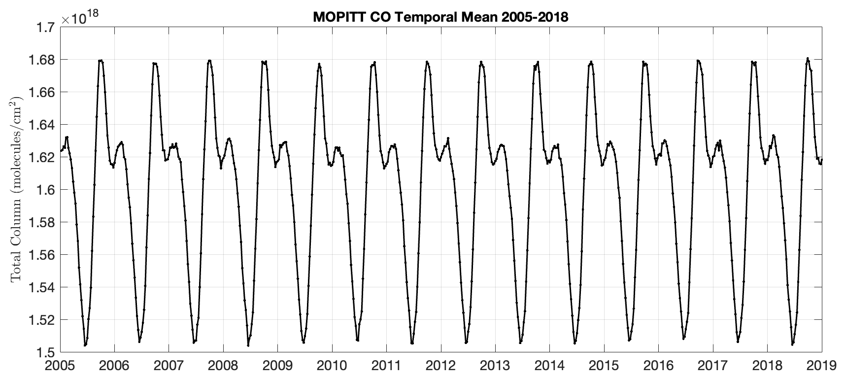
Figure 1 Spatially averaged time series of de-trended MOPITT CO over the period of 2005–2018 across the globe from 60° S to 60° N (in molec. cm⁻²).

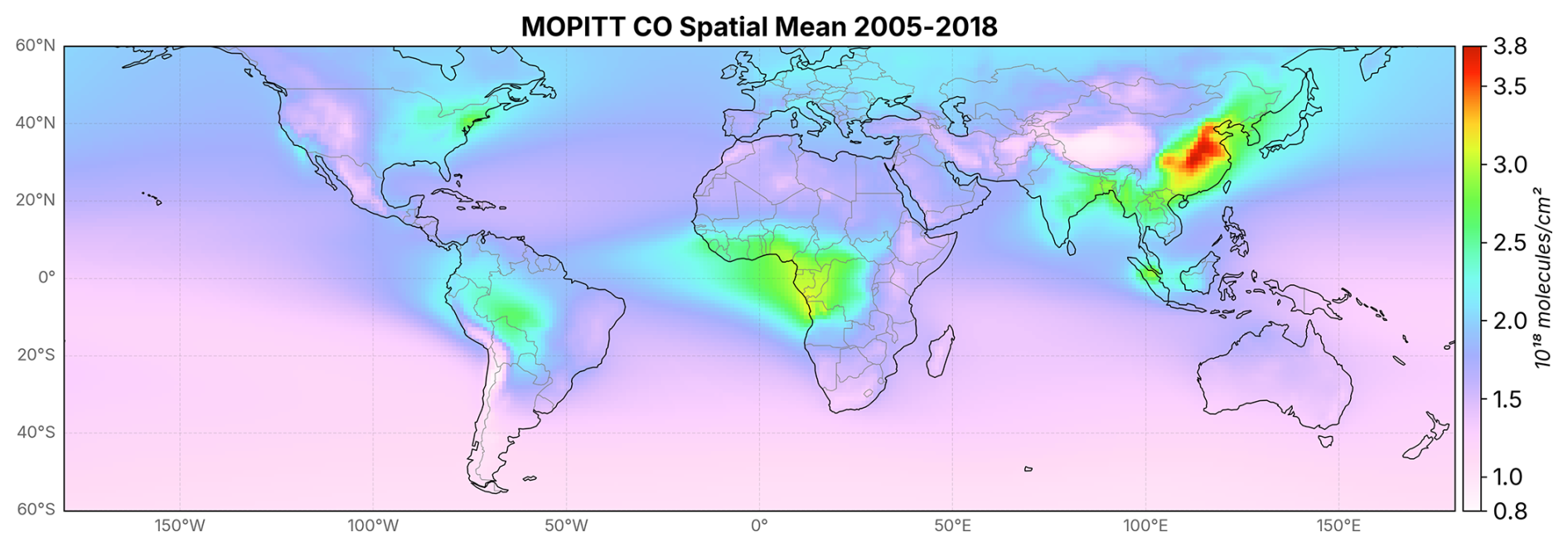
Figure 2 Temporally averaged global map of de-trended MOPITT CO over the period of 2005–2018 across the globe from 60° S to 60° N (in molec. cm⁻²).

3.2 Domain Independence and Separation of Modes for MOPITT CO

As discussed in Sect. 2.3.2, one of the first potential issues that needs to be addressed to produce physical EOF modes is whether or not the modes capture the local structure and if they are reproducible across differing subdomains. Before generating EOF modes, our data matrix of size (longitude, latitude, time) is reshaped into size (time, grid), and every grid point is mean-centered across time and then standardized. In Fig. 3, we show the first leading EOF mode for the dataset across the entire globe (a) and then recompute the first mode after subdividing the domain into North American (b), African (c), and Asian (d). To verify that these spatial patterns did not change over time, we recomputed the EOFs after segmenting the time series by year and determined that the patterns remained unchanged (they only showed negligible differences in magnitude). The spatial structure of the original pattern has been preserved in each of the three subdomains, showing us that the local and global structure for the pattern is the same, and therefore our dataset is independent of its domain.

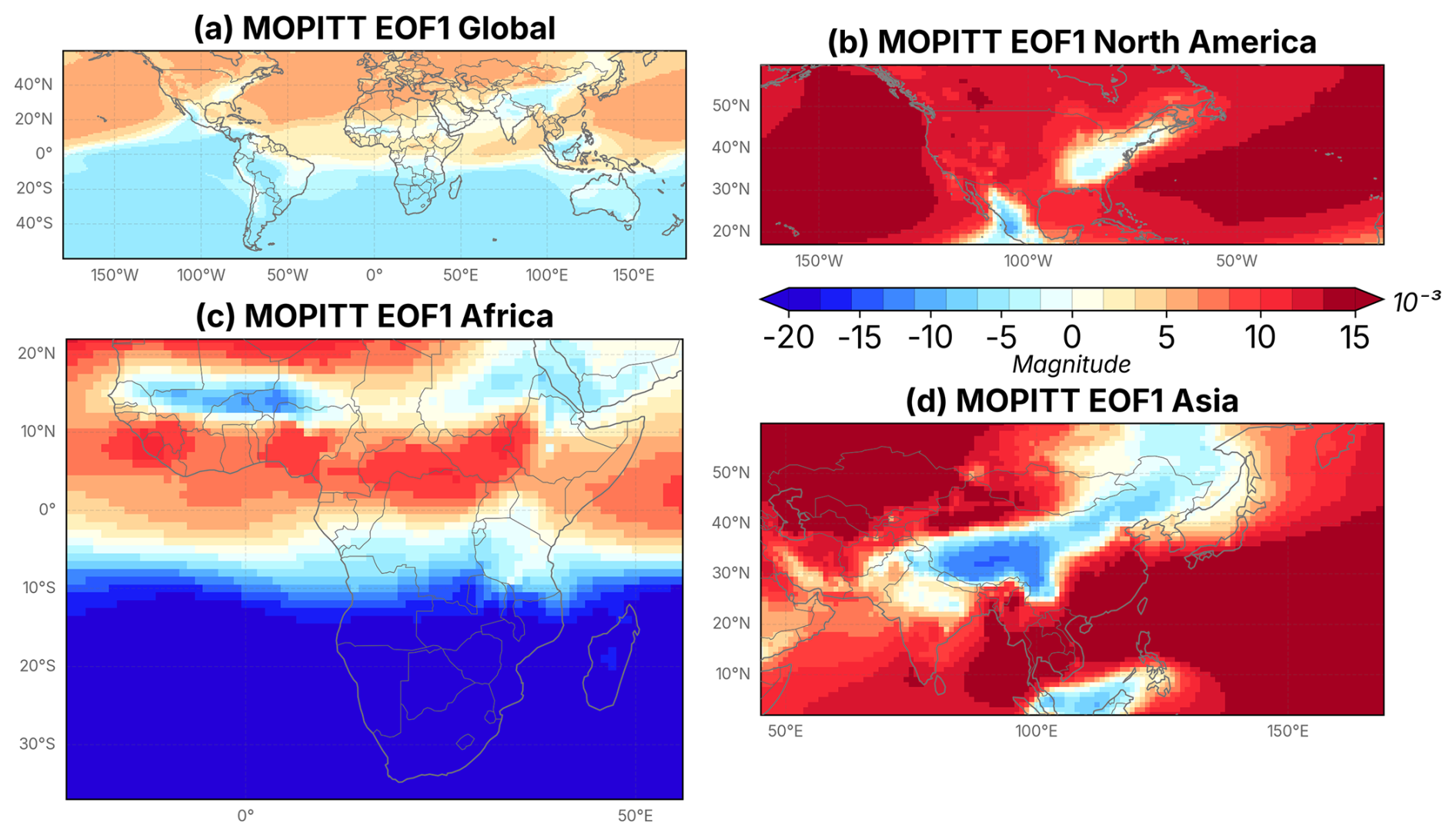
Figure 3 Spatial map showing the first EOF mode of MOPITT CO for (a) the globe, (b) North America, (c) Africa, and (d) Asia. All magnitudes are unitless, and all modes represented have unit norm.

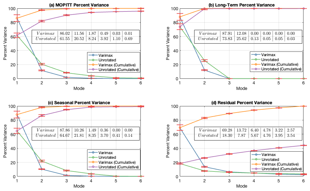
Figure 4 The percent variance that is explained by the first six normalized EOF modes for (a) the MOPITT dataset and (b) long-term, (c) seasonal, and (d) residual components after using an SSA decomposition. Results are shown globally for both varimax EOFs (blue) and unrotated EOFs (green). Additionally, we display the cumulative percent variance explained for varimax EOFs (orange) and unrotated EOFs (purple). Our error bars, computed using the North test, are shown in red.

In some problems, it is often a good idea to attempt varimax rotation to ensure that the resulting patterns are simple and easy to interpret (Kaiser, 1958; Horel, 1981; Richman, 1986), but in our case, there is not a real need to do so because our problem does not suffer from domain instability (Buell, 1975; Richman, 1986). To demonstrate that varimax does not improve our resulting modes, we show the eigenvalue spectrum of the first six unrotated EOF modes together with the spectrum of our varimax modes in Fig. 4. Each mode is plotted as a fraction of the percent variance, with the exact value shown within the text box in the middle of the plot. The varimax and unrotated modes are shown in blue and green, respectively, and the cumulative percent variance is shown in orange and purple. We compute the error bars using Eq. (9) for Δλ_k in Sect. 2.2.2 and plot the results in red. For our unrotated modes of the original MOPITT dataset in (a), the variance together with error bars (the length above/below each data value) are given by: 61.55±3.43 %, 20.52±1.143 %, 8.24±0.459 %, 3.92±0.218 %, 1.10±0.061 % and 0.69±0.038 %. After using varimax rotation, the percent variance of each mode was: 86.02±4.793 %, 11.56±0.644 %, 1.87±0.104 %, 0.49±0.027 %, 0.03±0.002 % and 0.01±0.001 %.

While our plots of percent variance for the varimax modes show better representation for mode 1 of every dataset compared to our unrotated modes, all of the remaining modes showed significantly worse representation (except the residual modes). None of these eigenvalues represent degenerate modes because their error bars do not overlap with adjacent neighbors. We note, however, that varimax modes 4, 5, and 6 have such a small percent variance that it is unlikely for them to rise above the level of noise and represent independent and important features. On the other hand, the higher modes of our unrotated EOFs have a much larger percent variance and are more likely to represent independent features, with modes 5 and 6 most likely representing noise. Comparing the cumulative percent variance for the first 3 MOPITT modes, we see our unrotated modes accounted for 90.3 % of the variance compared to 99.4 % for varimax. Because our third varimax mode only accounted for 1.87 % variance as opposed to 8.24 % for our unrotated mode, we could not guarantee that it would be well represented. We therefore decide to only analyze spatial patterns of the first 3 unrotated modes in our SSA decomposition, which comes at the cost of explaining 9.1 % less variance overall. We discuss the long-term, seasonal, and residual modes in greater detail in Sect. 3.3.

Finally, we note that our choice to display the first six modes does not represent an “optimal” representation of modes as could be determined using statistical tests for eigenvalues (Tipping and Bishop, 2002; Hendrikse et al., 2009; Isokääntä et al., 2020). This choice is made to ensure we display at least one potentially degenerate mode for both our varimax and unrotated EOFs. We also do this to show there is little motivation to keep more than 5 EOFs in our analysis, since each mode beyond the fifth adds a negligible (<1 %) amount of variance, except the residual modes.

3.3 Seasonal Decomposition for MOPITT CO

To visualize our SSA decomposition, rather than choosing a single grid point as an example, we plot a decomposition for the temporal mean of the dataset in Fig. 5 to show the average overall effect. Our results are plotted only for 2005–2009, as five yearly cycles were sufficient to show the effect of the decomposition. We show the decomposition for 4 different regions: Global (60° S–60° N), Northern Extratropics (25–60° N), Southern Extratropics (25–60° S), and Tropics (24° S–24° N).

The result is that the long-term component (red) has a yearly periodicity that reproduces the peaks of the original MOPITT series (blue), while the seasonal component (green) has a shorter temporal periodicity (6 months). The residual component (orange) shows the shortest periodicity, being on the order of 3 months. Note that in each case, the decomposition is phase shifted with reduced magnitude in comparison to MOPITT. When we compare the decomposition in each region, we see that the long-term component does the best job of reconstructing the original time series over the northern extratropics, as shown in Fig. 5b. The magnitude of the long-term component matches well with the original series, but peaks earlier in time. The same thing can be said regarding the southern extratropics, but with reduced magnitude relative to the original series. In Fig. 5d, we note that the long-term mode in the tropics is significantly shifted forward in time compared to the original series. Finally, we observe that the seasonal mode contributes the most to the reconstruction in the tropics since its magnitude relative to the original time series is largest.

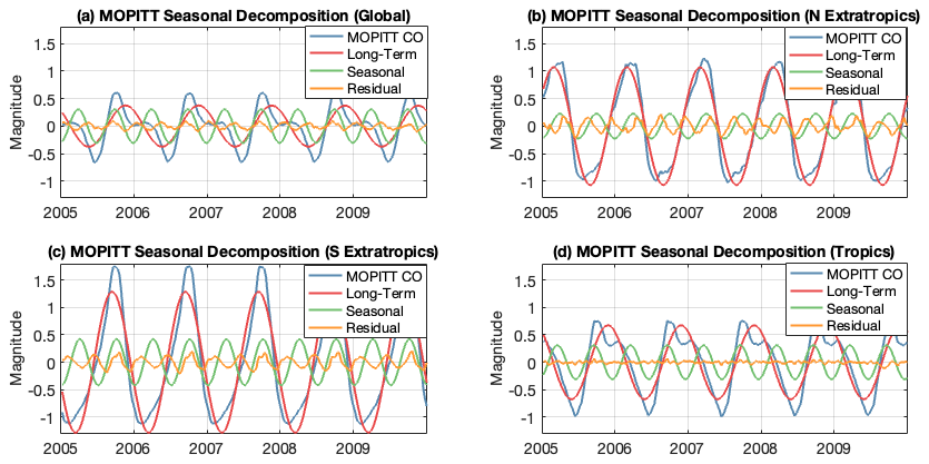
Figure 5 A time series plot of the rescaled MOPITT CO mean (blue) and the long-term (red), seasonal (green) and remainder (orange) components of the SSA decomposition shown from 2005–2009. We show the overall effect of the decomposition in 4 different regions: (a) Global (60° S–60° N), (b) Northern Extratropics (25–60° N), (c) Southern Extratropics (25–60° S), and (d) Tropics (24° S–24° N).

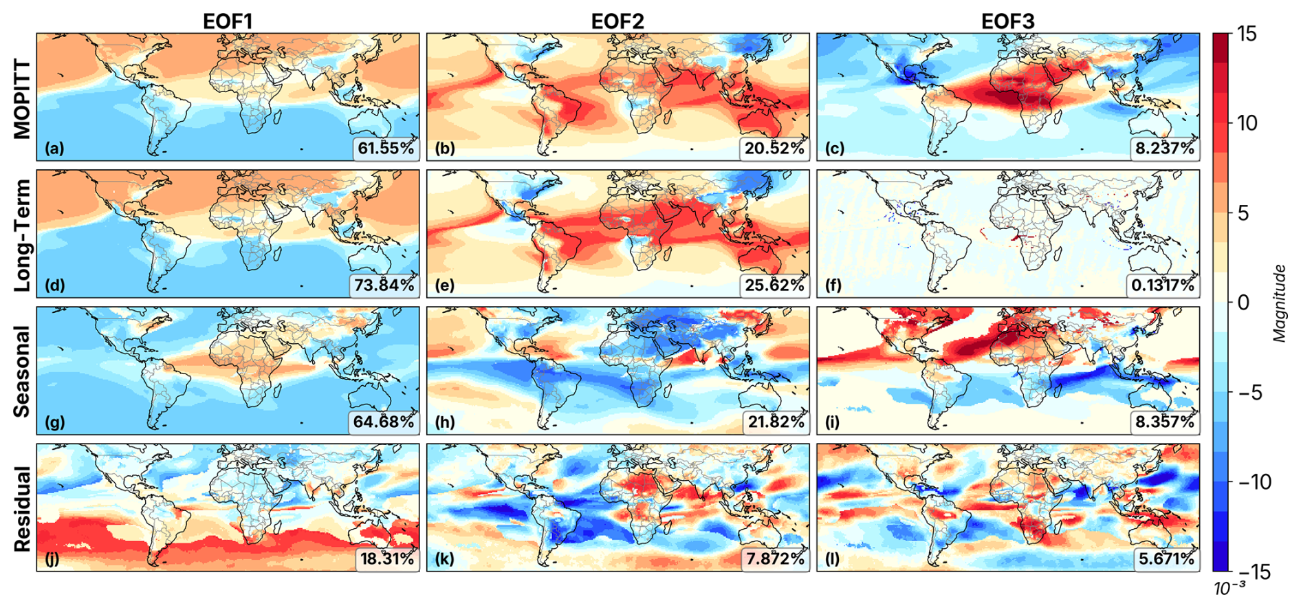
Figure 6 Spatial maps of the first 3 unrotated EOF modes of the (a–c) MOPITT dataset and its (d–f) long-term, (g–i) seasonal, and (j–l) residual components after using a SSA decomposition. The percent variance that is explained for each mode is displayed at the bottom right corner. All magnitudes are unitless, and all modes represented have unit norm.

By implementing SSA on each grid point, we produce 3 matrices, each with the same size as our original dataset, which are again mean-centered and standardized. We then conduct EOF analysis on the resulting matrices, displaying the first 3 global modes for MOPITT in Fig. 6 together with the first 3 modes of the long-term, seasonal, and remainder datasets. While there are some differences in magnitude and percent variance, we note that the first two long-term EOF modes reproduce the spatial pattern of the first two modes for the original MOPITT CO patterns. Examination of the third long-term EOF mode shows that the pattern appears to be noise, as indicated by the low percent variance and the complete lack of any spatial structure. We also note that there is a very similar structure between the third MOPITT EOF mode and the first Seasonal EOF mode; however, the first seasonal mode has a larger contrast between the positive and negative patterns, which is especially noticeable in Northeastern Asia and the east coast of the United States. The structure for seasonal modes 2 and 3, as well as all three residual modes, represents patterns distinct from our MOPITT EOF modes before we performed SSA on the data.

We also note that according to Fig. 6d, our long-term EOF mode 1 has the largest positive and negative anomalies in the extratropics. This observation is consistent with our time series in Fig. 5b and c, which showed that the long-term mode did the best job of matching the magnitude and phase of the original MOPITT time series in this region. Similarly, our seasonal EOF mode 1 in Fig. 6g showed the largest anomaly in the tropics. This is consistent with the time series of our seasonal mode in Fig. 5d, which had the largest magnitude relative to the original time series. A reduced influence of the long-term mode and a corresponding increase in the influence of the seasonal mode in the tropics is consistent with CO having a shorter lifetime in this region.

Our intention in performing EOF analysis was that each EOF mode would represent the variability from either a source or sink in CO; however, the patterns depicted in Fig. 6 do not correlate with physically separable sources. If each mode represented a source of CO, then we would expect to see modes that correlated with variability due to fossil fuel burning, biomass burning, biogenic oxidation, or CH₄ oxidation. However, none of the modes depicted in Fig. 6 show patterns of variability that can be directly connected with source distributions, nor do they appear to directly correspond with synoptic weather patterns or transport pathways.

As an example, let us attempt to connect MOPITT EOF 2 with fossil fuel burning. If we attempt the interpretation that blue areas represent areas with high contributions of fuel burning, this would be inconsistent with our knowledge of fossil fuel burning as a source of CO. While we do see significant areas of blue highlighted on the east coast of the United States which is consistent with combustion, the pattern shows too little activity over Eastern China and India and higher activity over Russia than expected. Similarly, when we examine EOF 3, we see a pattern that has some consistency with biomass burning in Africa and South America; however, the features are far too smeared to be a potential interpretation. For example, the pattern stretches too far across oceanic regions as well as the Sahara and Saudi Arabia to be classified as potential fire activity. For similar reasoning, it would not make sense for us to interpret this as a pattern of biogenic emission.

When examining EOF mode 1, we see a very clear boundary between the NH and SH as indicative of the annual cycle in CO caused by the combination of larger combustion activity and lower hydroxide radicals in the NH during the winter season. This interpretation is consistent with an observation we state in Sect. 3.3 on spectral analysis and time scales, which is that the time scale for EOF 1 is dominated by annual/semiannual variation.

The majority of the areas with the highest contrast in Residual EOF mode 1 are seen to be over oceanic regions, which suggests the possibility of a connection between Residual mode 1 and oceanic variability. However, these patterns do not match the variation of CO due to oceanic cycles, such as patterns as shown in Conte et al. (2019). This could be because we would expect oceanic variability to be strongest near the surface, and patterns due to surface variations would be obscured by the changes in CO throughout other areas of the atmosphere, which we are accounting for by using total column data. This could also be because budgets for oceanic cycles of CO vary widely both spatially and temporally due to changing environmental conditions (Ji et al., 2025).

Examining the remaining seasonal and residual patterns, we see patterns that could be indicative of regional-scale transport; however, verification and further discussion of these modes is beyond the scope of our analysis at this time.

3.4 Spectral Analysis and Time Scales

In Fig. 7, we display the principal component time series for the original MOPITT dataset as well as the long-term, seasonal, and residual components. We first note that the first two long-term principal components have very similar periodic patterns as the original 2 MOPITT modes, while the third mode is, of course, noise because, as we have already seen, the third long-term EOF pattern had no spatial structure. We also see that the first two seasonal components have a similar periodic pattern to the third MOPITT component, even though we saw from Fig. 6 that the second seasonal EOF has a very different spatial structure. The long-term modes have the largest period, while the seasonal components have shorter periodicity, and the residual modes have the shortest.

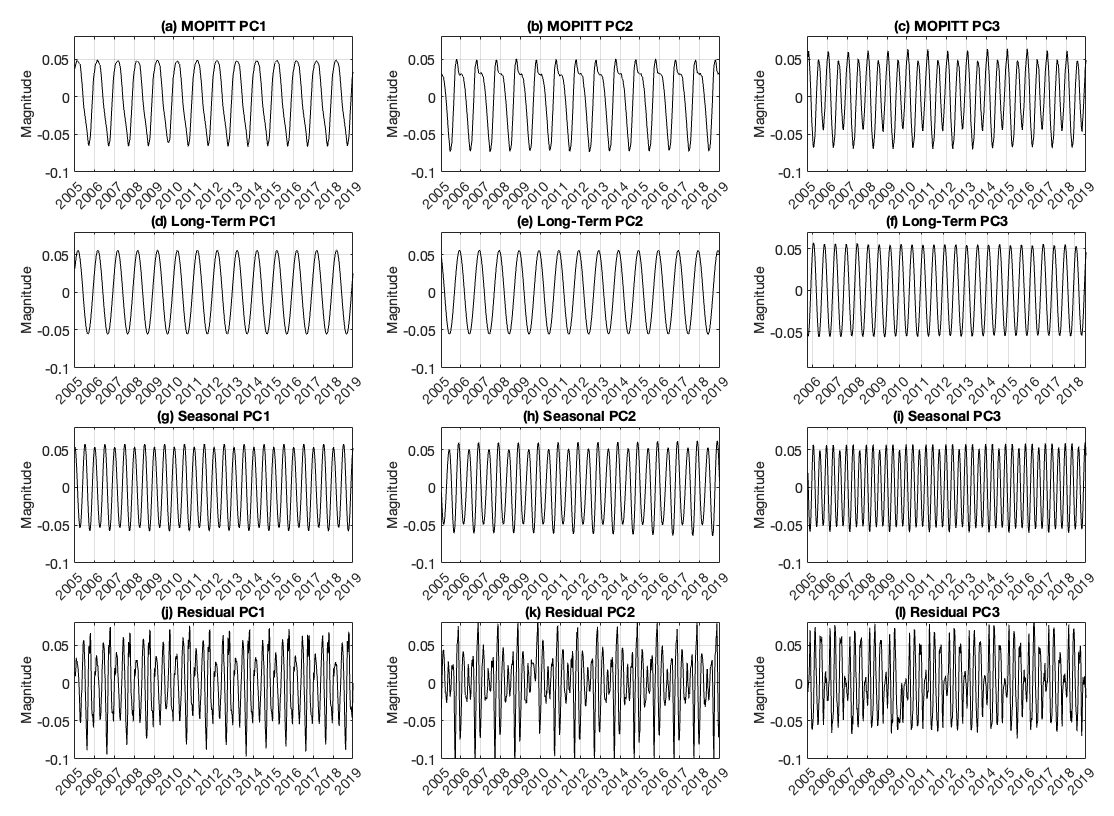
Figure 7 Time series for the first 3 principal components of the (a–c) MOPITT dataset and its (d–f) long-term, (g–i) seasonal, and (j–l) residual components after using an SSA decomposition. All magnitudes are unitless, and all modes represented have unit norm.

To determine the most dominant time scale for a given mode, we used Fourier transforms to compute the power spectral density of each principal component and then used a numerical trapezoid rule to determine the total cumulative power as a percentage, which is then plotted in Fig. 8 on a logarithmic scale. The percent of total power is labeled for a period of oscillation for 100 d, 1 year, and 1000 d. We note that in this context, having time scales longer than the lifetime of CO still makes physical sense because some variability of CO is driven by large-scale weather patterns. The intrahemispheric mixing time is about 6 months, while interhemispheric mass exchanges can happen across 1–2 years (Bowman and Cohen, 1997). Variability on this time scale could also be indicative of changes to climate drivers. For example, deforestation over several years may lead to long-term reduction of biogenic and fire emissions, while urbanization may lead to an increase in anthropogenic emissions. A dotted line and the value t_max indicate the period of oscillation that contributed the largest amount to the total power. For example, examining MOPITT Spectrum Mode 1, we see that 1.3 % of power is from periods of 100 d or smaller, 26.9 % of power is from periods of 1 year or smaller, and 43.2 % of power is from periods of 1000 d or smaller. We see that the first two MOPITT patterns correspond to variation dominated by an annual/semi-annual cycle, while the third mode is dominated by seasonal changes on the order of 3 months. Our long-term EOFs reproduce our original 2 modes, while our seasonal EOFs show dominant time scales on the order of 3 or 2 months, and our residual modes show dominant time scales on the order of 2 months or less.

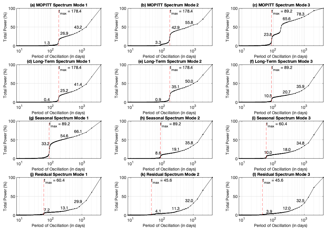
Figure 8 The cumulative percent total power for each principal component. Power values are labeled at 100 d, 1 year, and 1000 d. The dotted line and the value t_max indicate the period of oscillation that has contributed the largest amount to the total power.

3.5 Time Dependence and Non-Stationarity of Modes

As discussed in Sect. 2.2.3, one weakness of EOF analysis is that even though the principal component time series are constructed to be uncorrelated, it is not necessarily appropriate to assume that they represent independent processes, which complicates the interpretation of assigning physical meaning to the modes. Only in the special case that the data is Gaussian does it follow that uncorrelated random variables are then deemed independent. In Fig. 9, we plot the mean skewness field for MOPITT CO over the period of interest from 2005–2018. It is standard to consider values of absolute skewness less than 0.5 to have negligible skewness corresponding to a relatively symmetric distribution, while values between 0.5 and 1.0 are moderately skewed, and values larger than 1.0 are highly skewed. Contour lines are shown for skewness values of −1, −0.5, +0.5, and +1.0 to highlight areas that have a notable degree of skewness.

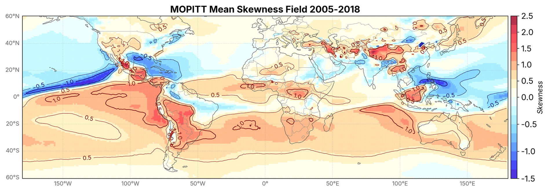
Figure 9 A spatial plot showing the mean skewness field of MOPITT CO from 2005–2018. Contour lines are shown to highlight skewness values of −1.0, −0.5, 0.5, and 1.0, indicating regions that are moderately or heavily skewed.

We note that these sharp gradients in skewness in Fig. 9 are driven by long-term seasonal changes in sources and sinks depending on the region. Regions of low skewness generally indicate places where pollution levels are relatively constant throughout the year, with few extreme highs or lows. High positive skewness values indicate a larger number of extreme pollution events are occurring in the area, and may be interpreted as local enhancement from long-term transport. For example, we interpret the high skewness we see in central Africa as transport due to biomass burning plumes which frequently move westward (Krishnamurti et al., 1996; Fisher et al., 2015). Similarly, large skewness across South America may be indicative of the secondary contribution of isoprene oxidation near the equator. This observation is consistent with Fisher et al. (2015), who discuss how isoprene in South America is uplifted to sufficient levels to easily react with OH, where it is slowly transported far south and into the extratropics. The bands with high skewness across the SH are consistent with the north/south movement of the inter-tropical convergence zone due to exchange of CO through the Hadley circulation (Bowman and Cohen, 1997; Bowman, 2006). The skewness patterns we see in the NH are more diverse and are indicative of the seasonal changes in fossil fuel usage, which vary by region and sector.

Overall, we see from Fig. 9 that our dataset has significant skewness in the SH, especially in South America, as well as over China, Indonesia, and East Asia. This indicates that we cannot consider our dataset to be approximately Gaussian, and this is a potential explanation for why our principal components show significant dependence in the distributions of their spectral responses. EOF analysis assumes that the dataset is stationary so that the mean and temporal covariance remain constant in time, which is done to ensure that the first and second moments (the mean and covariance) of random variables can be determined using a limit of simple summations (or integrals). In practice, this assumption is rarely realistic with physical data. An equivalent statement is that the temporal autocorrelation is constant as a function of lag time τ. If we consider the mean and covariance of CO, it would be realistic to assume that these statistics should be a function of time because their sources and sinks are correlated temporally. If we imagine a smokestack emitting CO at a fixed location, the CO measured in the future is highly correlated with the amount of CO in the present. This brings us to our next main point, which is that another reason why our modes cannot be interpreted in terms of individual sources and sinks lies in the non-stationarity of the MOPITT dataset, which remains unaccounted for in standard EOF analysis and is a fact we will now show.

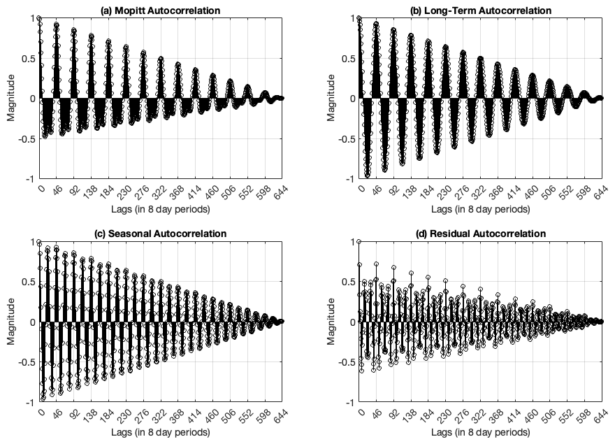
Figure 10 The autocorrelation for (a) MOPITT CO as well as the autocorrelation of the (b) long-term, (c) seasonal, and (d) residual modes after using an SSA decomposition, plotted as a function of lag time (measured in 8 d periods).

As shown in Fig. 10, the autocorrelation for the original MOPITT time series, as well as each component from the seasonal decomposition, does not decay to zero but instead shows periodic variation that persists across time. The MOPITT series has a positive correlation that peaks for every year exactly and shows two negative peaks, both of which also recur at intervals of 1 year. We could therefore consider the MOPITT autocorrelation as being a sum of three periodic components. The long-term and seasonal autocorrelation are simpler functions, and both have a single periodic component that peaks exactly once per year and 6 months, respectively. The residual autocorrelation, like MOPITT, is a sum of periodic processes. It is important to note that we cannot force the dataset to become stationary by removing an annual cycle, because the autocorrelation represents a superposition of multiple periodic processes. We may therefore consider both the long-term and seasonal series to be wide-sense cyclostationary processes since they have a periodic temporal mean and a periodic temporal autocorrelation. Because the MOPITT series and residual series are composed of multiple periodic processes, we may consider them to be wide-sense polycyclostationary. We conclude this discussion by mentioning that in future studies, it may be worth exploring the use of cyclostationary EOF (CSEOF) analysis on either the original time series or on the seasonal modes. CSEOF analysis is a method that is well-suited for datasets that possess autocorrelation functions of this type (Kim et al., 2015). Unlike traditional EOF methods that assume stationary covariance, CSEOF can better capture evolving physical modes, a feature essential for analyzing atmospheric time series.

4 Conclusions

In this study, we explored the application of EOF analysis to evaluate whether CO source signatures can be discerned from observed CO abundances. We hypothesized that spatial and temporal differences in CO are influenced by surface emission patterns, including contributions from CH₄ and NMHCs, atmospheric transport, and reactions with OH. Rather than interpreting physical patterns, we emphasized the methodological rationale and limitations underlying our findings.

Our results in Fig. 3 demonstrate that EOF modes derived from MOPITT CO columns are not domain-dependent, as generating regional domains yielded spatial patterns nearly identical to those from a global domain. Using the North test, we showed in Fig. 4 that unrotated EOF modes provided better data representation than varimax modes. Consequently, seasonal analysis via SSA was performed exclusively on unrotated modes due to their improved representation and domain-independence, which are characteristics specific to our dataset. However, we emphasize that this decision should not be generalized across all climate datasets.

Plots of cumulative percent total power for the principal components in Fig. 8 revealed that lower-order modes capture long-term variability, while higher-order modes reflect shorter-term fluctuations. Each mode exhibited power distributed across a range of frequencies, suggesting that variability arises from a combination of time scales rather than isolated periodicities.

Seasonal skewness analysis from Fig. 9 confirmed that, although the principal component time series are uncorrelated, they are not independent due to the non-Gaussian nature of the dataset. As a result, they cannot be directly associated with distinct sources or sinks. We also discussed how these sharp gradients in skewness are driven by long-term seasonal changes of CO.

The first unrotated EOF in Fig. 6a and the long-term pattern in Fig. 6d reflect the annual/semiannual cycle of CO. However, the temporal dependence among modes, non-stationarity of the time series, and our use of total column data may confound distinct variability patterns, making it difficult to attribute higher-order modes to specific sources or sinks. Future work should investigate CO statistics across vertical levels to determine whether time-independent modes can be identified and whether Gaussian assumptions are better satisfied.

As demonstrated in the autocorrelation plots (Fig. 10), the MOPITT CO time series exhibits wide-sense polycyclostationarity. Because CSEOF analysis is designed to handle time-evolving covariance structures of this type, we believe it is worthwhile to consider its utility to study patterns in MOPITT CO and other atmospheric data in the future. If CSEOF can successfully separate source-specific variability, methods such as Covariance Discrimination Analysis (CDA) can be utilized, which compare datasets based on covariance structures. This may enable the identification of statistical discrepancies between modeled and observed CO, and help attribute these to biases in source attribution, including fossil fuel combustion, biomass burning, and oxidation of CH₄ and hydrocarbons.

Finally, we acknowledge that these limitations stem from the highly diffusive nature of atmospheric transport, the reactive chemistry of CO and OH, and the limited resolution of column-averaged CO observations. These factors obscure the distinction between regional sources and broader background CO. We propose that a multi-species, multi-scale approach, leveraging synergies among diverse data sources and incorporating advanced methods – such as pattern recognition, dimensionality reduction, and machine learning – offers a promising path forward in attributing source signatures to physical processes. This is particularly relevant given the recent availability of high-resolution atmospheric composition datasets.

Appendix A

A1 Eigenvectors of Temporal and Spatial Covariance Matrices

Suppose F is an n×m matrix where measurements are taken over n points in time and over a spatial grid with m points. We define the m×m spatial covariance matrix as R=F^TF and the n×n temporal covariance matrix as L=FF^T. Note that here we do not normalize our covariance matrices using the sample size purely to make the rest of this discussion (and the subsequent discussion in Appendix A2) easier to follow. In the case that the number of gridpoints is very large and m≫n, it becomes computationally infeasible to perform an eigendecomposition on R. It is instead desirable to decompose the much smaller covariance matrix L and project the resulting PC time series to compute the EOF spatial patterns, which are eigenvectors of R. We begin by performing an eigendecomposition on the spatial covariance matrix R to yield the eigenvector matrix C, which corresponds to the EOF spatial patterns and satisfies:

$$\begin{array}{}\text{(A1)}& \mathbf{RC}=\mathbf{C}\mathbf{\Lambda }\end{array}$$

Multiplying on the LHS yields:

$$\begin{array}{}\text{(A2)}& \mathbf{FRC}={\mathbf{FF}}^T\mathbf{FC}=\mathbf{LFC}\end{array}$$

and multiplication by F on the RHS then gives us:

$$\begin{array}{}\text{(A3)}& \mathbf{L}\left(\mathbf{FC}\right)=\left(\mathbf{FC}\right)\mathbf{\Lambda }\end{array}$$

And defining A=FC we have:

$$\begin{array}{}\text{(A4)}& \mathbf{LA}=\mathbf{A}\mathbf{\Lambda }\end{array}$$

which shows that A is the matrix of eigenvectors for L, while the eigenvalues Λ are the same as for R. We note that while the eigenvectors C of R are size m×m and represent a spatial pattern, the eigenvector matrix A of L is size n×n and represents the principal component (PC) time series constructed by projecting the original matrix F onto the EOF patterns C. We can reconstruct the original matrix F using the EOF spatial patterns and the un-normalized PC time series as:

$$\begin{array}{}\text{(A5)}& \mathbf{F}={\mathbf{AC}}^T\end{array}$$

The fact that A is not normalized is apparent from the PCA property of R:

$$\begin{array}{}\text{(A6)}& \begin{array}{rl}{\mathbf{A}}^T\mathbf{A}& ={\left(\mathbf{FC}\right)}^T\mathbf{FC}={\mathbf{C}}^T{\mathbf{F}}^T\mathbf{FC}={\mathbf{C}}^T\mathbf{RC}\\ & ={\mathbf{C}}^T\mathbf{C}\mathbf{\Lambda }{\mathbf{CC}}^T=\mathbf{\Lambda }\end{array}\end{array}$$

which shows us that $\left|\right|{\mathbf{A}}^T\mathbf{A}\left|\right|=\left|\right|\mathbf{\Lambda }\left|\right|\ne \mathbf{I}$. We can therefore define a normalized PC time series Φ by dividing each term by ${\mathit{\lambda }}^{\mathrm{1}/\mathrm{2}}$:

$$\begin{array}{}\text{(A7)}& \mathbf{\Phi }=\mathbf{FC}{\mathbf{\Lambda }}^{-\mathrm{1}/\mathrm{2}}=\mathbf{A}{\mathbf{\Lambda }}^{-\mathrm{1}/\mathrm{2}}\end{array}$$

then it follows that Φ is orthogonal:

$$\begin{array}{}\text{(A8)}& {\mathbf{\Phi }}^T\mathbf{\Phi }={\left(\mathbf{A}{\mathbf{\Lambda }}^{-\mathrm{1}/\mathrm{2}}\right)}^T\mathbf{A}{\mathbf{\Lambda }}^{-\mathrm{1}/\mathrm{2}}=\left({\mathbf{A}}^T\mathbf{A}\right){\mathbf{\Lambda }}^{-\mathrm{1}}=\mathbf{\Lambda }{\mathbf{\Lambda }}^{-\mathrm{1}}=\mathbf{I}\end{array}$$

This expression of Φ is important, because it allows us to express the singular value decomposition of the matrix F as:

$$\begin{array}{}\text{(A9)}& \mathbf{F}=\mathbf{\Phi }{\mathbf{\Lambda }}^{\mathrm{1}/\mathrm{2}}{\mathbf{C}}^T=\mathbf{\Phi }\mathbf{\Sigma }{\mathbf{C}}^T\end{array}$$

If we use the singular value decomposition for F in the covariance matrices, then we recover the eigendecompositions for both R and L:

$$\begin{array}{}\text{(A10)}& {\displaystyle }\mathbf{R}={\mathbf{F}}^T\mathbf{F}={\left(\mathbf{\Phi }\mathbf{\Sigma }{\mathbf{C}}^T\right)}^T\mathbf{\Phi }\mathbf{\Sigma }{\mathbf{C}}^T=\mathbf{C}\mathbf{\Lambda }{\mathbf{C}}^T\text{(A11)}& {\displaystyle }\mathbf{L}={\mathbf{FF}}^T={\left(\mathbf{\Phi }\mathbf{\Sigma }{\mathbf{C}}^T\right)}^T\mathbf{\Phi }\mathbf{\Sigma }{\mathbf{C}}^T=\mathbf{\Phi }\mathbf{\Lambda }{\mathbf{\Phi }}^T\end{array}$$

so we see that orthogonal eigenvector matrices for R and L are the normalized EOF spatial patterns C and the PC time series Φ, respectively. Therefore, when n≫m and we cannot easily compute C, our strategy is to perform eigendecomposition on L to find Φ, and then determine C by rearranging the SVD expression:

$$\begin{array}{}\text{(A12)}& \mathbf{C}=\left({\mathbf{F}}^T\mathbf{\Phi }\right){\mathbf{\Lambda }}^{-\mathrm{1}/\mathrm{2}}=\mathbf{G}{\mathbf{\Lambda }}^{-\mathrm{1}/\mathrm{2}}\end{array}$$

where G=F^TΦ. The original matrix F can then be reconstructed using the full rank expression for the SVD. If we are using correlation matrices so that F has zero mean and has been scaled by its standard deviation, the original matrix in physical space F^* is given by:

$$\begin{array}{}\text{(A13)}& {\mathbf{F}}^{*}=\mathbf{F}\mathrm{std}\left(\mathbf{F}\right)+\mathrm{mean}\left(\mathbf{F}\right)=\left(\mathbf{\Phi }\mathbf{\Sigma }{\mathbf{C}}^T\right)\mathrm{std}\left(\mathbf{F}\right)+\mathrm{mean}\left(\mathbf{F}\right).\end{array}$$

A2 Equivalence of Determining EOFs and PCs Using Eigenvector Decomposition and SVD

In the case of eigenvector decomposition, we describe three cases in accordance with the size of F as shown in Table A1. When we have m≫n, so the spatial grid is large, then L=FF^T has size n×n, and as described before, we compute the eigendecomposition of L to determine the PC time series, which are the column vectors of Φ. In MATLAB, we would simply use $\left[\mathbf{\Phi },\mathbf{\Lambda }\right]=\mathrm{eig}\left(\mathbf{L}\right)$ to compute the normalized eigenvectors and the eigenvalues. We can then compute the matrix G and find the EOF spatial patterns, which are the column vectors of C (or the row vectors of C^T).

In the case that n≫m so the time points are large, then R=F^TF has size m×m and we first compute the EOF spatial patterns C which are the normalized eigenvectors of R, and are found in Matlab as $\left[\mathbf{C},\mathbf{\Lambda }\right]=\mathrm{eig}\left(\mathbf{R}\right)$. We then determine the PC time series by projecting the original matrix using Φ=FC.

When m≈n, then either method from above would be appropriate to compute the EOFs and PCs. It would also be appropriate (and equivalent) to compute the singular value decomposition of F using Eq. (5) which is determined in matlab as $\left[\mathbf{\Phi },\mathbf{\Sigma },\mathbf{C}\right]=\mathrm{svd}\left(\mathbf{F}\right)$, where the singular values Σ are the square roots of the eigenvalues Λ. In this case, the left singular vectors are the normalized PC time series, and the right singular vectors are the normalized EOF spatial patterns.

Table A1 Computation of EOFs and PCs shown in three cases depending on the size of F. When m≠n, it is appropriate to use eigenvector decomposition on whichever covariance matrix is smallest. When m≈n, eigenvector decomposition and SVD yield equivalent results.

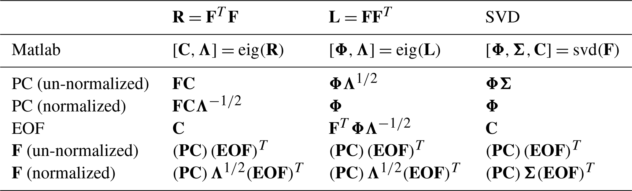
A3 Estimate of N^* in Terms of an AR1 Process

The following is a derivation of N^*, which we use for the estimate for the effective sample size as discussed in Hartmann (2016). Red noise is characterized by the property that future observations are predicted using a linear combination of the previous observations plus a random noise term. Red noise has exponential autocorrelation, which decays according to:

$$\begin{array}{}\text{(A14)}& r\left(\mathit{\tau }\right)=\exp \left(-\mathit{\tau }/T\right)\end{array}$$

where τ is the lag time and T is the e-folding time (the time interval over which the autocorrelation drops to $\mathrm{1}/e$). For a first-order process, note that if we define the autocorrelation at one time step Δt to be:

$$\begin{array}{}\text{(A15)}& a=r\left(\mathrm{\Delta }t\right)=\exp \left(-\mathrm{\Delta }t/T\right)\end{array}$$

then the autocorrelation evaluated n time steps in the future can be written as:

$$\begin{array}{}\text{(A16)}& r_n=r\left(n\mathrm{\Delta }t\right)=\left(\exp \right(-\mathrm{\Delta }t/T){)}^n=a^n.\end{array}$$

We can express N^* in terms of the true sample size N as follows (Thiébaux and Zwiers, 1984):

$$\begin{array}{}\text{(A17)}& N^{*}={\displaystyle \frac{N}{\sum _{n=-N-\mathrm{1}}^{N+\mathrm{1}}\left(\mathrm{1}-{\displaystyle \frac{\left|n\right|}{N}}\right)r_n}}.\end{array}$$

If we further assume that N is very large and that our process is AR1, Eq. (A17) can be written as:

$$\begin{array}{}\text{(A18)}& N^{*}={\displaystyle \frac{N}{\sum _{n=-\mathrm{\infty }}^{\mathrm{\infty }}{r}_n}}={\displaystyle \frac{N}{\mathrm{1}+\mathrm{2}\left(\sum _{n=\mathrm{1}}^{\mathrm{\infty }}{a}^n\right)}}\end{array}$$

and we see the sum in the denominator of Eq. (A18) is a geometric series with $\left|a\right|<\mathrm{1}$ which converges to the value:

$$\begin{array}{}\text{(A19)}& \sum _{n=\mathrm{1}}^{\mathrm{\infty }}{a}^n=a+a^{\mathrm{2}}+\mathrm{\dots }+={\displaystyle \frac{a}{\mathrm{1}-a}}.\end{array}$$

Substituting Eq. (A19) into Eq. (A18) then yields our estimate for N^* given by Eq. (8) in our methods section. We reiterate that this estimation is only valid for a large number of independent samples and when we assume our time series is an AR1 stochastic process. This is because we rely on the property given by Eq. (A16) of AR1 processes and large N to both be true to guarantee that Eq. (A18) is valid. We also rely on N to be large for the sum in Eq. (A19) to be accurate.

A4 Jointly Gaussian Distributions Are Independent

In this section, we verify the fact that jointly Gaussian distributions have modes that are uncorrelated and independent. To see this fact, we note that in the case of 2 random variables, if X₁ and X₂ are uncorrelated and jointly Gaussian, then the associated covariance matrix is diagonal and the joint PDF takes the form:

$$\begin{array}{}\text{(A20)}& \begin{array}{rl}{f}_X& (x_{\mathrm{1}},x_{\mathrm{2}})={\displaystyle \frac{\mathrm{1}}{\sqrt{(\mathrm{2}\mathit{\pi }{)}^{\mathrm{2}}{\mathit{\sigma }}_{\mathrm{1}}^{\mathrm{2}}{\mathit{\sigma }}_{\mathrm{2}}^{\mathrm{2}}}}}\exp \\ & \left(-{\displaystyle \frac{\mathrm{1}}{\mathrm{2}}}\left({\displaystyle \frac{(x_{\mathrm{1}}-{\mathit{\mu }}_{\mathrm{1}}{)}^{\mathrm{2}}}{{\mathit{\sigma }}_{\mathrm{1}}^{\mathrm{2}}}}+{\displaystyle \frac{(x_{\mathrm{2}}-{\mathit{\mu }}_{\mathrm{2}}{)}^{\mathrm{2}}}{{\mathit{\sigma }}_{\mathrm{2}}^{\mathrm{2}}}}\right)\right)\end{array}\end{array}$$

which can be written as:

$$\begin{array}{}\text{(A21)}& {\displaystyle }\begin{array}{rl}{f}_X(x_{\mathrm{1}},x_{\mathrm{2}})& ={\displaystyle \frac{\mathrm{1}}{\sqrt{\mathrm{2}\mathit{\pi }{\mathit{\sigma }}_{\mathrm{1}}^{\mathrm{2}}}}}\exp \left(-{\displaystyle \frac{\mathrm{1}}{\mathrm{2}}}\left({\displaystyle \frac{(x_{\mathrm{1}}-{\mathit{\mu }}_{\mathrm{1}}{)}^{\mathrm{2}}}{{\mathit{\sigma }}_{\mathrm{1}}^{\mathrm{2}}}}\right)\right)\\ & \times {\displaystyle \frac{\mathrm{1}}{\sqrt{\mathrm{2}\mathit{\pi }{\mathit{\sigma }}_{\mathrm{2}}^{\mathrm{2}}}}}\exp \left(-{\displaystyle \frac{\mathrm{1}}{\mathrm{2}}}\left({\displaystyle \frac{(x_{\mathrm{2}}-{\mathit{\mu }}_{\mathrm{2}}{)}^{\mathrm{2}}}{{\mathit{\sigma }}_{\mathrm{2}}^{\mathrm{2}}}}\right)\right)\end{array}\text{(A22)}& {\displaystyle }=f_X\left(x_{\mathrm{1}}\right)\times f_X\left(x_{\mathrm{2}}\right).\end{array}$$

It follows that X₁ and X₂ are independent.