On the capability of the Changing Atmosphere Infra-Red Tomography explorer (CAIRT) candidate mission to constrain O₃ and H₂O in the upper troposphere and lower stratosphere

The Changing Atmosphere Infra-Red Tomography Explorer (CAIRT) is a satellite mission concept that was proposed within ESA's Earth Explorer 11 (EE11) programme. Although it was not selected for implementation in the EE11 competition, the CAIRT concept was assessed as scientifically and technically mature and could be implemented under another ESA framework or through international collaboration. The mission is conceived to achieve a step change in our understanding of the coupling between atmospheric circulation, composition, and regional climate. The CAIRT concept is based on limb infrared tomography of the atmosphere from the troposphere to the lower thermosphere (between ∼ 5 and ∼ 115 km altitude) with a ∼ 400 km-wide swath, providing a three-dimensional view of atmospheric structure at unprecedented scales.

This paper investigates the capability of CAIRT to resolve gradients of ozone (O₃) and water vapour (H₂O) in the upper troposphere and lower stratosphere (UTLS) using an Observing System Simulation Experiment (OSSE). In this experiment, a reference atmosphere – the nature run in OSSE terminology – is built from the Copernicus Atmosphere Monitoring Service (CAMS) control simulation between October 2021 and March 2022. The nature run is used to synthesise CAIRT observations of O₃ and H₂O, employing a CAIRT orbit simulator and a simulator that accounts for CAIRT's expected measurement errors, vertical and along-track vertical resolution. Simulated CAIRT observations are then assimilated with the Belgian Assimilation System for Chemical ObsErvations (BASCOE) to produce analyses of O₃ and H₂O (the assimilation run). To quantify the added value of CAIRT data, a BASCOE control run without CAIRT assimilation is also performed. For comparison, simulated Aura Microwave Limb Sounder (MLS) O₃ and H₂O observations are also assimilated, allowing the performance of CAIRT to be evaluated relative to this reference instrument.

The results show that (1) CAIRT O₃ observations are able to constrain BASCOE analyses down to 7 km altitude – several kilometres lower (and thus better) than MLS; and (2) H₂O observations can constrain BASCOE down to the tropopause region, with slightly better performance than MLS at high latitudes. Additional sensitivity tests assess the impact of CAIRT systematic errors, cloud coverage, and reduced swath width.

1 Introduction

The upper troposphere lower stratosphere (UTLS) region plays a critical role in regulating the Earth's climate. Ozone (O₃) and water vapour (H₂O), which are among the most effective greenhouse gases, exert their largest radiative effects in the upper troposphere and around the tropopause (Lacis et al., 1990; Riese et al., 2012). Changes in the UTLS composition therefore have a direct impact on surface temperature (Solomon et al., 2010; Riese et al., 2012). One of the key processes shaping the distribution of these gases is the Brewer-Dobson circulation (BDC) – the large-scale circulation system that spans the middle atmosphere between roughly 10 and 80 km altitude. Climate models consistently predict that the BDC will accelerate in response to global climate change (Li et al., 2012; Butchart, 2014), with significant implications for the distribution of trace gases in the UTLS (McLandress and Shepherd, 2009; Hegglin and Shepherd, 2009). This includes increased exchange across the tropopause, potentially injecting O₃-rich stratospheric air into the upper troposphere (Hsu and Prather, 2009; Abalos et al., 2020).

To better understand these processes, amongst others, the Changing Atmosphere Infra-Red Tomography Explorer (CAIRT) was proposed to the European Space Agency (ESA) as a candidate for Earth Explorer 11 (EE11), the ESA's Earth observation flagship missions. CAIRT was down-selected for Phase 0 pre-definition studies between 2021 and 2023 and then subject to Phase A feasibility studies until mid-2025. Although CAIRT was not selected for implementation in the EE11 competition, the mission concept was assessed as scientifically and technically mature, and could still be implemented under another ESA programme or through international collaboration.

CAIRT is designed to employ a limb-imaging Fourier Transform Spectrometer (FTS) to observe the atmosphere from 5 to 115 km of altitude in the thermal infrared spectral domain, providing observations of temperature, O₃, and H₂O, among numerous other trace gases, with unprecedented spatial resolution relying on a tomographic retrieval approach. If implemented, CAIRT would improve our understanding of how changes in the BDC influence the distribution of O₃ and H₂O in the UTLS by observing small-scale structures and gradients of these gases across the tropopause.

Moreover, CAIRT UTLS H₂O data would be highly relevant for numerical weather prediction (NWP) systems. Many NWP models exhibit a cold temperature bias in the tropopause region caused by long wave radiative cooling associated with a moist bias in this region (Bland et al., 2021). The origin of this moist bias has been linked to excessive numerical diffusion in model transport schemes around the tropopause (Charlesworth et al., 2023). Recent updates to the European Centre for Medium-Range Weather Forecasts (ECMWF) Integrated Forecast System (IFS) have reintroduced water vapour data assimilation profiles – particularly those from the Microwave Limb Sounder (MLS) – showing significant improvement in temperature forecasts (Semane and Bonavita, 2025).

The present study has two goals. First, it aims to assess whether CAIRT measurement requirements are adequate to support the CAIRT scientific objectives targeting UTLS ozone and water vapour, with emphasis on providing scientific and societal added value via improved constraints on these radiative forcing gases. Second, it aims to compare CAIRT's capabilities with those of the existing MLS instrument, which serves as one of the main references for O₃ and H₂O observations in the UTLS (SPARC, 2017). This assessment is performed using an Observing System Simulation Experiment (OSSE).

OSSEs are typically designed to investigate the potential impacts of prospective observing systems using data assimilation (DA) techniques (Masutani et al., 2010; Timmermans et al., 2015; Errera et al., 2021). They are set up using several numerical experiments: the nature run (NR), the control run (CR), and at least one assimilation run (AR). The nature run corresponds to a model simulation defining the true state of the atmosphere. It is used to simulate observations with the instrument of interest and, if needed, with other existing observing systems used in data assimilation. The control run, being either a free model run or a data assimilation run using only simulated observations of existing instruments, provides the baseline atmospheric state and serves to evaluate the impact of the new instrument. The assimilation run includes the new observations in addition to those assimilated in the CR, if any. The comparison between AR-NR and CR-NR differences quantifies the added value of the new instrument. Additional assimilation runs can also be included to test alternative instrument configurations. To avoid the identical-twin problem, which can lead to over-optimistic results, assimilation and control runs should employ a different model than the nature run. This ensures that improvements in the AR relative to the CR are primarily due to the assimilation of new observations. Although OSSEs have traditionally been used to evaluate meteorological satellite systems, several studies have also applied this technique to instruments measuring atmospheric composition (Claeyman et al., 2011; Timmermans et al., 2015; Abida et al., 2017; Errera et al., 2021).

This paper is organized as follows. The concept of CAIRT and its capabilities to observe the UTLS composition are briefly introduced in Sect. 2. The nature run is presented in Sect. 3. The simulated observations of CAIRT and MLS are described in Sects. 4 and 5, respectively, followed by a discussion comparing the performance of both instruments in Sect. 6. The control and assimilation runs are presented in Sect. 7. Results are provided in Sect. 8, followed by the conclusions.

2 The CAIRT Candidate Mission

This section provides a concise overview of the CAIRT mission concept; further details are available in Sinnhuber et al. (2026) and in the CAIRT Report for Mission Selection (ESA, 2025a). CAIRT aims to observe temperature and trace gases from infrared emission spectra of the Earth's atmosphere measured from a satellite in limb-viewing geometry. The instrument concept is based on infrared imaging, allowing for simultaneous vertical coverage (approximately 5–115 km altitude) and horizontal across-track coverage (a swath width of about 300–500 km, depending on design trade-offs). Each pixel of the imaging detector provides an interferogram within a finite acquisition time, which can be processed into a line-of-sight limb emission radiance spectrum (Level-1 data).

By acquiring a new image every ∼ 7.5 s, arrays of limb line-of-sight spectral radiance measurements would be acquired approximately every 50 km along the satellite track, enabling tomographic retrieval. Spectra from several pixels are typically binned to achieve sampling of about 1 km in the vertical and finer than 50 km in the across-track direction around the tangent point. Furthermore, to facilitate potential synergies with nadir instruments, CAIRT tangent points are designed to be co-registered with MetOp second generation (SG) nadir instruments, particularly with the Infrared Atmospheric Sounding Interferometer New Generation (IASI-NG), allowing both satellites to sample approximately the same air masses simultaneously.

The CAIRT spectral range is specified in the long- to mid-wave infrared regions (718–2200 cm⁻¹) with a spectral resolution better than 0.25 cm⁻¹ (before apodisation), enabling the retrieval of temperature and numerous trace gases like O₃, H₂O, CH₄, nitrogen and sulfur species, CFCs, SF₆, and others (see ESA, 2025a, Fig. 4.11 for an example of simulated CAIRT spectra). In the UTLS, CAIRT O₃ observational requirements are specified with a vertical resolution better than 2 km, a horizontal (across-track, ACT) resolution better than 100 km, and a total uncertainty better than 30 ppbv in the upper troposphere and better than 150 ppbv between the lower stratosphere and 30 km altitude (see Table 1). For H₂O, the specified spatial resolution is similar, with a total uncertainty better than 10 %. These requirements are designed to ensure sensitivity to stratosphere–troposphere exchange processes, such as stratospheric intrusions. This is illustrated in Fig. 9a for ozone. The figure shows ozone at 7 km during a stratospheric intrusion which spans from Scandinavia to Algeria. Average ozone at 7 km is around 50 ppbv and exceeds 100 ppbv in the stratospheric intrusion. An uncertainty of better than 30 ppbv is thus reasonable if one wants to observe such kinds of intrusions. Similarly, if horizontal gradients of water vapour at 12 km like those illustrated in Fig. 9e are to be observed, an uncertainty of better (thus smaller) than 10 % seems reasonable.

Table 1 CAIRT Level-2 requirements for O₃ and H₂O in the upper troposphere (UT) and lower stratosphere (LS). Values are given as Goals (Thresholds).

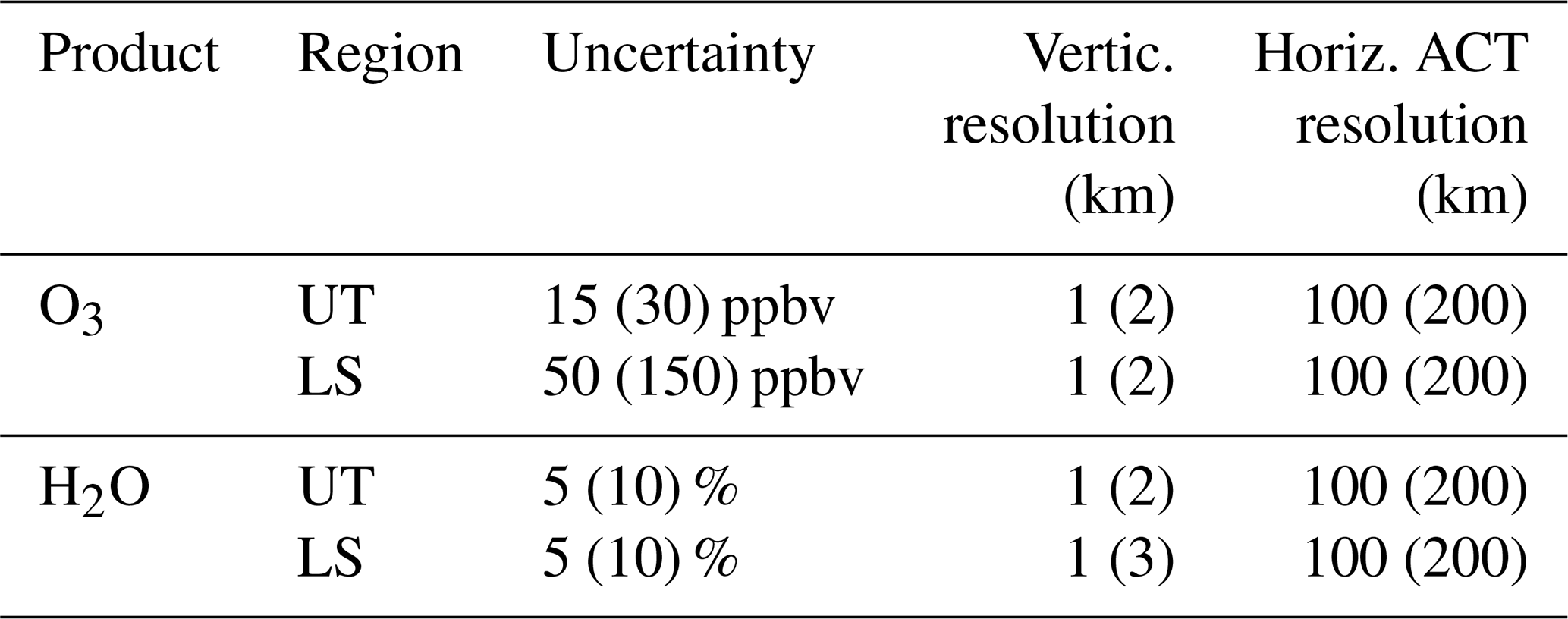
The Level-1 limb radiance spectra corresponding to multiple across-track spatial samples are averaged to reduce noise before Level-2 retrievals (see Sects. 4.4 and 4.5, and ESA, 2025a, Sect. 7.2.3). For O₃ and H₂O in the UTLS, the spectra are binned across-track to get a spatial resolution of 100 km. Considering a default swath of 400 km, CAIRT would thus retrieve L2 profiles along four orbit tracks spaced out by 100 km for O₃ and H₂O in the UTLS (this can change for other species or altitude region).

CAIRT builds upon the strong space heritage of infrared limb emission measurements established by the Michelson Interferometer for Passive Atmospheric Sounding (MIPAS) instrument onboard Envisat, which operated between 2002 and 2012 (Fischer et al., 2008). MIPAS was a FTS scanning instrument with several co-aligned detectors, covering different spectral ranges, providing one retrieved profile approximately every 400 km. Given its 50 km ALT resolution and its four tracks, CAIRT would retrieve ∼ 32 times more profiles than MIPAS, and ∼ 12 times more profiles than MLS which provides one profile every 167 km along the orbit track (see Sect. 5). If implemented, CAIRT would be the first infrared limb imager in space, building on the heritage of the Gimballed Limb Observer for Radiance Imaging of the Atmosphere (GLORIA), which has flown on balloons and aircraft since 2011 (Riese et al., 2014; Friedl-Vallon et al., 2014). Experience with the airborne demonstrator instrument GLORIA provides confidence that the estimated performance of the CAIRT concept are realistic.

3 The nature run

In this study, a CAMS control simulation is used as the nature run providing the synthetic truth state for ozone, water vapour and cloud. It is based on the Integrated Forecast System for COMPOsition (IFS-COMPO) cycle 47r3. The meteorological upgrade implemented in cycle 47r3 is described in Forbes et al. (2021), while the chemical scheme is summarized in Arola et al. (2022) and references therein. This cycle became operational in October 2021 but had been running as an experimental control simulation since March of that year.

Unlike the operational CAMS analyses, the control simulation does not assimilate either chemical or meteorological observations. However, its meteorology – including the specific humidity – is reinitialized every 24 h from the operational CAMS analyses at 00:00 UTC. The simulation employs a reduced Gaussian grid at TL511 horizontal resolution (approximately 40 km) with 137 vertical levels, providing a vertical resolution of about 400 m at 50 hPa, 300 m in the UTLS, and getting finer toward the surface.

In IFS-COMPO 47r3, ozone is represented using a detailed chemistry scheme in the troposphere and a linearized parameterization in the stratosphere (Flemming et al., 2015). For water vapour, we use the specific humidity field provided by IFS-COMPO. The control simulation was selected because its output is archived every 3 h, compared to every 6 h for the operational analyses. In this configuration, ozone is not constrained by any observations, whereas water vapour is indirectly constrained through the daily reinitialization of specific humidity from the CAMS analyses, within which this variable is assimilated in the troposphere.

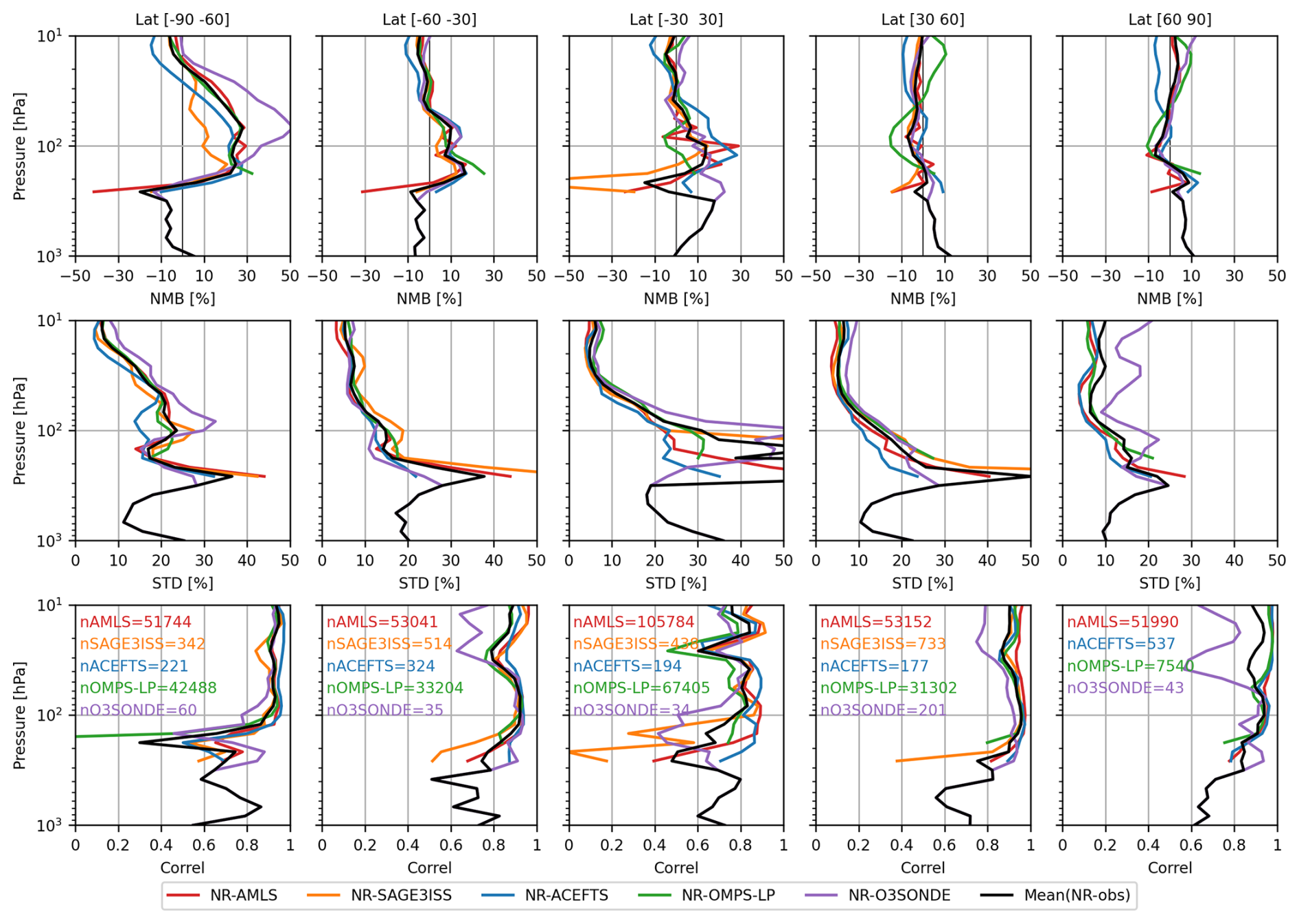
Figure 1 Comparison of ozone from the nature run (NR) CAMS control simulation against profiles from limb instruments and ozonesonde (see legend for colour code) during October 2021–December 2021 for five latitude bands (see title of each column). Statistical values shown are, from top to bottom: mean bias normalized by the mean of the CAMS profile (NMB), the associated standard deviation (NSD) and the correlation between CAMS and the observations (Corr). Also shown is the statistical comparison of the CAMS control simulation against the mean of all instruments (black line). The number of profiles used in each latitude band are given in the Correlation plots in row 3.

Ozone from the CAMS control simulation is routinely evaluated against a wide range of observational datasets by the CAMS Evaluation and Quality Control (EQC) service (see, e.g., Arola et al., 2022, and https://atmosphere.copernicus.eu/eqa-reports-global-services, last access 13 November 2025). Following the CAMS EQC methodology, ozone from the CAMS control simulation is interpolated at the profile geolocation of ozonesondes and a set of limb-sounding instruments: the Atmospheric Chemistry Experiment Fourier Transform Spectrometer (ACE-FTS) version 5.3 (Boone et al., 2023), MLS version 5.0 (Livesey et al., 2022), the Ozone Mapping and Profiler Suite Limb Profiler (OMPS-LP) onboard the S-NPP satellite, version 2.6 (Kramarova et al., 2024), and the Stratosphere Aerosol and Gas Experiment III onboard ISS (SAGE-III/ISS) version 6.0 (Wang et al., 2020). Statistical differences between CAMS interpolated profiles and these observations are displayed in Fig. 1 in five latitude bands for the period October–December 2021 (see Fig. 1). The rationale for selecting this period is provided in the following paragraphs. The statistical indicators shown are the normalized mean bias (NMB) between CAMS and the observations, the associated normalized standard deviation (NSD), and the correlation coefficient (CORR) between CAMS and the observations. NMB and NSD use the mean values of CAMS for normalization.

In the stratosphere (above 100 hPa), except over the southern polar region, the agreement between the CAMS control simulation and both ozonesonde and satellite observations is generally good. The mean bias remains within ±10 %, the standard deviation of the difference is below 10 %, and the correlation typically exceeds 0.8. In the troposphere, the agreement is less good: comparisons with ozonesondes reveal positive biases between +10 % to +20 % in the tropics and biases within ±10 % at mid-latitudes. The standard deviation increases notably in the tropics, although the correlation remains between 0.5 and 0.8. While ozone from the operational CAMS analysis exhibits better agreement due to the assimilation of multiple satellite ozone retrievals, the quality of the control simulation is considered sufficient for the purposes of this study.

Figure 2 As Fig. 1 but for water vapour.

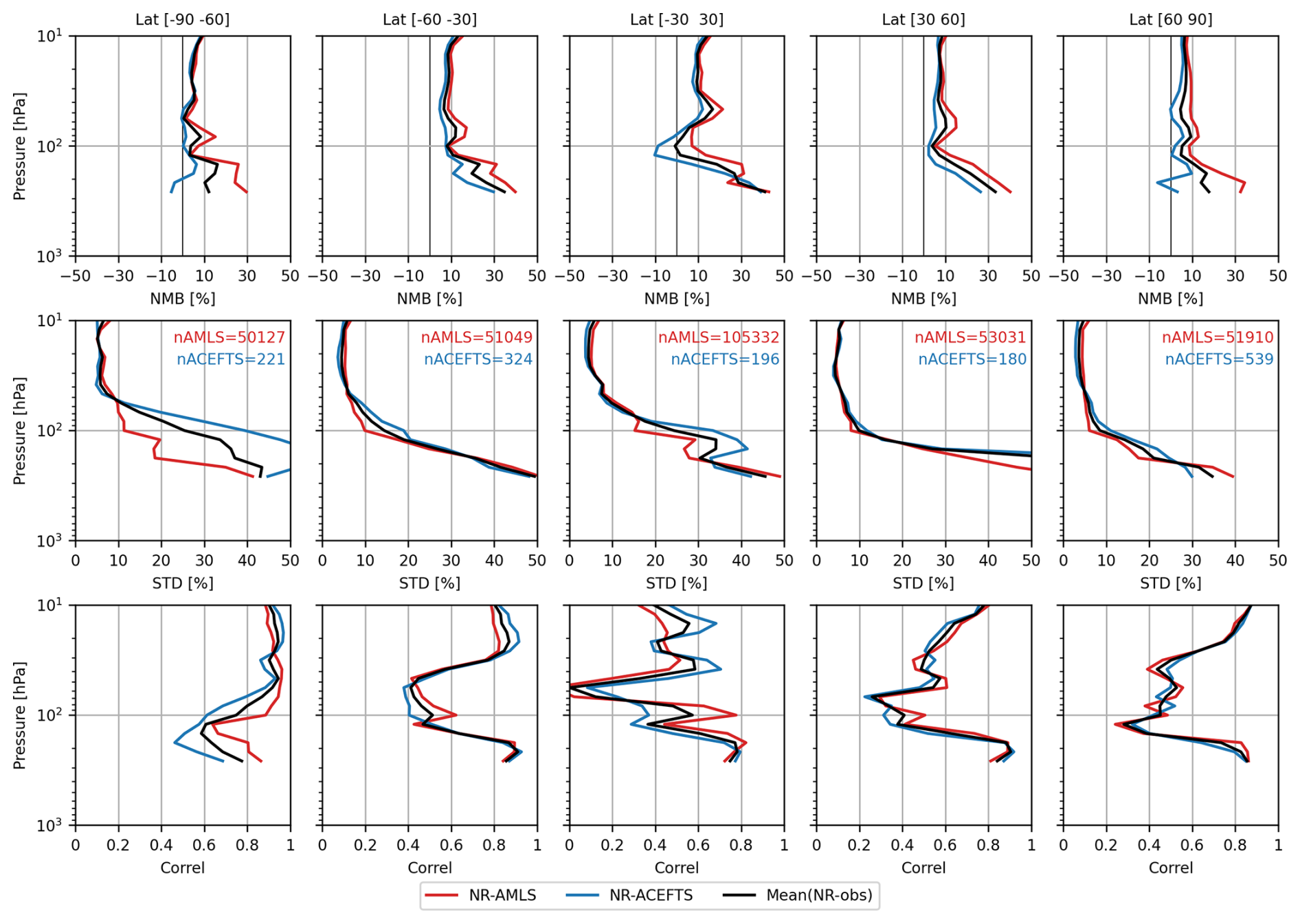
For specific humidity, major upgrades to the moist-physics parameterizations and the assimilation of satellite observations were introduced in IFS-COMPO cycle 47r3 (Forbes et al., 2021), reducing the stratospheric temperature bias by up to 50 %. Using the same evaluation methodology as for ozone, specific humidity from the CAMS control simulation was compared with measurements from two limb-sounding instruments (see Fig. 2). Because the stratospheric water vapour content increased by approximately 10 % following the Hunga eruption in mid-January 2022 (Millán et al., 2022), and since this source of water vapour is not represented in CAMS, the comparison was restricted to the October-December 2021 period.

In the stratosphere (above 100 hPa), the mean bias in specific humidity is positive, between 0 % and +10 %, with a standard deviation below 10 %. In the troposphere, both the mean bias and standard deviation increase with pressure, reaching approximately +30 % and 50 %, respectively, at 250 hPa. The correlation remains relatively high above 50 hPa and below 200 hPa, but decreases to around 0.5 between these pressure levels, except in the tropics near 50 hPa where it approaches zero. Nevertheless, as for ozone, the quality of the control simulation is deemed adequate for use in this study.

The CAMS control simulation is archived in the ECMWF MARS system, and the corresponding MARS parameters required for data retrieval are provided in the Code and data availability section at the end of this paper.

4 Simulating CAIRT observations

Simulating CAIRT Level-2 (L2) profiles from the nature run involves several steps, illustrated in Fig. 3. First, the satellite orbit must be simulated, i.e. the satellite position and velocity vectors are determined at a frequency consistent with the along-track sampling. Second, given the satellite position and velocity and the CAIRT viewing direction, the CAIRT retrieval grid is computed, providing the geolocation of the points observed by CAIRT. Third, the nature run is interpolated at the observed points, yielding the NR@L2 dataset.

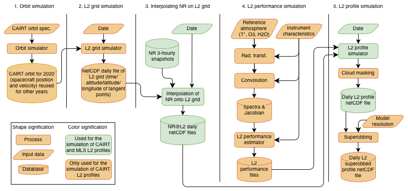
Figure 3 Processing chain used to simulate CAIRT and MLS Level-2 profiles. Processes in orange are only done for CAIRT while processes in green are done for CAIRT and MLS.

The performance characteristics of the L2 products, namely the averaging kernels and observational uncertainties, must also be simulated (step 4). Subsequently (step 5), the simulated L2 profiles are generated by convolving NR@L2 with the L2 performance characteristics. To account for the potential saturation of Level-1 (L1) spectra caused by the presence of clouds, cloud information is incorporated at this stage.

Because the number of CAIRT profiles is significantly larger than that of any existing limb-sounding instrument, direct assimilation into the BASCOE-EnKF system would lead to memory overflow. This is a well-known issue in data assimilation (DA), for which a common solution is the generation of superobservations (often referred to as superobbing in DA terminology), obtained by combining observations available at the same time within the same model grid cell.

All these steps are described in detail in the following subsections.

4.1 CAIRT orbit simulation

As mentioned in Sect. 2, one of the CAIRT requirements is to provide observations co-registrated with IASI-NG onboard MetopSG. The simulation of the CAIRT orbit (step 1 in Fig. 3) was thus performed using the MetOp-SG orbit specifications as a reference, with adjustments to the longitude of the ascending node to ensure that the MetOp-SG Nadir instruments and CAIRT sample the same air masses simultaneously (see Table 2). ESA's Earth Observation Mission Software was employed for the simulation (ESA, 2025a, b).

Table 2 Metop-SG and CAIRT orbit specifications.

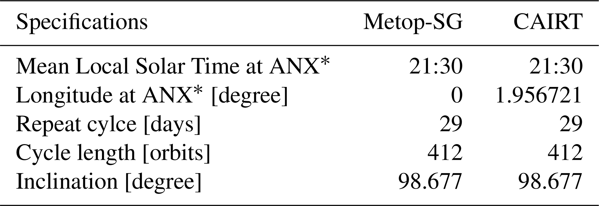
^∗ Ascending Node Crossing (the point on an orbit where the spacecraft crosses the Earth's equator from South to North).

An Orbit Scenario File was first generated (ESA, 2024, 2025c) to define the CAIRT orbit, which was subsequently used to compute the satellite position and velocity vectors with a propagation step of 7.56 s, corresponding to an along-track sampling step of approximately 50 km. The results of the orbit simulation were stored in an ASCII file (available on the CAIRT Zenodo repository, see Code and data availability section below) containing: the epoch of each propagation step (UTC), satellite position and velocity vectors in the Earth-Fixed Earth-Centered (EFEC) reference frame, latitude and longitude of the sub-satellite point, and the satellite's geodetic height.

4.2 CAIRT L2 geolocation simulation

Providing the orbit parameters, the second step is to set up the CAIRT L2 grids, i.e. the time and position where CAIRT L2 profiles will be available (step 2 in Fig. 3). This step is subdivided into two tasks. The first one is to estimate the geodetic tangent point (TP) at 30 km of altitude from a limb-viewing instrument looking backward on a polar orbit like CAIRT. An initial estimate is obtained from a spherical-Earth approximation, which provides a simple analytic relationship between spacecraft altitude, viewing geometry, and desired TP altitude. This initial value slightly overestimates the TP altitude when Earth's oblateness is considered, and it is therefore refined iteratively until the resulting TP altitude matches the requested value within a tolerance of 1 meter.

CAIRT being an imager, several profiles on parallel tracks will be retrieved at the same time and the second task is to find the geolocation of these profiles. For O₃ and H₂O in the UTLS, the ACT sampling has been set to 100 km (see Sect. 2, while for temperature, the goal and threshold are, respectively, 25 and 50 km ACT). With a swath of 400 km, this will provide four profiles per image. Their geolocations are computed left and right to the TP at 30 km and in a perpendicular plane to the LoS.

4.3 Interpolation of the nature run on the L2 grid

The regridding of NR onto the CAIRT L2 grid (step 3 in Fig. 3) is performed using a subset of the BASCOE system, namely its BASCOE-MAO mode (Model At Observation). As a data assimilation system, BASCOE includes routines to read model fields and observation files, as well as an observation operator to interpolate model fields to the geolocations of the observations. In its MAO configuration, model fields are taken from snapshot files rather than being simulated by the BASCOE model. In this procedure, the 3-hourly CAMS snapshot fields are linearly interpolated in time and space to the geolocations of the CAIRT tangent points. This is the same procedure used in the CAMS EQC project to validate CAMS stratospheric ozone analyses and forecasts.

4.4 CAIRT L2 Performance Simulation

To simulate CAIRT L2 profiles, the L2 performance must be estimated (step 4 in Fig. 3), including the averaging kernels and uncertainties under different atmospheric conditions. This simulation should balance computational efficiency with sufficient complexity to provide a realistic representation of the observing system's (including the instrument's) performance.

A parametric approach based on linear retrieval simulations is employed, allowing efficient generation of large volumes of emulated L2 data while realistically representing the instrument performance. This approach will be presented in Funke et al. (2026) and is summarized below.

4.4.1 Climatology generation

A climatology of the atmospheric conditions encountered by CAIRT was created for all relevant parameters that influence spectral signatures in CAIRT's measurement range (Errera et al., 2026). This includes O₃, H₂O, CO₂, temperature, and other trace gases. To represent variability, the climatology was computed for four representative months corresponding to different seasons (January, April, July, and October), five latitude bands (90–70° S, 55–35° S, 20° S–20° N, 35–55° N, and 70–90° N), the two overpass local times (09:30 and 21:30), and 201 vertical levels (0–200 km with 1 km spacing).

Since no single atmospheric model or dataset provides all relevant trace gases across the vertical domain between 5 and 115 km, this climatology was created by blending outputs from multiple simulations from multiple models. For ozone and water vapour in the UTLS, the climatology is based on the Whole Atmosphere Community Climate Model (WACCM; Gettelman et al., 2019) in its ACOM configuration (Atmospheric Chemistry Observations and Modeling), which has been operational since August 2019. The period considered for climatology generation was October 2019–October 2022, which was the longest available period at the time of the CAIRT Phase 0 project.

4.4.2 Radiative transfer simulations

Using the climatology and the Karlsruhe Optimized and Precise Radiative transfer Algorithm (KOPRA; Stiller, 2000), an ensemble of radiance spectra and their Jacobians were computed at a fine spectral sampling of 5 × 10⁻⁴ cm⁻¹. Subsequently these spectra were resampled to 0.2 cm⁻¹ by convolution with a sinc-function representing an ideal Fourier-Transform spectrometer of 2.5 cm⁻¹ maximum optical path difference. Perturbations were included to account for uncertainties in instrument and atmospheric parameters which are described in ESA (2025a). The resulting spectra and Jacobians were then vertically and spectrally convolved with representative functions based on instrument specifications, including vertical sampling, the vertical System Energy Distribution Function (SEDF), and spectral apodization using the Norton–Beer–Strong function (Norton and Beer, 1976, 1977).

4.4.3 L2 performance estimation

For each of the different climatological conditions, L2 performance has been diagnosed based on the corresponding radiance spectra and Jacobians. Resulting output files include the two-dimensional (vertical and along-track) averaging kernels, decomposed random error covariance matrices representing measurement noise, and two Monte-Carlo ensembles of systematic error profiles (corresponding to across-track correlated and uncorrelated uncertainties, respectively). This computation employs a tomographic retrieval approach for limb observations as in Steck et al. (2005). Instrument specifications based on CAIRT's threshold uncertainty assumptions – including calibration uncertainty, calibration cycle, and systematic uncertainty – were incorporated, along with error propagation from temperature and line-of-sight retrievals in the O₃ and H₂O profiles.

In this paper, systematic errors are every type of error that are not strictly random. These include radiometric calibration errors ((1) offset and (2) scaling), (3) pointing knowledge, (4) spectral responses function (i.e., the apodized instrumental line shape), (5) system energy distribution function (i.e., the spatial response of the optical system to a spectrally uniform point source), (6) systematic uncertainties due to imperfect knowledge on the CO2 vertical distribution and (7) non-LTE related kinetic rates. Systematic errors (3) to (7) are correlated in the across-track direction, while errors (1) and (2) are uncorrelated in that direction.

4.5 CAIRT L2 Profiles Simulation

4.5.1 Profile simulation

CAIRT L2 profiles are simulated for a given date using the NR@L2 daily file and the L2 performance file (step 5 in Fig. 3). The simulator interpolates the L2-estimated two-dimensional (vertical and along-track) averaging kernels and errors to the time and location of each CAIRT L2 profile. The NR@L2 profiles are then convolved with the interpolated averaging kernel matrices and randomly perturbed in a manner that preserves spatial error correlations as follows:

$$\begin{array}{}\text{(1)}& {\mathit{y}}_{\mathrm{l}\mathrm{2}}=\mathbf{A}{\mathit{y}}_{\mathrm{n}}+(\mathbf{I}-\mathbf{A}){\mathit{y}}_{\mathrm{a}}+{\mathit{ϵ}}_{\mathrm{rnd}}+{\mathit{ϵ}}_{\mathrm{sys}\mathrm{\_}\mathrm{corr}}+{\mathit{ϵ}}_{\mathrm{sys}\mathrm{\_}\mathrm{uncorr}}\end{array}$$

where y_l2 is a simulated L2 profile, y_n is a chunk of NR@L2 profiles on the CAIRT grid spanning ±1900 km in the along-track dimension, centered on the tangent point of y_l2, and A is the CAIRT averaging kernel matrix corresponding to the geolocation of that chunk. The term y_a represents the a priori profile, and I is the identity matrix.

The perturbation ϵ_rnd is obtained by multiplying a Gaussian random number field with the factorized random error covariance matrix. The profiles ϵ_{sys_corr} and ϵ_{sys_uncorr} represent the systematic error contributions, corresponding to the along-track correlated and uncorrelated components, respectively.

In our computation, y_a has been set to zero such that the regularization (Tikhonov first order) acts as a simple smoothing constraint without any influence of the a priori profile shape. Moreover, our computation of CAIRT L2 profiles does also store the different terms of Eq. (1) allowing to remove the contribution of some of them and test their impact in the OSSE (see Sect. 7).

4.5.2 Cloud masking

The influence of clouds on the simulation of L2 profiles was also taken into account. Clouds can affect spectra and introduce artifacts that can significantly degrade the quality of the L2 products. Therefore, in infrared retrievals, spectra strongly affected by optically thick clouds are typically excluded prior to retrieval in order to avoid instabilities and errors in the retrieval of trace-gas concentrations.

CAIRT adopts a two-dimensional (2D, vertical × ALT) tomographic retrieval approach. On the one hand, this allows information at a given location to be retrieved from multiple viewing directions. On the other hand, lines of sight with tangent points outside the cloud location may still intersect the cloud along their propagation path and therefore be affected by it.

The impact of thick clouds on the number of valid retrieval points has been studied by conducting 2D simulations of retrieval with a cloud in the line of sight. The cloud extends vertically from its top altitude to 5 km, and horizontally along the satellite track for 50 km, which corresponds to the along-track retrieval grid spacing. The procedure consisted of first removing all spectra whose lines of sight intersect the cloud volume, then computing the retrieval averaging kernels and identifying the grid points for which the diagonal elements of the averaging kernel fall below a specified threshold. This was repeated for clouds with different cloud-top heights.

Based on this analysis, a set of lookup-table masks was derived for different cloud-top altitudes and applied in the a posteriori filtering of L2 products. A scene is classified as cloudy when the cloud fraction from the CAMS dataset, interpolated at the corresponding L2 geolocation, exceeds 0.2. The L2 simulated profiles are thus filtered a posteriori using the masks derived from the cloud-impact analysis described above. This will be described in more details in Funke et al. (2026).

4.5.3 Superobservations

As previously mentioned, CAIRT will deliver substantially more profiles than existing limb instruments, e.g., approximately 12 times more than MLS. This number is too large to be handled directly by the BASCOE-EnKF system used in our OSSE. At each model time step, the system must invert a matrix whose size depends on the number of available observations multiplied by the ensemble size. With the default model time step of 30 min and an ensemble size of 20, this corresponds to a matrix with 6.6×10⁵ points to invert (i.e., 240 acquisitions × 4 tracks × 35 altitude levels from 5 to 40 km × 20 ensemble members). This exceeds the computational capacity of the BIRA-IASB server.

Reducing the model time step to 7.5 min decreases the matrix size by a factor of 4, making the computation feasible. However, this configuration produces noisy analysis increments, degrading the quality of the assimilation. This is a well-known issue in data assimilation, for which one common solution is the construction of superobservations (Eskes et al., 2003; Hoffman, 2018). In this approach, observations located within the same model grid cell at the same model time step are combined.

In our study, superobservations are computed as follows and illustrated in Fig. 4. Let λ_i and ϕ_i being the longitude and latitude of i=1…N L2 profiles available within a model time step and within the same model grid cell. Let y_i,l the corresponding L2 observations and e_i,l the associated L2 uncertainties where l=1…L is the vertical level index. Let us define M_l the number L2 profiles uncontaminated by cloud at level l, M_l≤N. For each level l, the L2 superobservation longitude Λ_l, latitude Φ_l, value s_l and uncertainty σ_l are computed as follows:

$$\begin{array}{}\text{(2)}& {\displaystyle }{\mathrm{\Lambda }}_l={\displaystyle \frac{\mathrm{1}}{M_l}}\sum _{i=\mathrm{1}}^{M_l}{\mathit{\lambda }}_i\text{(3)}& {\displaystyle }{\mathrm{\Phi }}_l={\displaystyle \frac{\mathrm{1}}{M_l}}\sum _{i=\mathrm{1}}^{M_l}{\mathit{\varphi }}_i\text{(4)}& {\displaystyle }{s}_l={\displaystyle \frac{\mathrm{1}}{M_l}}\sum _{i=\mathrm{1}}^{M_l}{y}_{i,l}\text{(5)}& {\displaystyle }{\mathit{\sigma }}_l=\sqrt{{\displaystyle \frac{\mathrm{1}}{M_l}}\sum _{i=\mathrm{1}}^{M_l}{e}_{i,l}^{\mathrm{2}}}\end{array}$$

Since only CAIRT L2 observations uncontaminated by clouds are included in this computation, the latitude and longitude of superobservations may vary with altitude.

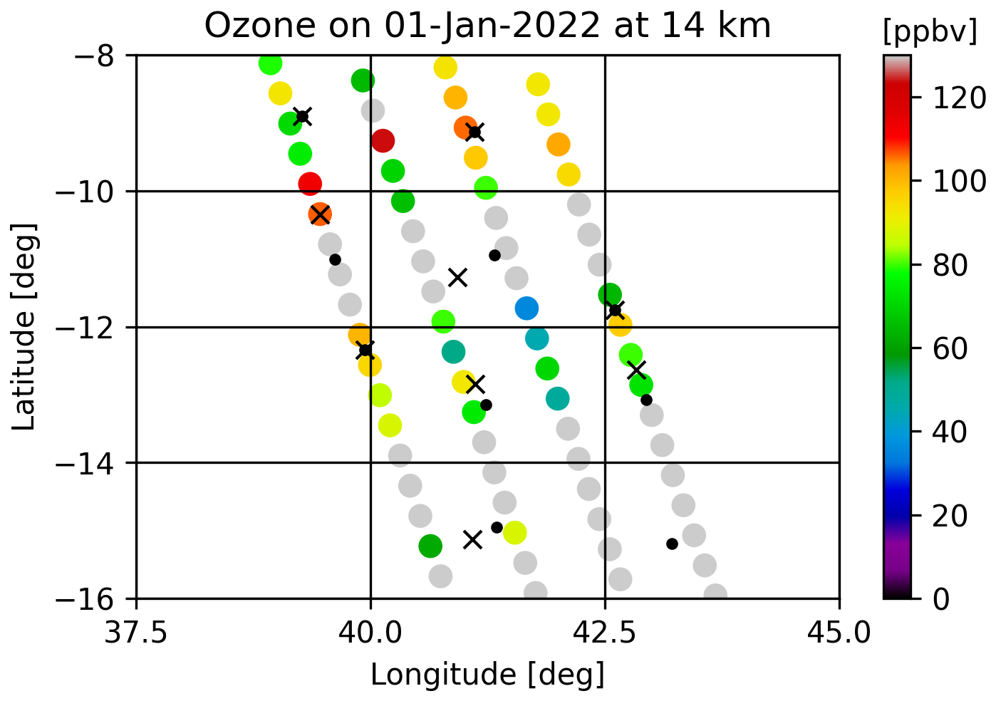
Figure 4 Coloured dots represent CAIRT L2 O₃ observations at 14 km on 1 January 2022. Gray dots are CAIRT L2 observations obscured by clouds when CAMS cloud fraction is greater than 0.2. The grid represents the BASCOE spatial resolution used in the control and assimilation runs. Superobservations will be the average values of valid CAIRT L2 observations within the same BASCOE grid point, located at the black crosses. Black dots would be the locations of superobservations if no cloud filtering were used.

If observation errors and correlations were perfectly represented, the use of individual observations or superobservations in data assimilation would produce identical analyses. In practice, however, superobservations reduce representativeness errors and mitigate the overweighting of dense, correlated data. As a result, the analyses typically differ slightly, often yielding smoother and more balanced fields (Duncan et al., 2024; Rijsdijk et al., 2025).

5 Simulating MLS observations

The computation of MLS simulated profiles differs from that of CAIRT profiles in that some of the required data are already available. This includes the geolocation of MLS profiles, the a priori profiles, the L2 error profiles, and the vertical averaging kernels. The MLS geolocation, a priori profiles, and L2 error profiles are obtained from MLS v5 daily observation files, while the MLS v5 vertical averaging kernels are provided for five latitudes and are independent of time and longitude.

The CAMS nature run is interpolated onto the MLS retrieval grid using BASCOE-MAO, as for CAIRT (see Sect. 4.5, and is then perturbed to produce the L2 profiles y_l2 as follows:

$$\begin{array}{}\text{(6)}& {\mathit{y}}_{\mathrm{l}\mathrm{2}}=\mathbf{A}{\mathit{y}}_{\mathrm{n}}+(\mathbf{I}-\mathbf{A}){\mathit{y}}_{\mathrm{a}}+{\mathit{ϵ}}_{\mathrm{p}}\end{array}$$

Here, y_n represents the nature run interpolated onto the MLS grid; y_a denotes the existing MLS a priori profiles corresponding to the MLS geolocation; A is the MLS vertical averaging kernel matrix; and I is the identity matrix. Note that MLS along-track averaging kernels have not been taken into account. The perturbation profile ϵ_p is a Gaussian random profile multiplied by the MLS L2 error profile provided in the MLS data files.

Simulated profiles are only assimilated within the vertical range of validity specified in Livesey et al. (2022). This report also defines criteria for accepting or discarding profiles based on the variables “estimated precision,” “quality,” “convergence,” and “status” provided in the MLS files. These criteria were used to flag entire profiles or portions of profiles, discarding measurements contaminated by clouds, particularly for O₃ (see discussion in the next section).

6 About Differences Between CAIRT and MLS

As previously mentioned, CAIRT will provide substantially higher sampling than MLS (or MIPAS) for O₃ and H₂O in the UTLS, delivering approximately 12 times more profiles. This is illustrated in Figs. 5 and 6e. Figure 6 compares various performance metrics for CAIRT and MLS: (a) random error, (b) systematic error, (c) vertical resolution, (d) horizontal resolution, and (e) number of available observations. For CAIRT performances discussed in Sect. 4.4, the displayed values correspond to January in the tropics. This provides a conservative view of the CAIRT performances compared to other latitudes (not shown). MLS performances are taken from the MLS v5 data quality document and are generally independent of latitude and season, except for the number of observations (Livesey et al., 2022).

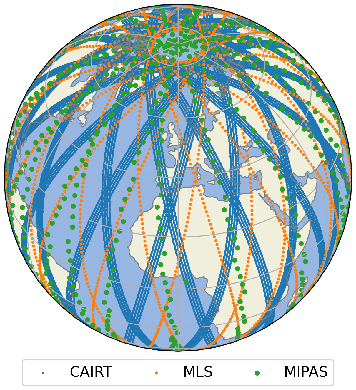
Figure 5 Illustration of CAIRT sampling for O₃ and H₂O in the UTLS compared to MLS and MIPAS. This is on 16 January 2022 for CAIRT and MLS, for the same day in 2011 for MIPAS.

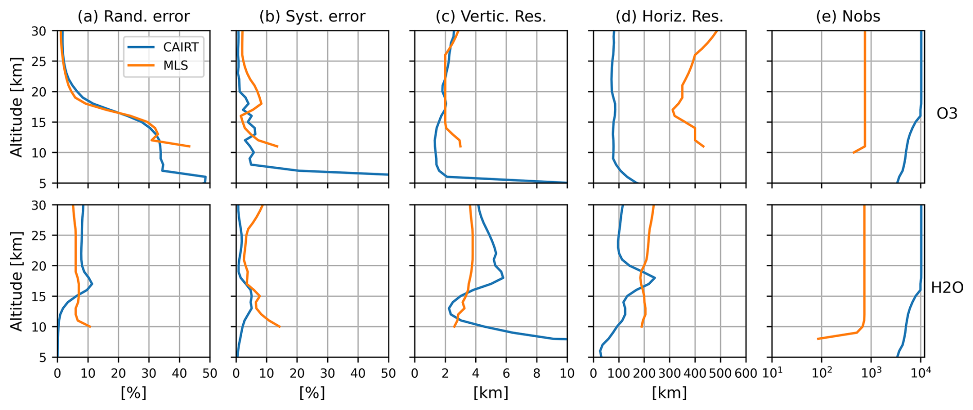
Figure 6 Performances of CAIRT (blue lines) and MLS (orange lines) for ozone (top line) and water vapour (bottom line). From left to right: random error, systematic error, vertical resolution, horizontal (along track) resolution and average number of valid observations for the period October 2021–February 2022. CAIRT performances are for January in the tropics. MLS performances do not depend on the latitude region or the season. While MLS data quality document provides 2σ systematic error, 1σ random and systematic error are given here for both instruments.

For O₃, CAIRT and MLS exhibit comparable random errors, whereas for H₂O, MLS shows slightly smaller (i.e., better) random errors (Fig. 6a). For O₃, CAIRT systematic errors exceed 50 % below 7 km in the tropics; consequently, CAIRT O₃ observations below this altitude have not been assimilated. The vertical resolutions of both instruments are comparable for O₃, while MLS generally exhibits better vertical resolution in the stratosphere for H₂O (Fig. 6c). For both species, CAIRT achieves superior horizontal resolution (Fig. 6d). The number of available observations for January is shown in Fig. 6e; the decrease with decreasing altitude is due to the presence of clouds.

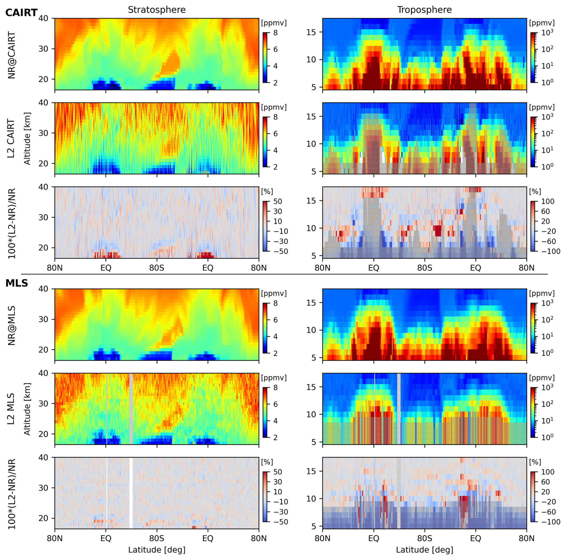
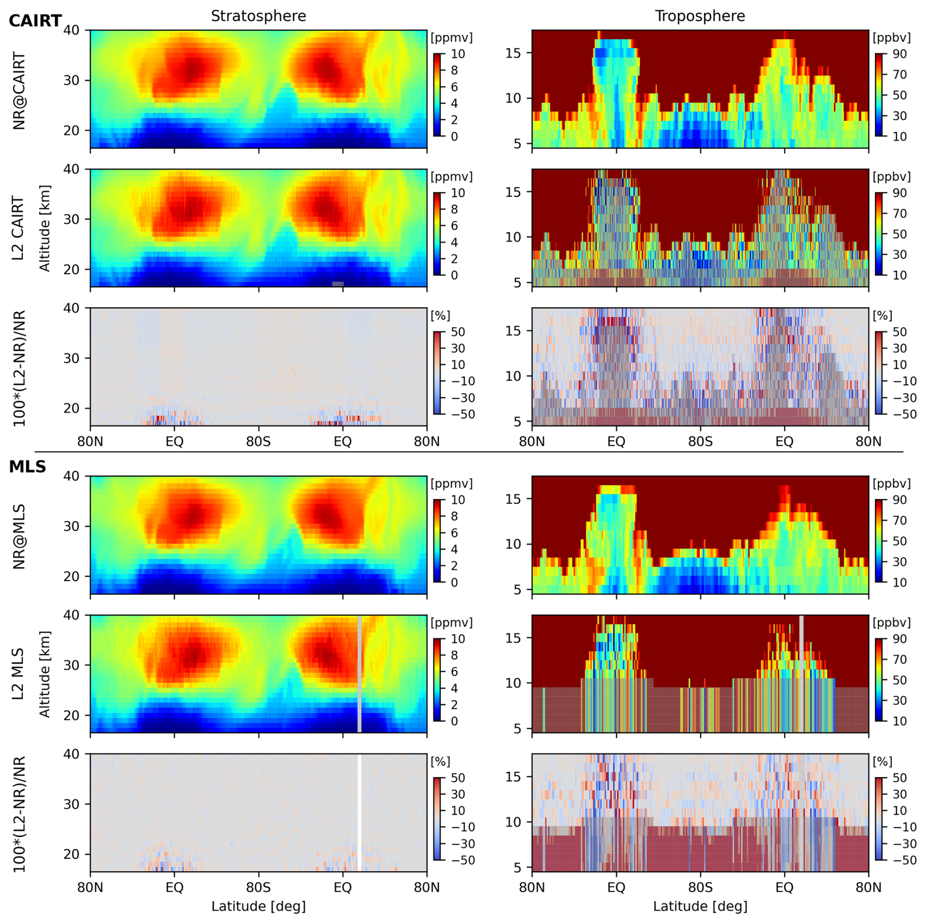
Figure 7 (Top panels) Ozone along the first complete CAIRT orbit on 15 December 2021 for track 2. The top line shows the CAMS nature run interpolated on the CAIRT orbit in the stratosphere (left, in ppmv) and the troposphere (right, in ppbv). The second line shows the CAIRT simulated L2 observations and the third lines the difference between L2 observations and the nature run (in %, normalized with the nature run). Gray areas denote observations obscured by clouds or rejected below 7 km due to a too-large systematic error. (Bottom panels) As top for MLS for the closest orbit to CAIRT on the same date. Here, invalid MLS data are indicated by the gray area.

Figure 7 compares CAMS ozone with the corresponding L2 simulated observations for CAIRT and MLS along an orbit on 15 December 2021. Note that CAIRT and MLS orbits differ in time and position; therefore, this comparison provides only a qualitative indication of their differences. In the stratosphere, CAIRT and MLS observations closely match the original CAMS data, whereas in the troposphere the agreement is weaker. In the tropics, a large portion of CAIRT data below 15 km is rejected due to clouds, whereas MLS is less affected. This difference arises from the measurement techniques, as microwave observations (MLS) are less sensitive to clouds than infrared (CAIRT). Conversely, CAIRT provides more valid observations than MLS at mid and high latitudes. Similar patterns are observed for H₂O (see Fig. 8).

Figure 8 As Fig. 4 but for water vapour. Note the logarithmic colour bar in the troposphere.

7 Control and assimilation runs

Control and assimilation experiments were conducted with the BASCOE system (Errera et al., 2021), driven by ERA5 winds and temperatures. The simulations employed a horizontal grid of 91 latitudes by 144 longitudes (approximately 250 km horizontal resolution) and 51 vertical levels, with a vertical resolution of about 1.2 km at 50 hPa, 1 km in the UTLS, and decreasing toward the surface. This spatial resolution is considerably coarser than that of the nature run (see Sect. 3).

In the stratosphere, BASCOE, similarly to CAMS, uses a linearized ozone chemistry scheme, although the two systems are constrained by different climatological data. In the troposphere, BASCOE applies the same linearized chemical formulation as in the stratosphere, whereas CAMS employs a comprehensive tropospheric chemistry scheme (see Sect. 3).

For the experiments presented in this study, BASCOE does not account for any chemical processes involving water vapour. To prevent an unrealistic transport of tropospheric water vapour into the stratosphere, condensation is approximated by limiting the water vapour partial pressure to the saturation vapour pressure of water ice (Murphy and Koop, 2005). Consequently, the BASCOE and CAMS configurations and simulations exhibit substantial differences in their treatment of both O₃ and H₂O.

Table 3 Summary of model simulations and data assimilation experiments used in this study.

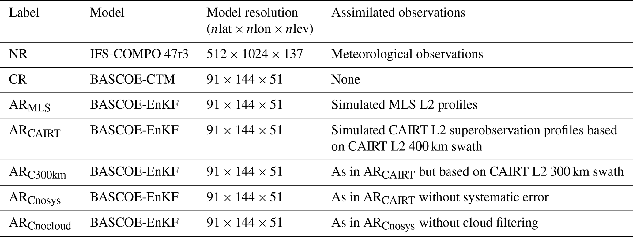
Six BASCOE experiments were performed, as summarized in Table 3. The first is a control run (CR) using the BASCOE Chemistry Transport Model (CTM) without data assimilation. The five other experiments are all assimilation runs using the BASCOE Ensemble Kalman Filter (ENKF). The first assimilation run is constrained by the simulated MLS profiles (AR_MLS). The additional assimilation runs were conducted using different simulations of CAIRT superobservation profiles. One experiment assumes a 400 km swath (AR_CAIRT), which corresponds to the default CAIRT configuration adopted during the Phase A study, another experiment assumes a 300 km swath (AR_C300km), representing the threshold value for CAIRT swath. Since the simulated MLS profiles do not include any systematic error, an additional assimilation run was performed with CAIRT simulated superobservation profiles with a 400 km swath where the contribution of systematic errors in the L2 profiles was excluded. Finally, to assess the potential impact of clouds, a fifth assimilation run (AR_Cnocloud) was carried out using the simulated CAIRT superobservation profiles with a 400 km swath, excluding the contribution of systematic error and cloud filtering.

The control run was initialized from the nature run on 15 August 2021, whereas all assimilation runs were initialized on 15 September 2021 from the control run. All simulations are evaluated against the nature run for the period from October 2021 to February 2022, allowing for a 15 d spin-up period for each assimilation experiment.

8 Results

CAIRT data help to improve the representation of ozone and water vapour, as illustrated in Fig. 9. The ozone distribution is shown at 7 km during a tropopause fold event above Europe, which is well represented by both the AR_CAIRT and AR_MLS assimilation runs, effectively correcting the bias present in the control run. One can also see the strong constraint provided by CAIRT observations, which substantially – though not completely – reduces the negative bias of the control run outside the tropopause fold region, and to a greater extent than MLS data. Similarly, CAIRT observations also provide a significant constraint, comparable to that of MLS, in the representation of water vapour at 12 km.

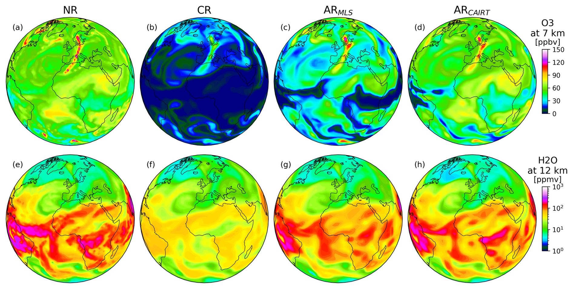
Figure 9 (a–d) Ozone distribution [ppbv] at 7 km of altitude on 3 December 2021 at 0 UT for (from left to right) the reference nature run (NR), the control run (CR), the MLS assimilation run (AR_MLS) and the CAIRT assimilation run (AR_CAIRT). (e–h) As top but for H₂O at 12 km of altitude.

8.1 Ozone

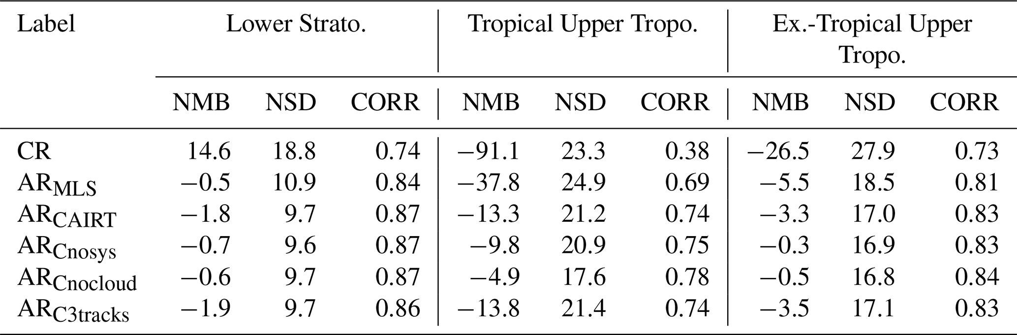
Figure 10 shows the statistical differences between the nature run and the various BASCOE runs for the period October 2021–February 2022 (five months), as a function of latitude and altitude for ozone. The statistics displayed are the normalized mean bias (NMB) between NR and {CR,AR}, the associated normalized standard deviation (NSD), and the correlation coefficient between NR and {CR,AR}. NMB and NSD use the mean values of NR for normalization. Before computing these statistics, the nature run was downgraded to the spatial resolution of the BASCOE runs. Table 4 provides the values of NMB, NSD and the correlations for all the experiments in three atmospheric regions: the lower stratosphere, the tropical upper troposphere and the extra-tropical upper troposphere.

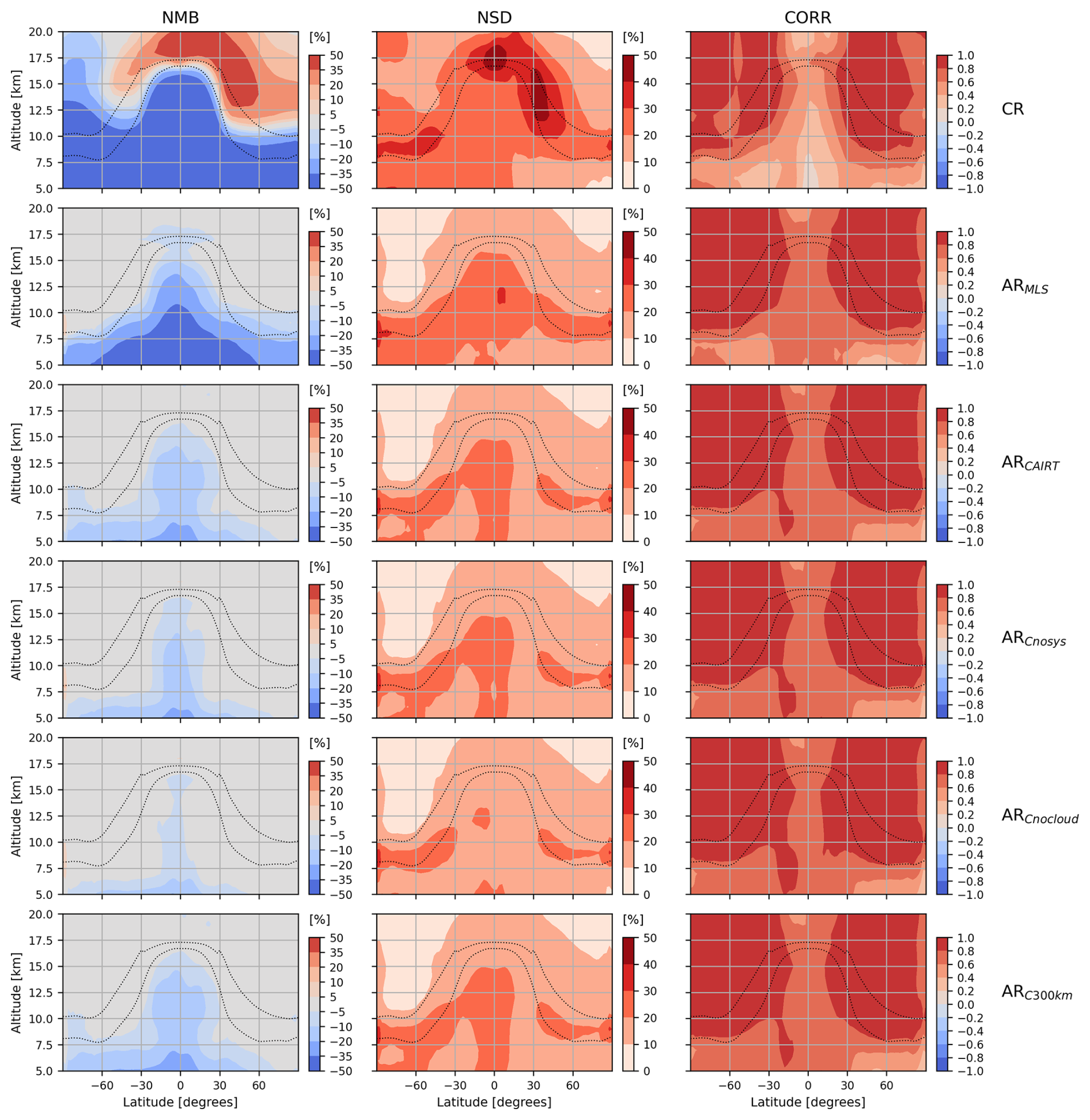
Figure 10 (Left column) Zonal mean of the mean bias (NR-{CR,AR}) normalized by the mean of NR (NMB, in %) for ozone and the period October 2021–February 2022. Each line corresponds to a different BASCOE experiment labelled at the right. (Middle column) The zonal mean of the associated normalized standard deviation (NSD, in %) of the differences shown in the left column. (Right column) The correlation between the nature run and the BASCOE runs.

Table 4 Mean values of the NMB (%), NSD (%) and CORR for O₃ in three atmospheric regions of Fig. 10: (1) the lower stratosphere defined by altitude between 18 and 20 km at all latitudes, (2) the tropical upper troposphere defined by altitude between 7 and 12 km and latitudes between ±20°, and (3) in the extra-tropical upper troposphere defined by altitude between 7 and 12 km and latitudes poleward ±30°.

As shown in Fig. 10, there are large differences between the control and nature runs: the BASCOE ozone chemistry predicts lower ozone concentrations in the stratosphere and higher ozone in the troposphere. Assimilating MLS data enables the BASCOE system to largely remove the ozone bias in the stratosphere and the tropopause region, accompanied by a strong reduction in the standard deviation and a significant increase in correlation compared to the control run. In the troposphere, while a large part of the control run bias is eliminated and the correlation with the nature run increases, a residual bias of about −38 % remains in the tropical upper troposphere (see Table 4).

The situation improves markedly when CAIRT observations are assimilated. The bias in the tropical upper troposphere decreases to −13 %, representing a clear improvement compared to MLS. The standard deviation of the differences and the correlation coefficients are also slightly improved when assimilating CAIRT rather than MLS data.

Since the simulation of MLS data does not include systematic error, an additional assimilation run using CAIRT simulated data without the contribution of systematic error was performed to ensure a fair comparison between both instruments. This configuration shows a substantial improvement in the bias in the tropical upper troposphere (−10 %) compared to AR_CAIRT, with the remaining bias mainly attributable to data scarcity and random error. When the cloud mask is disabled – thus including all profiles, even those excluded by clouds – and excluding the systematic error, the bias further decreases to −5 %, as shown by experiment AR_Cnocloud. Finally, reducing the swath width to 300 km does not significantly affect CAIRT's capability to observe ozone in the UTLS (see experiment AR_C300km in Fig. 10 and Table 4).

These results confirm the capability of CAIRT to provide valuable ozone information from the stratosphere down to about 7 km in the upper troposphere.

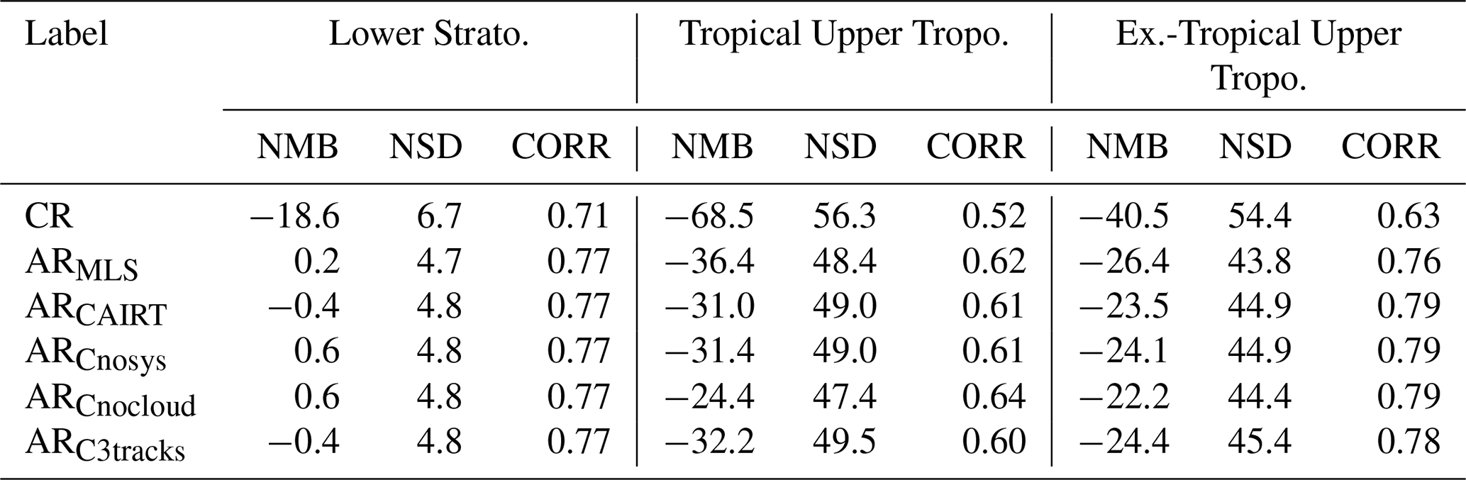
Table 5 As Table 4 but for H₂O where the troposphere differs in the altitude definition: the tropical upper troposphere altitude is defined between 10 and 16 km while the extra-tropical upper troposphere is defined between 8 and 14 km.

8.2 Water vapour

Figure 11 and Table 5 shows the statistical differences between the nature run and the other BASCOE runs, this time for water vapour. As for ozone, large discrepancies are observed between NR and CR. The improvements due to data assimilation are comparable in the lower stratosphere for all assimilated datasets: the bias is almost completely eliminated, and the standard deviation and the correlation are substantially enhanced. In the tropical and extra-tropical upper troposphere, all assimilation experiments show a reduction in bias and standard deviation, and a larger correlation, than the control run. Nevertheless, the biases are still significant (e.g. −36 % for AR_MLS and −31 % for AR_CAIRT in the tropics), the standard deviation larger than around 45 %, and correlation remains lower than 0.8 in the tropics. AR_CAIRT displays a lower bias than AR_MLS it the tropical and extra-tropical upper troposphere by a few %, both experiments providing comparable standard deviation and correlations. The results of experiments AR_Cnosys agree very well with those of AR_CAIRT indicating that the systematic error does not have a large impact on CAIRT H₂O profiles. Comparing the results between AR_Cnocloud and AR_CAIRT indicate that the 7 % of negative bias in the tropical upper troposphere is due to the presence of clouds. As for ozone, reducing the CAIRT swath to 300 km does not noticeably reduce the constraint of CAIRT on the BASCOE system.

Figure 11 As Fig. 10 but for water vapour.

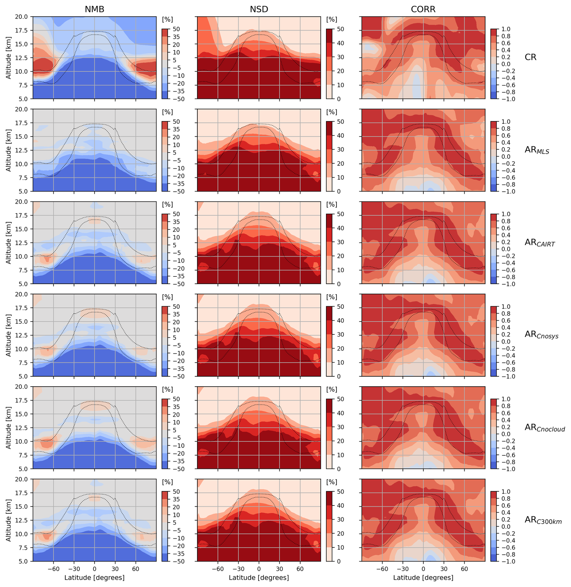
Compared to ozone, the constraint of CAIRT water vapour observations on the BASCOE system is weaker in the troposphere. This is likely due to the limited representation of water vapour physical processes in BASCOE. The condensation scheme implemented in BASCOE successfully produces a dry tropopause but removes too much water vapour in the mid-troposphere, resulting in a dry bias across all BASCOE experiments. Nevertheless, the primary objective of CAIRT water vapour profiles is to reduce the temperature bias in the UTLS in NWP systems, thereby improving forecast quality. In the troposphere, NWP systems already benefit from humidity observations provided by nadir-viewing satellite instruments and radiosondes.

9 Conclusions

This study evaluated the added value of ozone and water vapour profiles from the proposed satellite limb instrument CAIRT, designed to observe the temperature and composition of the middle atmosphere. The evaluation was conducted through an Observing System Simulation Experiment (OSSE) using an IFS model simulation as the nature run and the BASCOE system to perform the control and assimilation runs. CAIRT observations were simulated through a comprehensive processing chain starting from the IFS model fields as the synthetic truth, and accounting for CAIRT's orbit, geographical coverage, cloud contamination, spatial and spectral resolution, error budget, and superobservation strategy. For comparison, MLS profiles of ozone and water vapour were also simulated from the same IFS synthetic truth and assimilated by BASCOE, to assess the relative added value of CAIRT against an existing limb sounder.

For ozone, the OSSE results show that CAIRT can provide valuable information down to the mid-troposphere. Compared with the nature run, the BASCOE control run exhibits a positive bias above the tropopause and a negative bias in the troposphere exceeding ±50 %. Assimilating either MLS or CAIRT observations reduces the bias to within ±2 % in the lower stratosphere.

In the troposphere, MLS assimilation significantly reduces the control run bias, but a notable residual remains (−5 % in the extra-tropics to more than −35 % in the tropical lower troposphere). CAIRT data provide a stronger constraint, reducing the bias below −5 % in the extra-tropics and below −15 % in the tropics. Additional runs indicate that the remaining bias in the tropical troposphere is due to the presence of cloud. Furthermore, reducing the CAIRT swath from 400 to 300 km has little impact, suggesting that a narrower swath could be implemented if required by technical constraints without significant loss of performance.

For water vapour, CAIRT and MLS provide useful information in the lower stratosphere, reducing the bias and standard deviation to un-significant values. In the upper troposphere, while the bias and standard deviation remains significant (e.g. larger biases than −30 % for both instruments in the tropics), the improvement against the control run is large in all statistical indicator. As for O₃, reducing the swath to 300 km does not significantly affect CAIRT's ability to constrain the UTLS. Overall, these results indicate that CAIRT could deliver high-quality water vapour profiles suitable for constraining the UTLS region providing invaluable data to improve NWP systems.

This OSSE therefore demonstrates that CAIRT data are capable of meeting the mission's scientific objectives in the UTLS, particularly by improving the characterization of vertical gradients and small-scale structures of ozone and water vapour across the tropopause. Such capabilities directly support CAIRT's overarching goal of advancing our understanding of the coupling between atmospheric composition, circulation, and climate.