Super-resolution localization and quantification of SO₂ emissions over India using TROPOMI observations

India has high sulfur dioxide (SO₂) emissions, primarily due to its extensive coal-fired power sector. SO₂ column observations from Sentinel-5P Tropospheric Monitoring Instrument (TROPOMI) enables observation-based emission estimates using inversion techniques. Among inversion methods, the flux-divergence method is particularly sensitive to point source emissions and well-suited for estimating SO₂ emissions in India. However, when applied to satellite observations, this method tends to spatially spread calculated emissions into neighboring grid cells around the source. This spreading effect weakens the emission signal at the exact source location, making precise quantification of emissions more difficult. In this paper, we design a sharpening algorithm to reverse the spreading and sharpen the emission signals while conserving total mass of the emissions. We apply the algorithm on gridded SO₂ emissions at a high spatial resolution of 0.025° × 0.025° (≈ 2.5 km × 2.5 km) derived from TROPOMI observations that have a typical mean footprint size of 6.0 km × 6.0 km. After sharpening, the effective spatial resolution of the emissions matches the grid cell resolution. Emissions from point sources increase at their exact locations, while emissions in neighboring grid cells decrease. In the resulting SO₂ emission inventory, about 80 % of coal-fired power plants with capacities above 100 MW are detected at their correct location, while the remaining 20 % fall below the detection threshold. The detected power plants account for 99 % of India's total coal-based power generation. We also identify twenty two previously unreported SO₂ point sources, including coal-based thermal power plants, cement factories, crude oil production facilities, chemical fertilizers factory, and copper, steel, and aluminum industries. This sharpening algorithm improves emission detection and can also be extended to other pollutants emitted by point sources to enhance the accuracy of emission inventories.

1 Introduction

SO₂ is a reactive gas-phase pollutant in the atmosphere. It can react with hydroxyl radicals to form sulfuric acid (H₂SO₄), or with hydrogen peroxide and ozone to form sulfate (SO${}_{\mathrm{4}}^{\mathrm{2}-}$) in cloud droplets (Seinfeld, 1998). Both SO₂ and particulate SO${}_{\mathrm{4}}^{\mathrm{2}-}$ have harmful effects on human health and the environment. Exposure to SO₂ increases the rate of respiratory illness (Orellano et al., 2021; Tomić-Spirić et al., 2021). The sulfuric acid rain acidifies the soil and water ecosystem and damages buildings (Singh and Agrawal, 2007; Bhargava and Bhargava, 2013). SO${}_{\mathrm{4}}^{\mathrm{2}-}$ particles also promote cloud formation by increasing cloud condensation nuclei, thereby affecting regional and global climate system (Arnold, 2006; Feldman et al., 2012).

Atmospheric SO₂ originates from both natural and anthropogenic sources. Natural sources include volcanic eruptions and passive degassing (Eisinger and Burrows, 1998; Oppenheimer et al., 2011). Major anthropogenic sources include coal-based power plants, metal smelting and refining, and other coal-combustion activities (Klimont et al., 2013; Šerbula et al., 2014; Kuttippurath et al., 2022; Kang et al., 2019). In rapidly developing countries like India, SO₂ emissions are strongly linked to thermal power generation (Chakraborty et al., 2008; Nazari et al., 2010; Yadav and Prakash, 2014). Over the past two decades, India's thermal power capacity has increased substantially, from 7.4 × 10⁴ to 2.4 × 10⁵ MW (Patel, 2024). India has become the world's largest SO₂ emitter since 2016 (Li et al., 2017a, b) due to emissions from coal-based power plants. Despite this expansion, the country still faces power shortages with an estimated deficit of 8657 MW (Chan and Delina, 2023; Central Electricity Authority, 2023). The Global Energy Monitor recently reported a record high in request of new coal plant in India (GEM, 2025). SO₂ emissions are thus expected to keep rising as India remains heavily dependent on coal to meet growing energy demands driven by population growth and economic development. The widely-used bottom-up SO₂ emission inventory, Emissions Database for Global Atmospheric Research version 8 (EDGARv8), has been updated to 2022 (Crippa et al., 2024). However, its method first estimate emissions at the subnational level and then allocates the emissions to known point sources, which may not fully capture the emergence of new point sources and rapid emission changes. Therefore, a high-resolution, up-to-date SO₂ emission inventory is essential for tracking SO₂ emission changes and identifying new sources across the country.

Satellite instruments can monitor atmospheric SO₂ in the thermal infrared (IR) and ultraviolet (UV) band of the electromagnetic spectrum (Krueger et al., 2000; Eisinger and Burrows, 1998; Krueger, 1983; Bovensmann et al., 1999; Callies et al., 2000; Levelt et al., 2006; Veefkind et al., 2012; Taylor et al., 2018; Tournigand et al., 2020; Theys et al., 2021), enabling the estimation of SO₂ emissions through top-down methods. Two main inversion approaches, inverse modeling and mass balance methods, are commonly used to calculate SO₂ emissions from satellite observations. Inverse modeling methods estimate emissions of short-live gases like SO₂ by applying a correction to the bottom-up emissions, so that the simulated results align well with observations (Brasseur and Jacob, 2017). These methods depend on prior information to constrain and optimize the estimated emissions, and they are affected by uncertainties in transport models (Brasseur and Jacob, 2017; Qu et al., 2019; Wang et al., 2020). The dependency on prior information limits the ability of inverse modeling to detect new or unknown sources. In contrast, mass-balance methods, such as the plume fitting and flux-divergence methods, require less prior information without relying on chemical transport model. These physic-based methods mainly use satellite SO₂ measurements and wind field data for emission calculation. In the plume fitting method, the total SO₂ amount near an individual source is derived from fitting the plume of measured SO₂ density to a theoretical function. Emissions are then calculated by integrating the SO₂ amount and adding the estimated sink term, which is based on a constant decay rate derived from the plume function (Fioletov et al., 2011, 2013, 2015, 2016). However, using a fixed decay rate can affect the accuracy of the sink estimation, especially for gases like SO₂ that have variable lifetimes (Chen et al., 2025; Krol et al., 2024). The flux-divergence method has been used to estimate emissions of NO_x (Beirle et al., 2021; Cifuentes et al., 2025), CH₄ (Liu et al., 2021), CO₂ (Hakkarainen et al., 2022), and SO₂ (Chen et al., 2025). Compared to inverse modeling, this method is more time- and computational efficient, especially for generating emissions over large areas. Contrary to the plume fitting method, the divergence method generates regular gridded emissions.

Recently, the flux-divergence method for emission estimation has been further refined. It is based on the steady-state continuity equation and estimated emissions are the sum of advection and chemical sink terms (Beirle et al., 2019). A topography correction was later introduced to compensate for terrain-related biases in vertical column densities (VCDs) due to the vertical wind field (Sun, 2022), and has been applied to NO_x and CO emission estimation (Beirle et al., 2019; Sun, 2022). The topographic effects can also be accounted for by using total column densities (TVCDs) together with profile-weighted mean wind field for advection calculation (Koene et al., 2024). In addition, the previous studies also consider the full divergence (including both advection and wind divergence scaled by VCDs) for emission calculation. Sun (2022) demonstrates that the wind divergence term can be comparable in magnitude to a moderate emission signal. A corrected effective wind field is applied by Cifuentes et al. (2025) and Chen et al. (2025) to reduce topographic influences and derive the NO_x and SO₂ emissions.

The flux-divergence method can be applied for detecting and quantifying point source emissions because steep concentration gradients at point sources produce distinct divergence and thus emission signals (Beirle et al., 2019). In practice, however, the calculation of the gridded divergence, which involves concentration differences between neighboring grid cells, leads to the spatial spreading of emissions. This occurs because the spatial discretization distributes the divergence not only at the point source but also over the surrounding grid cells (Chen et al., 2025). Additionally, the finite resolution of the satellite measurements limits the capability to distinguish nearby point sources, thereby constraining the finest achievable resolution of the gridded divergence field. Reducing this spreading effect will improve both the accuracy and the spatial resolution of the emission inventory derived using the flux-divergence method.

In this study, we combine the divergence method and a sharpening algorithm to update the gridded Indian SO₂ emission inventory into an effective high spatial resolution of 0.025° × 0.025° (approximately 2.5 km × 2.5 km) using daily SO₂ observations from the Tropospheric Monitoring Instrument (TROPOMI) instrument (Veefkind et al., 2012; Theys et al., 2017). We use the same method as Chen et al. (2025) to estimate annual SO₂ emissions over India from December 2018 to November 2023. In this paper we describe a sharpening algorithm to remove the spreading of emissions, allowing the emissions to better reflect the true locations and strengths of sources. India is a good test case for this new approach due to its large amount of SO₂ point source emissions. We apply this sharpening algorithm to annual averaged emissions and the 5-year averaged emissions to demonstrate its performance for short-term and long-term periods. Section 2 describes the datasets used in this study. Section 3 presents the methodology, including the calculation of the spreading pattern and the implementation of the sharpening algorithm. In Sect. 4 we validate our method using model results and show the improved SO₂ emission results for India. Finally, Sect. 5 discusses the limitations and potential applications of the algorithm.

2 Datasets

2.1 Satellite observations and wind field datasets

For the divergence method a flux is derived by multiplying TROPOMI measured SO₂ vertical column density (VCD) gradients with the horizontal 2D wind field. The divergence of this flux is related to the emissions. We use the TROPOMI COBRA (Covariance-Based Retrieval Algorithm) SO₂ VCDs with a spatial resolution of 3.5 km × 5.5 km at nadir. The COBRA SO₂ VCDs represent SO₂ within the Planetary Boundary Layer (PBL), mainly associated with anthropogenic emissions. The COBRA retrievals can detect SO₂ concentrations of small anthropogenic sources with emissions of 8.0 Gg yr⁻¹ (Theys et al., 2021). We calculate the daily SO₂ divergence and subsequently compute seasonal averages for the period December 2018 to November 2023. To ensure good data quality, we exclude retrievals with a QA value below 0.5 or a surface height above 3 km (https://data-portal.s5p-pal.com/product-docs/SO2cbr/S5P-BIRA-PRF-SO2CBR_1.0.pdf, last access: 19 January 2026). Daily wind fields are taken from the daily operational 12h forecasts of the European Centre for Medium-range Weather Forecasts (ECMWF) at 0.25° × 0.25° resolution (https://www.ecmwf.int/en/forecasts, last access: 31 July 2025). Assuming SO₂ is vertically well mixed within the PBL, we use horizontal wind fields at half of the PBL height to represent PBL wind conditions. To reduce the artifacts from the simplified 2D wind field, especially over complex terrain, we correct the 2D wind fields for the wind divergence following the method of Bryan (2022).

2.2 Copernicus Atmospheric Monitoring Service (CAMS) Global Atmospheric Composition Forecasts

The monthly mean OH climatology is derived from the 5-year average from November 2018 to December 2023 using CAMS (Copernicus Atmospheric Monitoring Service) global forecast data (DOI: https://doi.org/10.24381/04a0b097; https://ads.atmosphere.copernicus.eu, last access: 9 September 2025) for chemical lifetime calculation. The forecast dataset is based on ECMWF's Integrated Forecast System (IFS), which assimilates and models the concentrations of more than 50 chemical species (such as SO₂ and OH), seven aerosol types, and various meteorological factors, all at a resolution of 0.4° × 0.4°. We derive the monthly mean OH climatology for the time period before the TROPOMI overpass time (13:30 local time) by averaging monthly OH concentration at 06:00 UTC (11:30 local time) within the PBL between 2018 to 2023, excluding days with extreme weather events, such as large-scale precipitation. The dry deposition lifetime is calculated by assuming a constant dry deposition velocity of 0.4 cm s⁻¹ in the atmosphere. Except for OH concentration, the SO₂ VCD within PBL and the wind field data in the mid-PBL layer from CAMS datasets are used for the method validation in Sect. 4.1.

2.3 SO₂ point source inventories for India

We use two datasets for validation over India. The first dataset is from the global power plants database maintained by the World Resources Institute (https://github.com/wri/global-power-plant-database, last access: 31 July 2025). This database provides the locations and power generation of 255 coal-based thermal power plants in India and is used to assess the positional accuracy of the point sources identified in our inventory. The second dataset is the global catalog of large SO₂ point sources from the Multi-Satellite Air Quality Sulfur Dioxide (SO₂) database, Long-Term L4 Global V2 (referred to as MSAQSO₂L4) (Fioletov et al., 2023). This catalog is based on SO₂ slant column density (SCD) data from two sources: the operational version 2 OMI and OMPS Principal Component Analysis (PCA) retrieval algorithm, and the TROPOMI Covariance-Based Retrieval Algorithm (COBRA) (Theys et al., 2021). Their emission estimates are derived using an exponentially modified plume fitting model. In total, the catalog identifies 92 SO₂ point sources in India. Both datasets are used to assess whether our method detects additional new point sources.

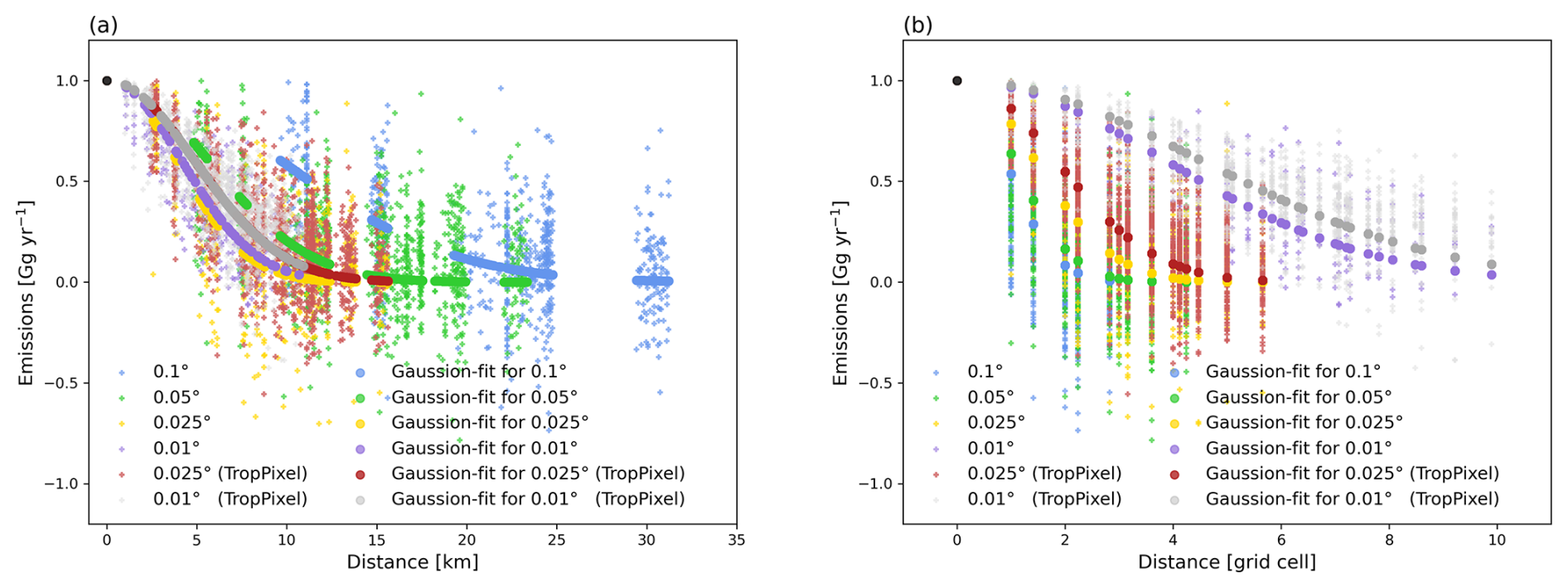
Figure 1 Variation of normalized SO₂ emissions with distance from the point source location, and the corresponding Gaussian-shaped fitting functions. Annual emissions from December 2022 to November 2023 are used for this figure. The emission distributions of 62 large and isolated point sources are used for fitting. The black point at (0,1) represents the location of the point source. The spreading of SO₂ emissions is fitted for the six cases in Table S1 in the Supplement.

3 Methodology

3.1 Divergence calculation

This full divergence calculation follows the method in Chen et al. (2025). Specifically, we use Eq. (S1) in the Supplement together with a corrected wind field to calculate SO₂ divergence. The wind is corrected using an iterative wind-divergence correction algorithm by Bryan (2022). As described in detail in Cifuentes et al. (2025) the impact of topography is clearly reduced, especially along coastal regions. We will calculate the emissions at various grid resolutions to test the effect of our sharpening: 0.1° × 0.1°, 0.05° × 0.05°, 0.025° × 0.025°, and 0.01° × 0.01°. We calculate the divergence on the TROPOMI pixels with rotated wind field following the method of Beirle et al. (2023) and then interpolate the results on the regular grid cells of 0.025° × 0.025° for the final emission estimates for the best results. See Sect. S1 for more details.

3.2 Determination of the spreading kernel

Since the spreading of emissions always takes place during the divergence calculation, we explore a sharpening method to further improve the emission resolution. We use a spreading kernel B to describe how the original true emission map X spreads to form the blurred derived emission map Y as expressed in the following equation:

$$\begin{array}{}\text{(1)}& \mathbf{Y}=\mathbf{B}\times (\mathbf{X}+\mathit{\epsilon }),\end{array}$$

where ε represents the noise on the original SO₂ emission map X. Now, we use the spreading kernel B to calculate the sharpening kernel. Kernel B can be derived from the derived emission distribution in the grid cells adjacent to the source location. Figure 1 shows the normalize derived SO₂ emissions as function of the distance from the point source location. To obtain a spreading kernel which represents the overall spreading pattern of point source emissions, we fit the emission variation around the large and isolated point sources in India using a Gaussian-shaped function. Figure 1a shows the SO₂ emissions and the corresponding Gaussian-shaped fitting functions as function of distance in kilometers. From Figs. 1a and S1 in the Supplement, we see that the emission resolution improves with finer grid cells, but gains become marginal once the grid is finer than the TROPOMI pixel size. Figure 1b shows the SO₂ emission as function of distance from the point source location, but with distance expressed in grid cells. Since we decide to derive the SO₂ emissions based on TROPOMI pixels and regrid to 0.025° afterwards, we derive the spreading pattern from the corresponded Gaussian-shaped function (red dots in Fig. 1b) over the grid cells. The SO₂ emissions of point sources approaches zero at approximately 4 grid cells (around 11.25 km) away from the point sources. Therefore, we define the spreading region (also the size of the spreading kernel) for each point source as a 9 × 9 grid cells (around 22.5 km × 22.5 km) centered on the source location. The spreading kernel B follows a Gaussian-shaped function derived from the annual emissions with a sigma of 2.21 grid cells, and derived from 5-year averaged emissions with the sigma of 1.83 grid cells. (See details in Sect. S2 in the Supplement.)

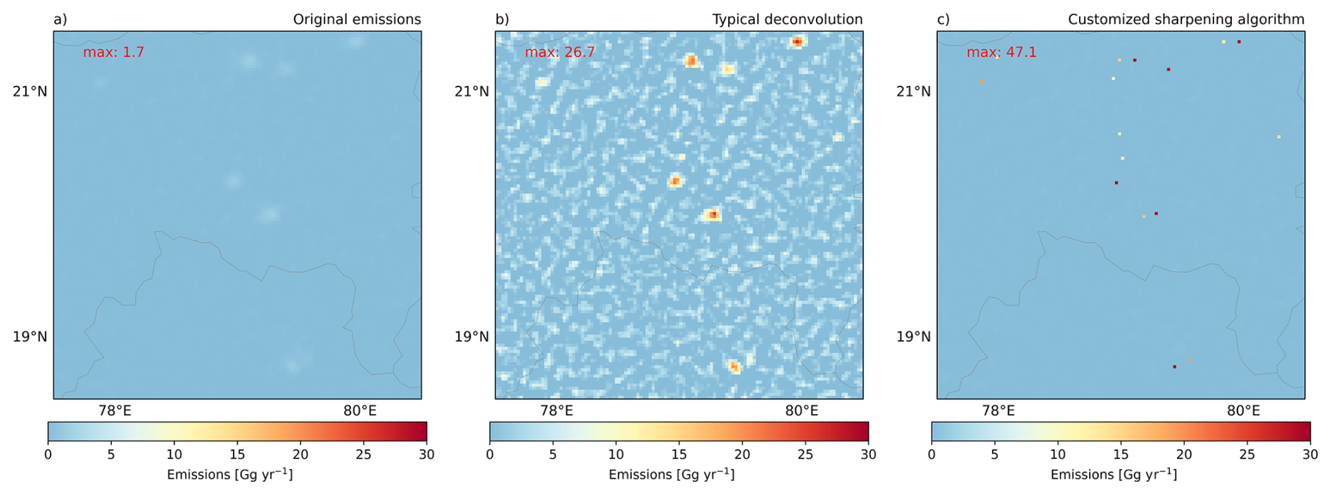
Figure 2 SO₂ emissions over a zoom-in region in India. (a) Original SO₂ emissions. (b) SO₂ emissions after the typical deconvolution. (c) SO₂ emissions after customized sharpening algorithm (sharpening applied in descending order of emission) (The same figure with a color bar starting from a negative value is shown in Fig. S3)

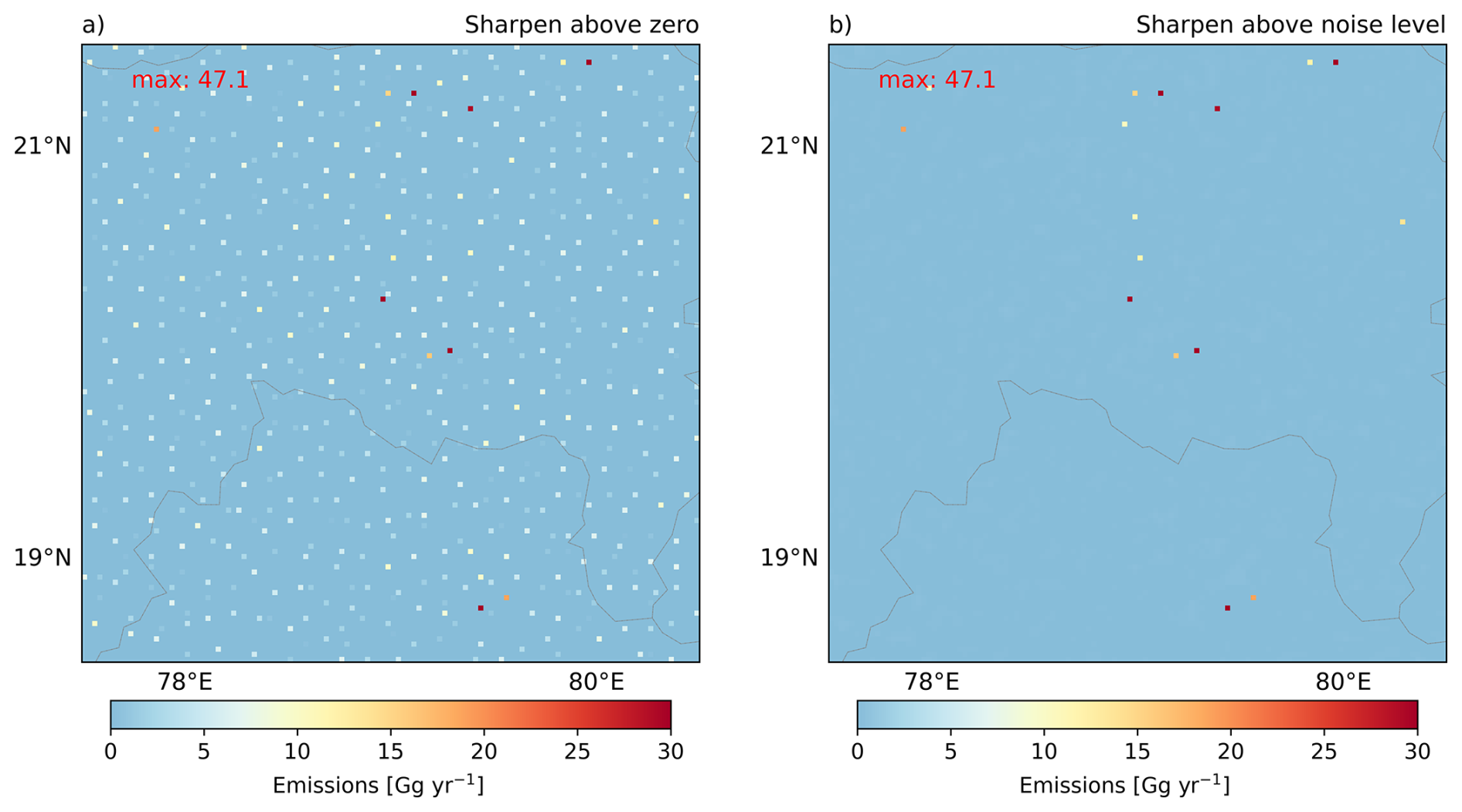
Figure 3 SO₂ emissions of a zoom-in region in India. (a) SO₂ emissions sharpened down to all non-zero values. (b) SO₂ emissions sharpened only above the noise level.

3.3 Sharpening algorithm

The sharpening kernel A is derived from the spreading kernel B. When requiring local mass balance, the sharpening kernel A used to reconstruct each point source emissions can be expressed by:

$$\begin{array}{}\text{(2)}& \mathbf{A}=I+\left(\mathbf{I}-\mathbf{B}\right)b_{\mathrm{00}}^{-\mathrm{1}},\end{array}$$

where b₀₀ is the central element of the kernel B, and I is the identity kernel. We cannot apply this sharpening kernel to the whole map Y because this would also sharpen spread emissions and increase the noise. Therefore, we define the following “local” sharpening kernel A^′

$$\begin{array}{}\text{(3)}& {\mathbf{A}}^{\prime }=\left\{\begin{array}{ll}\mathbf{A}& \text{at}(i,j)\\ \mathbf{I}& \text{elsewhere}\end{array}\right.\end{array}$$

In each iteration n, we select the location (i,j) with the highest remaining emission in emission map Y_n−1, which has not been selected in previous iterations. The updated emission map is then computed as:

$$\begin{array}{}\text{(4)}& {\mathbf{Y}}_{\mathbf{n}}={\mathbf{A}}^{\prime }\times {\mathbf{Y}}_{\mathbf{n}-\mathbf{1}}.\end{array}$$

Note that in typical deconvolution method, the sharpening kernel is applied to the entire region at once. However, sharpening in this way causes the point source emissions to add more noise as shown in Fig. 2b. We therefore use Eq. (4) to sharpen locations stepwise by using the local sharpening kernel of Eq. (3) for locations in a descending order of emission strength (from high to low), minimizing the risk of applying sharpening to regions dominated by the spread emissions or noise. There is total mass balance in each local area where sharpening is applied.

The step-wise process stops when the highest unsharpened value ${\mathbf{Y}}_{\mathbf{n}-\mathbf{1}}(i,j)$ is below the noise level in Y. This means we only sharpen emissions above the noise level (see noise level information in Sect. S6). This approach helps focusing on real point source emissions. If values below the noise level are sharpened, it will amplify the noise, making it harder to distinguish real point source from the sharpened noise. Figure 3 compares the results of sharpening emissions above zero and above noise level. In Fig. 3a, where all above zero grids are sharpened, the noise is also amplified.

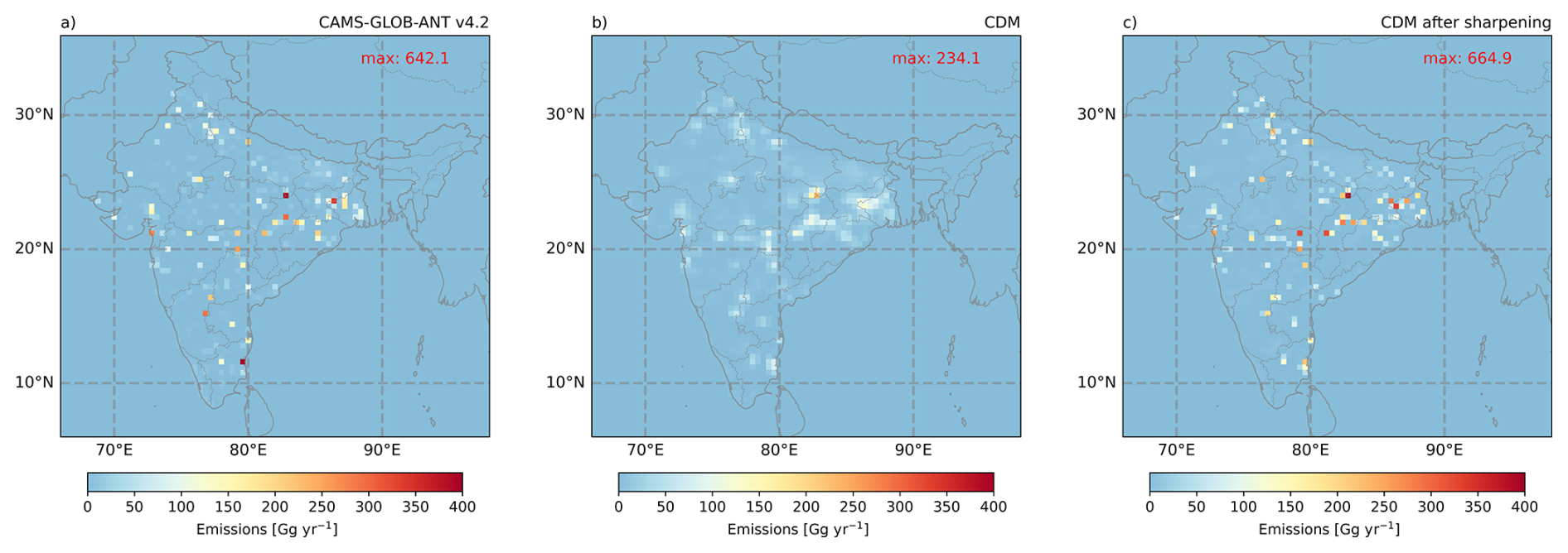
Figure 4 SO₂ emissions distribution averaged within December 2019 and November 2020. (a) CAMS emission inventory (CAMS-GLOB-ANT v4.2, interpolated to 0.4° × 0.4°). (b) SO₂ emissions calculated through classic divergence method (CDM). (c) Divergence method after sharpening using a 5 × 5 kernel.

4 Results and discussions

4.1 Model-based validation

Previous studies have shown the effectiveness of the divergence method in estimating emissions. We expect a further improvement combining the divergence method with our sharpening algorithm. To evaluate the performance of the combined approach, we implement it within a closed-loop validation process. Specifically, we apply the divergence method together with the algorithm to derive SO₂ emissions based on simulation results from the CAMS model, including SO₂ column densities, OH concentrations and IFS model-output wind fields. Since the input emissions used to drive the CAMS model is known, we can assess the accuracy of our method by comparing the derived top-down emissions with the original model input. Here we use as input the emission inventory CAMS Global Anthropogenic Emissions Inventory Version 4.2 (CAMS-GLOB-ANT v4.2) (Soulie et al., 2023; Copernicus Atmosphere Monitoring Service (CAMS), 2020) with the original spatial resolution of 0.1° × 0.1°, and the corresponding CAMS composition forecasts driven by this inventory from December 2019 to November 2020 as output in this closed-loop validation. Figure 4 shows the comparison between the input SO₂ emissions and the derived SO₂ emissions. There is a noticeable difference in distribution between the model input emissions (Fig. 4a) and the emissions derived from the divergence method (CDM) (Fig. 4b). The latter emission map appears more dispersed, with the point source emissions spreading into adjacent grid cells. This spreading effect also leads to a lower emission peak at the point source location, for example, the maximum value is much lower in Fig. 4b than in Fig 4a. In contrast, the model input emissions in Fig. 4a are more concentrated, showing higher values at the point source locations. To reduce this discrepancy, we sharpen Fig. 4b with the model-based 5 × 5 sharpening kernel. The size and the shape of this kernel are derived from the spreading pattern (Fig. S4) of “blurry” emissions (Fig. 4b) using Eq. (2). The emissions after sharpening in Fig. 4c prove that the algorithm effectively improves the emission estimates. The total emissions shown in Fig. 4b and c are the same and comparable to Fig. 4a, but the point-source emissions in Fig. 4c are no longer spread. Additionally, Fig. 5 compares the SO₂ emissions of point sources for the different methods. As shown in Fig. 5a, a clear underestimation is shown for SO₂ emissions derived only with the divergence method. But the underestimation is efficiently reduced after applying the sharpening as seen in Fig. 5b. It is important to note that the CAMS model resolution is relatively coarse (0.4° × 0.4°). At this resolution, some individual emissions are not well recovered during sharpening, because the spreading regions of the 5 × 5 kernels can overlap with several nearby point sources. Applying this combined approach to real measurements with finer spatial resolution will lead to a better performance, which will be shown in the following sections.

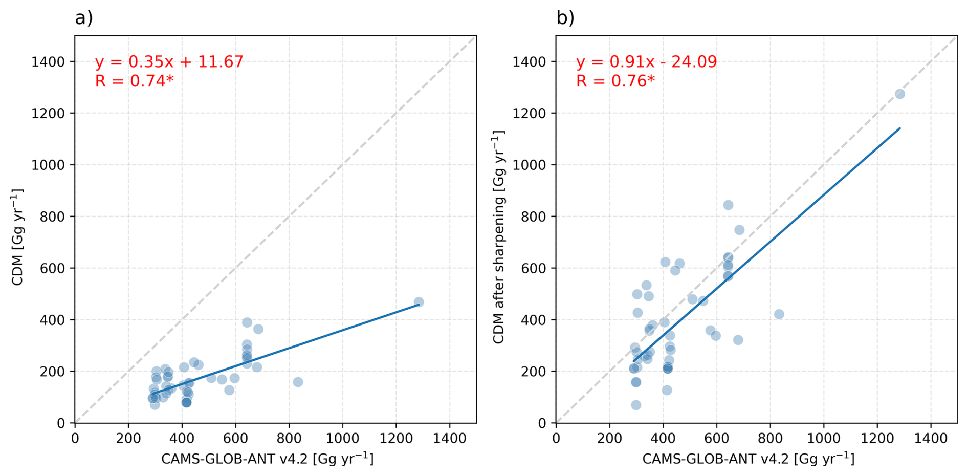
Figure 5 Comparison of SO₂ point source emissions between model input inventory (CAMS-GLOB-ANT v4.2, x axis) and model-based top-down estimate (y axis). The largest 50-point source emissions in CAMS-GLOB-ANT v4.2 are used in this comparison. (a) y axis represents the top-down emissions derived from classic divergence method (CDM). (b) y axis represents the top-down emissions from CDM sharpened by the 5 × 5 kernel. Since the top-down emission signal may be spatially shifted, the sum of emissions from two grid cells is used for comparison: one corresponding to the point source location and the other to the grid cell with the maximum emissions in the surrounding area.

4.2 Emission and distribution improvements on point sources

After the model-based evaluation, we apply the sharpening algorithm to satellite-based top-down SO₂ emissions at a resolution of 0.025° × 0.025°. At this high resolution, the emission signals of point sources are not easily visible on the large map over India. To better illustrate the improvement, we use all Indian coal power plants with annual power generation larger than 1500 MW and check their emission distribution at surrounding areas (9 × 9 grid cell areas) before and after sharpening. In total, 38 such power plants (Table S2) are included, and all of them are detected in our 1-year emission result (from December 2022 to November 2023). We average the emission distributions centered on these 38 point sources for each surrounding grid cell, with the results shown in Fig. S5. We see that the actual emission distribution before sharpening closely follows a 2D Gaussian pattern (Fig. S5a). This supports the Gaussian-shaped spreading pattern derived earlier from Fig. 1b. After sharpening the emission spread is removed and the point source emissions are enhanced by up to 28 times compared to the unsharpened case, while ensuring mass conservation (Fig. S5b). The emission signal becomes more concentrated into a single grid cell, effectively increasing the emission resolution to match the grid cell resolution. In addition to this averaged analysis, we also check the emission distribution of several individual point sources. In Fig. 6, four examples are given to show the effect of the sharpening in individual cases, the left figure shows the original distribution and the right figure after sharpening for an area of 9 × 9 grid cells. In Fig. 6a, the emissions of two sources are mixed before sharpening, but they are clearly separated in Fig. 6b. In Fig. 6c–f, a strong signal appears at the main source location, while smaller sources nearby are also visible. The small point source in Fig. 6d is and are newly detected power plant in our inventory. In Fig. 6g and h, the point source emissions are lower than the large point sources, the emission distribution before sharpening shows less of the characteristics of a Gaussian shape, making it more difficult to identify. However, after applying the sharpening algorithm the emission source is clearly localized and quantified.

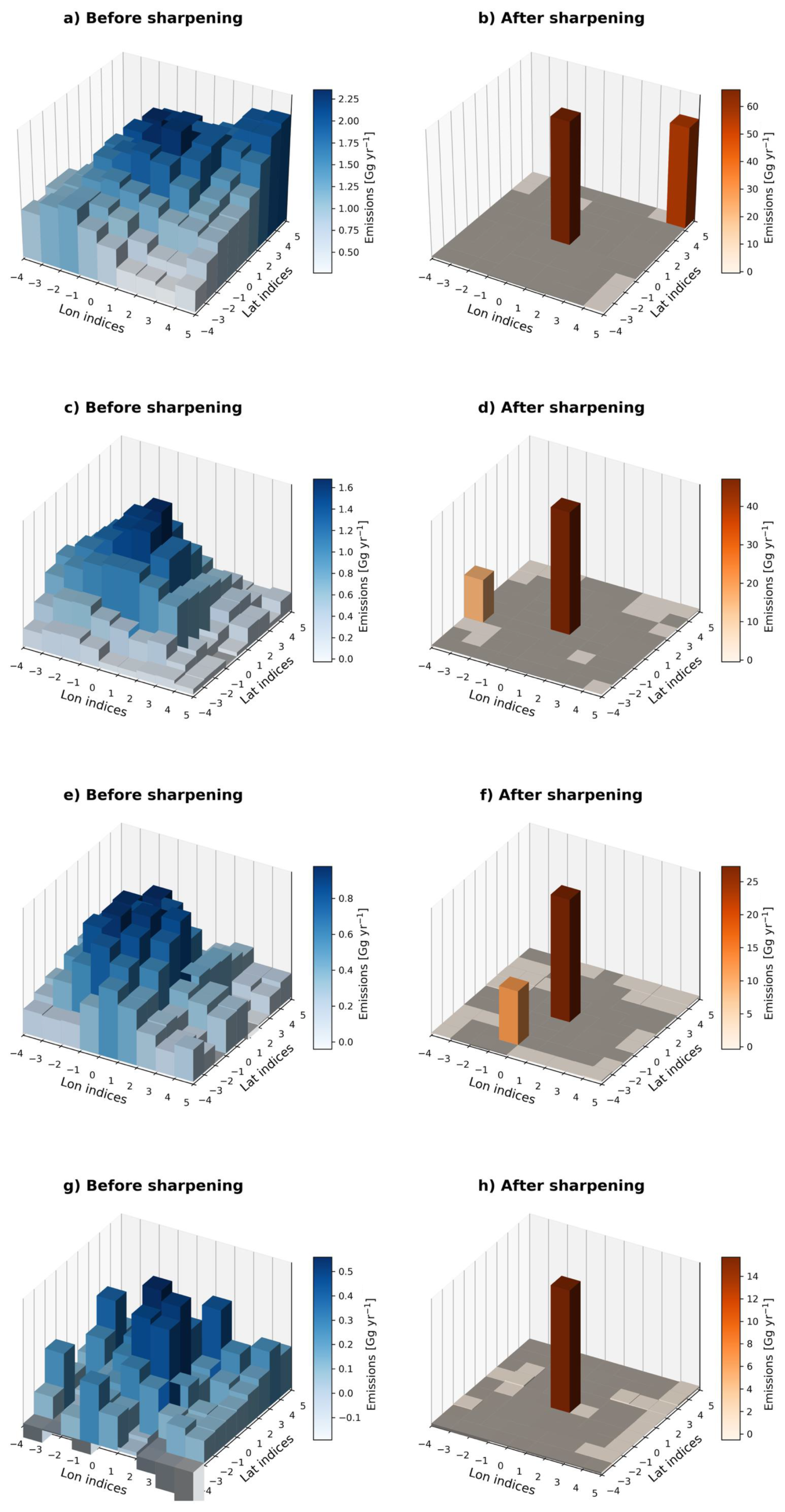
Figure 6 SO₂ annual emission distribution centered on a SO₂ point source within a 9 × 9 grid cell area. The left column represents the SO₂ emissions before sharpening and the right column represents the emissions after sharpening. (a, b) Vindhyachal Super Thermal Power Station (24.090° N, 82.675° E), with Renusagar Power Station (24.182° N, 82.793° E) located in the top-right corner of this 9 × 9 grid cell area. (c, d) Maharashtra State Power Station (20.012° N, 79.288° E) with the new detected Dhariwal Power Station nearby (20.009° N, 79.203° E). (e, f) Raichur Thermal Power Station (16.363° N, 77.363° E) with the Yermarus Thermal Power Station nearby (16.297° N, 77.355° E). (g, h) Unchahar Power Station (25.913° N, 81.338° E).

4.3 Location assessment

The improved emission resolution makes it easier to precisely locate the SO₂ point sources in the top-down emission inventory. To evaluate the location accuracy of the SO₂ point sources in our emission inventory, we compare the detected locations using one-year emission results (December 2022 to November 2023) with the actual locations of 82 known coal power plants with annual power generation larger than 1000 MW as shown in Fig. 7. The locations of the selected point sources are shown in Table S3. Among them, 51 power plants are detected within the same grid cell as their actual location, and 26 power plants are detected in the grid cells directly adjacent to the actual locations. If we consider the average TROPOMI pixel size (6.0 km × 6.0 km) as the resolution for detecting point sources, then 80 out of 82 power plants (approximately 97.5 %) are successfully located within this range using emissions derived from TROPOMI measurements. The remaining 2 power plants are detected two grid cells away from their actual locations, which is the result of the influence from nearby sources, e.g. other closely located point sources or large urban areas, may cause the peak VCD and resulting emissions shift away from the point source location.

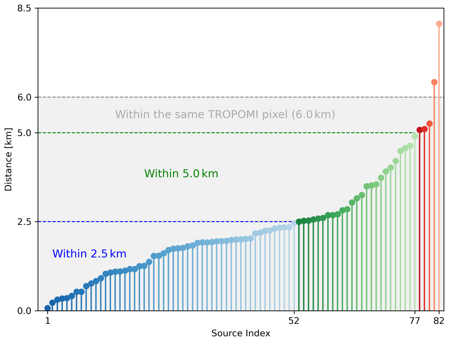
Figure 7 Distance between the actual and our detected locations of large Indian SO₂ point sources. The grid resolution of the emissions is 0.025° × 0.025° (approximately 2.5 km × 2.5 km per grid cell). Blue dots below 2.5 km: detected and actual locations fall within the same grid cell. Green dots between 2.5 and 5.0 km: Detected locations are in grid cells directly adjacent to the actual locations. Red dots above 5.0 km: detected locations are in grid cells that are one grid cell further away from the actual locations. Gray shadow below 6.0 km: detected and actual locations fall within the same TROPOMI pixel (on average 6.0 km × 6.0 km).

4.4 Point source detection ability

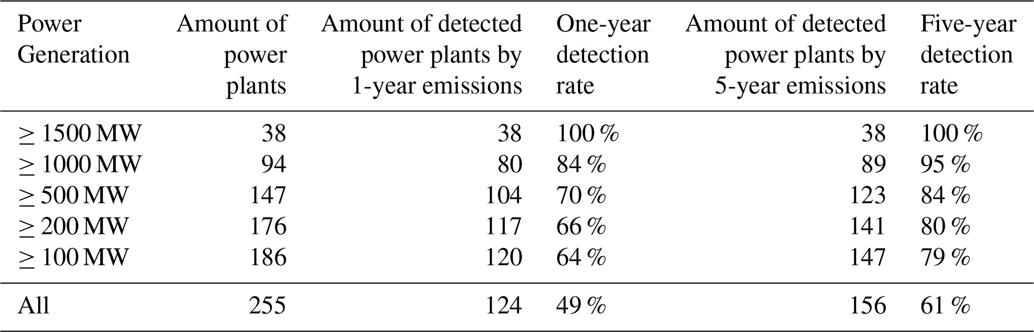
Since the point source emission signals have been enhanced, we expect more emission signals to be visible on our satellite-based emission map. Coal-based power plants are the largest sector for SO₂ emissions in India. To assess our results, we compare both annual and 5-year averaged emission signals with the actual locations of all coal-based power plants across the country. These plants have annual capacities ranging from 10 MW to 4760 MW. Because some sources may have low emissions in certain years and the emission peaks may not align exactly with plant locations, we define a power plant as “detected” if the annual emission signal above the annual detection threshold 10 Gg yr⁻¹ or the 5-year averaged emission signal above the corresponded detection threshold 3.4 Gg yr⁻¹ within 6.0 km of the plant (see Sect. S6 for more details on noise levels and detection thresholds). As summarized in Table 1, long-term averaged emissions allow more power plants to be detected. All large power plants with annual power generation larger than 1500 MW are identified in both annual and 5-year results. In addition, approximately 80 % of power plants with capacities larger than 100 MW yr⁻¹ are successfully detected using 5-year averages, while the emissions of the remaining 20 % of power plants are lower than the noise level or 6.0 km further away from the actual location. These detected plants represent 99 % of India's total coal-based power generation. For large power plants with annual capacities above 1000 MW, contributing 77 % of the total generation, the detection rate reaches 95 %. The higher the output, the more coal is burned, making emissions more likely to be detected.

Table 1 Comparison between the India coal-combustion thermal power plants and point source emission signal in this study.

4.5 Newly detected point sources

We find some new operating SO₂ point sources using both annual and 5-year averaged SO₂ emission inventories. These emissions are absent in the Indian power plant database and are also not identified by the top-down SO₂ catalogue MSAQSO₂L4. These new point sources include not only coal-based power plants, but also cement factories, crude oil production facilities, a chemical fertilizer factory, and copper, steel, and aluminum industries. Table 2 provides the list and locations of these sources. Many newly detected sources are small and located close to known large point sources, but their weaker signals are distinguishable in our inventory. The annual emission inventory better distinguishes small point sources located near large ones, whereas the long-term averaged inventory provides more precise source locations. Most operating point sources show persistent SO₂ emission signal over five years. However, Rashtriya Chemicals Fertilizers (RCF) complex involving a sulfuric acid plant located in Trombay, Maharashtra is detected only for the year 2021. RCF reported that sulfur consumption in the financial year March 2021–March 2022 was 2.7 times higher than in 2020-2021 (https://www.rcfltd.com/public/storage/investers/1669721755.pdf, last access: 20 February 2026), indicating substantially higher potential SO₂ emissions in 2021. This indicates that applying the sharpening algorithm to short-term emission results enables the analysis of temporal variability, including emission changes and possible commissioning or shutdown events. In contrast, the Phil Coal Beneficiation and Sponge Iron Cluster is only detected in the 5-year averaged inventory, but not in any individual annual result. This is because long-term averaging results reduces noises, allowing the sharpening algorithm to better detect small but stable emitters.

Table 2 Newly detected SO₂ point sources in India.

5 Conclusion

In this study, we developed a sharpening algorithm to improve the resolution of SO₂ emissions estimated using the flux-divergence method and TROPOMI satellite data. Before applying the algorithm, emissions from point sources tend to spread, making it difficult to detect smaller sources or distinguish closely located sources. After applying the algorithm, the emission signals become sharper and more concentrated at their true locations. On average, annual emissions at point source locations increase by up to 28 times compared to before the sharpening at a resolution of 0.025° × 0.025°. This sharpening helps to separate emissions from nearby sources. To validate the results, we compared our results with the locations of 82 coal power plants. We find that 97.5 % of the detected sources fall within the same TROPOMI pixel as their real locations. We detected about 80 % of all coal power plants with power generation larger than 100 MW yr⁻¹, which account for 99 % of India's total coal-based electricity generation. With the improved signal, we also identified 22 new point sources not previously reported. These include coal-based power plants, but also cement factories, crude oil production facilities, a chemical fertilizer factory, and copper, steel, and aluminum industries. By comparing the annual and 5-year averaged emission results, we find that the annual emission inventory better distinguishes small point sources located near large ones, whereas the long-term averaged inventory provides more precise source locations. The sharpening algorithm can be applied on both short- and long-term average emissions to enhance the spatial resolution. Long-term averaging reduces emission noise, allowing smaller and stable point sources to be precisely identified, but it might miss small point sources that appear only over short time periods. Short-term emission maps enable analysis of temporal changes, such as the emission variation of the identified sources, or even the commissioning of new facilities or shutdowns. At very fine temporal resolution (e.g. monthly), noise dominates, and fewer point sources can be reliably identified. Once the noise level is determined, the application of the sharpening algorithm separates the noise and the emission signals. If a point source is located near the edge or corner of a grid cell, the emission signal may be shifted to an adjacent grid cell. So, to estimate actual emissions, we still recommend summing emissions over a small area around the point source. Although this algorithm is developed for SO₂, it can also be applied to other short-lifetime pollutants emitted by point sources like NO_x. It helps sharpen emission signals on existing grid cells and is a useful step toward building accurate emission inventories. For long-living species having a strong background concentration, like CH₄, we have not done any tests yet.