Quantifying CH₄ point source emissions with airborne remote sensing: first results from AVIRIS-4

Atmospheric concentration of methane (CH₄), a potent greenhouse gas, increased significantly since pre-industrial times, with anthropogenic emissions originating primarily from agriculture, fossil fuel sector and waste management. However, considerable uncertainties persist in the detection and quantification of anthropogenic CH₄ emissions. In this study, we present first CH₄ observations, plume detections and emission estimates from the new state-of-the-art Airborne Visible InfraRed Imaging Spectrometer 4 (AVIRIS-4), which participated in a blind controlled release experiment in September 2024 in southern France. We used an albedo-corrected matched filter to retrieve CH₄ maps from the spectral images and estimated CH₄ emission with the Integrated Mass Enhancement (IME) and Cross-Sectional Flux (CSF) methods. Our results demonstrate that AVIRIS-4 can reliably detect emissions as low as 5.5 kg CH₄ h⁻¹ under good weather conditions at low flight altitudes (< 1500 m) and 1.45 kg CH₄ h⁻¹ under ideal conditions. These low-altitude detection limits are substantially lower than published detection limits for the predecessor instrument AVIRIS-NG, which were in the order of 10–16 kg CH₄ h⁻¹ under comparable conditions. While AVIRIS-4 provides highly accurate CH₄ maps at < 0.5 m resolution, emission estimation is limited by the accuracy of the effective wind speed, whose uncertainty and natural variability contribute substantially to the overall uncertainty. Using wind speed at source height performs well for small releases (below 20 kg CH₄ h⁻¹) (rRMSE =1.065; rMBE =0.361) and overall (rRMSE =0.702; rMBE =−0.204). Using literature-derived effective wind speeds improves the apparent fit between estimated and reported CH₄ emissions, but degrades performance both in overall agreement (rRMSE =2.098; rMBE =0.964) and for low-emission events (rRMSE =2.367; rMBE =1.711). Interestingly, the high spatial resolution makes it possible to retrieve the cast shadow of the CH₄ plume, which can be used to estimate source and plume height, and could provide an approach for better constraining the height-dependency of the effective wind speed. On the bottom line, the controlled release experiment provides critical insights into the sensor's capabilities and guides further improvements to detect and quantify low intensity sources in the fossil fuel and waste management sectors, with implications for more accurate global greenhouse gas monitoring.

1 Introduction

Methane (CH₄), a potent greenhouse gas with a global warming potential 28 times higher than CO₂ on a timescale of 100 years, has seen an almost threefold rise from 700 ppb pre-industrial levels to over 1900 ppb due to natural and anthropogenic sources (Seinfeld and Pandis, 2016). Major contributors include agriculture, fossil fuels, and waste. Due to its short lifetime of only 9 years, CH₄ is removed more quickly compared to most other greenhouse gases. Reducing CH₄ emissions is therefore considered an effective measure to mitigate anthropogenic climate change in the near term. However, there are still significant uncertainties in the quantification of anthropogenic CH₄ emissions (Saunois et al., 2020).

For instance, Saunois et al. (2020) estimated that uncertainties in emissions from the fossil fuel sector are around 20 %–35 % with strong regional variations. Reducing these uncertainties is challenging for several reasons. One of them is the fact that an important fraction of anthropogenic CH₄ emissions, e.g., from the fossil fuel sector, result from unintentional leakage, which cannot be accurately quantified. Additionally, global CH₄ emission estimates depend on a network of monitoring stations, which is dense and accurate in northern and mid-latitudes but sparser in other regions (Saunois et al., 2020). For these reasons, satellite remote sensing observations of CH₄ have been used to estimate the emissions in a top-down approach (e.g. Alexe et al., 2015; Bousquet et al., 2018; Fraser et al., 2013). These remote sensors can be separated into area flux mappers (e.g. Sentinel-5P, MethaneSAT and GOSAT-GW) which are designed to have a global to regional coverage and point flux mappers (e.g. Landsat-8, Sentinel-2, GHGSat, PRISMA and EnMAP) which are used to observe regional to local emissions (Jacob et al., 2022).

Most of the currently available CH₄ imagers are limited by spatial and/or spectral resolution which hinders the precision and accuracy of the emission estimates (Bousquet et al., 2018). This results in high detection limits in the range of a few 100 to several 1000 kg CH₄ h⁻¹ for spaceborne instruments such as Sentinel-2 and Sentinel-5, PRISMA, EnMAP or GHGSat (e.g. Jacob et al., 2022; Gorroño et al., 2023; Joyce et al., 2023). For airborne instruments with a higher spatial resolution such as MethaneAIR, GHGSat-AV and the Airborne Visible InfraRed Imaging Spectrometer – Next Generation (AVIRIS-NG), the detection limit decreases to 10 to 100 kg CH₄ h⁻¹ under favourable conditions (e.g. Cusworth et al., 2021; Duren et al., 2019; Jongaramrungruang et al., 2022; Kuhlmann et al., 2025; Guanter et al., 2025).

CH₄ emissions from sources with small emission strengths that cannot be quantified from space (< 100 kg CH₄ h⁻¹) are crucial for two reasons: First, leakages from the production and use of fossil fuels are often small and remain undetected by satellite-based approaches. Second, CH₄ emissions from oil and gas production have a lognormal distribution with many small sources but only a few large ones (e.g. Balcombe et al., 2018; Stavropoulou et al., 2023; Williams et al., 2025). Accurate knowledge of the emission distribution of sources from a given sector or country is crucial for extrapolating CH₄ emissions from the entire sector or country by accounting for sources below the detection limit (Zavala-Araiza et al., 2015; Zhang et al., 2023; Kuhlmann et al., 2025).

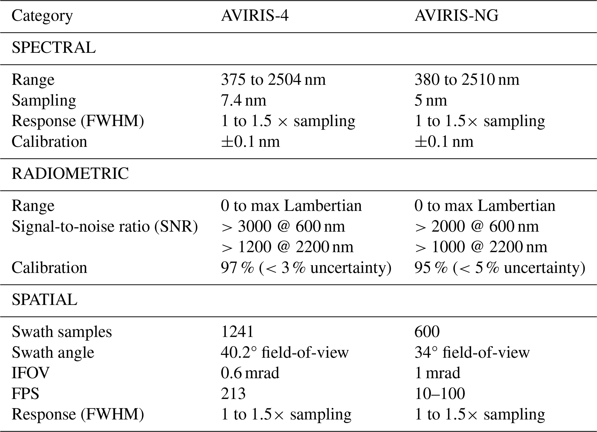
The detection of low intensity CH₄ sources requires a sensor that combines high spatial resolution with a good signal-to-noise ratio. One such state-of-the-art sensor is the new Airborne Visible InfraRed Imaging Spectrometer 4 (AVIRIS-4). It was developed by NASA JPL as a successor of AVIRIS-NG in parallel to its sister instruments Earth Surface Mineral Dust Source Investigation (EMIT) and AVIRIS-3 which are in service on board the ISS and as airborne sensor respectively (Hueni et al., 2025). In comparison with its predecessor, AVIRIS-4 has traded some of its spectral resolution in order to enhance its spatial resolution and SNR (see Table 1). In this paper, we present the processing chain for retrieving CH₄ emissions from AVIRIS-4 measurements, show CH₄ maps and emission estimates from a blind controlled release experiment and characterise the capabilities and limitations of AVIRIS-4 for CH₄ emission quantification. The analysis considers the influence of flight altitude, meteorological conditions such as wind speeds and atmospheric stability, illumination and viewing conditions, and surface reflectance on the detection limit and the quality of the emission quantifications, providing guidance for future campaigns.

2 Data and Methods

This section covers the description of AVIRIS-4 (Sect. 2.1) used for the acquisition of remote sensing data in the controlled release experiment (Sect. 2.2) and the data processing chain from radiance data processing (Sect. 2.3), CH₄ retrieval (Sect. 2.4) and CH₄ emission estimation (Secti. 2.5) to the estimation of uncertainties (Sect. 2.6).

2.1 AVIRIS-4 sensor specification

AVIRIS-4 is a state-of-the-art imaging spectrometer with identical core components as NASA JPL's AVIRIS-3 and the EMIT spectrometer (Green et al., 2022; Shaw et al., 2022; Hueni et al., 2025). The spectrometer is equipped with a 1280-pixel sensor array and records hyperspectral data in 328 bands spanning the ultraviolet (UV) to the shortwave infrared (SWIR). In practice, 1241 pixels receive sufficient illumination and SNR, and 287 bands are retained for data processing. Detailed sensor specifications are provided in Hueni et al. (2025). Compared to its predecessor it offers enhanced stability, spatial sampling interval (hereafter referred to as spatial resolution) and signal-to-noise ratio (SNR) (see Table 1).

Table 1 Specifications of AVIRIS-4 compared to AVIRIS-NG, adapted from Green et al. (2022) and Hueni et al. (2025).

2.2 Controlled release experiment

The data for this analysis was acquired during a single-blind controlled release experiment organised by the Environmental Assessment and Optimization Group at Stanford University between the 16 and 20 September 2024 at the TotalEnergies Anomalies Detection Initiatives (TADI) site in Lacq in the south of France (latitude: 43.412°, longitude: −0.636°, elevation a.m.s.l.: 95 m) (see Fig. 1a). A total of 13 commercial and academic teams, using a range of technologies – including continuous monitoring, vehicle-based measurements, drones, airborne in-situ measurements, remote sensing from aircraft, and satellites – participated in the experiment. The results of all teams were collected and analysed in McManemin (2025). On each campaign day (08:00–18:00 CEST), up to 9 individual controlled releases with rates varying between 0.02 and 350 kg CH₄ h⁻¹ were conducted at different unknown heights between 0.01 to 6.5 m above ground and at different unknown locations on the study site (see Fig. 1b). Each release lasted for 45 min and was followed by a 15 min break before the start of the next release. In some periods, no CH₄ was released to enable the detection of false positives. Additionally, the wind speed was measured using a ZX 300 Doppler wind lidar positioned 100 m from the emission sources. The instrument recorded horizontal and vertical wind speeds, as well as wind direction, at preselected heights between 10 and 300 m above ground level, with a temporal resolution of approximately 20 s. Participating teams were aware of the timing of releases while locations and flow rates of the releases as well as the wind data were only made available after all teams had submitted their initial emission estimates. Details of the release experiment, the participating teams and the synthesis can be found in McManemin (2025). For the campaign, AVIRIS-4 was mounted on a hydraulic stabilisation mount and built into a Cessna 208B Grand Caravan EX. The aircraft flew over the release site in either north-south or east-west direction at different altitudes of 12 000, 9000, 6000, 4200 and 3300 ft or 3660, 2740, 1830, 1280, 1000 m above mean sea level (a.m.s.l.) (see Fig. 1a). This resulted in average spatial resolutions of 2.0, 1.5, 1.0, 0.7 and 0.5 m across-track and 0.35 m along-track. For the remainder of the article, all wind speed heights are given in metres above ground level and all flight altitudes in feet a.m.s.l.

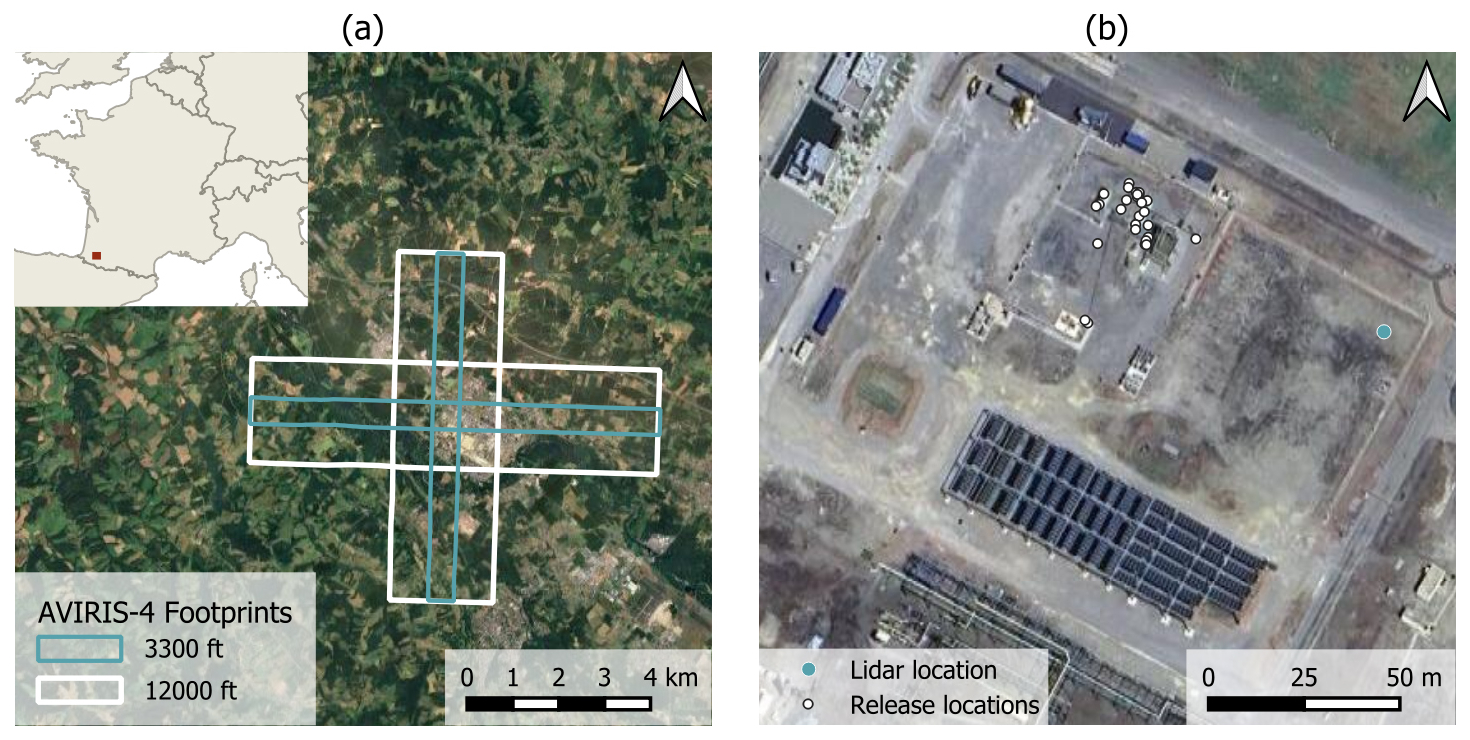
Figure 1 (a) Location of the controlled release experiment at the TADI site in the south of France (red polygon in the inset map). Superimposed are the imaging footprints of AVIRIS-4 for overpasses at 3300 and 12 000 ft. (b) Aerial view of the site with the locations of the wind lidar as well as the potential release locations. Imagery: © 2025 Airbus, CNES, Landsat, Copernicus, Maxar Technologies, map data: © 2025 Google.

2.3 Data processing

2.3.1 Radiometric and spectral calibration, georeferencing

The level 0 data acquired by AVIRIS-4 consists of raw digital numbers organized into along-track and across-track spatial dimensions and a spectral dimension. The level 0 data was converted into level 1 at-sensor radiances (in $\mathrm{\mu }\mathrm{W}{\mathrm{cm}}^{-\mathrm{2}}{\mathrm{nm}}^{-\mathrm{1}}{\mathrm{sr}}^{-\mathrm{1}}$) using laboratory-measured calibration coefficients. The level 1 data was georeferenced using a parametric approach (Schläpfer and Richter, 2002), where the geometry of the sensor, its location and orientation acquired from global navigation satellite system (GNSS) and inertial navigation system (INS) data were combined with a digital elevation model (IGN, 2018) to project the radiometrically corrected data onto the surface with sub-pixel accuracy. Details on the processing are described in Hueni et al. (2025).

2.3.2 Masking of shadows and water surfaces

Observations over dark surfaces such as cast shadows and water bodies have a low SNR and therefore produce artefacts when processing the data. Additionally, cast shadows only contain diffuse radiance, which is inconsistent with the non-scattering assumption in CH₄ retrieval. Cast shadows were especially pronounced in our data, as the controlled release experiment took place in late September under low solar zenith angles (SZA). For this reason, we masked these areas using a modified version of the cast detection method described in Schläpfer et al. (2018), using radiances at 450 nm for blue (L_b), 670 nm for red (L_r) and 780 nm for near-infrared (NIR) (L_n):

$$\begin{array}{}\text{(1)}& i_{sh}={\displaystyle \frac{L_{\mathrm{r}}+k_n(L_{\mathrm{n}}-L_{\mathrm{r}}{)}_{>\mathrm{0}}}{L_{\mathrm{b}}}}\cdot {\displaystyle \frac{\mathrm{1}}{a{e}^{b{L}_{\mathrm{b},\mathrm{dark}}}}}.\end{array}$$

We used the default parameters k_n=0.1, a=1.58 and $b=-\mathrm{0.04}$ from Schläpfer et al. (2018). Next, we divided the inverse of the resulting index by the integrated radiance over all wavelengths. After empirical evaluation, values larger than 0.25 were masked prior to applying the matched filter.

2.4 CH₄ retrieval

We retrieved CH₄ maps from the AVIRIS-4 radiance cubes using the computationally efficient matched filter approach following Foote et al. (2020) and further refined by Kuhlmann et al. (2025). The filter detects a known signal within a noisy background by enhancing the signal relative to the noise, effectively maximising the output signal-to-noise ratio under the assumption of additive Gaussian noise.

2.4.1 Matched filter

Using a linearised form of the Beer-Lambert law, the matched filter (MF) takes the form

$$\begin{array}{}\text{(2)}& {\mathit{\alpha }}_{\mathit{ϵ}}={\displaystyle \frac{({\mathit{L}}_{\mathrm{obs}}-\widehat{\mathit{\mu }})\cdot {\widehat{\mathbf{S}}}^{-\mathrm{1}}\cdot \mathit{t}}{{\mathit{t}}^{\top }\cdot {\widehat{\mathbf{S}}}^{-\mathrm{1}}\cdot \mathit{t}}}\end{array}$$

where α_ϵ represents the CH₄ column enhancement, L_obs the observed spectrum in the two wavelength ranges 1480 to 1800 and 2080 to 2500 nm, $\widehat{\mathit{\mu }}$ and $\widehat{\mathbf{S}}$ the median and covariance of the observed spectrum and $\mathit{t}=\widehat{\mathit{\mu }}\cdot -\mathit{s}$ the target spectrum. We used the negative of the unit absorption spectrum of CH₄ s to align Eq. (2) with derivations in other studies. Thereby, s is calculated using the radiative transfer equation assuming a geometric air mass factor (AMF), no atmospheric scattering according to Kuhlmann et al. (2025) and a CH₄ enhancement ϵ in the lowest 1000 m layer respectively. The calculation of the plume-specific enhancement was achieved through an iterative approach, wherein the CH₄ maps were initially derived under the assumption of an enhancement of 0.01 ppm. The mean enhancement in the detected plume was then used for the subsequent iteration of the matched filter, which converged after three iterations with changes between successive iterations falling below a 5 % threshold. Our iterative approach reduces the approximation error introduced by the linearisation of the Beer-Lambert law by expanding around the current estimate of α rather than α=0, which decreases the linearisation error quadratically in the update step. For large enhancements, this substantially mitigates non-linear absorption effects. The mathematical derivation can be found in the Supplement.

2.4.2 Lognormal matched filter

Due to the linearisation of the Beer-Lambert law used in the derivation of most matched filter approaches, they are only valid for weak CH₄ enhancements. Therefore, Schaum (2021) argued that a lognormal matched filter (LMF) provides the uniform most powerful solution for the detection of trace gas plumes, which takes the following form:

$$\begin{array}{}\text{(3)}& {\mathit{\alpha }}_{\mathit{ϵ}}={\displaystyle \frac{\left(\ln \right({\mathit{L}}_{\mathrm{obs}})-\widehat{\mathit{\mu }})\cdot {\widehat{\mathbf{S}}}^{-\mathrm{1}}\cdot \mathit{s}}{{\mathit{s}}^{\top }\cdot {\widehat{\mathbf{S}}}^{-\mathrm{1}}\cdot \mathit{s}}}\end{array}$$

where s is the same unit absorption spectrum as above. This approach has been implemented and evaluated by Pei et al. (2023) for synthetic WRF-LES and observed data from the PRISMA satellite. According to Schaum (2021), the LMF could improve the detection performance for pixels with attenuated signal, e.g. with weak enhancement or at higher flight altitudes, due to the more realistic mean spectrum $\widehat{\mathit{\mu }}$ in logarithmic space. In the present study, we evaluated the LMF only exploratively to illustrate its behaviour on AVIRIS-4 data with an emphasis on the smallest and largest release events.

2.4.3 Albedo correction

We applied the matched filter to the at-sensor radiance of each across-track position to avoid striping caused by differences in radiometric and spectral calibration of the sensor pixels. However, as outlined in Fahlen et al. (2024), the assumption that the reference solar spectrum L₀ can be approximated by the mean spectrum $\widehat{\mathit{\mu }}$ introduces a bias in the CH₄ column enhancement α_ϵ over heterogeneous surfaces, which must be corrected as follows:

$$\begin{array}{}\text{(4)}& {\mathit{\alpha }}_{\mathrm{corr}}={\displaystyle \frac{\mathrm{1}}{R}}\times {\mathit{\alpha }}_{\mathit{ϵ}}\mathrm{with}R={\displaystyle \frac{({\mathit{L}}_{\mathrm{obs}}\times -\mathit{s})\cdot {\widehat{\mathbf{S}}}^{-\mathrm{1}}\cdot \mathit{t}}{{\mathit{t}}^{\top }\cdot {\widehat{\mathbf{S}}}^{-\mathrm{1}}\cdot \mathit{t}}}\end{array}$$

While the correction factor helps mitigate biases in CH₄ enhancements, it also amplifies retrieval noise for dark surfaces with a low signal-to-noise ratio. This effect could be mitigated by masking cast shadows and water surfaces before applying the matched filter.

2.4.4 Plume shadow correction

In some of the AVIRIS-4 observations, we observed double plumes due to plume shadows (see Sect. 3.5.4). They present a challenge for emission estimation because the CH₄ retrieval assumes that the light traverses the plume twice, assuming a geometric AMF that depends both on the solar zenith angle (SZA) and viewing zenith angle (VZA):

$$\begin{array}{}\text{(5)}& {\mathrm{AMF}}_{\mathrm{geom}}=\sec \left(\mathrm{SZA}\right)+\sec \left(\mathrm{VZA}\right)\end{array}$$

At the source location, however, the signal originating from the plume does not pass through the plume a second time after ground reflection, and thus it is independent of the VZA. Consequently, CH₄ enhancements should be scaled by c_plume:

$$\begin{array}{}\text{(6)}& c_{\mathrm{plume}}={\displaystyle \frac{{\mathrm{AMF}}_{\mathrm{geom}}}{\sec \left(\mathrm{VZA}\right)}}\end{array}$$

For the plume shadow enhancement, the respective correction factor is given by

$$\begin{array}{}\text{(7)}& c_{\mathrm{shadow}}={\displaystyle \frac{{\mathrm{AMF}}_{\mathrm{geom}}}{\sec \left(\mathrm{SZA}\right)}}\end{array}$$

When the plume and its shadow were clearly resolved, we estimated the emissions and applied the corresponding correction factor. However, when the plumes partially overlapped, this separation was not feasible, limiting the applicability of the correction method. In such situations, we employed the integrated mass enhancement (IME), which aggregates all detected pixels without explicitly distinguishing between the plume and its shadow.

2.5 CH₄ emission estimation

To estimate the CH₄ emissions, we used the integrated mass enhancement (IME) and cross-sectional flux (CSF) method implemented in the Python library for data-driven emission quantification (ddeq) (Kuhlmann et al., 2024). We used the CSF for longer plumes and more turbulent conditions as it averages the fluxes along several cross-sections. Conversely, the IME was used for short plumes and plumes that deviate from a Gaussian plume shape such as for overlapping double plumes. Both methods assume steady-state conditions of wind speed and emission rate. Limits of this assumption are further discussed in Sect. 4.2.

All mass-balance based methods require an estimate of the wind speed U. Ideally, U would correspond to the effective wind speed U_eff, which is the mean speed at which the plume is transported (Kuhlmann et al., 2024). However, as the vertical CH₄ profile is unknown, we used four different approaches to obtain a wind speed estimate:

1. 10 m wind speeds U₁₀ from ERA5 reanalysis data (Hersbach et al., 2018) as used for the initial reporting in McManemin (2025) as ground-based lidar measurements were not available prior to unblinding.

2. 10 m wind speeds U₁₀ from wind lidar measurements.

3. A linear scaling of the 10 m wind speed derived from model simulations for GHGSat (Varon et al., 2018):

   $$\begin{array}{}\text{(8)}& U_{\mathrm{eff}}=\mathrm{1.47}\cdot U_{\mathrm{10}}\end{array}$$

4. Wind speed at source height U_s, assuming a logarithmic wind profile (Fleagle and Businger, 1980; Seinfeld and Pandis, 2016). Wind profiles were derived assuming a surface roughness of 0.1 m and using on-site measurements of temperature and wind speed, combined with sensible heat fluxes from ERA5 reanalysis data (Hersbach et al., 2018). While plume rise and vertical mixing were not explicitly incorporated into the wind speed calculations, their potential influence was accounted for in the uncertainty analysis.

We also conducted a sensitivity analysis using lidar wind speeds at other elevations above ground level.

2.5.1 Integrated mass enhancement

The IME approach derives the emission rate Q based on the integrated mass enhancement M of a plume and a residence time τ during which CH₄ resides within the detectable plume. This residence time is approximated by the wind speed U and the length L of the detectable plume (Kuhlmann et al., 2024).

$$\begin{array}{}\text{(9)}& Q=\mathit{\tau }\cdot M={\displaystyle \frac{U}{L}}\cdot M\end{array}$$

The plume length L was calculated as the arc length of the centre line curve fitted to the detected plume.

The integrated mass M was computed as

$$\begin{array}{}\text{(10)}& M=\sum _{(i,j)\in {\mathcal{P}}_{\mathrm{a}}}^n(V_{i,j}-V_{\mathrm{bg}})\cdot A_{i,j}\end{array}$$

where V_i,j is the vertical column density, V_bg is the background vertical column density, and A_i,j is the pixel area. The trace gas mass was summed up over the n pixels of the integration area 𝒫_a which was obtained by a sufficient extension of the detected plume in the crosswind direction to include pixels with enhancements below the detection limit. A local CH₄ background V_bg was calculated by applying a low-pass Gaussian filter to the CH₄ maps after masking the enhancements including a buffer (Kuhlmann et al., 2024).

2.5.2 Cross-sectional flux method

For the CSF, the detected plume is divided into multiple polygons. As in Kuhlmann et al. (2024), a Gaussian curve with linear background trend was then fitted to the CH₄ enhancements of each polygon to obtain the line densities q:

$$\begin{array}{}\text{(11)}& g\left(y\right)={\displaystyle \frac{q}{\sqrt{\mathrm{2}\mathit{\pi }}\mathit{\sigma }}}\exp \left(-{\displaystyle \frac{(y-\mathit{\mu }{)}^{\mathrm{2}}}{\mathrm{2}{\mathit{\sigma }}^{\mathrm{2}}}}\right)+my+b\end{array}$$

here, y is the across-plume direction, σ to the standard width and μ to the mean of the fitted Gaussian curve with linearly changing background with slope m and offset b.

The emissions Q were then calculated as the product of the wind speed U and the uncertainty-weighted mean of all line densities $\stackrel{\mathrm{‾}}{q}$:

$$\begin{array}{}\text{(12)}& Q=U\cdot \stackrel{\mathrm{‾}}{q}\end{array}$$

2.6 Estimation of uncertainty

Below we describe how uncertainty components are estimated and propagated for each input to the emission quantification.

2.6.1 CH₄ Columns

The uncertainty of CH₄ columns σ_V was calculated as

$$\begin{array}{}\text{(13)}& {\mathit{\sigma }}_V=\sqrt{{\mathit{\sigma }}_t^{\mathrm{2}}+{\mathit{\sigma }}_{{\mathrm{CH}}_{\mathrm{4}}}^{\mathrm{2}}}\end{array}$$

where ${\mathit{\sigma }}_{{\mathrm{CH}}_{\mathrm{4}}}$ is the standard deviation of retrieved CH₄ columns in a plume-free region next to the release location with similar surface properties. σ_t represents correlated uncertainties in the target t due to no-scatter assumptions for the calculation of the unit absorption spectrum s, which was estimated at a conservative 5 % for this campaign based on Kuhlmann et al. (2025).

2.6.2 Pixel area

Uncertainty in pixel area (σ_A) is treated as a systematic spatial uncertainty, reflecting geolocation and georectification errors. During this campaign, geolocation accuracy was reduced due to a faulty cable, which impaired the temporal synchronization between GNSS data and AVIRIS-4 measurements. To assess the resulting geolocation uncertainty, AVIRIS-4 imagery was visually compared with Google Earth reference imagery. Based on this comparison, a conservative uncertainty of 5 % of the nominal pixel area was assumed. The cable issue has since been resolved, and additional measures have been implemented to prevent similar problems in future campaigns.

2.6.3 Wind speed

The uncertainty of the on-site measured wind speed σ_U is assumed to consist of four terms:

$$\begin{array}{}\text{(14)}& {\mathit{\sigma }}_{\mathrm{U}}=\sqrt{{\mathit{\sigma }}_{\mathrm{inst}}^{\mathrm{2}}+{\mathit{\sigma }}_{\mathrm{rep}}^{\mathrm{2}}+{\mathit{\sigma }}_{\mathrm{eff}}^{\mathrm{2}}+{\mathit{\sigma }}_{\mathrm{var}}^{\mathrm{2}}}\end{array}$$

The term σ_inst represents the systematic measurement uncertainty of the wind lidar which was estimated as 5 % of the wind speed, based on guidance from the site operators. The term σ_rep represents the error associated with the spatial displacement between the wind lidar and the actual plume locations. Given the close proximity of the lidar to the source positions in this study, this component is assumed to be negligible or already captured in σ_var (see below). The term σ_eff reflects the uncertainty introduced by the use of the wind speed at source height instead of a concentration weighted wind profile. It was quantified by calculating the mean relative difference between the wind speed at source height and a Gaussian-weighted logarithmic wind profile. For the latter, we weighted the logarithmic wind profile with Gaussian curves around the source height with standard deviations ranging from 0.1 to 5 m and source heights between 0.01 and 6.5 m as experienced during the controlled release experiment. σ_eff was found to be in the order of 30 % for sources between 0 and 1.5 m above the ground and less than 5 % for sources which are more elevated. Here, we used an estimate of 15 %. Finally, σ_var represents the uncorrelated errors due to the natural variability of on-site measured wind data during the overpass. It was quantified as the standard deviation of U₁₀ over a one-minute window, consistent with the typical residence time of most detectable plumes, which was estimated to be no more than one minute.

2.6.4 IME

The uncertainties of the emission estimates σ_Q of the IME were determined by the propagation of error:

$$\begin{array}{}\text{(15)}& {\mathit{\sigma }}_Q=Q\cdot \sqrt{{\left({\displaystyle \frac{{\mathit{\sigma }}_{\mathrm{U}}}{U}}\right)}^{\mathrm{2}}+{\left({\displaystyle \frac{{\mathit{\sigma }}_{\mathrm{L}}}{L}}\right)}^{\mathrm{2}}+{\left({\displaystyle \frac{{\mathit{\sigma }}_{\mathrm{M}}}{M}}\right)}^{\mathrm{2}}}\end{array}$$

The uncertainty of the plume length σ_L was estimated as 10 % of the plume length or at least half of a pixel. The uncertainty of the integrated mass σ_M was calculated as

$$\begin{array}{}\text{(16)}& {\mathit{\sigma }}_{\mathrm{M}}=\sqrt{\sum _{(i,j)\in {\mathcal{P}}_{\mathrm{a}}}^n\left[(A_{i,j}\cdot {\mathit{\sigma }}_{V_{i,j}}{)}^{\mathrm{2}}+(A_{i,j}\cdot {\mathit{\sigma }}_{V_{\mathrm{bg}}}{)}^{\mathrm{2}}+{\left((V_{i,j}-V_{\mathrm{bg}})\cdot {\mathit{\sigma }}_{A_{i,j}}\right)}^{\mathrm{2}}\right]}\end{array}$$

where ${\mathit{\sigma }}_{V_{i,j}}$ corresponds to the pixel-wise uncertainty of the vertical column density V. Using the trace gas column enhancement $V_{{\mathrm{enh}}_{\mathrm{i},\mathrm{j}}}=V_{i,j}-V_{\mathrm{bg}}$, Eq. (16) simplifies to

$$\begin{array}{}\text{(17)}& {\mathit{\sigma }}_{\mathrm{enh}}=\sqrt{\sum _{(i,j)\in {\mathcal{P}}_{\mathrm{a}}}^n\left[(A_{i,j}\cdot {\mathit{\sigma }}_{V_{{\mathrm{enh}}_{\mathrm{i},\mathrm{j}}}}{)}^{\mathrm{2}}+(V_{{\mathrm{enh}}_{\mathrm{i},\mathrm{j}}}\cdot {\mathit{\sigma }}_{A_{i,j}}{)}^{\mathrm{2}}\right]}\end{array}$$

where ${\mathit{\sigma }}_{A_{i,j}}={\mathit{\sigma }}_{\stackrel{\mathrm{‾}}{A}}$ and ${\mathit{\sigma }}_{V_{{\mathrm{enh}}_{\mathrm{i},\mathrm{j}}}}={\mathit{\sigma }}_{\stackrel{\mathrm{‾}}{V_{\mathrm{enh}}}}$ were assumed to be constant and correspond to the mean within the plume.

2.6.5 CSF

The uncertainties of the emission estimates σ_Q of the CSF were determined as

$$\begin{array}{}\text{(18)}& {\mathit{\sigma }}_Q=\sqrt{{\stackrel{\mathrm{‾}}{q}}^{\mathrm{2}}\cdot {\mathit{\sigma }}_{\mathrm{U}}^{\mathrm{2}}+U^{\mathrm{2}}\cdot {\mathit{\sigma }}_{\stackrel{\mathrm{‾}}{q}}^{\mathrm{2}}}\end{array}$$

The uncertainty of the mean line densities ${\mathit{\sigma }}_{\stackrel{\mathrm{‾}}{q}}$ was obtained as the uncertainty of the mean of the fitted fluxes q along the plume, which accounts for uncertainties σ_q of the individual cross sections. Since ${\mathit{\sigma }}_{\stackrel{\mathrm{‾}}{q}}$ decreases with the square root of the number of line densities and does not account for the correlation of consecutive line densities, this uncertainty is set to at least 10 % of the mean line density:

$$\begin{array}{}\text{(19)}& {\mathit{\sigma }}_{\stackrel{\mathrm{‾}}{q}}=min({\mathit{\sigma }}_{\stackrel{\mathrm{‾}}{q}},\mathrm{0.1}\cdot \stackrel{\mathrm{‾}}{q})\end{array}$$

The uncertainty of each cross-section σ_q was calculated from the uncertainty of the Gaussian fit to each sub-polygon σ_gauss and the mean uncertainty of the pixel area ${\mathit{\sigma }}_{\stackrel{\mathrm{‾}}{A}}$ within a sub-polygon:

$$\begin{array}{}\text{(20)}& {\mathit{\sigma }}_q=\sqrt{{\mathit{\sigma }}_{\mathrm{gauss}}^{\mathrm{2}}+{\left({\displaystyle \frac{q}{\stackrel{\mathrm{‾}}{A}}}\cdot {\mathit{\sigma }}_{\stackrel{\mathrm{‾}}{A}}\right)}^{\mathrm{2}}}\end{array}$$

3 Results

In what follows, we summarise the observing conditions relevant to CH₄ retrievals during the controlled-release experiment (Sect. 3.1). We then present representative plume images from multiple releases across varied conditions (Sect. 3.2). Next, we assess how key parameters influence retrieval performance (Sect. 3.5), derive detection limits (Sect. 3.3), and compare estimated emissions with reported values (Sect. 3.4). Summary figures and corresponding emission estimates for each detected plume are provided in the Supplement.

3.1 Controlled release experiment

In contrast to previous efforts, this new generation of controlled release experiments was planned to reflect more realistic natural conditions. While this allows to assess sensor performance in diverse terrain and meteorological conditions it also introduces limitations associated to different surface coverage, cast shadows and cloud conditions (see Fig. 2 for detailed meteorological setting during all experiments, and Figs. A3 and A4 as well as Tables A1 and A2 in the Appendix for wind information). Despite these challenges, we were able to fly 100 overpasses at different hours of the day (see Fig. 3a) and at five altitudes (see Fig. 3b), which allowed us to evaluate the influence of wind speeds and spatial resolution on the CH₄ detection and emission estimation. Flights at all flight levels were only scheduled for the first release in the morning and afternoon after refuelling. The atmospheric stability was estimated to be neutral to unstable for all observations based on the Pasquill stability classes using U₁₀.

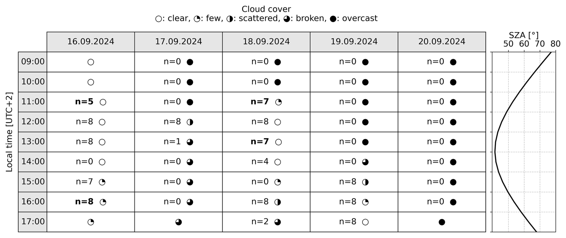
Figure 2 Schedule of the controlled release experiment with the number of overpasses n for each release and a symbol for the average cloud conditions during the release. As the releases started either at '00, '30 or '45, the row label indicates the hour of the release end in local time. If no number of overpasses is given, no release took place during that time window. Bold entries indicate releases observed at all altitude levels; otherwise, observations were limited to 4200 and 3300 ft. The right-hand panel shows the average SZA for each hour.

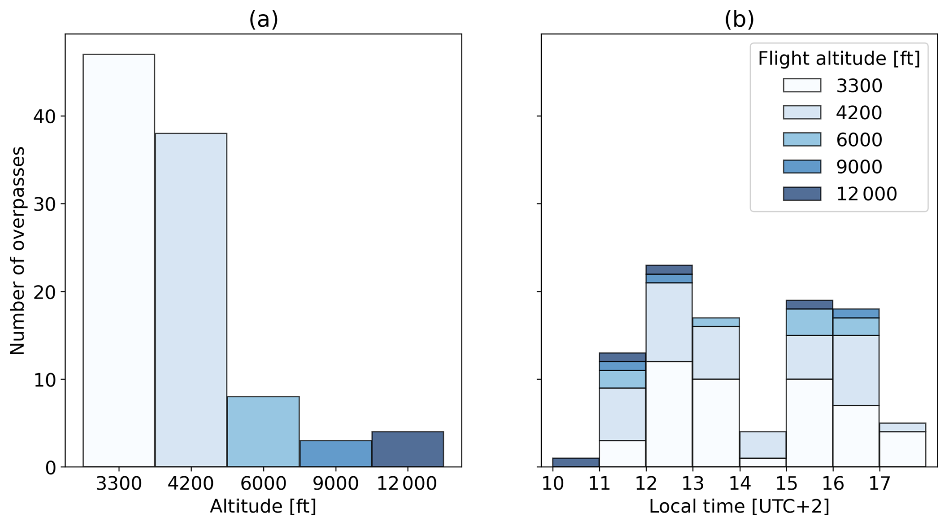
Figure 3 (a) Number of overpasses at five different altitudes above mean sea level. (b) Number of overpasses at different hours of the day.

3.2 Examples of plume images

Figure 4 (upper row) presents three optimal examples of plumes resulting from three different releases. The plumes appear largely linear, with minimal influence from turbulence, which is favourable for emission estimation. For stronger sources, retrieval noise is barely noticeable, but at lower intensities – such as the 26.4 kg CH₄ h⁻¹ release – it can interfere with the plume signal and hinder accurate attribution of enhanced pixels (see Sect. 3.5.5).

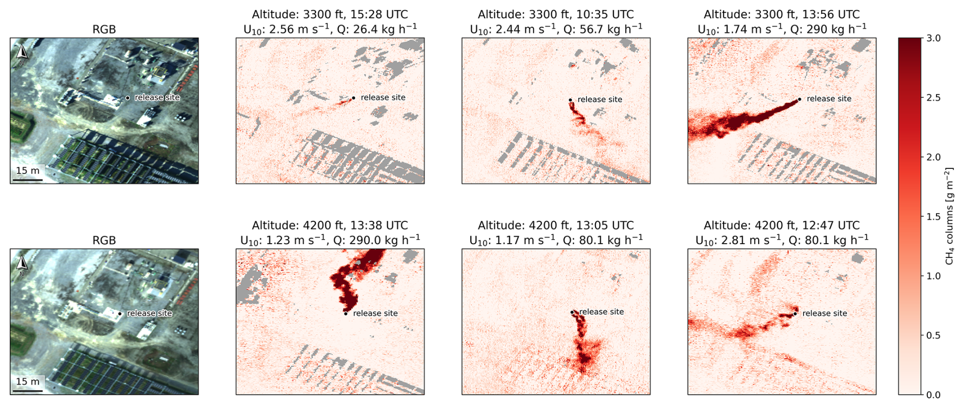
Figure 4 Upper row: Linear CH₄ plumes from release events with 26.4, 56.7 and 290 kg CH₄ h⁻¹, observed at 3300 ft at an average spatial resolution of 0.40 to 0.43 m. Lower row: Turbulent CH₄ plumes from release events with 290 and 80.1 kg CH₄ h⁻¹, observed at 4200 ft at an average spatial resolution of 0.48 m.

The lower row in Fig. 4 shows three turbulent plumes observed during overpasses at 4200 ft, where local enhancements caused by turbulent eddies are clearly visible. In these cases, the CSF method outperforms the IME approach, as the effect of turbulence is reduced through averaging across multiple cross-sections.

In addition to challenging conditions, there was also a case where turbulence impeded emission estimation, shown in Fig. 5. A change in wind direction prior to the overpass appears to have caused a large, dispersed “blob” of CH₄ enhancements. Since these conditions violate the steady-state assumption, this case was excluded from emission estimation.

Figure 5 CH₄ plume from release events with 52.94 kg CH₄ h⁻¹, observed at 3300 ft at a spatial resolution of 0.42 m.

3.3 Detection limit

The median noise level of CH₄ maps was estimated to be around 450 ppm m or 0.3 g CH₄ h⁻¹ for the data of the controlled release experiment. Out of 100 overpasses, plumes were detected on 68 instances (Fig. 6). In the most favourable case, the smallest observed plume corresponded to a 1.45 kg CH₄ h⁻¹ release at U₁₀=0.76 m s⁻¹ and a flight altitude of 4200 ft, representing the best-case detection limit for AVIRIS-4. Under typical conditions, plumes from releases of 5.5 kg CH₄ h⁻¹ and above were consistently detected at altitudes ≤4200 ft, with the exception of two overpasses where shadows from surface infrastructure obscured the signal. At higher flight altitudes (6000–12 000 ft), detection performance was more constrained: for release rates ≤9.23 kg CH4 h⁻¹, only one plume was detected (6000 ft, U₁₀=1.3 m s⁻¹), while the others could not be observed due to the combined effect of higher winds and lower emissions. The original objective of conducting observations at multiple flight altitudes was to determine an altitude-dependent detection limit. However, because the CH₄ release rates were not known in advance, the largest release event captured at all five altitudes was metered at only 9.23 kg CH₄ h⁻¹. This emission rate was below the detection threshold at altitudes above 6000 ft and therefore remained undetectable in those overpasses. For the overpasses below 6000 ft, we computed the probability of detection (PoD) for AVIRIS-4 according to Conrad et al. (2023) as a function of reported emissions Q_rep, U₁₀ and flight altitude $\stackrel{\mathrm{̃}}{h}$ using the flags “detected” and “not detected” by optimising the predictor and inverse link functions. This resulted in the following PoD function which is plotted in Fig. 6.

$$\begin{array}{}\text{(21)}& \mathrm{PoD}=\mathrm{1}-{\left(\mathrm{1}+\left(\mathrm{1.03}\times {\mathrm{10}}^{\mathrm{10}}\right){\displaystyle \frac{\left(\mathrm{5.18}\times {\mathrm{10}}^{\mathrm{8}}\right)Q^{\mathrm{1.93}}}{{\left({\displaystyle \frac{\stackrel{\mathrm{̃}}{h}}{\mathrm{1000}}}\right)}^{\mathrm{3.88}}{\left(U_{\mathrm{10}}+\mathrm{97.0}\right)}^{\mathrm{9.97}}}}\right)}^{-\mathrm{1.84}}\end{array}$$

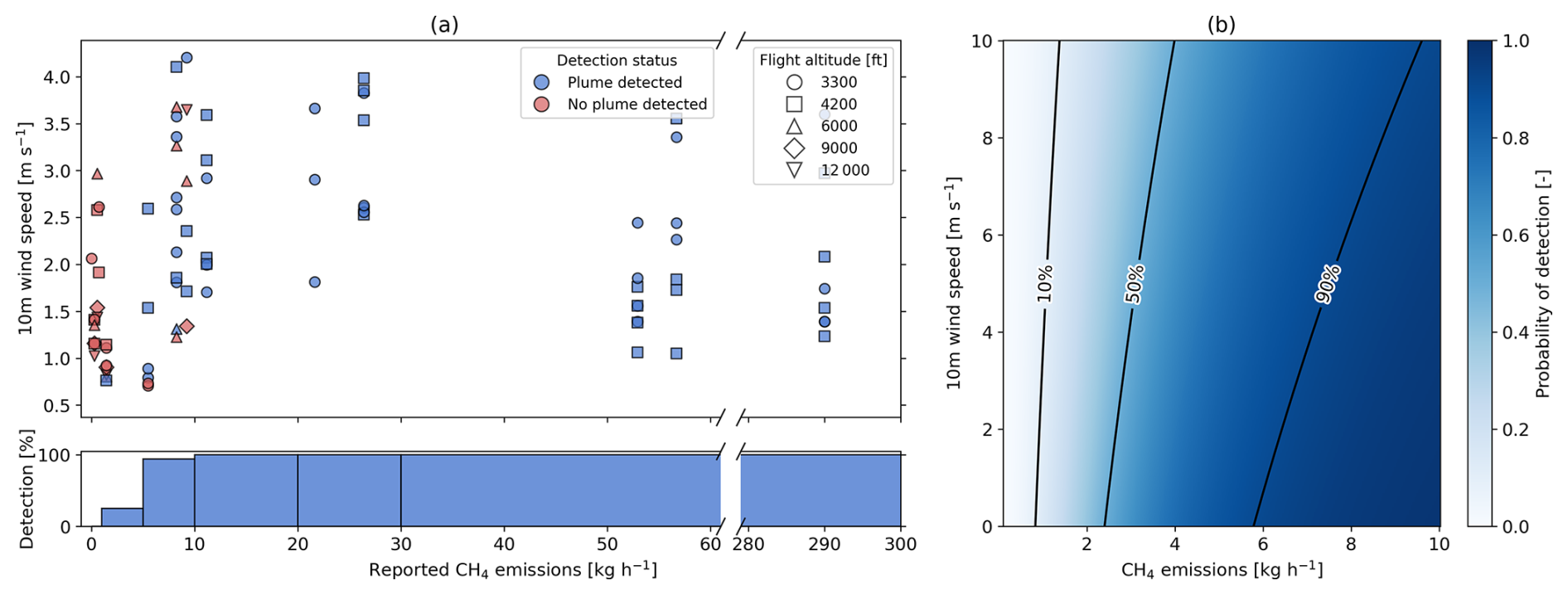
Figure 6 (a) Reported CH₄ emissions vs. on-site lidar wind measurement at 10 m. (b) Probability of detection for a flight altitude of 1000 m. above mean sea level using Eq. (21).

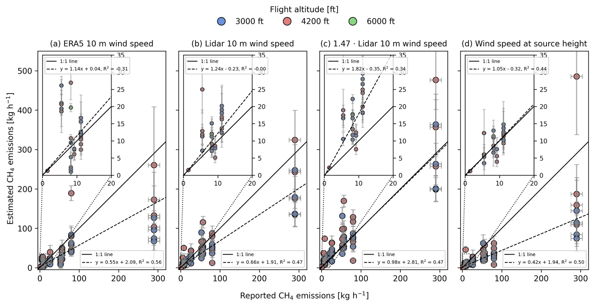
Figure 7 Comparison between reported and estimated CH₄ emissions using (a) ERA5 10 m wind speeds, (b) lidar 10 m wind speeds, (c) effective wind speeds using 1.47×U₁₀ according to Varon et al. (2018) and (d) effective wind speeds at source height as described in Sect. 2.5. Insets enlarge the low-emission range and have an independent fit to the emission estimates. It is important to note that the R² value represents the coefficient of determination of the weighted regression, which can take negative values.

3.4 CH₄ emission estimation

We were able to estimate the emission from 67 of the 68 detected plumes, 54 of which were estimated using the CSF method and 13 using the IME method. Figure 7 shows the reported versus estimated CH₄ emissions using four different wind speed inputs. As outlined in Sect. 2.5, the initial CH₄ emission estimates were calculated using ERA5 U₁₀, shown in subplot (a) of Fig. 7. This approach yields a relatively weak correlation, with a fitted slope of only 0.53 and an R² value of 0.55. Replacing ERA5 data with lidar-measured U₁₀ in subplot (b) of Fig. 7 substantially improves the agreement, increasing the slope to 0.65 and an R² value of 0.73. This highlights the limitations of reanalysis wind data for accurate emission quantification (further shown in Fig. A1). As a result, the use of ERA5 introduces both correlated and uncorrelated uncertainties in emission estimates that are difficult to quantify or correct.

Even when using on-site lidar wind speeds (Fig. 7b), biases remain: emission rates for small release events tend to be overestimated, while large releases (e.g. at 80.1 and 290 kg CH₄ h⁻¹) are significantly underestimated. This behaviour can be explained by plume dynamics: Small release events result in short plumes which remain near the emission height (<10 m for all releases), making the use of U₁₀ prone to overestimation. In contrast, large releases produce longer plumes that undergo greater vertical mixing. The actual effective transport height may thus be above 10 m, resulting in an underestimation of emissions when using U₁₀. Additional influencing factors are specific to the release equipment, such as the outlet ejection velocity and whether the emission was oriented horizontally or vertically.

These limitations highlight the importance of estimating an effective wind speed (U_eff) that accounts for both source height and vertical mixing. Subplots (c) and (d) in Fig. 7 compare two approaches: the method of Varon et al. (2018), which accounts only for vertical mixing, and the method developed in this study, which accounts only for source height. In subplot (c), the overall fitted trend lies close to the 1:1 line, but the estimates for small releases are substantially worse than when using U₁₀. This reflects the fact that Varon et al. (2018) derived the linear relationship between U₁₀ and U_eff for GHGSat, which has a coarser spatial resolution (50 × 50 m). At that scale, plumes have more time to mix vertically and are therefore transported by winds stronger than U₁₀. In contrast, subplot (d) shows a poorer overall trend than (c) due to the strong influence of large release events, but the estimates for small releases improve considerably. This suggests that short plumes are well captured because they remain close to the emission height, whereas vertical mixing is insufficiently accounted for in the case of larger releases.

To further investigate this hypothesis of strong vertical mixing, we incorporated lidar wind speeds at 20 and 38 m and calculated the uncertainty-weighted root mean squared error (RMSE) and relative mean bias error (MBE) between estimated and reported CH₄ emissions, as shown in Fig. 8. The results confirm that using U_src substantially improves emission estimates for low intensity release events. For release events above 30 kg CH₄ h⁻¹, however, using U_src tends to underestimate emissions and performs worse than estimates based on U₁₀, U₂₀ and U₃₈. Although the relative MBE decreases for larger releases, the high relative RMSE indicates substantial variability around the true values. This pattern may reflect the greater influence of turbulence on longer plumes compared to shorter ones.

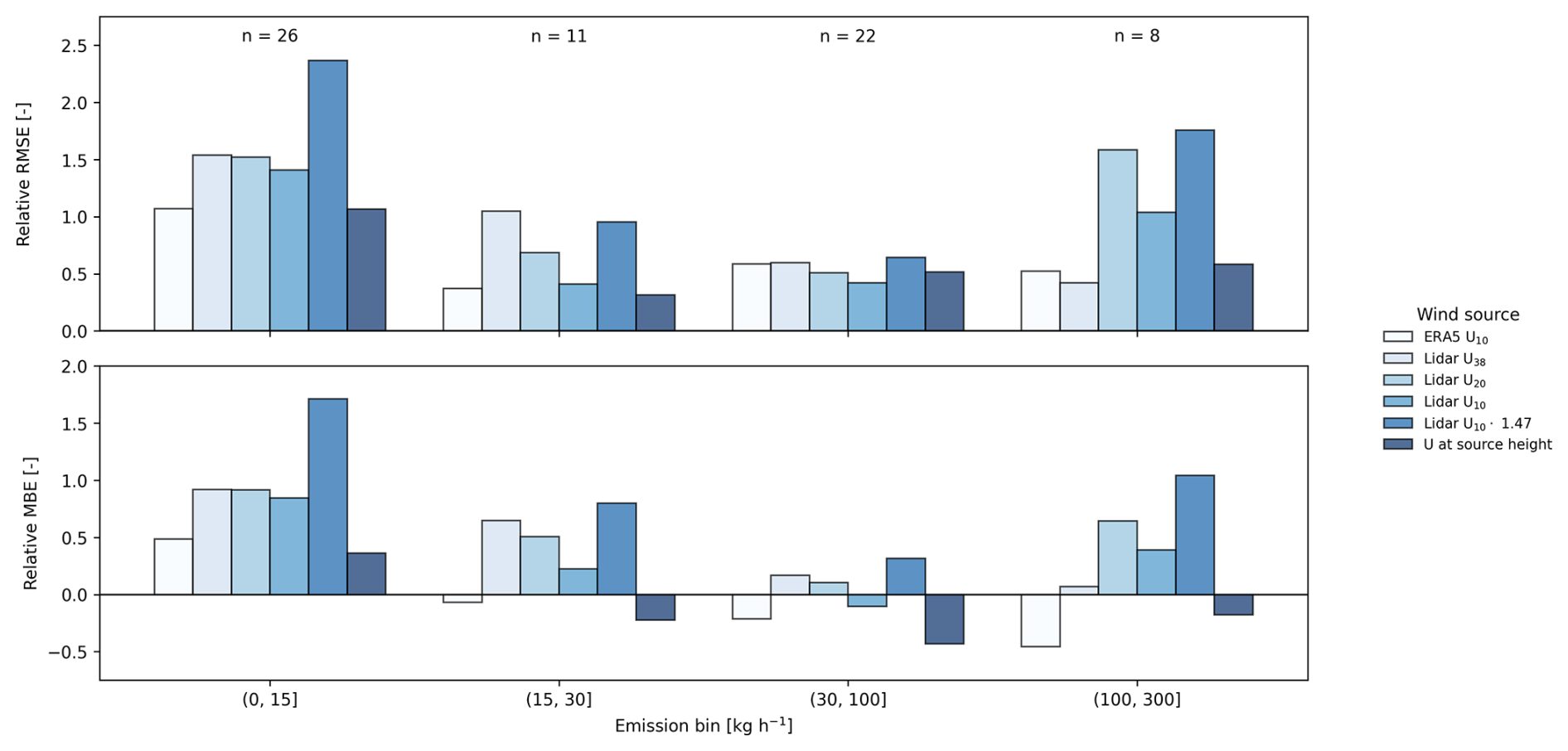
Figure 8 Mean relative root mean squared error (RMSE) and relative mean bias error (MBE) between estimated and reported CH₄ emissions across emission bins.

In addition to source strength and therefore plume length, absolute wind speed appears to significantly influence the accuracy of emission estimates. This is illustrated in Fig. 9, which shows the scaling factor required to align estimated emissions with reported values as a function of (a) plume length and (b) effective wind speed. While subplot (a) of Fig. 9 supports the previously discussed hypothesis regarding plume length, subplot (b) reveals that lower wind speeds are associated with larger and more variable scaling factors. This observation aligns with the findings of Varon et al. (2018); Sánchez-García et al. (2022); McManemin (2025), who reported reduced accuracy in emission estimates across various techniques under low wind speed conditions. This is likely due to the increased variability typically observed at lower wind speeds. In contrast, we did not observe larger scaling factors for larger coefficients of variation (CoV) in wind direction in subplot (c) of Fig. 9 as discussed in McManemin (2025). The reason for this is that our method does not depend on wind direction, as we do a nearly instantaneous measurement. The large spread in angles between the wind direction and the curve fitted to the plume in subplot (d) further highlights the strong influence of wind turbulence on the observed plumes.

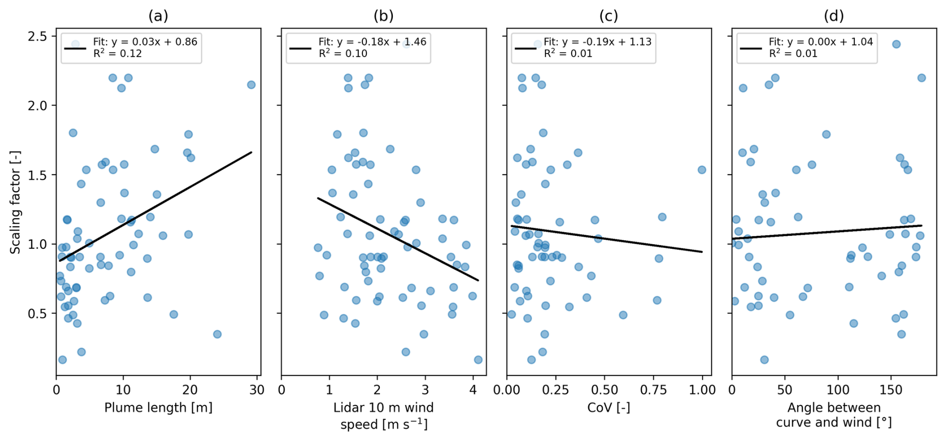
Figure 9 Correlation of (a) plume length, (b) 10 m wind speed, (c) Coefficient of Variation (CoV) and (d) angle between plume curve and wind direction with the scaling factor required to align estimated CH₄ emissions using lidar 10 m wind speeds with reported values.

This hypothesis is further supported by individual cases where estimated emissions diverge from reported values, as illustrated in Fig. 10. Subplot (d) shows that the CH₄ fluxes across different cross-sections fluctuate strongly between 100 and 200 kg CH₄ h⁻¹ due to turbulent wind, likely reflecting both temporal variability in wind speed and changes in plume height that exposed it to different wind regimes. In such cases, one might consider using only CH₄ enhancements close to the source, such as those from the first cross-section, where U_eff is expected to better approximate the wind speed at source height. However, this example shows that even this approach leads to underestimation, indicating that the measured wind speeds do not accurately reflect actual wind conditions. An analysis of the wind speed during the two minutes of the overpass reveals that U₁₀ varies between 1 and 3 m s⁻¹. For comparison, a 20 m plume under a 1 m s⁻¹ wind has a residence time of about 20 s, which matches the sampling interval of the wind lidar. As a result, the wind speed fluctuations visible in the plume cannot be resolved by the lidar, and the underestimation can likely be attributed to larger-than-expected temporal variability that is not captured at the instrument's temporal resolution.

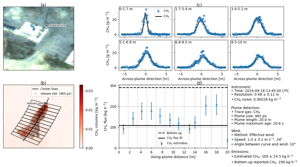
Figure 10 (a) RGB image of the release location, (b) CH₄ map showing the detected plume and 12 cross-sections, (c) Gaussian fits to the CH₄ columns from the first and last three cross-sections, (d) along-plume flux of all cross-sections and retrieval metadata.

The analysis of uncertainty contributions to total emission estimate uncertainty (Fig. A2) indicates that wind speed is the dominant factor for both the CSF and IME methods. Most of this contribution arises from the natural variability of wind speed, with additional influence from uncertainty in the effective wind speed. In comparison, measurement errors in wind speed account for only a minor portion of the overall uncertainty.

Lastly, one source of deviation between estimated and reported CH₄ emissions is the presence of cloud shadows over the release site as shown in Sect. 3.5.3, leading to the strong underestimations of the 80.1 kg CH₄ h⁻¹ release event observed in Fig. 7. Despite this underestimation, the plumes were still reliably detected, indicating that observations under suboptimal cloud conditions can still be valuable e.g. for leak detection.

3.5 Factors affecting the CH₄ retrievals

3.5.1 Spatial resolution

Figure 11 shows examples of AVIRIS-4 RGB images and CH₄ maps of the release site acquired at 12 000, 9000, 6000, 4200, and 3300 ft in the afternoon of the 16 September. The across-track resolutions are 2.0, 1.5, 1.0, 0.7, and 0.5 m, while the along-track resolution is approximately 0.4 m. For the overpasses at 12 000 and 6000 ft, the across-track resolution is represented on the x-axis, whereas for the others it is represented on the y-axis. Black circles indicate an artefact caused by a white object located at the release site. This artefact arises because, first, the reflectance signal appears to correlate with the CH₄ signal, and second, the high albedo of the object leads to increased radiance, which in turn produces an artificially elevated enhancement in the CH₄ maps. At higher altitudes (12 000 and 9000 ft), the spatial resolution is too coarse to clearly distinguish this artefact from a true enhancement. The CH₄ plume from the release event with an emission rate of 9.23 kg CH₄ h⁻¹ is only visible at higher spatial resolutions during overpasses at 3300 and 4200 ft.

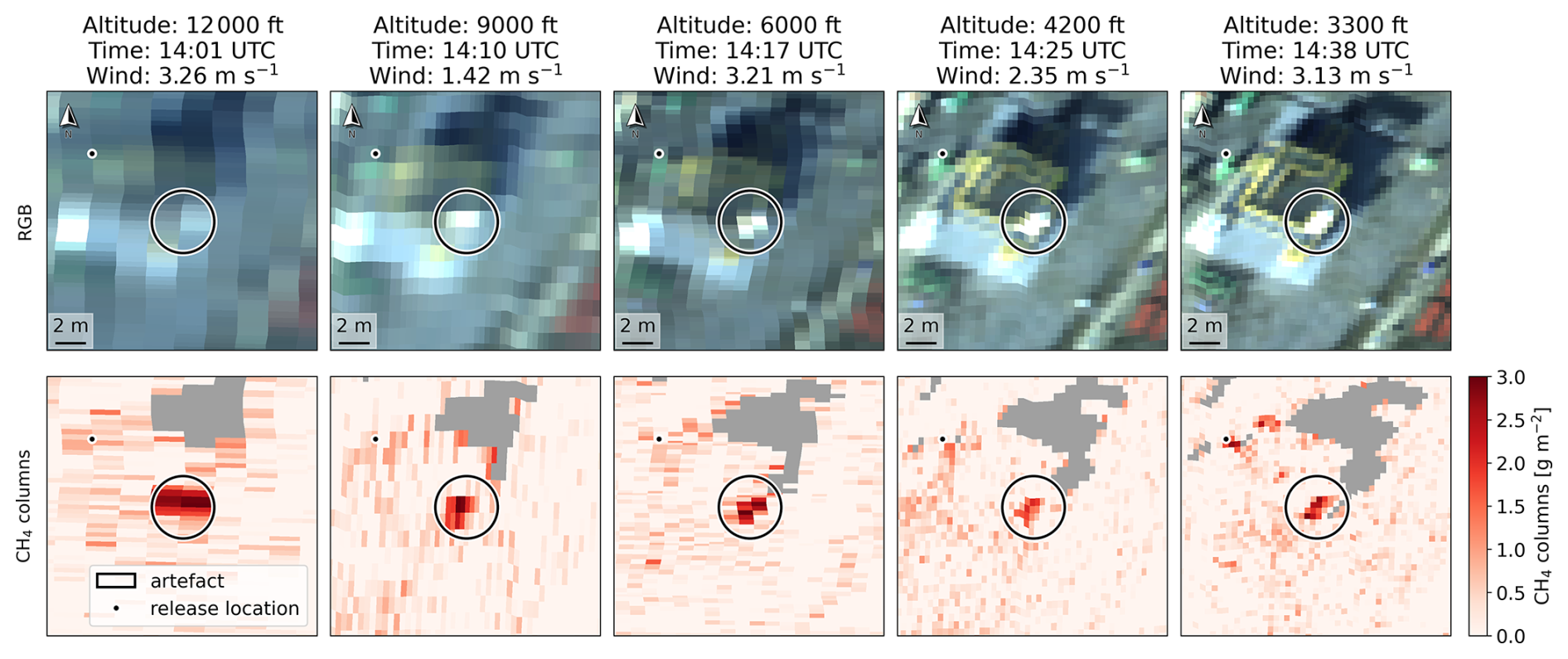
Figure 11 RGB images and CH₄ maps for different flight altitudes with average spatial resolutions of 2.0, 1.5, 1.0, 0.7 and 0.5 m across-track and 0.35 m along-track. All observations are from a release event on the 16 September with reported emissions of 9.23 kg CH₄ h⁻¹.

3.5.2 Cast shadows

The cast shadows of buildings and objects are clearly visible at high spatial resolution. Shadows compromise the CH₄ retrieval, which assumes a non-scattering atmosphere, since light in shadowed areas originates solely from scattering. Therefore, an efficient shadow masking is necessary at these resolutions. Figure 12 shows the effect of the shadow mask for a scene with water bodies and cast shadows and the release site with a nearby photovoltaic plant. It can be seen that the masking of cast shadows and dark surfaces such as solar panels is important to prevent biases in the CH₄ maps which would interfere with plume detection. Furthermore, in instances where the plume coincides with shadowed areas, the artificially elevated enhancements would skew emission estimates. As a result of the shadow mask, CH₄ emissions can also be estimated if the plume is transported over shadowed areas.

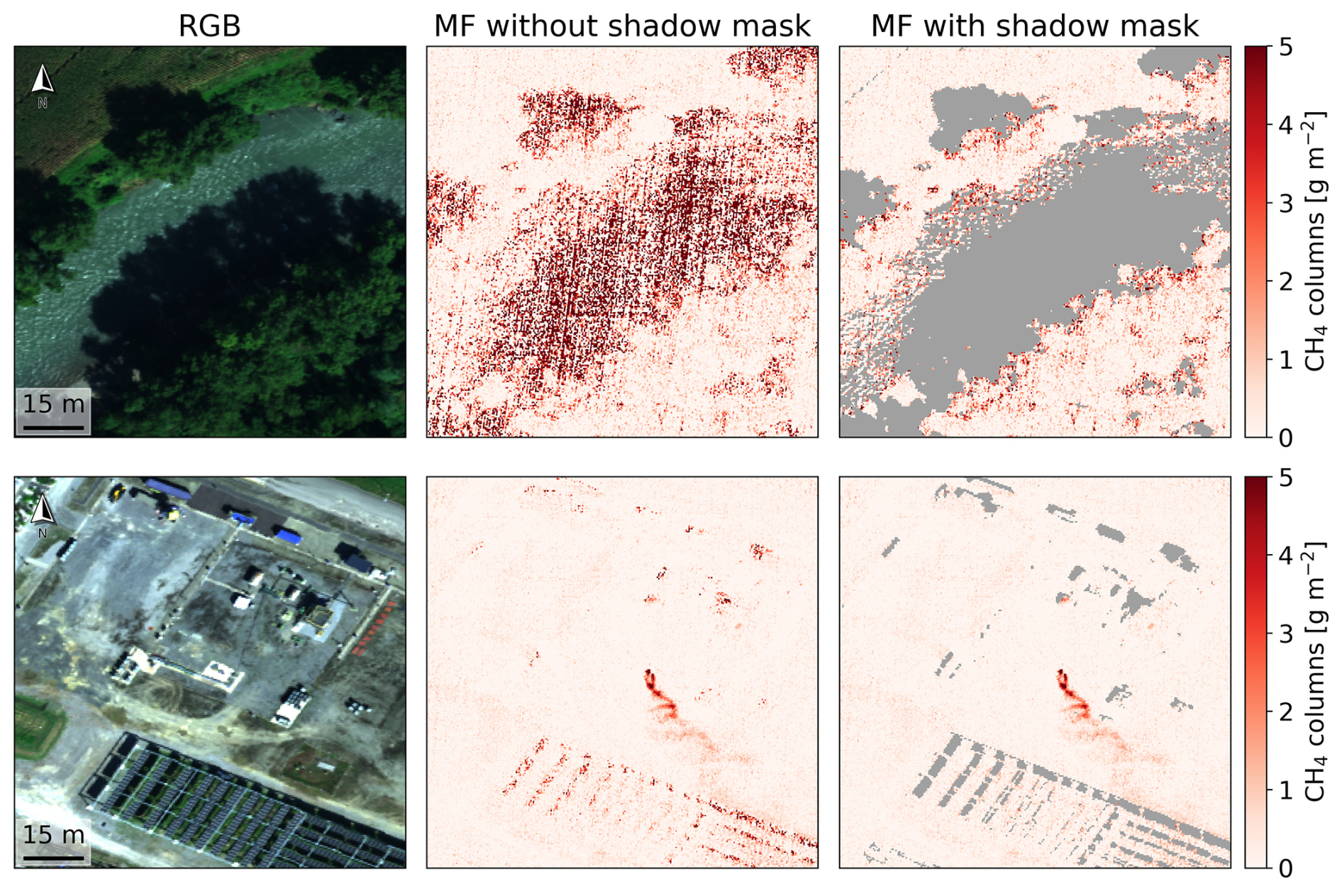
Figure 12 Examples of scenes containing cast shadows and water bodies (upper row) and the release site during a release event with 56.7 kg CH₄ h⁻¹ (lower row), without and with shadow masking.

The downside of shadow masking is that some short plumes of small release events could not be detected because they aligned with shadows. Furthermore, depending on the threshold used for shadow masking, surfaces with low albedos could be masked, preventing the detection of CH₄ emissions.

3.5.3 Cloud shadows

During all eight overpasses of the 80.1 kg CH₄ h⁻¹ release on the 19 September, cloud shadows intersected the flight line while on five out of eight overpasses, cumulus clouds obscured the sun over the release site. Under such conditions, the measured radiance is dominated by scattered light, violating the assumptions used in calculating the target spectrum. Moreover, cloud shadows on the flight line render the mean spectrum $\widehat{\mathit{\mu }}$ unrepresentative of the observed radiance L_obs over the release site. Consequently, subtracting $\widehat{\mathit{\mu }}$ from L_obs in Eq. (2) partially removes the CH₄ signal. This effect is evident in Fig. 13, which contrasts an overpass with obscured sun at 13:00 UTC with a clear-sun overpass at 12:5 UTC. The lower row shows $L_{\mathrm{obs}}-\widehat{\mathit{\mu }}$ over the same plume-free area in both cases. As can be seen, the cloud shadow strongly reduces the signal. As a result, emission estimates for shadowed cases, or for scenes with a substantial fraction of cloud shadows along the flight line, tend to be underestimated. Consequently, a refined retrieval algorithm would be necessary to provide unbiased CH₄ maps and emission estimates.

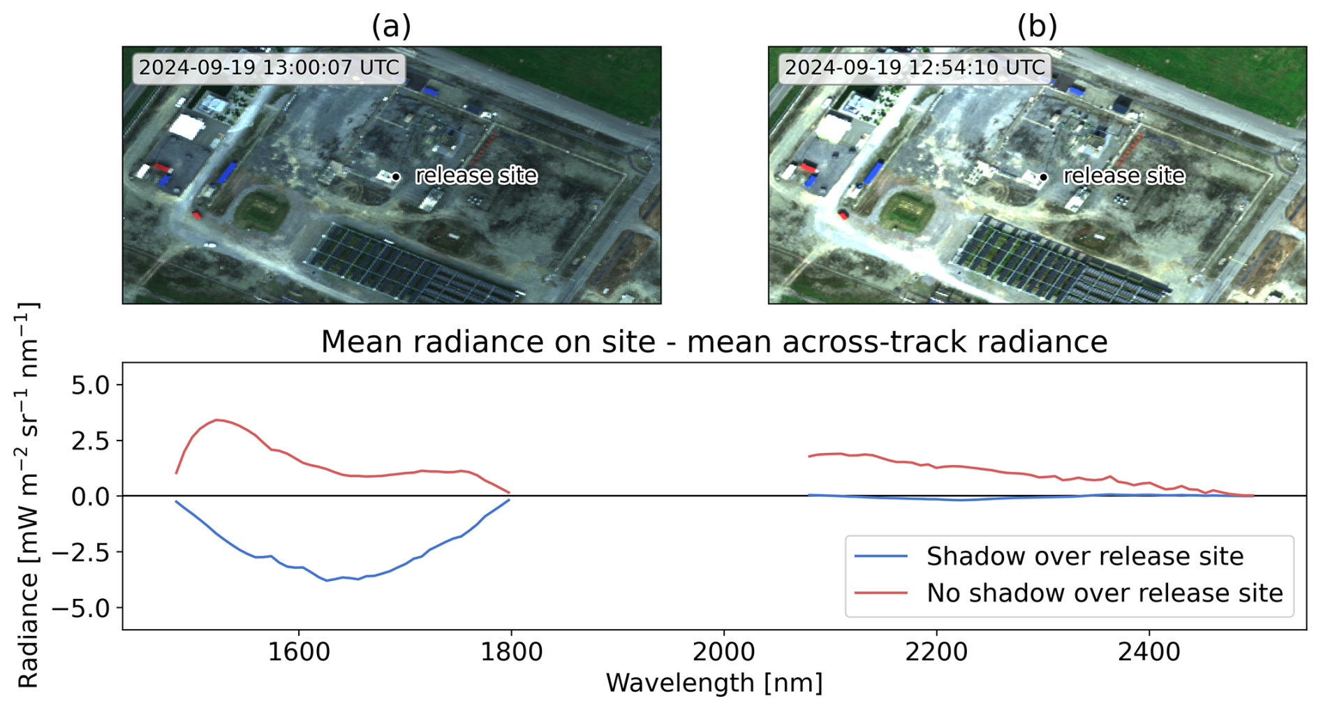
Figure 13 RGB image of 80.1 kg CH₄ h⁻¹ release on the 19 September (a) with and (b) without cloud shadow. The lower row shows the mean $L_{\mathrm{obs}}-\widehat{\mathit{\mu }}$ over the same plume-free area within the wavelength window used for CH₄ retrieval for both cases.

3.5.4 Plume shadows

As a consequence of the unprecedentedly high spatial resolution of AVIRIS-4 and the high SZA for some of the overpasses (see Fig. 2), we discovered that, out of 68 detected plumes, 13 were found to contain two plumes that were occasionally overlapping and occasionally distinct, as illustrated in Fig. 14.

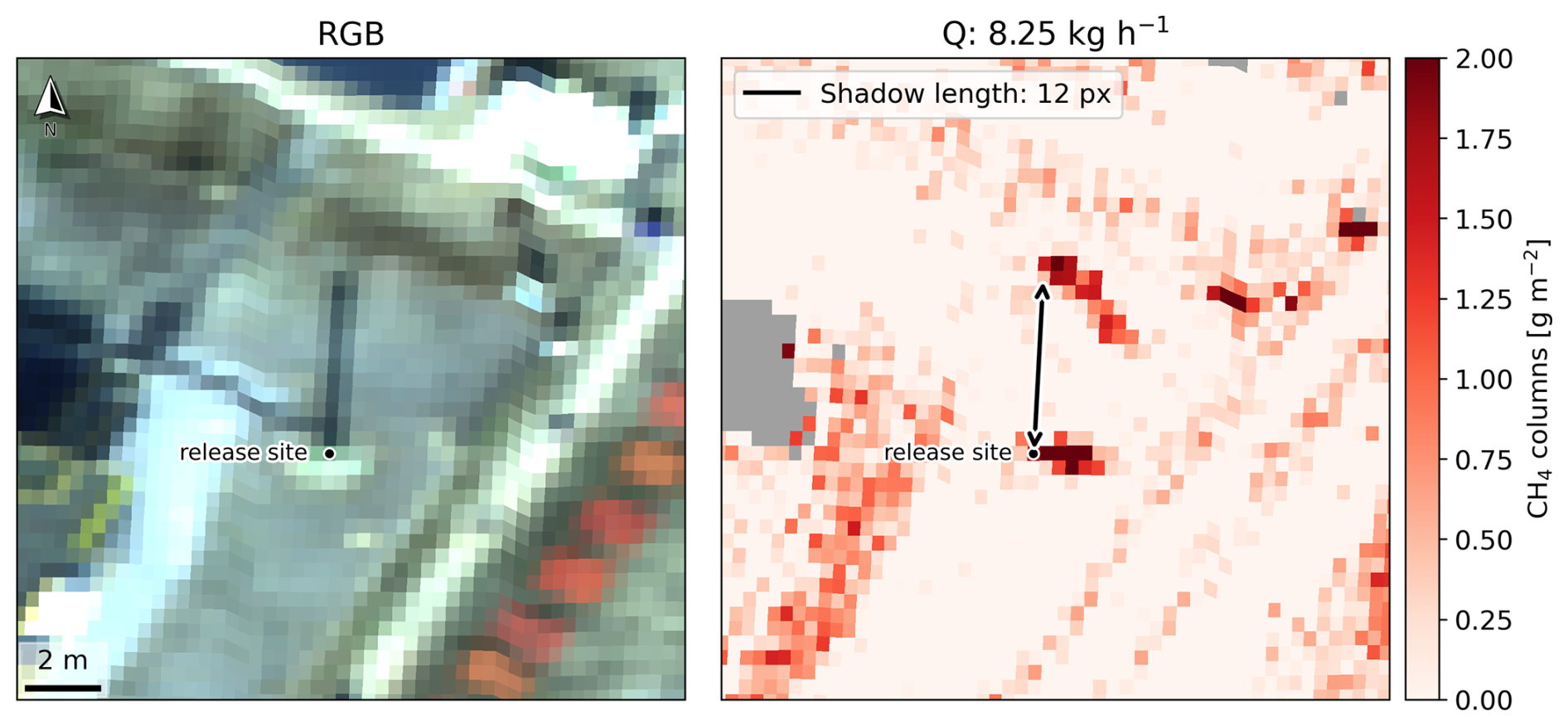
Figure 14 Left: RGB image of the study site with a marker on the release location at 6.5 m above ground. Right: CH₄ map of the study site with two plumes visible.

This phenomenon can be explained as plume shadows: One plume appears at the actual release location and corresponds to the CH₄ absorption signal of the light path that first travels from the sun to the ground and, after being reflected, passes through the plume. The second plume is observable at the upper end of the shadow cast by the pole of the source. This plume corresponds to the absorption signal of the light that first passes through the plume, is then reflected from the ground and reaches the sensor without passing through the plume a second time. This phenomenon has been shown in simulations by Schwaerzel et al. (2020) and first observed by Sánchez-García et al. (2022). It is important to note that the effect of light passing through the plume only once instead of twice occurs under all conditions with sufficiently high SZA. For sensors with coarse spatial resolution, however, the plume and its shadow cannot be resolved separately and have therefore never been explicitly considered in CH₄ retrieval or emission estimation prior to this study. To correct for plume shadows, we applied the method outlined in Sect. 2.4.4 to the four observed plumes that were clearly separated. This resulted in a mean correction factor of 2.6.

3.5.5 MF vs. LMF

For the analysis of this study we also tested the LMF which was developed by Schaum (2021) and tested in Pei et al. (2023). The plume images using the MF and LMF in Fig. 15 show that smaller enhancements (upper row) can be detected more reliably and accurately using the LMF as worked out in Schaum (2021). In our case, the LMF enabled the detection of a release as small as 1.45 kg CH₄ h⁻¹ at a flight altitude of 4200 ft. This improved detectability can be attributed, in part, to reduced random background variability in the retrieved CH₄ maps, which facilitated more confident identification of the plume signal. However, the LMF also introduces larger systematic biases in background CH₄ values compared to the MF, as evident in both the upper and lower rows of Fig. 15. An analysis of the eigenvalues of the covariance matrices for different surface albedos suggests that these biases are associated with increased sensitivity of the log-transformed radiances to pixels with low SNR, which is the case for albedo surfaces with low albedo. Additionally, we observed that the LMF had little to no effect on CH₄ enhancements for the largest release events in the campaign, such as the 290 kg CH₄ h⁻¹ release. This is likely because our iterative MF already compensates for most of the non-linear absorption associated with high optical depths.

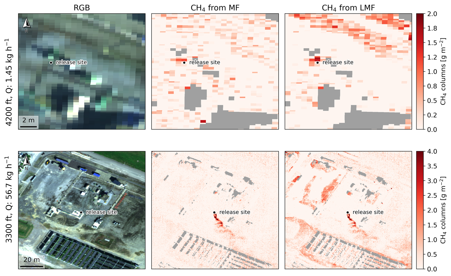
Figure 15 RGB images and CH₄ maps obtained from MF and LMF for release events with 1.45 and 56.7 kg CH₄ h⁻¹, observed at 4200 and 3300 ft. Note that the upper row shows a zoomed-in subsection of the scene to be able to see the short plume.

3.6 Estimating the source height from (plume) shadows

The high spatial resolution of AVIRIS-4 offers the unique opportunity to estimate the height h of an emission source based on the length of the shadow l_s in the RGB image (Fig. 14a) cast by the emission source using trigonometry:

$$\begin{array}{}\text{(22)}& h={\displaystyle \frac{l_{\mathrm{s}}}{\tan \left(\mathrm{SZA}\right)}}\end{array}$$

Alternatively, the height can be estimated in the same way from the horizontal separation of the starting points of the two plumes (Fig. 14b). With increasing distance, the two plumes move together more closely, suggesting that the plume is pushed towards the surface directly after the release. Knowledge of the emission height is an important parameter for emission estimation, as it can be used to determine the effective wind speed, which is a critical input for estimation estimation. In the example shown in Fig. 14 with an SZA of 50° and a spatial resolution of 0.53 m, the emission plume at the stack must be 6.4,± 1.1 m above ground which is in agreement with the true emission height of 6.5 m.

We assume that this technique can be reliably applied only if the measured shadow length exceeds its measurement uncertainty by a sufficient margin. The uncertainty in the shadow length is dominated by pixel discretization at the shadow boundaries, where at most one mixed pixel can occur at both the upper and lower edge of the shadow. Requiring the shadow length to be at least twice this uncertainty ensures that the shadow is sufficiently resolved. Under this criterion, the minimum emission height that can be resolved is given by

$$\begin{array}{}\text{(23)}& h>{\displaystyle \frac{\mathrm{2}\cdot l_p}{\tan \left(\mathrm{SZA}\right)}}\end{array}$$

For the campaign discussed in this study, this minimum height is shown in Fig. 16.

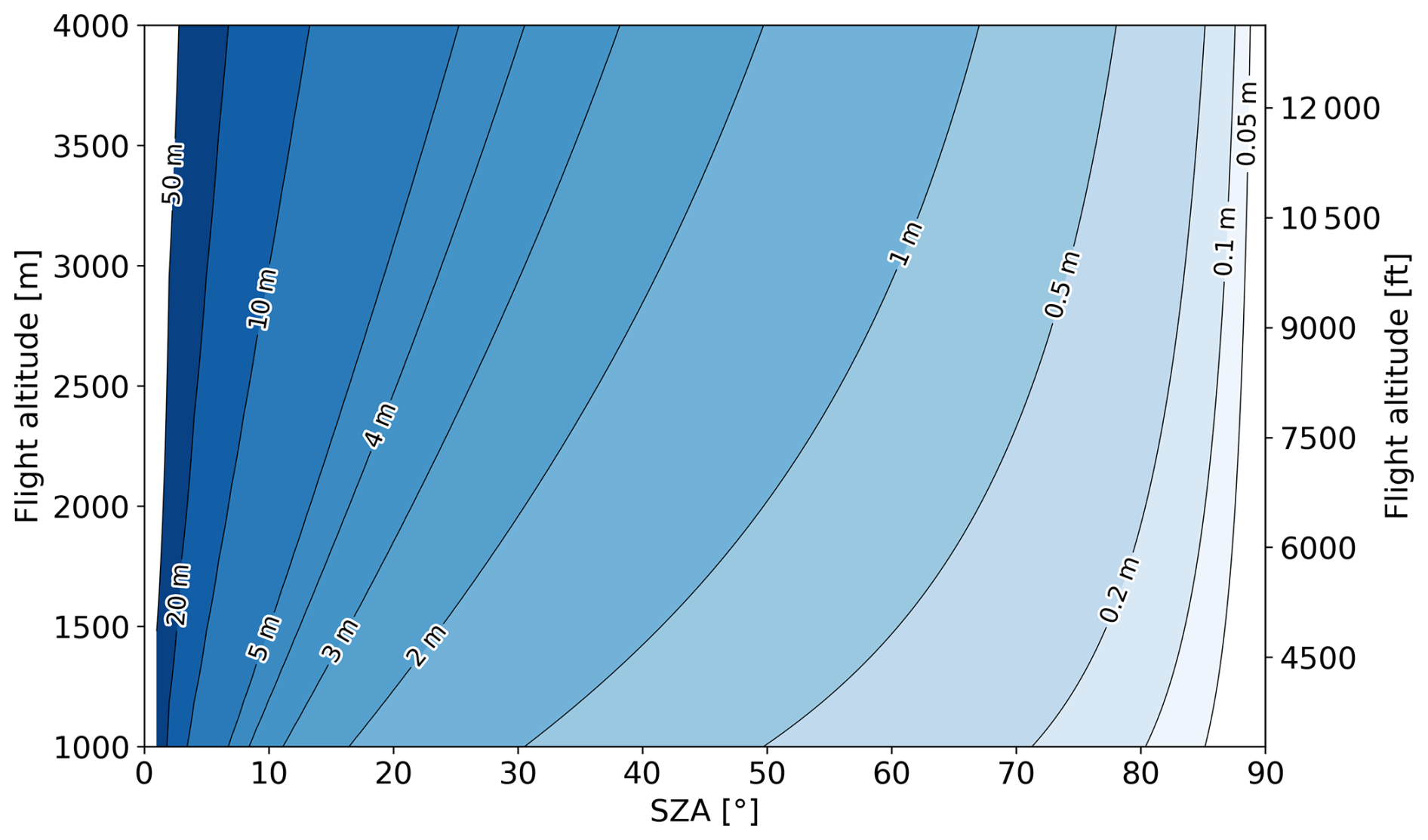
Figure 16 Minimum source height in metres above ground at which shadows of emission sources extend over more than one pixel, shown as a function of SZA and flight altitude above mean sea level.

4 Discussion

4.1 Capabilities and limitations of AVIRIS-4

Following the success of the AVIRIS Classic and AVIRIS-NG sensors in detecting and quantifying CH₄ emissions as demonstrated in numerous previous studies, this study explores the potential of their successor, AVIRIS-4. Although AVIRIS-4 was primarily developed for surface and vegetation studies, our results show that CH₄ columns can be determined with an unprecedentedly high spatial resolution, enabling the detection of short plumes from low intensity sources. In combination with the enhanced SNR, the detection limit is reduced to 5.5 kg CH₄ h⁻¹ under good weather conditions and down to below 1.5 kg CH₄ h⁻¹ under ideal conditions. Because the campaign took place in mid-September, we expect the detection limit could be further reduced under more favourable illumination conditions. As discussed in Sect. 3.3, we were not able to determine an altitude-dependent detection limit for AVIRIS-4, which complicates direct comparisons with other airborne sensors. For instance, studies with AVIRIS-NG operated at altitudes between 3000 and 6000 m report detection limits of 10–16 kg CH₄ h⁻¹ under favourable wind conditions (e.g. Ayasse et al., 2023; Conrad et al., 2023). In our case, the lowest release of 9.23 kg CH₄ h⁻¹ could not be detected at a comparable altitude of 2740 m, likely due to higher wind speeds. This makes it difficult to assess whether and by how much the detection limit has improved. In Thorpe et al. (2016), the lowest detected release was 2.3 kg CH₄ h⁻¹, but at a much lower flight altitude of 430 m and under higher wind speeds of 3–5 m s⁻¹. Kuhlmann et al. (2025) report a detection limit of 15 kg CH₄ h⁻¹ at a flight altitude of 6000 m with wind speeds of 0.5 m s⁻¹. Overall, comparing detection limits across studies is challenging, as they depend strongly on flight altitude, wind speed, and spectral albedo (Conrad et al., 2023).

Decreasing the detection limit is pivotal because low intensity CH₄ sources are more numerous than high-emitting ones (e.g., Williams et al., 2025; Kuhlmann et al., 2025). Consequently, accurate estimates of total CH₄ emissions depend on detecting smaller sources. For instance, based on the best detection limit of AVIRIS-NG of 15 kg CH₄ h⁻¹ reported in Kuhlmann et al. (2025) and the distribution of oil production sites in Romania across the outlined scenarios, AVIRIS-NG was able to detect between 45 % and 62 % of total emissions. In contrast, assuming a detection limit of 5.5 kg CH₄ h⁻¹, AVIRIS-4 would increase this detection coverage to approximately 67 %–81 %. Moreover, the detection limit of 5.5 kg CH₄ h⁻¹ achieved by AVIRIS-4 effectively enables the identification of all point sources listed in the E-PRTR registry, which mandates reporting for emissions exceeding 100 000 kg CH₄ yr⁻¹ (equivalent to 11.4 kg CH₄ h⁻¹) (European Parliament and the Council of the European Union, 2006).

This study, along with comparisons to other airborne imaging spectrometers with higher spectral but lower spatial resolution such as MAMAP2DL (e.g. Krautwurst et al., 2025), demonstrates that the trade-off of higher spatial and slightly lower spectral resolution is beneficial for detecting small-scale CH₄ enhancements from low intensity sources, whose plumes typically extend only a few decimetres to a few metres.

The noise level of the CH₄ maps was estimated as the standard deviation of the retrieved columns over the brightest 50 % of pixels. This resulted in a noise level of AVIRIS-4 of 450 ppm m at an average resolution of 0.5 m which is comparable to reported values of AVIRIS-NG at 5 m resolution for suboptimal illumination conditions (e.g. Borchardt et al., 2021). Such noise levels are expected, given that the campaign was conducted in mid-September under low solar zenith angles (SZAs). In addition, negative values were not masked during the CH₄ retrieval, which increases the apparent noise.

The current study also shows that owing to the higher SNR and higher spatial resolution, emissions can also be detected and estimated with less illumination and under suboptimal surface and atmospheric conditions, which are characterised by inhomogeneous albedo, strong turbulence, cast shadows and cloud shadows (see Sect. 3.1), compared to previous controlled release experiments with AVIRIS-NG (e.g. Thorpe et al., 2016; Duren et al., 2019). For example, the higher spatial resolution allows for a more accurate filtering for shadow pixels and albedo artefacts which, if undetected, could lead to biases in emission estimates, as outlined in Sect. 3.5.2. This capability allows AVIRIS-4 to be effectively applied to built-up sites with heterogeneous surface albedo and cast shadows, conditions commonly encountered around CH₄ sources in the oil, gas, and coal mining sectors.

However, the higher spatial resolution also results in new challenges. One of them is the occurrence of double plumes originating from plume shadows illustrated in Fig. 14. We corrected for this artefact when the true plume and its shadow were clearly separated, but its impact on retrieved CH₄ enhancements requires further analysis. In this context, a recent study by Gorroño et al. (2025) systematically investigated the effect of different observation and illumination geometries on the retrieved CH₄ maps (i.e. parallax effect) and the resulting emission estimates. They showed that large VZAs and SZAs can lead to artificial elongation or compression of plumes along the plume direction. This bias in apparent plume length L directly propagates into emission estimates and likely also occurred in the observations analysed in this study. However, their influence is probably masked by the comparatively large variability in wind speed. Furthermore, Gorroño et al. (2025) found that the parallax effect substantially reduces the PoD due to lower apparent CH₄ enhancements. In their simulations, the PoD varied between approximately 0.5 and 0.8 depending on the angular configuration. For the present study, the influence of parallax effects is likely minor, as the detection outcomes shown in Fig. 6 are primarily controlled by wind speed and flight altitude. The few non-detected plumes with emission rates exceeding 5 kg CH₄ h⁻¹ at low wind speeds are instead attributable to overlaps with retrieval artefacts. Gorroño et al. (2025) also demonstrated that when the effective wind speed U_eff is calibrated against the 10 m wind speed U₁₀ using L, biases in L translate into systematic errors in the calibration itself. As a consequence, emission estimates exhibit errors below 10 % for mid-latitude summer conditions, but can reach up to 30 % for wintertime observations. In the context of this study, the parallax-induced bias in U_eff is only relevant for emission estimates derived using the U_eff parametrisation of Varon et al. (2018) and does not affect estimates based on wind speeds at the source height. To mitigate the effect of viewing geometry, Gorroño et al. (2025) recommended to explicitly account for observation and illumination geometry in the planning of flight paths for airborne sensors and to calibrate U_eff using plume simulations that match the angular configuration (“train as you measure”). Overall, additional work is needed to correct for the parallax effect, especially as this phenomenon also affects instruments with coarser spatial resolution even if they do not spatially resolve the plume shadow (Schwaerzel et al., 2020).

A second challenge that arises with higher spatial resolution are the higher per-pixel enhancements for larger sources. As a result, the linearisation of the unit absorption spectrum around α=0 no longer holds and assumed enhancements for the calculation of the absorption spectrum have greater influences on the retrieved enhancements. Therefore, careful selection of the assumed enhancements, e.g. with the iterative approach used in this study, is essential.

Lastly, the current study shows mixed results when using the LMF introduced by Schaum (2021). On the one hand, the proposed improvement for the detection of weak plumes was also observed in this study and lowered the detection limit even under challenging conditions. On the other hand, the LMF increased local biases in the retrieved CH₄ maps which we attribute to the amplification of noise by the log-transform in pixels with low SNR, caused by low albedo. This spatially more heterogeneous background can obscure small enhancements or produce false detections. In contrast to Schaum (2021), we did not observe an improved performance of the LMF for large release events. The iterative MF applied in our study seems to successfully account for most non-linear absorption in pixels with large CH₄ enhancement. Therefore, further systematic analyses will be required to develop approaches that reduce or correct for this noise amplification in the LMF. Other approaches, such as WFM‑DOAS (e.g. Borchardt et al., 2021), may also help better account for non‑linear effects arising from strong emission sources. However, they are computationally more expensive than the MF and tend to work better for sensors with higher spectral resolution.

4.2 Wind speed estimation

As seen in Sect. 3.4, estimated emissions linearly depend on the wind speeds used. Therefore, accurate estimates of wind speeds are crucial for accurate emission estimates. Additionally, our analysis demonstrated that uncertainties in wind speeds contributed disproportionately to the uncertainty of the estimated emissions. Based on the analysis of this study, the wind speed representation error (σ_repr), uncertainties in effective wind speed (σ_eff) and instrument precision (σ_inst) likely need to be revised upward. Consequently, building on the understanding of wind speed inputs (see Sect. 4.2.1), future research on emission estimation from remote sensing data should prioritise methods for deriving the effective wind speed that governs plume transport (see Sect. 4.2.2).

4.2.1 Source of wind speed estimates

As clearly illustrated in Fig. A1, near-surface winds can be be highly variable and gusty. We frequently found that U₁₀ measured by the lidar varied between 1.0 and 3.0 m s⁻¹ within one minute. These rapid fluctuations highlight that reanalysis wind fields are insufficient for high-resolution emission estimates with new-generation sensors, as they can introduce substantial biases. A high-resolution model may be able to represent this gustiness more realistically in a statistical sense, but capturing the actual wind conditions at the moment of the overpass remains practically impossible. Alternatively, wind speed data from existing measurement networks could be used for emission estimation. However, these networks have varying data quality and might not be available in the vicinity of a CH₄ source. Therefore, one could employ mobile instruments as it was used for the controlled release experiment in the current study. Even if this would provide the most accurate estimate of the wind speed, setting up wind speed instrument would negate the advantage of remote sensing instruments which is to image extensive areas and estimate the emissions of a large number of sources. Additionally, the current analysis has shown that under turbulent conditions, wind speed representation errors can be substantial, even when wind measurements are taken just 100 m from the source. Therefore, the best approach would be to measure wind speed profiles in tandem with imaging spectrometry, e.g. by using an airborne wind lidar as investigated in Thorpe et al. (2021).

4.2.2 Effective wind speeds

In addition to determining the small-scale and short-term wind speeds, a further challenge is to determine the effective wind speed at which the plume was transported. Although an increasing number of studies attempt to derive U_eff from model simulations (e.g. Varon et al., 2018; Guanter et al., 2021; Sánchez-García et al., 2022; Ayasse et al., 2023; Guanter et al., 2025), none has systematically investigated the effect of emission height, atmospheric stability or surface roughness on U_eff. Moreover, existing simulations lack the spatial and temporal resolution required for AVIRIS-4 applications. To advance our understanding of the effective wind speed, high-resolution model studies are needed to analyse the impact of the aforementioned factors. Ideally, these results could be parametrised to estimate the effective wind speed based on known driving factors. While estimates for the 3D wind field, surface roughness and heat fluxes could be obtained from regional weather prediction models, information about the emission height could be obtained directly from AVIRIS-4 imagery as outlined in Sect. 3.6. Another innovative approach has recently been demonstrated in Eastwood et al. (2025) with AVIRIS-3 where a single plume was observed multiple times during one overpass by adjusting the flight path of the aircraft. Specifically, the aircraft ascended while approaching the plume, maintained a level trajectory while flying directly over it, and then descended after passing it. From the resulting three images, the plume velocity was estimated by calculating optical flow vectors for consecutive CH₄ images. While this method proved to significantly improve the estimates of the effective wind speed compared to reanalysis data and on-site wind lidar data, it requires a-priori knowledge of the source location to plan the required flight manoeuvres. One workaround would be to use real-time in-flight retrieval of CH₄ (e.g. Thompson et al., 2015) in combination with pitching AVIRIS-4 using the already installed stabilisation platform. Alternatively, machine learning based models could be used to estimate trace gas emissions either directly from radiance data (e.g. Joyce et al., 2023; Rouet-Leduc and Hulbert, 2024) or from plume images (e.g. Jongaramrungruang et al., 2022; Bruno et al., 2024; Ouerghi et al., 2025; Plewa et al., 2025). These approaches have recently shown that it is possible to infer emission rates without explicitly relying on external wind data. Their main advantages are that they can, just as the other approach outlined above, bypass wind speed uncertainties and additionally, provide rapid and automated emission estimates at large scales. While these models are very promising, they are still limited in their representativeness due to a lack of wind speed information within a single image. Furthermore, they provide limited interpretability and their uncertainty quantification is still less mature than for the traditional approaches based on the mass balance.

5 Conclusions

Detecting and quantifying the emissions from a large number of sources is essential for obtaining accurate inventories of CH₄ emissions. The current study shows that AVIRIS-4 can be used for the improved detection of CH₄ emissions and subsequent quantification. The combination of high spatial resolution with the unprecedentedly high SNR of AVIRIS-4 decreases the detection limit of AVIRIS-4 to below 5.5 kg CH₄ h⁻¹ under good weather conditions and down to 1.5 kg CH₄ h⁻¹ under ideal conditions. This is below the 10–16 kg CH₄ h⁻¹ detection limits reported for its predecessor AVIRIS-NG in previous studies. In practice, AVIRIS-4 therefore extends the range of reliably detectable point sources by approximately a factor of two to three relative to AVIRIS-NG when flown at low altitudes, which effectively enables the identification of all point sources listed in the E-PRTR registry. As a result, previously undetected low intensity and dispersed sources can be identified and accounted for in emission budgets. We demonstrate that the high spatial resolution of AVIRIS-4 enables its effective use under challenging conditions and in heterogeneous environments, which are frequently encountered in real-world applications. Furthermore, we show how high-resolution AVIRIS-4 data can be used for the estimation of the source height which is critical information when estimating the effective wind speed. As with earlier sensors and algorithms, emission estimation with AVIRIS-4 is affected by uncertainties in the estimation of the effective wind speed, especially at the short length and timescales presented in this study. Overall, this study highlights that AVIRIS-4 represents a significant step forward in airborne methane remote sensing, offering unprecedented sensitivity to low-intensity sources under challenging conditions. At the same time, it underscores the importance of advancing wind speed estimation techniques and improving retrieval strategies to fully exploit the sensor’s capabilities. Future work should therefore focus on integrating AVIRIS-4 observations with dedicated wind measurements and adapting the CH₄ retrieval algorithm to the unprecedentedly high spatial resolution.

Appendix A: Additional figures and tables

Figure A1 reveals substantial systematic deviations, particularly during daytime, likely caused by small- to mesoscale atmospheric circulations influenced by local terrain. Such features are not captured by the relatively coarse spatial (0.25°×0.25°) and temporal resolution of ERA5. Furthermore, ERA5 fails to resolve turbulent fluctuations in near-surface winds that are evident in lidar observations.

Figure A2 shows that the uncertainty in the wind speed σ_U contributes 99.4 % to the total uncertainty of the estimated emissions σ_q for the CSF and 91.3 % for the IME. σ_U in turn consists 90.4 % of natural wind speed variability σ_var.

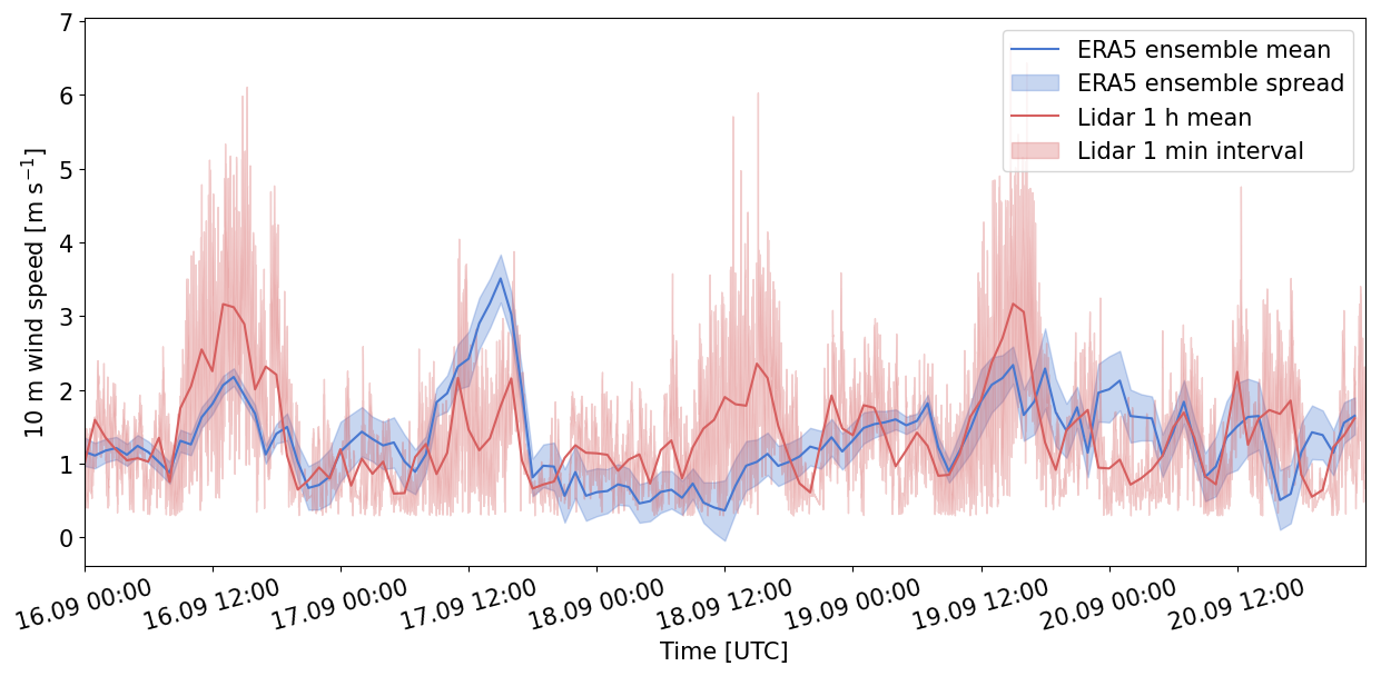
Figure A1 ERA5 U₁₀ vs. on-site lidar U₁₀. The blue shaded area represents the ERA5 ensemble spread while the red shaded area depicts the min and max wind speed for 1 min intervals.

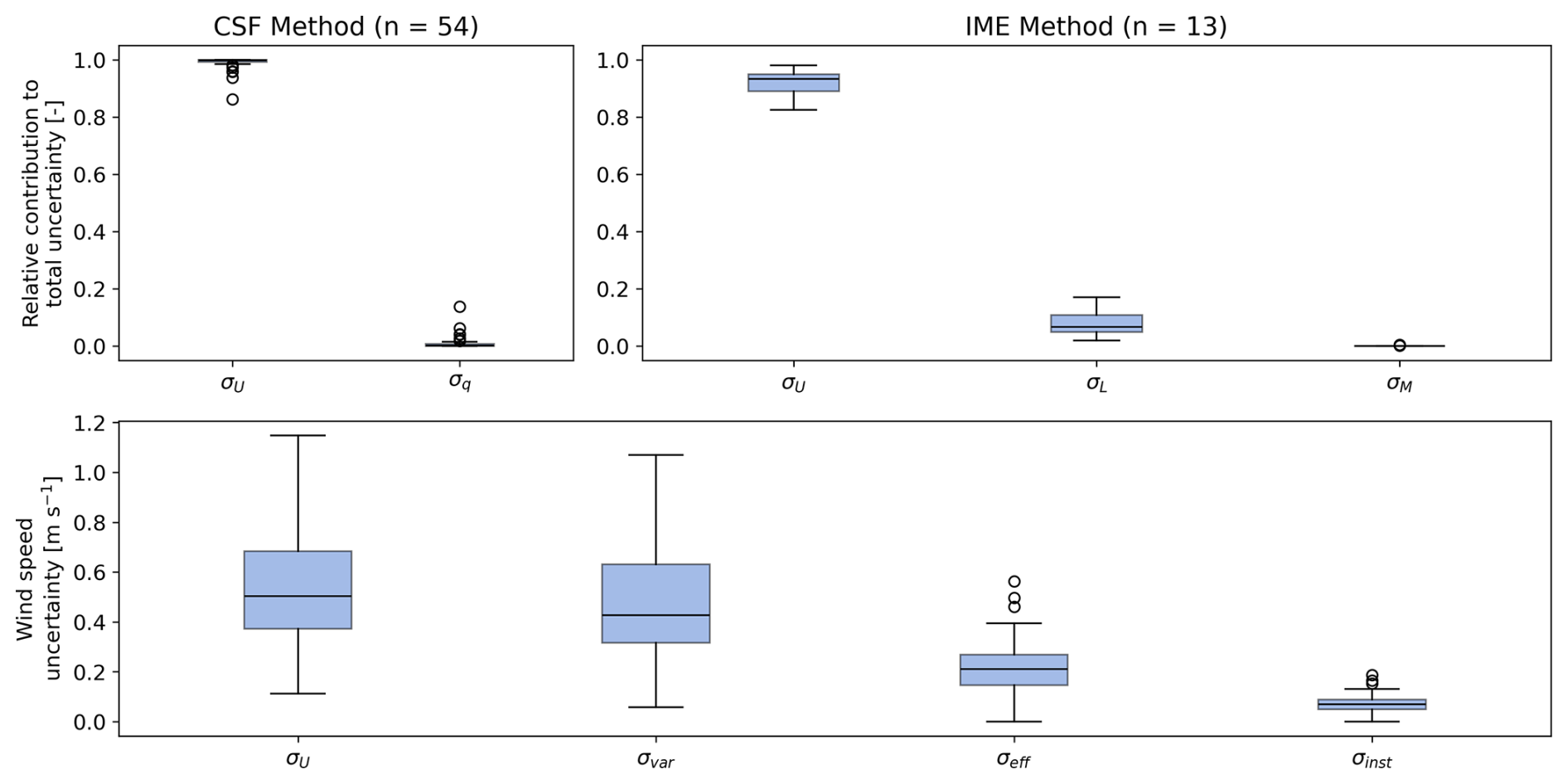
Figure A2 Top row: Relative contribution of the individual uncertainty terms of the CSF and IME to the uncertainty of the estimated emissions Q. Bottom row: wind speed uncertainty contributions by natural variability σ_var, effective wind speed σ_eff and instrument precision σ_inst.

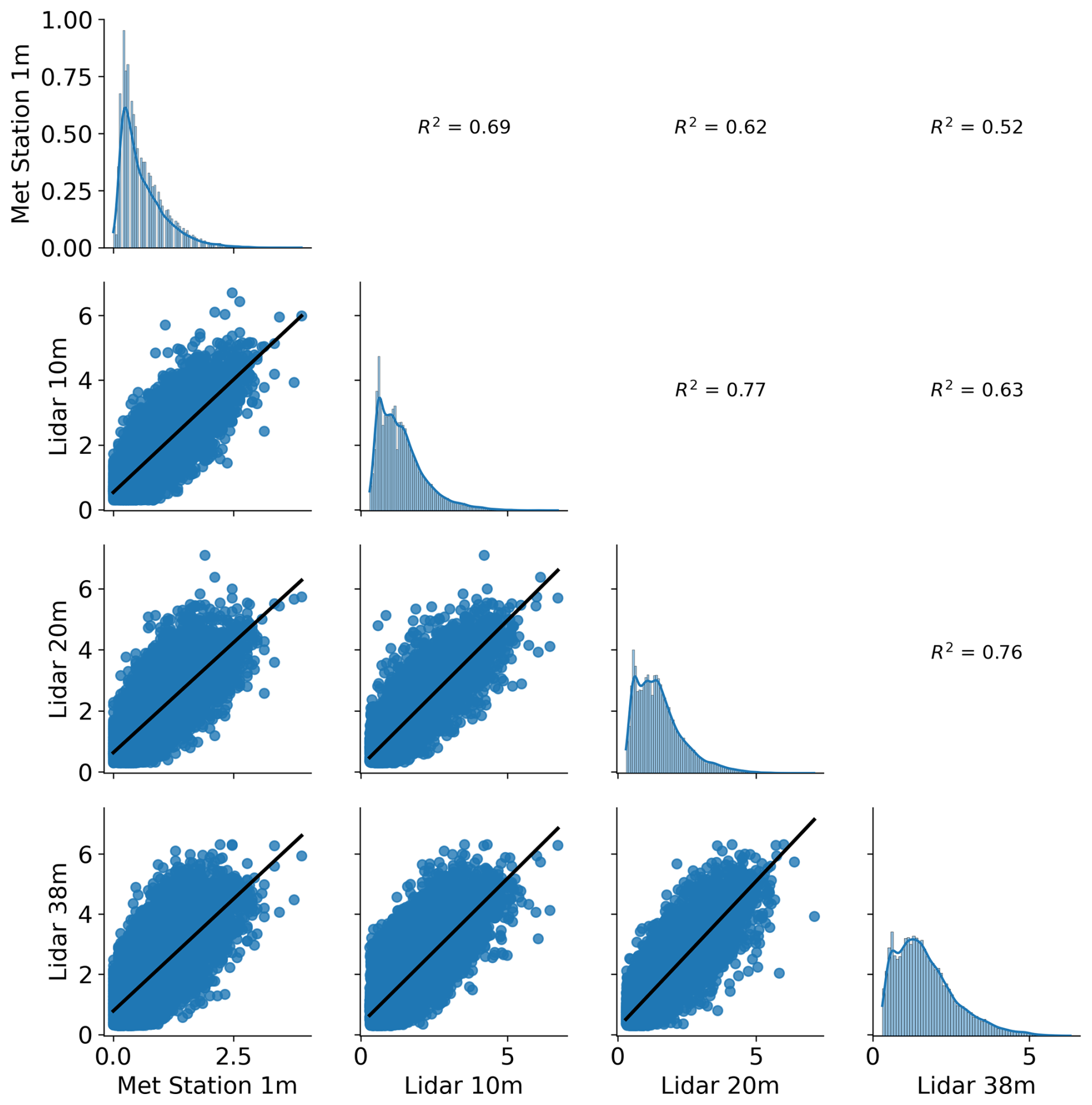
Figure A3 Pair plot of the wind speeds measured by the wind lidar at 10 and 20 m as well as from a meteorological station affixed to the lidar, approximately 1 m off the ground.

Table A1 Average and standard deviation of lidar 10 m wind speed during each release in local time [UTC+2]. Wind data has been resampled to 1 min intervals. NA – not available.

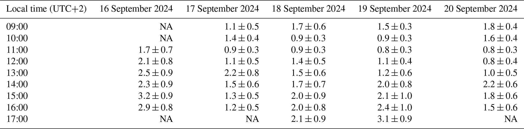
Table A2 Average and standard deviation of lidar 10 m wind direction during each release in local time [UTC+2]. Wind data has been resampled to 1 min intervals. NA – not available.

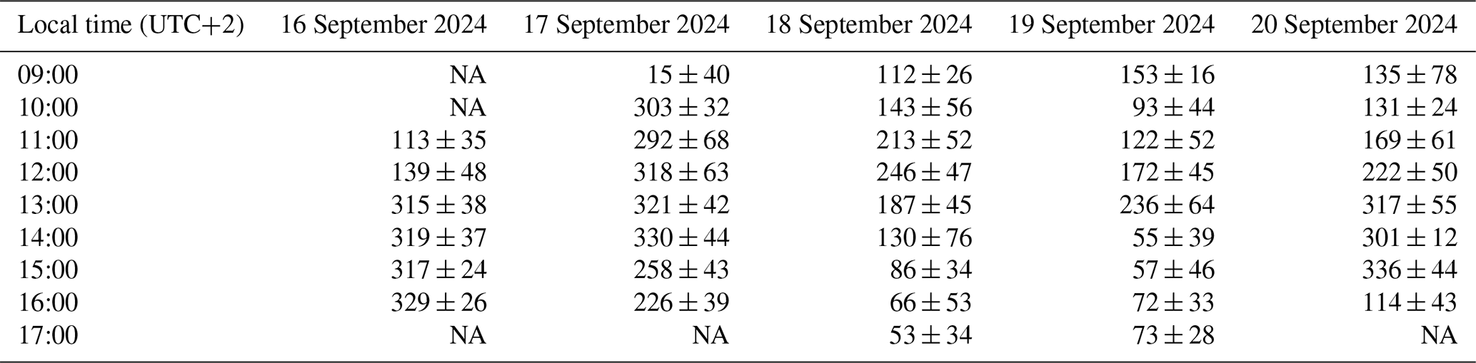
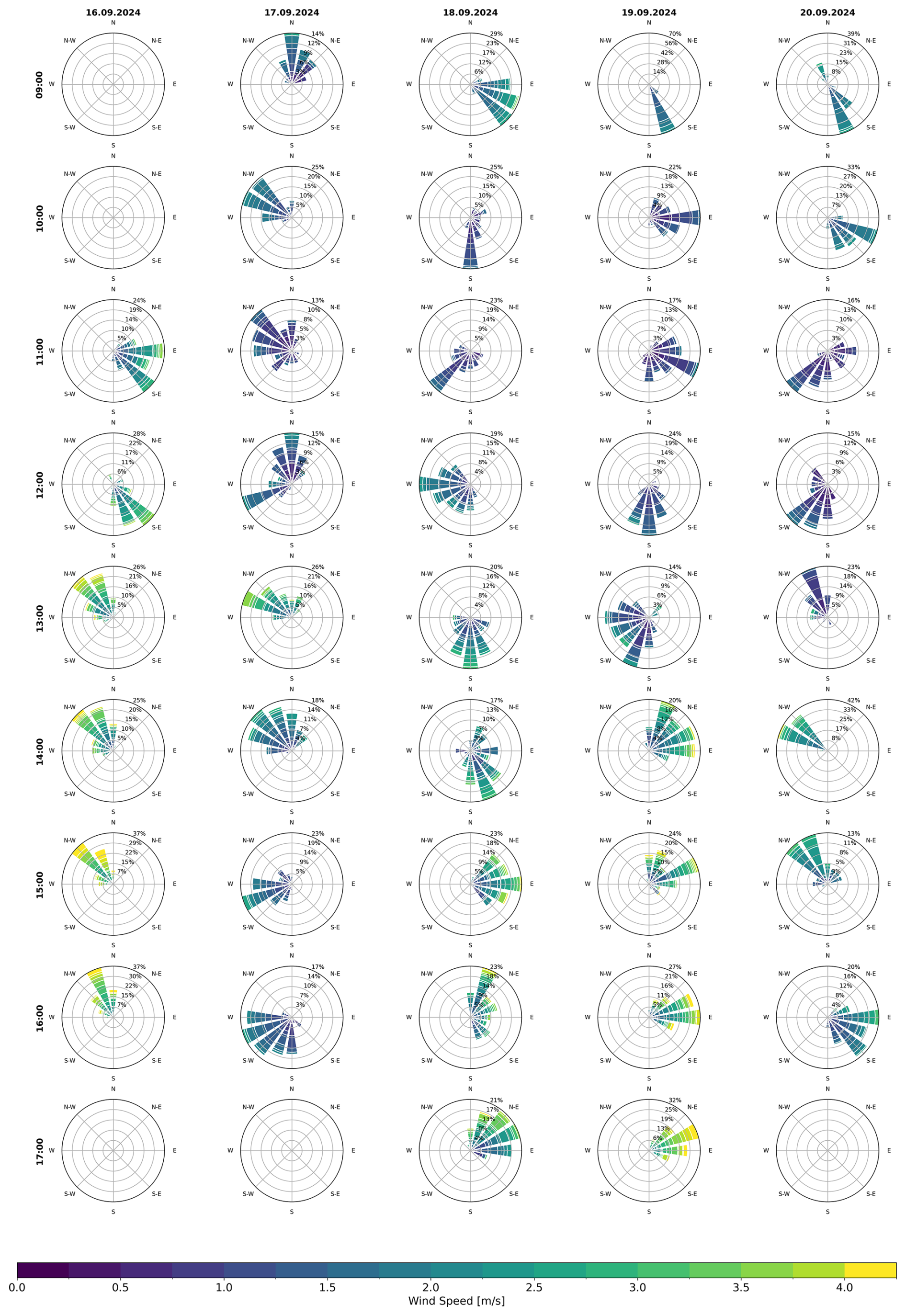
Figure A4 Wind roses of lidar 10 m wind speed and direction during each release in local time [UTC+2].

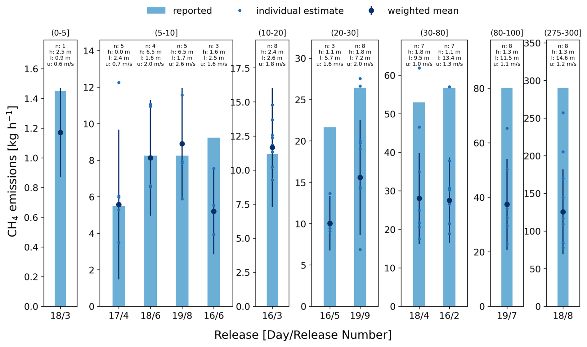
Figure A5 Uncertainty weighted average estimates for each release using U_eff derived in this paper. The number of observations n, emission height h, plume length l and average wind speed u are indicated above each bar.