Calibrating interdependent photochemistry, nucleation, and aerosol microphysics in chamber experiments

Laboratory experiments addressing complex phenomena such as atmospheric new-particle formation and growth typically involve numerous instruments measuring a range of key coupled variables. In addition to independent calibration, the combined dataset provides not just constraints on the parameters of interest but also on the critical instrument calibrations. Here we find good agreement between production and loss rates of sulfuric acid (H₂SO₄) in an experiment performed at the CERN CLOUD chamber involving oxidation of sulfur dioxide (SO₂) in the presence of ammonia (NH₃) at 58 % relative humidity, driving new-particle formation and growth of particles by H₂SO₄+NH₃ nucleation initiated by O₃ photolysis via several light sources. This closure requires consistency across numerous parameters, including: the particle number and size distribution; their condensation sink for H₂SO₄; the particle growth rates; the concentration of H₂SO₄; and the nucleation coefficients for both neutral and ion-induced pathways. Our study shows that accurate agreement can be achieved between production and loss of condensable vapors in laboratory chambers under atmospheric conditions, with accuracy ultimately tied to particle number measurement (i.e. a condensation particle counter). This, in turn implies parameters such as the H₂SO₄ concentration and particle size distributions can be determined to a comparable precision.

1 Introduction

The Cosmics Leaving OUtdoor Droplets (CLOUD) experiment at CERN was designed to determine particle nucleation rates under atmospheric conditions, including the effect of ionization from galactic cosmic rays (Kirkby et al., 2011; Duplissy et al., 2016). Experiments such as this are complex, involving many interconnected measurement and theoretical parameters. These parameters are often constrained separately, for example via offline instrument calibration, characterization of transfer functions, sample line-loss corrections, and so forth. All these calibrations and corrections are subject to random and systematic error.

Some calibrations depend on these other calibrations for their own accuracy. An example central to this paper is actinometry – specifically calibration of actinic fluxes from UV lights driving O₃ photolysis, OH production, SO₂ oxidation and thus H₂SO₄ vapor production. Calibration of light intensities requires accurate measurement of several gas concentrations, including H₂O, O₃, SO₂, all species that react with OH at significant rates, and H₂SO₄ itself. Here we shall consider an even larger set of interconnected measurements with associated signals or values incorporating particle nucleation and subsequent growth governed by that H₂SO₄ vapor. All the values have a priori (independent) calibration parameters (“prm”) for signals, {s_prm}, or other values, {κ_prm}, etc; these include: gas-phase concentrations; particle number; particle charge; size distributions; light spectra, intensities, and amplitudes; and constants such as first-order wall loss, rate coefficients, etc.

Our objective is to scale the a priori parameters by a set of calibration factors, $\mathit{\left\{}{\mathcal{F}}_{\mathrm{prm}}^{\mathrm{cal}}\mathit{\right\}}$, to obtain overall consistency among the various measurements in the combined dataset, constrained by models of gas-phase photochemistry and aerosol microphysics. If all measurements were initially perfect and independent, we would find a solution ${\mathcal{F}}_{\mathrm{prm}}^{\mathrm{cal}}=\mathrm{1}\pm \mathrm{0}$ along a diagonal. Our ultimate aim is to find $\mathit{\left\{}{\mathcal{F}}_{\mathrm{prm}}^{\mathrm{cal}}\mathit{\right\}}$ through a formal optimization and so also obtain a probability density function $\mathit{\left\{}{\mathcal{P}}_{\mathrm{prm}}^{\mathrm{cal}}\mathit{\right\}}$, including a full covariance among all of the factors (Ozon et al., 2021a, b). Those covariances serve formally as the strong interconnections between measurements that can substantially reduce the overall uncertainty.

This work sets the table for that ambitious goal. Here we present a less formal proof-of-concept to obtain “by eye” estimates of the most likely $\mathit{\left\{}{\mathcal{F}}_{\mathrm{prm}}^{\mathrm{cal}}\mathit{\right\}}$. Even this less formal method can substantially tighten constraints on important parameters while building a self consistent representation of the experimental system. We shall argue that the interconnected calibrations are much more robust, and accurate, than any of the individual, a priori, values.

2 Methods

The CERN CLOUD chamber is a 26.1 m³ stainless steel reactor maintained to a high degree of cleanliness. It is fed by ultrapure cryogenic N₂ and O₂ and operated as a continuously stirred tank reactor (CSTR), with inductively coupled mixing fans at the top and bottom maintaining well-mixed conditions (Kirkby et al., 2011; Duplissy et al., 2016). Flow in is balanced by flow out (largely to the many sampling instruments) with a dilution timescale of roughly 1.5 h and pressure maintained slightly above the ambient pressure in Geneva (965 hPa mean) to ensure that no contamination leaks into the chamber. An insulated thermal housing permits operation between 213 and 313 K. Water is added via a nafion™ humidifier to control the relative humidity. Under typical operating conditions with the fans at 12 % of their maximum speed, the resulting turbulent loss of vapors such as H₂SO₄ to the chamber walls proceeds with a first-order time constant of roughly 500 s (Stolzenburg et al., 2020).

The chamber was designed with careful control over ionization conditions and can operate in three modes: neutral, galactic cosmic ray (“gcr”) and beam. In the neutral mode electrodes at the top and bottom of the chamber establish a 20 kV m⁻¹ clearing field to sweep out all primary ions in roughly 1 s (Kirkby et al., 2011). In the gcr mode, the clearing field is off and ion-pair formation governed by incident cosmic rays (along with stray muons from the CERN beam target) forms ion pairs at a rate of 2–7 cm⁻³ s⁻¹. In the beam mode, a 3.5 GeV π⁺ diffuse beam from the CERN proton synchrotron increases the ion-pair formation rate up to 100 ion pairs cm⁻³ s⁻¹, reproducing ion-pair concentrations found in the upper troposphere.

CLOUD is illuminated by multiple different light sources to initiate photolysis of various gases. Three light sources are important here. A set of four Hg−Xe lamps (Hamamatsu) is coupled to the chamber via an array of carefully aligned optical fiber bundles fixed in the top cover of the chamber and oriented to provide relatively homogeneous light intensity (Kupc et al., 2011). These lights are known as “UVH” and can be adjusted via electro-mechanical apertures in each lamp housing. One optical fiber bundle located on the upper access cover at the top of the chamber couples a 248 nm Kr−F excimer laser into the chamber (Lehtipalo et al., 2016). This light is known as “UVX” and can be adjusted by controlling the laser pulse repetition frequency and pulse energy. Finally, a bank of UV light emitting diodes with peak intensities near 385 nm projects radially into the chamber at the middle level, along with the instrument sampling ports, with LEDs pointing axially upwards and downwards in pairs (Lehtipalo et al., 2016). These diodes are housed in a quartz jacket and are cooled with chilled recirculating liquid to remove excess heat, and the 385 nm LED “light saber” is known as LS3. The various light amplitudes are measured with the combination of a UVVis spectrometer and several photodiodes, all of which are coupled to the chamber via optical fibers located on the lower access cover, at the bottom of the chamber (Finkenzeller et al., 2022). The details of that measurement are described in a separate paper, but here the amplitude (signal) of each light appears as s_lt.

2.1 Approach

Multiple instruments are important to this paper, and we follow a sequence motivated by the dependencies illustrated in Fig. 1. The gas and particle phases are largely independent, with the main and critically important interdependency between the H₂SO₄ vapor concentration and the overall particle condensation sink (which can compete with wall loss as an H₂SO₄ sink). The H₂SO₄ governs particle growth rates and, along with NH₃ (and H₂O) the nucleation rates as well, and so controls the condensation sink. With the absolute H₂SO₄ constrained, it is relatively straightforward to propagate backwards (invert) for the photolysis rates and thus calibrate the absolute light intensities.

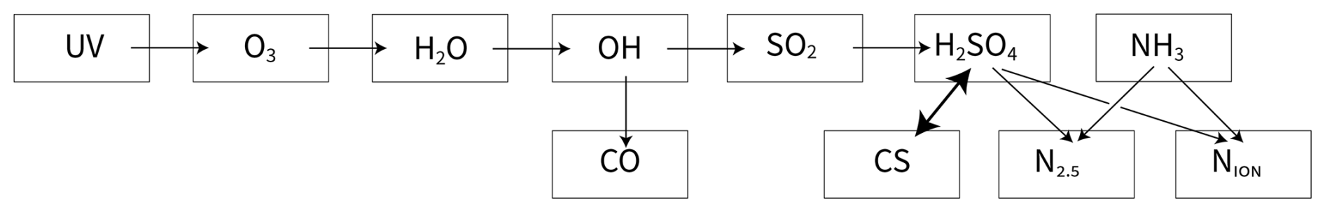
Figure 1 Dependency scheme of interconnected measurements linking UV intensities to new-particle formation, and the elements required for a robust calibration. Gas phase species (and light) drive particle microphysics (nucleation and growth) depicted by the condensation sink (CS) and the total particle number (N_2.5) as well as the ion distribution (N_ion). The ability to measure N_2.5 accurately (with a condensation particle counter) and H₂SO₄ precisely (with an ${\mathrm{NO}}_{\mathrm{3}}^{-}$ chemical ionization mass spectrometer) permits a robust constraint on H₂SO₄ first-order loss as well as absolute calibration, particle growth rates, and the particle nucleation rate. Most importantly, the H₂SO₄ vapor and condensation sink are interdependent, as the number and size of the particles, which determine CS, are both governed by the H₂SO₄ vapor concentration, but CS in turn (can be) a major sink of H₂SO₄. This propagates backwards to the UV light intensities and O₃ photolysis rates.

2.1.1 Gas measurements

Relative humidity (RH) is measured with a commercial RH sensor for dew points above 260 K. Ozone (O₃) is produced in an external generator from pure O₂ irradiated with 185 nm VUV light and measured via UV absorption. There O₃ generation might form some contaminant VOCs, but previous work has shown these to be negligible (Schnitzhofer et al., 2014). Carbon monoxide (CO) is always present in cryogenic N₂ but was not measured at CLOUD during the campaign described here; however, measurements during subsequent campaigns have shown a constant CO concentration of roughly 100 ppbv. There was no methane added to the pure synthetic air mixture, and no added NO_x during the run described here. Sulfur dioxide (SO₂) is added to CLOUD from a compressed gas cylinder via a mass flow controller in the gas handling system and measured with a calibrated SO₂ instrument. Sulfuric acid vapor (H₂SO₄) is measured with two (semi) independently calibrated ${\mathrm{NO}}_{\mathrm{3}}^{-}$ chemical ionization time-of-flight mass spectrometers (there was some post campaign reconciliation). Ammonia (NH₃) is measured with a Picarro PI2103 analyzer, by mass spectrometry at concentrations below 1 ppbv, and also constrained via the steady-state balance between a known flow in and the chamber dilution timescale.

We regard the RH, O₃ and SO₂ measurements as well calibrated and relatively straightforward. Furthermore, the dependencies in Fig. 1 show that inversion from known H₂SO₄ vapor concentrations back to calibrating the intensity of various UV light sources is straightforward; uncertainties in calibration of each measurement (SO₂, CO, H₂O, O₃, etc.) propagate directly in quadrature to uncertainty in the absolute light calibration itself. However, precision in these measurements enables precise constraints and precise model-measurement intercomparison of H₂SO₄ measurements with the model, and once both the loss rate and concentration of H₂SO₄ are constrained accurately, then the production rate of H₂SO₄ is also constrained accurately. Here we are focused on the right-hand side of Fig. 1, combining particle measurements with H₂SO₄ and NH₃. Those H₂SO₄ and NH₃ measurements are more difficult and thus uncertain. All gas-phase instruments are corrected for vapor losses during sampling, but the H₂SO₄ calibration itself depends on a known and controlled production and loss in a custom designed calibrator (Kürten et al., 2012) and NH₃ is notoriously sticky and difficult to correct for surface equilibration and humidity effects, especially at the sub-ppb levels typically used in CLOUD.

2.1.2 Particle measurements

In addition to the gas measurements, several particle instruments are also important. The number concentration of particles with a mobility diameter greater than 2.5 nm is measured with a butanol condensation particle counter, known as the CPC_2.5. The size distribution of particles is measured with an ensemble of instruments; here we rely on a scanning mobility particle sizer (SMPS) for particles larger than 7 nm and on a “DMA train” (Stolzenburg et al., 2017) for particles between 1.5 and 7 nm. Finally, charged particles are measured with two Air Ion Spectrometers (AIS) operating in negative and positive mode, each with a succession of electrodes to measure ions with mobility diameters between 0.9 and 40 nm (the commercial instrument is known as an NAIS (Mirme and Mirme, 2013) because a corona wire can also charge neutral particles for subsequent detection, but that was not used here).

The CPC_2.5 is the cornerstone of this analysis; as an inversion our method works backwards in Fig. 1 toward $P_{{\mathrm{H}}_{\mathrm{2}}{\mathrm{SO}}_{\mathrm{4}}}$ (sulfuric acid vapor production) and ultimately to $j_{\mathrm{O}{(}^{\mathrm{1}}\mathrm{D})}$ (photolysis of ozone to produce O(¹D)) and the calibrated UV light intensity. Especially when most of the particles are larger than 2.5 nm, sample line losses are minimal and the particle sampling efficiency is near 100 %. The other particle measurements are less certain. The SMPS measurements depend on a known charging efficiency in the particle neutralizer and also known transmission within the differential mobility analyzer (DMA) column. We regard the size distribution amplitude measurement as precise, though particle water content and possible drying while sampling and classifying adds uncertainty to the (mobility) size determination itself. The absolute magnitude of the SMPS is less accurate. The DMA train has similar systematic uncertainties. Finally, the AIS measurements are of highly mobile ions and again subject to systematic uncertainty (Mirme and Mirme, 2013).

3 H₂SO₄ Production and Loss

Here we shall consider a CLOUD calibration run designed to constrain OH production from O₃ photolysis by measurement of H₂SO₄, during which particles nucleated via H₂SO₄+NH₃ “ternary” nucleation and grew via co-condensation of H₂SO₄ and NH₃, rate-limited by H₂SO₄ uptake (Vehkamaki and Riipinen, 2012). Far more (and better) than a simple “actinometry” run, which would rely on accurate H₂SO₄ measurements for the light calibrations, the combined photolysis, nucleation, growth and loss run establishes a robust interconnection of many of the measurements central to CLOUD nucleation rate determinations.

As depicted in Fig. 1, we will show that the combination of the CPC_2.5 with the particle sizing (size distribution) instruments provide accurate measurement of both the particle number distribution and particle surface area distribution, which in turn agree with precisely observed H₂SO₄ first-order losses (to particle condensation and the chamber walls). With the evolving particle size distribution (and total number) well constrained, the particle growth rates and nucleation rates are also well constrained. As particle growth is rate-limited by H₂SO₄ condensation (Stolzenburg et al., 2020), this in turn constrains the absolute H₂SO₄ concentrations and thus the ${\mathrm{NO}}_{\mathrm{3}}^{-}$ CIMS calibrations. Finally, with the gas-phase H₂SO₄ known accurately, it is possible to determine, in order, the SO₂ oxidation rate, the OH concentration, the OH loss and thus production rate (in steady state) and, ultimately, the production rate of O(¹D) from O₃ photolysis and thus the volume averaged actinic flux of each light source (averaged over the overlap between the light source and the O₃ action spectrum toward O(¹D)).

To interpret the observations and develop constraints, ℱ, we will employ a gas-phase photochemical model as well as a microphysical model, connecting the two with observed particle size distributions (which affect the H₂SO₄ condensation lifetime) as well as observed H₂SO₄ (which affects all aspects of the particle microphysics). The following processes are involved, more or less in order but forming a closed loop. The terms c_i, P_i and L_i are the concentration, production and loss rates of species i, k_rxn is the rate coefficient for reaction “rxn”, $k_i^{\mathrm{I}}$ is the overall first-order loss coefficient for species i, and j_proc is a (first-order) photolysis coefficient for process “proc”.

As shown in Fig. 1, the sequence of steps that lead to H₂SO₄ production start with ozone photolysis to produce O(¹D) by light source “lt” with amplitude (signal) s_lt and an (unknown) calibration factor a_lt:

$$\begin{array}{c}{\displaystyle }{j}_{\mathrm{O}{(}^{\mathrm{1}}\mathrm{D})}=a_{\mathrm{lt}}{s}_{\mathrm{lt}}\\ {\displaystyle }{P}_{\mathrm{O}{(}^{\mathrm{1}}\mathrm{D})}=j_{\mathrm{O}{(}^{\mathrm{1}}\mathrm{D})}{c}_{{\mathrm{O}}_{\mathrm{3}}}\\ {\displaystyle }{L}_{\mathrm{O}{(}^{\mathrm{1}}\mathrm{D})}=\left(k_{{\mathrm{N}}_{\mathrm{2}}}{c}_{{\mathrm{N}}_{\mathrm{2}}}+k_{{\mathrm{O}}_{\mathrm{2}}}{c}_{{\mathrm{O}}_{\mathrm{2}}}+k_{{\mathrm{H}}_{\mathrm{2}}\mathrm{O}}{c}_{{\mathrm{H}}_{\mathrm{2}}\mathrm{O}}\right)c_{\mathrm{O}{(}^{\mathrm{1}}\mathrm{D})}^{\mathrm{ss}}\\ {\displaystyle }{P}_{\mathrm{OH}}=\mathrm{2}{k}_{{\mathrm{H}}_{\mathrm{2}}\mathrm{O}}{c}_{{\mathrm{H}}_{\mathrm{2}}\mathrm{O}}{c}_{\mathrm{O}{(}^{\mathrm{1}}\mathrm{D})}^{\mathrm{ss}}+\mathrm{\dots }\\ {\displaystyle }{L}_{\mathrm{OH}}=\left(k_{\mathrm{CO}}{c}_{\mathrm{CO}}+k_{{\mathrm{O}}_{\mathrm{3}}}{c}_{{\mathrm{O}}_{\mathrm{3}}}+k_{{\mathrm{SO}}_{\mathrm{2}}}{c}_{{\mathrm{SO}}_{\mathrm{2}}}+\mathrm{\dots }\right)c_{\mathrm{OH}}^{\mathrm{ss}}\\ {\displaystyle }{P}_{{\mathrm{H}}_{\mathrm{2}}{\mathrm{SO}}_{\mathrm{4}}}=k_{{\mathrm{SO}}_{\mathrm{2}}}{c}_{{\mathrm{SO}}_{\mathrm{2}}}{c}_{\mathrm{OH}}^{\mathrm{ss}}\end{array}$$

This will be balanced by H₂SO₄ loss on a timescale given by the inverse of the overall first-order loss coefficient $k_{{\mathrm{H}}_{\mathrm{2}}{\mathrm{SO}}_{\mathrm{4}}}^{\mathrm{I}}$, which includes terms for wall loss, condensation loss, and ventilation, among others:

$$\begin{array}{c}{\displaystyle }{L}_{{\mathrm{H}}_{\mathrm{2}}{\mathrm{SO}}_{\mathrm{4}}}=k_{{\mathrm{H}}_{\mathrm{2}}{\mathrm{SO}}_{\mathrm{4}}}^{\mathrm{I}}{c}_{{\mathrm{H}}_{\mathrm{2}}{\mathrm{SO}}_{\mathrm{4}}}\\ {\displaystyle }{k}_{{\mathrm{H}}_{\mathrm{2}}{\mathrm{SO}}_{\mathrm{4}}}^{\mathrm{I}}=k_{\mathrm{wall}}^{\mathrm{I}}+k_{\mathrm{cond}}^{\mathrm{I}}+\mathrm{\dots }\end{array}$$

The production and loss balance can be used to constrain the calibration factor a_lt, provided that $k_{{\mathrm{H}}_{\mathrm{2}}{\mathrm{SO}}_{\mathrm{4}}}^{\mathrm{I}}$ and $c_{{\mathrm{H}}_{\mathrm{2}}{\mathrm{SO}}_{\mathrm{4}}}$ are known accurately (along with the other concentrations connecting the light intensity to H₂SO₄). However, part of the H₂SO₄ loss is to particles, which in turn form and grow because of H₂SO₄ condensation (the two-way interdependency in Fig. 1). Particle production (J), growth (G), and loss (L) vs. diameter d_p are thus also coupled to this system. These also depend on the particle charge state, which for these tiny particles is either neutral, ∘, or a single positive or negative charge, ±:

$$J_{\mathrm{nuc}}^{\circ ,\pm }=k_{\mathrm{nuc}}^{\circ ,\pm }{c}_{{\mathrm{H}}_{\mathrm{2}}{\mathrm{SO}}_{\mathrm{4}}}^{\mathrm{3}}{c}_{{\mathrm{NH}}_{\mathrm{3}}}{n}^{\circ ,\pm }(n^{\circ }\equiv \mathrm{1})$$

$$\begin{array}{c}{\displaystyle }G\left(d_{\mathrm{p}}\right)=k_{\mathrm{gr}}{c}_{{\mathrm{H}}_{\mathrm{2}}{\mathrm{SO}}_{\mathrm{4}}}\\ {\displaystyle }L\left(d_{\mathrm{p}}\right)=\left(k_{\mathrm{wall}}^{\mathrm{I}}\left(d_{\mathrm{p}}\right)+k_{\mathrm{vent}}^{\mathrm{I}}\right)n\left(d_{\mathrm{p}}\right)\end{array}$$

Finally, the production of primary ions, n^± is given by an ion-pair formation rate Q_ip (by cosmic rays or the CERN pion beam) while the loss of those primary ions includes wall loss, ion recombination, ion-induced nucleation, and diffusion charging and neutralization of larger particles, ${\mathcal{C}}^{\circ ,\pm }$:

$$\begin{array}{c}{\displaystyle }{P}_{\pm }=Q_{\mathrm{ip}}\\ {\displaystyle }{L}_{\pm }=\left(k_{\mathrm{wall}}^{\mathrm{I}}+k_{\mathrm{ion}}{n}^{\mp }\right)n^{\pm }+J_{\mathrm{nuc}}^{\pm }+{\mathcal{C}}^{\circ ,\mp }\end{array}$$

As a test case we consider an actinometry run during the CLOUD11 campaign in Autumn 2016. Run 1833 lasted from roughly 17:30 CET on 31 October to roughly 04:00 CET on 2 November, with the chamber at 297.8 K, 58 % relative humidity, and 987 hPa. O₃ was near 42 ppbv, SO₂ near 2 ppbv, NH₃ at 2 ppbv, and CO was near 100 ppbv.

Raw measurements

We show data from Run 1833 in Figs. 2–4. The run comprised a sequence of 26 stages, each with different nominal conditions. The stages are marked in the figures by dashed vertical gray lines numbered at the top. During intervals comprising sets of stages, we systematically increased the amplitudes of different light sources (principally UVH and UVX) with pairs of neutral and charged (gcr) stages, and we followed each interval with a “cleaning” stage to remove particles from the chamber.

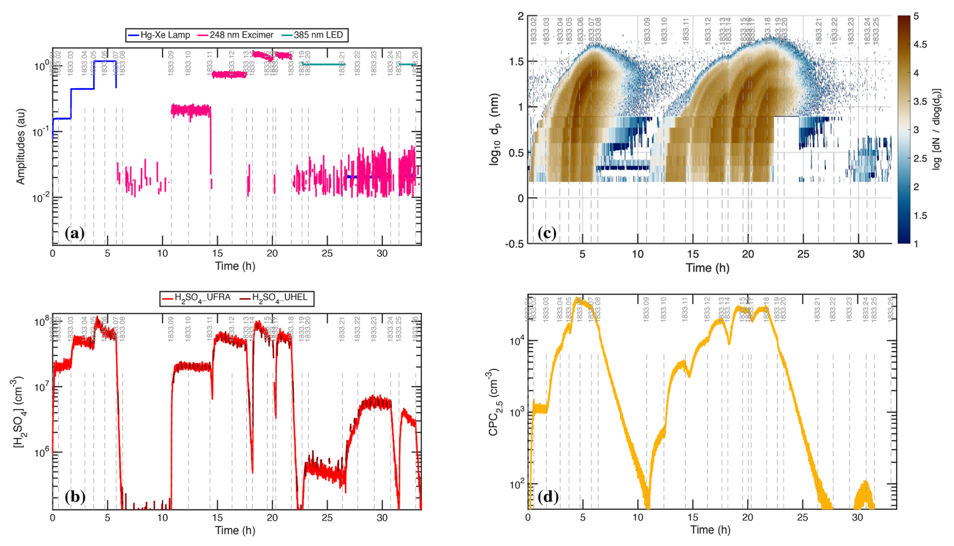
Figure 2 Raw photochemical observations vs. time for CLOUD11 Run 1833. Individual run stages are demarcated by dashed vertical gray lines, with the stage number at the top (i.e. 1833.09 at hour 11). (a) Light amplitudes obtained from a UVVis spectrometer vs. time (UTC). The run included two intervals with systematic amplitude steps for a single light source: first the “UVH stages” (stages 01–08 with steps in the dark blue Hg−Xe lamp, known as UVH) and second the “UVX stages” (stages 09–18 with steps in the magenta Excimer laser, known as UVX). (b) H₂SO₄ measured by two ${\mathrm{NO}}_{\mathrm{3}}^{-}$ CIMS. The lighter red values are from a dedicated H₂SO₄ instrument whereas the darker red values are from a “HO_x−RO_x” instrument with a modified inlet alternating between H₂SO₄ mode and HO_x mode. During the UVH and UVX stages, the H₂SO₄ signal follows the steps in light intensity as seen in panel (a), with important deviations. (c) Particle size distribution obtained by merging data from the DMA train, a nano-SMPS and an SMPS. The DMA train covers $\mathrm{1.7}<d_{\mathrm{p}}<\mathrm{7.9}$ nm with lower size resolution but greater accuracy than the SMPS. Both the UVH and UVX sub-runs display nucleation bursts associated with each stage, forming “bunches of bananas” with near monotonically increasing CPC_2.5 concentrations. Data from the DMA train are missing near run time 22–24 h. (d) Total particle number above 2.5 nm mobility diameter measured with a Condensation Particle Counter (CPC_2.5).

Figure 2a shows the unfiltered amplitudes of the three light sources over the course of the run, obtained from the UVVis spectrometer, including some crosstalk. The light sources are labeled in the figure as “Hg−Xe lamp” (UVH), “248 nm excimer laser” (UVX), and “385 nm LED” (LS3). During the run, first the Hg−Xe lamps (stages 01–08; the UVH stages) and then the excimer laser (stages 09–18; the UVX stages) were systematically stepped through 3 intensities, at roughly 10 %, 40 % and 100 % of full power. After this the 385 nm LEDs were turned on at full power (stages 19 and 20) and finally all the lights were turned on in sequence (stages 21–26), with the Hg−Xe and excimer lights at low power and the LEDs again at full power. With every change of light intensity, the H₂SO₄ shown in Fig. 2b changed rapidly in response, for the most part reaching a steady state within minutes, reflecting the wall-loss timescale of H₂SO₄. However, while the H₂SO₄ broadly followed the steps in light amplitudes, there are obvious deviations, notably when the H₂SO₄ concentration was high during stages 05–06 and again during stages 14–15.

The H₂SO₄ depletion below the expected values at the highest light intensities was caused by (progressively increasing) condensation to particles. Especially during the UVH and UVX stages, the H₂SO₄ concentration was high enough to drive nucleation and substantial growth, which in turn built up a condensation sink competitive with wall loss for condensable vapors such as H₂SO₄. Figure 2c shows particle size distributions vs. time, measured with a scanning mobility particle sizer (SMPS), a nano-SMPS, and a DMA train. This shows a succession of overlapping nucleation and growth bursts (a bunch of bananas) while the Hg−Xe and excimer light sources were being stepped up. Here we use physical particle diameter (d_p) to represent (and model) the size distribution but retain the standard practice of describing classifiers by their classification size (here mobility diameter, d_mob); we relate the two with $d_{\mathrm{mob}}=d_{\mathrm{p}}+\mathrm{0.3}$ nm (Larriba et al., 2011). Figure 2d shows the total particle number above 2.5 nm (mobility diameter) measured with a condensation particle counter (CPC_2.5).

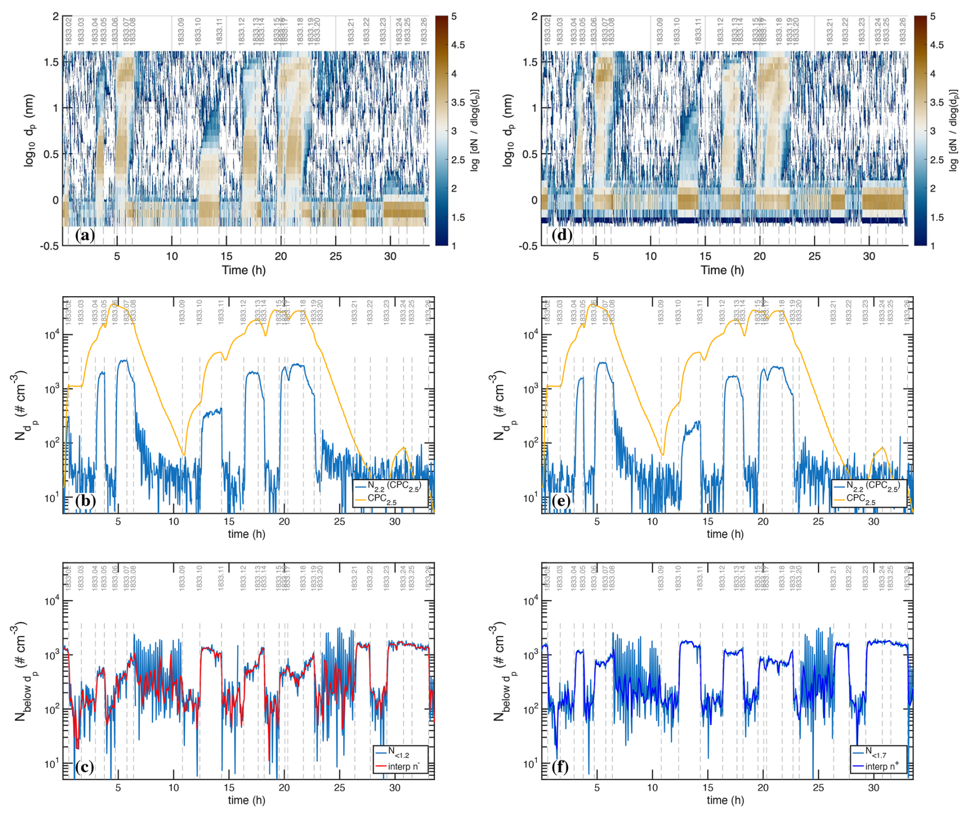
Figure 3 Negatively (a–c) and positively (d–f) charged particle observations before background correction, compared with total (neutral + charged) particle counts. (a, d) Air Ion Spectrometer (AIS) distributions; (b, e) total AIS number for given polarity above 2.2 nm (2.5 nm mobility diameter) compared with total CPC_2.5; (c, f) charged particle number smaller than 1.2 nm (left, negatively charged) and 1.7 nm (right, positively charged), constituting the primary ions, along with a filtered interpolant. Strong ion-induced nucleation stages (i.e. 06, 17) show nearly equal negatively and positively charged particles near 3×10³ cm⁻³ comprising, in total, roughly 20 % of the total CPC_2.5 concentration. During weak ion-induced nucleation (i.e. stage 10) the negatively charged particles are roughly twice as abundant as the positively charged particles (300 vs. 150 cm⁻³). The level signal of small ions in the bottom panels of ∼200 cm⁻³ during neutral stages (with a high-voltage clearing field turned on) are due to instrumental electronic noise; the true ion concentrations are well below 10 cm⁻³. The oscillating signals during cleaning stages 08 and 20 are caused by alternating on/off cycles of the high-voltage clearing field.

Figure 3 shows charged particle size distributions from the two air-ion spectrometers (AIS), one in negative mode (Fig. 3a–c, left panels) and one in positive mode (Fig. 3d–f, right panels). The top panels (Fig. 3a and d) are the measured size distributions, the middle panels (Fig. 3b and e) are the integrated cuts above d_p=2.2 nm (compared with the total CPC_2.5 measurement of all particles), and the bottom panels (Fig. 3c and f) are integrated counts below a cut size of 1.2 nm for the negative particles and 1.7 nm for the positive particles, along with a median filtered interpolant of these values. These small particles are the primary ions responsible for ion-induced nucleation.

For the UVH and UVX stages, each light power setting included a neutral stage (field on) and a stage charged by galactic cosmic rays (gcr, field off). In most cases the neutral stage preceded the charged stage so that the weaker neutral nucleation could be easily distinguished from stronger ion-induced nucleation. An exception is the first pair of stages, 01 and 02, where the chamber was initially charged in stage 01 and then switched to neutral in stage 02. This was because neutral nucleation under these low H₂SO₄ conditions is very weak, and the initial burst of ion-induced nucleation during stage 01 appears as a clear mode growing toward 20 nm over time in Fig. 2c. For all the other pairs at a fixed light setting during both the UVH and UVX stages, the neutral stage preceded the charged stage.

The run included two cleaning stages (08 and 20), during which the clearing field alternated between on and off with the pion beam also on. During these stages the AIS data oscillate between the highest and very low values, which is clearly evident in the raw particle number counts (Fig. 3c and f). These cleaning stages are designed to generate primary ions with the clearing field off, which then charge a fraction of the larger particles via diffusion charging. When the clearing field turns on, these charged particles are then swept out of the chamber. Because the steady state charged fraction of these small particles is very low (as is clearly evident in the middle panels of these figures), this alternating method first removes any charge particles and then builds the charge distribution back towards the steady state value, thus progressively removing the larger particles (which would otherwise be removed on the slow ventilation timescale of the chamber).

Because the condensation sink occasionally grew to be competitive with wall loss, we must account for this to quantitatively constrain H₂SO₄ production and loss. However, the evident exponential drop in H₂SO₄ in, e.g., stages 05–06 shows that the enhanced H₂SO₄ loss is also a measurement of the condensation sink; this is a first-order term requiring only precise H₂SO₄ measurements, not accurate knowledge of the H₂SO₄ absolute calibration. Further, the growth (rate) of the particles was governed by H₂SO₄ condensation; consequently, with the condensation sink well constrained, the growth rate in turn constrains the absolute H₂SO₄ concentration, provided we can account for the role of co-condensing NH₃ and H₂O. Finally, the nucleation rates (neutral and charged) also depend strongly on the H₂SO₄ concentration (in addition to NH₃ and ion concentrations) and so with all these other parameters fixed by multiple constraints, the concentrations driving observed nucleation rates are known accurately.

We show two other important gas-phase measurements in Fig. 4: (a) O₃ and (b) SO₂. Ozone photolysis leading to OH drives the whole system, H₂SO₄ is produced via SO₂+OH, and so the production rate is proportional to both of these. Both O₃ and SO₂ include notable variations, which we will discuss below. In addition to those, the absolute H₂O was known because T and RH were controlled, whereas the gas-phase NH₃ measurement was unreliable and CO (present in synthetic air) was unmeasured. Both were likely constant during Run 1833 but affect some of the absolute calibrations.

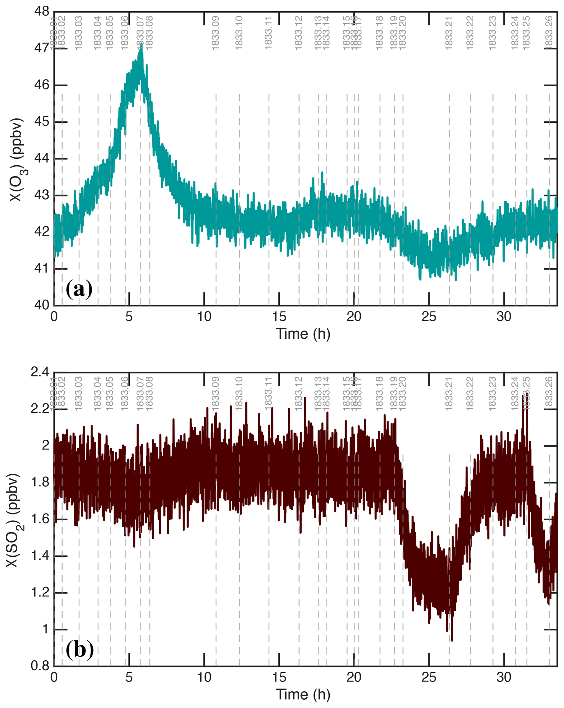
Figure 4 Chemical drivers for H₂SO₄ formation without median filtering. (a) O₃ mixing ratio. (b) SO₂ mixing ratio. Increased O₃ during stages 1–6 is caused by O₂ photolysis by the Hg−Xe arc lamps. Nearly stoichiometric (1 : 1) depletion of SO₂ and O₃ during stages 19 and 20 (with intense irradiation by 385 nm light) is consistent with photo-enhanced wall uptake of SO₂, presumably leaving SO₄ on the chamber walls.

All the data in Figs. 2 and 4 require some amount of data conditioning. In addition to possible calibration factors, ℱ, most benefit from smoothing. We favor median filters as they exclude outliers and maintain step changes (i.e. lights turning on and off). In many cases we combine median filtering with interpolation to develop interpolants so that we can use the observed data to drive constrained models of gas-phase chemistry and particle microphysics.

The CPC_2.5 particle number concentration is the most robust and accurate measurement in this dataset. Much of the time, most of the particles were between 10 and 30 nm. Particles in this size range have relatively low mobility (compared to molecules). Figure 3 shows they were for the most part neutral. Consequently, line losses between the chamber and the CPC were low. Also, during this run it took many minutes for nucleated particles to grow to this size, whereas the mixing time is of order 1 min, so the CPC_2.5 concentration was nearly homogeneous in the chamber. Finally, the CPC itself is a robust instrument, relying only on activation by a controlled supersaturation of 1-butanol; while there is some particle composition dependence to this activation, that is important only for particles near the cutoff activation diameter (2.5 nm); the particles in these experiments were usually much larger than that cutoff size and so this has a minimal effect. Here we assume detection by the CPC_2.5 is a step-function cut in the size distribution at a physical diameter d_p≥2.2 nm. Overall, we estimate that we constrain N_2.2 with an accuracy of well below 10 % under these conditions.

4 Calibration Elements

To constrain calibration factors, ℱ^cal, our strategy is to start with observational constraints based on instrument precision and then to add in constraints based on accuracy, starting with the CPC_2.5. We shall start with the H₂SO₄ first-order loss terms (wall and condensation), which depend on precise H₂SO₄ signals but not accurate calibration; then we will address particle formation and growth, which both depend on accurate (calibrated) H₂SO₄ measurements; and finally, we will turn to photochemical and microphysical to model H₂SO₄ production, evolution of the particle size distribution, and particle charging. The models will also permit a detailed examination of key process rates.

The absolute H₂SO₄ concentration includes a calibration scaling factor:

$$c_{{\mathrm{H}}_{\mathrm{2}}{\mathrm{SO}}_{\mathrm{4}}}={\mathcal{F}}_{{\mathrm{H}}_{\mathrm{2}}{\mathrm{SO}}_{\mathrm{4}}}^{\mathrm{cal}}{s}_{{\mathrm{H}}_{\mathrm{2}}{\mathrm{SO}}_{\mathrm{4}}}$$

This is the nominal H₂SO₄ concentration (signal) as measured via ${\mathrm{NO}}_{\mathrm{3}}^{-}$ CIMS, $s_{{\mathrm{H}}_{\mathrm{2}}{\mathrm{SO}}_{\mathrm{4}}}$, multiplied by a calibration factor ${\mathcal{F}}_{{\mathrm{H}}_{\mathrm{2}}{\mathrm{SO}}_{\mathrm{4}}}^{\mathrm{cal}}$ based on additional constraints from this unified calibration. In some circumstances there may be “hidden” sulfuric acid contributing to nucleation or growth (Rondo et al., 2016), but this has been shown to be negligible for the (NH₄)₂−SO₄ system (Stolzenburg et al., 2020), and our observations support this finding.

Accurate measurement of H₂SO₄ is so central to nucleation and growth experiments that establishing the best possible ${\mathcal{F}}_{{\mathrm{H}}_{\mathrm{2}}{\mathrm{SO}}_{\mathrm{4}}}^{\mathrm{cal}}$ is in many ways our ultimate objective. This extends even beyond particle formation involving H₂SO₄, because often the calibration of other constituents (i.e. Highly Oxygenated Organic Molecules, HOMs) is also tied to the H₂SO₄ calibration in a chemical ionization mass spectrometer (Ehn et al., 2014).

The central feature of these actinometry runs is the balance of production and loss for H₂SO₄:

$${\displaystyle \frac{\mathrm{d}}{\mathrm{d}t}}{c}_{{\mathrm{H}}_{\mathrm{2}}{\mathrm{SO}}_{\mathrm{4}}}=P_{{\mathrm{H}}_{\mathrm{2}}{\mathrm{SO}}_{\mathrm{4}}}-k_{{\mathrm{H}}_{\mathrm{2}}{\mathrm{SO}}_{\mathrm{4}}}^{\mathrm{I}}{c}_{{\mathrm{H}}_{\mathrm{2}}{\mathrm{SO}}_{\mathrm{4}}}$$

This has a steady-state solution

$$c_{{\mathrm{H}}_{\mathrm{2}}{\mathrm{SO}}_{\mathrm{4}}}^{\mathrm{ss}}={\displaystyle \frac{P_{{\mathrm{H}}_{\mathrm{2}}{\mathrm{SO}}_{\mathrm{4}}}}{k_{{\mathrm{H}}_{\mathrm{2}}{\mathrm{SO}}_{\mathrm{4}}}^{\mathrm{I}}}}=P_{{\mathrm{H}}_{\mathrm{2}}{\mathrm{SO}}_{\mathrm{4}}}{\mathit{\tau }}_{{\mathrm{H}}_{\mathrm{2}}{\mathrm{SO}}_{\mathrm{4}}}$$

If the H₂SO₄ concentration in Fig. 2 is accurately calibrated, then this becomes a constraint on the H₂SO₄ production rate

$$P_{{\mathrm{H}}_{\mathrm{2}}{\mathrm{SO}}_{\mathrm{4}}}=c_{{\mathrm{H}}_{\mathrm{2}}{\mathrm{SO}}_{\mathrm{4}}}^{\mathrm{ss}}{k}_{{\mathrm{H}}_{\mathrm{2}}{\mathrm{SO}}_{\mathrm{4}}}^{\mathrm{I}}={\mathcal{F}}_{{\mathrm{H}}_{\mathrm{2}}{\mathrm{SO}}_{\mathrm{4}}}^{\mathrm{cal}}{s}_{{\mathrm{H}}_{\mathrm{2}}{\mathrm{SO}}_{\mathrm{4}}}^{\mathrm{ss}}{k}_{{\mathrm{H}}_{\mathrm{2}}{\mathrm{SO}}_{\mathrm{4}}}^{\mathrm{I}}$$

Regardless, the light calibration unavoidably involves accurate knowledge of the H₂SO₄ concentration and lifetime; consequently, it is the production rate of H₂SO₄ that is most directly calibrated.

4.1 Loss constraints

When $P_{{\mathrm{H}}_{\mathrm{2}}{\mathrm{SO}}_{\mathrm{4}}}\ll k_{{\mathrm{H}}_{\mathrm{2}}{\mathrm{SO}}_{\mathrm{4}}}^{\mathrm{I}}{c}_{{\mathrm{H}}_{\mathrm{2}}{\mathrm{SO}}_{\mathrm{4}}}$ (as in stages 07–08, 13, and 18), the H₂SO₄ follows pseudo first-order loss

$${\displaystyle \frac{\mathrm{d}}{\mathrm{d}t}}\ln \left(s_{{\mathrm{H}}_{\mathrm{2}}{\mathrm{SO}}_{\mathrm{4}}}\right)\simeq -k_{{\mathrm{H}}_{\mathrm{2}}{\mathrm{SO}}_{\mathrm{4}}}^{\mathrm{I}}$$

That first-order sulfuric acid loss (inverse lifetime) comprises several elements

$$\begin{array}{rl}{k}_{{\mathrm{H}}_{\mathrm{2}}{\mathrm{SO}}_{\mathrm{4}}}^{\mathrm{I}}& =k_{{\mathrm{H}}_{\mathrm{2}}{\mathrm{SO}}_{\mathrm{4}}}^{\mathrm{wall}}+k_{{\mathrm{H}}_{\mathrm{2}}{\mathrm{SO}}_{\mathrm{4}}}^{\mathrm{cond}}+\left(k_{{\mathrm{H}}_{\mathrm{2}}{\mathrm{SO}}_{\mathrm{4}}}^{\mathrm{dil}}+k_{{\mathrm{H}}_{\mathrm{2}}{\mathrm{SO}}_{\mathrm{4}}}^{\mathrm{nuc}}+\mathrm{\dots }\right)\\ & ={\mathcal{F}}_{{\mathrm{H}}_{\mathrm{2}}{\mathrm{SO}}_{\mathrm{4}}}^{\mathrm{wall}}{\mathit{\kappa }}_{{\mathrm{H}}_{\mathrm{2}}{\mathrm{SO}}_{\mathrm{4}}}^{\mathrm{wall}}+{\mathcal{F}}_{{\mathrm{H}}_{\mathrm{2}}{\mathrm{SO}}_{\mathrm{4}}}^{\mathrm{cond}}{\mathit{\kappa }}_{{\mathrm{H}}_{\mathrm{2}}{\mathrm{SO}}_{\mathrm{4}}}^{\mathrm{cond}}+\mathrm{\dots }\end{array}$$

We expect loss to be dominated by wall loss and condensation, but it also includes dilution by flow into and out of the chamber and, potentially, nucleation (or formation of “hidden sulfuric acid” clusters that are not well measured by the ${\mathrm{NO}}_{\mathrm{3}}^{-}$ CIMS; Rondo et al., 2016).

It is crucial for the calibration experiments to include stages that are almost completely governed by wall loss as well as others where condensation loss is competitive with or even greater than wall loss. This variability and dynamic range robustly disentangles these two crucial parameters and permits accurate determination of both via precise H₂SO₄ measurements.

4.2 Production constraints

The H₂SO₄ production rate is nominally proportional to the UV light amplitudes, s_lt, but the absolute magnitude also depends on the H₂SO₄ calibration:

$$\begin{array}{c}{\displaystyle }{p}_{{\mathrm{H}}_{\mathrm{2}}{\mathrm{SO}}_{\mathrm{4}}}=y_{{\mathrm{H}}_{\mathrm{2}}{\mathrm{SO}}_{\mathrm{4}}}\left(c_{{\mathrm{SO}}_{\mathrm{2}}},c_{\mathrm{CO}},c_{{\mathrm{H}}_{\mathrm{2}}\mathrm{O}},c_{{\mathrm{O}}_{\mathrm{3}}}\right){\mathcal{L}}_{\mathrm{lt}}^{\mathrm{cal}}{s}_{\mathrm{lt}}\\ {\displaystyle }{P}_{{\mathrm{H}}_{\mathrm{2}}{\mathrm{SO}}_{\mathrm{4}}}={\mathcal{F}}_{{\mathrm{H}}_{\mathrm{2}}{\mathrm{SO}}_{\mathrm{4}}}^{\mathrm{cal}}{\mathcal{F}}_{\mathrm{lt}}^{\mathrm{cal}}{p}_{{\mathrm{H}}_{\mathrm{2}}{\mathrm{SO}}_{\mathrm{4}}}\end{array}$$

We break the production into a nominal production rate, $p_{{\mathrm{H}}_{\mathrm{2}}{\mathrm{SO}}_{\mathrm{4}}}$, and the fully calibrated value $P_{{\mathrm{H}}_{\mathrm{2}}{\mathrm{SO}}_{\mathrm{4}}}$, which is scaled by the same H₂SO₄ calibration factor, ${\mathcal{F}}_{{\mathrm{H}}_{\mathrm{2}}{\mathrm{SO}}_{\mathrm{4}}}^{\mathrm{cal}}$ along with a slight adjustment for each light calibration, ${\mathcal{F}}_{\mathrm{lt}}^{\mathrm{cal}}$, reflecting any non-linearities propagating through the system with changes to the absolute H₂SO₄ levels. However, at this point in the process, the main feature is that we expect H₂SO₄ production to be proportional to the light amplitudes, scaled by an action term for each light, ${\mathcal{L}}_{\mathrm{lt}}^{\mathrm{cal}}$ (giving the photolysis rate of ${\mathrm{O}}_{\mathrm{3}}⟶{\mathrm{O}}_{\mathrm{2}}+\mathrm{O}{(}^{\mathrm{1}}\mathrm{D})$ at unit light amplitude) and a yield of H₂SO₄ per O(¹D) formed, $y_{{\mathrm{H}}_{\mathrm{2}}{\mathrm{SO}}_{\mathrm{4}}}$, which is a function of several concentrations as well. In practice that function is a photochemical model. The steady-state balance gives

$$\begin{array}{c}{\displaystyle }{P}_{{\mathrm{H}}_{\mathrm{2}}{\mathrm{SO}}_{\mathrm{4}}}=L_{{\mathrm{H}}_{\mathrm{2}}{\mathrm{SO}}_{\mathrm{4}}}\\ {\displaystyle }{\mathcal{F}}_{\mathrm{lt}}^{\mathrm{cal}}{p}_{{\mathrm{H}}_{\mathrm{2}}{\mathrm{SO}}_{\mathrm{4}}}{y}_{{\mathrm{H}}_{\mathrm{2}}{\mathrm{SO}}_{\mathrm{4}}}{\mathcal{L}}_{\mathrm{lt}}^{\mathrm{cal}}{s}_{\mathrm{lt}}=k_{{\mathrm{H}}_{\mathrm{2}}{\mathrm{SO}}_{\mathrm{4}}}^{\mathrm{I}}{s}_{{\mathrm{H}}_{\mathrm{2}}{\mathrm{SO}}_{\mathrm{4}}}^{\mathrm{ss}}\end{array}$$

5 Disaggregating Loss Terms

The first-order H₂SO₄ loss consists almost entirely of wall loss and condensation to particles, which we must disaggregate, and which can be extended to all gases and particles for neutral conditions and all neutral gases and particles for charged conditions.

5.1 Wall loss

Neutral wall loss is driven by turbulence, and for electrically neutral H₂SO₄ in a chamber with conductive walls, it is given by:

$$\begin{array}{}\text{(1)}& k_i^{\mathrm{wall}}={\displaystyle \frac{\mathrm{2}}{\mathit{\pi }}}\left(S:V\right)\sqrt{\left(k_e{D}_i\right)}\end{array}$$

where D_i is the diffusion coefficient of different vapors and particles, S:V is the surface area to volume ratio of the chamber, and k_e is the nominal eddy mixing inverse timescale for the chamber (McMurry and Grosjean, 1985; Kürten et al., 2014). Here, $k_{{\mathrm{H}}_{\mathrm{2}}{\mathrm{SO}}_{\mathrm{4}}}^{\mathrm{wall}}$ is constrained empirically, and the other terms are known, leaving

$$\begin{array}{}\text{(2)}& k_e={\displaystyle \frac{{\mathit{\pi }}^{\mathrm{2}}}{\mathrm{4}}}{\left(V:S\right)}^{\mathrm{2}}{\displaystyle \frac{{\left(k_{{\mathrm{H}}_{\mathrm{2}}{\mathrm{SO}}_{\mathrm{4}}}^{\mathrm{wall}}\right)}^{\mathrm{2}}}{D_{{\mathrm{H}}_{\mathrm{2}}{\mathrm{SO}}_{\mathrm{4}}}}}\end{array}$$

This then constrains wall losses for particles given $D_{d_{\mathrm{p}}}$ (Kürten et al., 2015), in practice with the proportionality

$$\begin{array}{}\text{(3)}& k_i^{\mathrm{wall}}=k_{{\mathrm{H}}_{\mathrm{2}}{\mathrm{SO}}_{\mathrm{4}}}^{\mathrm{wall}}\sqrt{{\displaystyle \frac{D_i}{D_{{\mathrm{H}}_{\mathrm{2}}{\mathrm{SO}}_{\mathrm{4}}}}}}\end{array}$$

This is only valid for electrically neutral conditions – either for neutral species and particles or for charged particles in the absence of electric fields and induction effects (Mahfouz and Donahue, 2020). CLOUD has precisely controlled fields, conductive stainless steel walls and no electrically isolated surfaces where static charge might accumulate; consequently, this condition is met under almost all circumstances. During charged stages there are no electric fields in the chamber, and so wall losses remain governed by this neutral physics, and in practice during neutral stages there are no charged species because they are swept from the chamber essentially as soon as they form. During the cleaning stage there is a significant charge buildup on particles as well as a clearing field, and so the particle losses are in part governed by electrical mobility. This also occurs as a transient when the clearing field turns on for the transition between a charged stage and a neutral stage. When the clearing field is turned on, any charged particles in the chamber are removed quickly, based on their electrical mobility; this transient serves as an important secondary diagnostic constraint indicating the fraction of charged particles in the overall population at the end of that charged stage.

5.2 Condensation

The condensation sink frequency measurement relies on accurate measurement (signal) of the number size distribution, s_dist, and so presents another interconnected calibration factor

$$k_{{\mathrm{H}}_{\mathrm{2}}{\mathrm{SO}}_{\mathrm{4}}}^{\mathrm{cond}}={\mathcal{F}}_{\mathrm{cond}}^{\mathrm{cal}}\left(d_{\mathrm{p}}\right)s_{\mathrm{dist}}$$

Here we explicitly show the calibration factor as a function of particle size (d_p) because the distribution itself is an amalgamation of measurements from multiple instruments (an SMPS, nano-SMPS, and DMA train). Condensation is a (first-order) sink for H₂SO₄ vapor, but it also drives growth of the particles, and here we shall assume that the particle growth rate, $s_p^{\mathrm{gr}}$ is rate-limited by the condensation of H₂SO₄ vapors. Thus the size distribution (and more importantly the surface-area distribution converted to a condensation-sink distribution) is also governed by the condensation rate of H₂SO₄ vapors (along with the nucleation rate, also governed by that vapor concentration).

5.2.1 Net condensation flux

The net condensation flux of a species with excess vapor concentration, $c_i^{\mathrm{xs}}$, and an effective spherical diameter d_i, to a suspension of identical particles, p, with number concentration, $N_p^{\mathrm{s}}$, and diameter, d_p, is (Donahue et al., 2019):

$$\begin{array}{c}{\displaystyle }\begin{array}{rl}{\mathrm{\Phi }}_{i,p}^{\mathrm{v},\mathrm{s}}& =N_p^{\mathrm{s}}\stackrel{\mathrm{collision}\mathrm{coefficient}:k^{\mathrm{col}}}{\overbrace{\underset{\mathrm{cross}\mathrm{section}:{\mathit{\sigma }}_{i,p}}{\underbrace{\left({\displaystyle \frac{\mathit{\pi }}{\mathrm{4}}}(d_{\mathrm{p}}+d_i{)}^{\mathrm{2}}{\mathit{\alpha }}_{i,p}{E}_{i,p}^{\mathit{\mu }}\right)}}\underset{\mathrm{speed}:s_{i,p}^{\prime }}{\underbrace{{\stackrel{\mathrm{‾}}{s}}_{i,p}{B}_{i,p}}}}}{c}_i^{\mathrm{xs}}\\ & =\underset{\mathrm{area}:A_p^{\mathrm{s}}}{\underbrace{N_p^{\mathrm{s}}\mathit{\pi }{d}_{\mathrm{p}}^{\mathrm{2}}}}\underset{\mathrm{flux}\mathrm{per}\mathrm{unit}\mathrm{surface}\mathrm{area}:{\mathit{\varphi }}_{i,p}^{\mathrm{v},\mathrm{s}}=s_{i,p}^{⟂}{c}_i^{\mathrm{xs}}}{\underbrace{\underset{\mathrm{collision}\mathrm{speed}:s_{i,p}^{⟂}}{\underbrace{\left({\mathit{\alpha }}_{i,p}{E}_{i,p}^{\mathit{\mu }}{\mathit{ϵ}}_{i,p}{e}_{i,p}{B}_{i,p}\right)\left({\displaystyle \frac{{\stackrel{\mathrm{‾}}{s}}_i}{\mathrm{4}}}\right)}}{c}_i^{\mathrm{xs}}}}\end{array}\\ {\displaystyle }{k}_{i,p}^{\mathrm{cond}}=N_p^{\mathrm{s}}\mathit{\pi }{d}_{\mathrm{p}}^{\mathrm{2}}{s}_{i,p}^{⟂}\\ {\displaystyle }{k}_i^{\mathrm{cond}}=\underset{-\mathrm{\infty }}{\overset{\mathrm{\infty }}{\int }}\underset{\mathrm{dCS}/\mathrm{d}\log d_{\mathrm{p}}}{\underbrace{\left({\displaystyle \frac{\mathrm{d}{N}_p^{\mathrm{s}}}{\mathrm{d}\log \mathrm{d}p}}\mathit{\pi }{d}_{\mathrm{p}}^{\mathrm{2}}{s}_{i,p}^{⟂}\right)}}\mathrm{d}\log d_{\mathrm{p}}\end{array}$$

The terms ϵ_i,p and e_i,p reflect the finite size of the condensing molecule and the smaller reduced mass of the line-of-centers collision compared to the particle mass (Donahue et al., 2019). The term $E_{i,p}^{\mathit{\mu }}$ reflects Van der Waals enhancements above the hard-spheres collision rate to be discussed below (Stolzenburg et al., 2020). The term B_i,p reflects transition-regime gas-phase diffusion limitations and has almost no role for the sub-30 nm particles here. If the vapor is highly supersaturated (H₂SO₄ here), then the excess vapor concentration is simply the vapor concentration, $c_i^{\mathrm{xs}}=c_i^{\mathrm{v}}$.

5.2.2 Microphysics of extremely small particles

Microphysics accelerates the growth of very small particles above the nominal H₂SO₄ condensation speed ($\stackrel{\mathrm{‾}}{s_i}/\mathrm{4}$). The terms $\left(E_{i,p}^{\mathit{\mu }}{\mathit{ϵ}}_{i,p}{e}_{i,p}\right)$ are enhancements to this nominal speed due to Van der Waals effects (Stolzenburg et al., 2020) as well as the reduced mass and finite size of the condensing molecule. These are all notably important for d_p≲10 nm, while B_i,p only becomes important as the Knudsen number decreases toward the transition regime (Kn≲1 or d_p≳30 nm). Finally, a non-unit mass accommodation factor, ${\mathit{\alpha }}_{i,p}<\mathrm{1}$, would simply slow growth; as we shall see below there is no evidence for this, so we shall assume ${\mathit{\alpha }}_{i,p}=\mathrm{1}$.

Figure 5a shows the overall collision adjustment, ${\mathit{\alpha }}_{i,p}{E}_{i,p}^{\mathit{\mu }}{\mathit{ϵ}}_{i,p}{e}_{i,p}{B}_{i,p}$, to the nominal H₂SO₄ condensation speed, ${\stackrel{\mathrm{‾}}{s}}_i/\mathrm{4}$, and Fig. 5b shows the Van der Waals enhancement alone, $E_{i,p}^{\mathit{\mu }}$, using a Hamaker constant (Chan and Mozurkewich, 2001) for H₂SO₄ of $A_{{\mathrm{H}}_{\mathrm{2}}{\mathrm{SO}}_{\mathrm{4}}}=\mathrm{6}\times {\mathrm{10}}^{-\mathrm{20}}$ J. This is consistent with published values (Chan and Mozurkewich, 2001; Stolzenburg et al., 2020). For visualization purposes, the plotted particle size range extends down to 0.3 nm, which is effectively the small-molecule limit. We also apply the same Van der Waals enhancement to coagulation of (NH₄)₂−SO₄ particles; coagulation remains smaller than wall loss and ventilation in our microphysical model and so, while the Van der Waals correction is very important for condensation to small particles, it has minimal effect on the particle size distribution for the conditions relevant to this work.

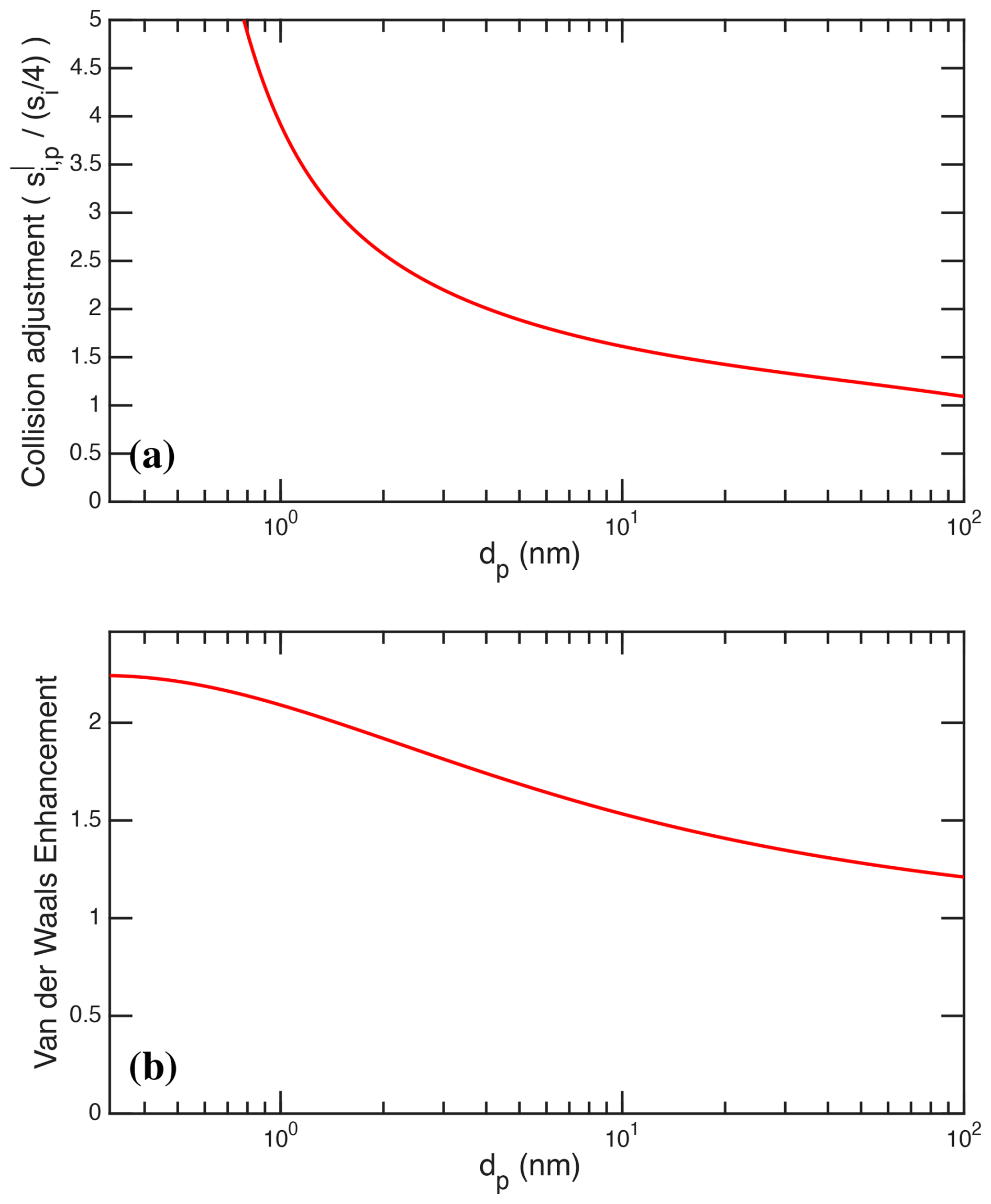
Figure 5 Enhancement over simple kinetic condensation vs. size for H₂SO₄. (a) All effects adjusting simple vapor condensation speed, ${\stackrel{\mathrm{‾}}{s}}_{{\mathrm{H}}_{\mathrm{2}}{\mathrm{SO}}_{\mathrm{4}}}/\mathrm{4}$. (b) Van der Waals enhancement alone for $A_{{\mathrm{H}}_{\mathrm{2}}{\mathrm{SO}}_{\mathrm{4}}}=\mathrm{6}\times {\mathrm{10}}^{-\mathrm{20}}$ J to give $E_{{\mathrm{H}}_{\mathrm{2}}{\mathrm{SO}}_{\mathrm{4}}}^{\mathit{\mu }}\simeq \mathrm{1.6}$ at d_p=10 nm.

5.2.3 Calibrating the condensation sink

Figure 6 shows the observed particle size distributions from combined DMA-train, nano-SMPS, and SMPS data as “bunches of bananas” of both the number distribution and the condensation sink distribution, as well as the resulting integrated number distribution and condensation sink for Run 1833. We apply median filters and interpolants to the scalar values in the lower panels to reduce the scatter. To match the CPC_2.5 total number, we scale data from the SMPS (for d_p≳7.2 nm) by ${\mathcal{F}}_{\mathrm{SMPS}}^{\mathrm{cal}}=\mathrm{1.33}$, consistent with a small undercounting for the SMPS (the peak hues in the distribution are modestly darker than in Fig. 2). With this, the integrated distributions match the CPC_2.5 regardless of whether most of the particles are principally small (d_p<10 nm) or large (d_p>10 nm). Only when the particles are very small is there some hint of an discrepancy between the CPC_2.5 and the integrated distribution (mostly the DMA train under these conditions). Here some consideration of the CPC_2.5 transmission curve might be warranted, but for the vast majority of the time, with larger particles, the agreement between the CPC_2.5 and the integrated size distribution (after correcting for the SMPS undercount) is well better than 10 %, giving high confidence in the size distribution over time and thus both the total number and the integrated surface area.

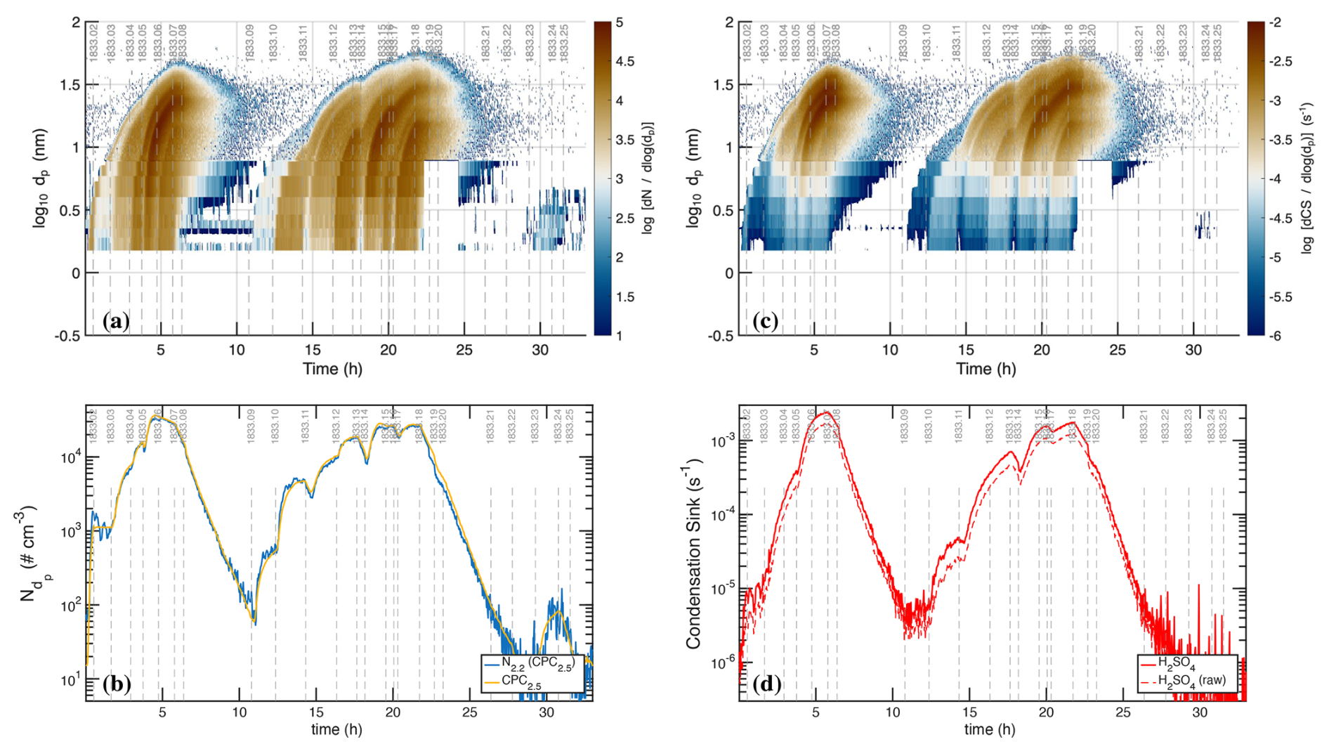
Figure 6 Particle measurements after scaling to match CPC_2.5 values. (a) Particle size distribution ($\mathrm{d}N/\mathrm{d}\log d_{\mathrm{p}}$) after calibration. (b) The total particle number for d_mob≥2.5 nm (d_p≥2.2 nm) measured with a TSI CPC_2.5 as well as the integrated number distribution after calibration. SMPS data for d_p≥7.1 nm are scaled by 1.33 to match the CPC_2.5 data; the constraints are especially tight for loss stages 07-08 and 18-20, where almost all of the particles were d_p>10 nm (though in portions of stages 18-20 the DMA-train data are missing). (c) condensation sink distribution ($\mathrm{dCS}/\mathrm{d}\log d_{\mathrm{p}}$) after calibration. (d) The integrated condensation sink after SMPS calibration. The solid red curve shows the condensation sink for H₂SO₄ including a Hamaker (Van der Waals) constant of $\mathrm{6}\times {\mathrm{10}}^{-\mathrm{20}}$ J whereas the dashed red curve omits this, revealing a roughly 30 % Van der Waals enhancement.

Various modes of nucleation and growth are clearly evident during both the UVH and UVX stages. Stage 02, which is neutral with low H₂SO₄, shows little nucleation, and stage 06, which is charged, shows less nucleation than the preceding neutral stage 05. Each of the visible nucleation bursts forms individual nucleation modes, whose growth rates must be proportional to the absolute amount of condensation, which in turn depends on the absolute H₂SO₄ concentration. During both events, these bunches of bananas reach a maximum size of d_p≃30 nm.

The Van der Waals term maximizes for objects of the same size (Chan and Mozurkewich, 2001), but the enhancement is substantial throughout the 5–15 nm size range most relevant here, increasing the collision rate by roughly 60 % at 10 nm. Overall the sharp deceleration in collision speed with size shown in Fig. 5a is essential to reproduce the sharp modal shape of the bunches of bananas we observe. Without this condensational narrowing the nucleation modes would remain much more spread out towards lower size. The condensation sink for H₂SO₄ obtained from these calibrated size distributions, including the Van der Waals effect, agrees very closely with the observed gas-phase H₂SO₄ signals. Complementary model runs, without the condensational narrowing induced by the Van der Walls term, fail to reproduce these well-defined modes.

Figure 6d shows the measured condensation sink vs. time for H₂SO₄ with (solid) and without (dashed) the Van der Waals correction. The corrected condensation sink, with integrated particle number matching the CPC_2.5 and treatment of the Van der Waals enhancement, provides our best a-priori estimate of the condensation contribution to the first-order H₂SO₄ loss term.

Figure 6 and especially Fig. 6b and d comprise a two-moment objective function to assess the agreement between different measurements and between measurements and simulations incorporating various calibration terms, ${\mathcal{F}}_i^{\mathrm{cal}}$. For an optimal calibration, we would quantify this performance (including some weighting of the variance between the different moments of the simulated and observed distributions) and obtain optimal ${\mathcal{F}}_i^{\mathrm{cal}}$ along with a full variance-covariance matrix. Here however we shall restrict ourselves to a “by eye” comparison of these four panels to assess different simulations.

6 H₂SO₄ Loss Calibration

With the first-order condensation sink calibrated we could assess the production and loss balance of H₂SO₄, assuming that $P_{{\mathrm{H}}_{\mathrm{2}}{\mathrm{SO}}_{\mathrm{4}}}\propto s_{\mathrm{lt}}$ for a given light source, lt. Here we show results from a full photochemical model, described in detail below, but at this step in the calibration sequence our focus is on accurate constraint of the first-order loss (largely wall loss and condensation), which provides a precise constraint of $P_{{\mathrm{H}}_{\mathrm{2}}{\mathrm{SO}}_{\mathrm{4}}}$ and thus $c_{{\mathrm{H}}_{\mathrm{2}}{\mathrm{SO}}_{\mathrm{4}}}$ (the shape, but not absolute amount). The actual scale of $c_{{\mathrm{H}}_{\mathrm{2}}{\mathrm{SO}}_{\mathrm{4}}}$ (i.e. ${\mathcal{F}}_{{\mathrm{H}}_{\mathrm{2}}{\mathrm{SO}}_{\mathrm{4}}}^{\mathrm{cal}}$) remains to be determined, presuming (as is the case) that the shape of the concentration vs. time remains largely unchanged with modest scaling of the absolute concentration.

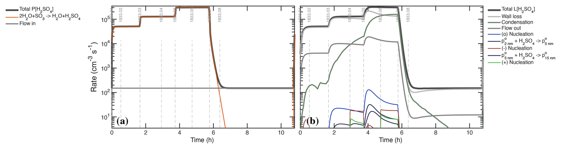
Figure 7 Production and loss rates of H₂SO₄ during the UVH stages. (a) Production rises in 3 steps with UVH intensity in stages 01–06 and then drops to near zero with the lights are turned off for stages 07 and 08. A small source of unknown origin is modeled as a constant flow more than 3 orders of magnitude lower than the maximum photochemical production. (b) Losses are dominated by wall deposition (light gray) and condensation (gray-green), with a small contribution from dilution (flow out, dark gray), giving the overall rate balance evident by comparing the two panels. Losses from nucleation itself are evident but extremely small.

Figure 7 shows the production and loss rate balance for H₂SO₄ during the UVH stages of run 1833, including 3 different light intensities over 6 stages followed by two dark stages. This is the first of many process rate analyses from our suite of models; we show production and loss side-by-side with identical y-axes so the degree of balance can be assessed directly. Here the production and loss rates balance following a short adjustment after each step in UVH intensity (the loss rates adjust with a timescale given by $\mathrm{1}/k_{{\mathrm{H}}_{\mathrm{2}}{\mathrm{SO}}_{\mathrm{4}}}^{\mathrm{I}}$). The production rates are almost entirely photochemical (appearing as hydrolysis, ${\mathrm{SO}}_{\mathrm{3}}+\mathrm{2}{\mathrm{H}}_{\mathrm{2}}\mathrm{O}⟶{\mathrm{H}}_{\mathrm{2}}{\mathrm{SO}}_{\mathrm{4}}+{\mathrm{H}}_{\mathrm{2}}\mathrm{O}$ in Fig. 7a). The loss rates are predominantly wall loss, with steadily rising condensation and a small (few percent) contribution from dilution. Condensation exceeds wall loss in stage 06. During the “wall loss” stage 07 the condensation and wall loss rates remain nearly equal, and so the separation between wall loss and condensation is achieved primarily during stages 01–04, when condensation is at most 10 % of the wall loss rate, making these level steps with a precise (nearly constant) H₂SO₄ signal important in the separation. The shape of these production and especially loss curves constrains the absolute magnitude of the major loss processes.

There is a small unknown source of H₂SO₄, modeled here as a constant input flow. It is orders of magnitude weaker than photochemistry when the lights are on and so has no practical effect on the calibration. It could be an instrument background but it is shared by two instruments as seen in Fig. 2b, and because of this and its shape we conclude that it is real, of unknown origin, but of no further consequence because it is orders of magnitude smaller than the H₂SO₄ production during active photochemistry.

During the most intense nucleation events, nucleation remains less than 1 ‰ of the overall H₂SO₄ loss. The “nanoparticle” and “cluster” growth terms are part of overall condensation as it is treated in a modal scheme within the photochemical model; this would be double counting the condensation sink but they represent single collisions of H₂SO₄ with particles comprising those modes, and growth from one mode to the next requires hundreds to thousands of such collisions. These growth terms are many orders of magnitude smaller than the total condensation sink and so we can run the photochemical model with an externally constrained condensation sink – the measured values shown Fig. 8b – without introducing double counting error.

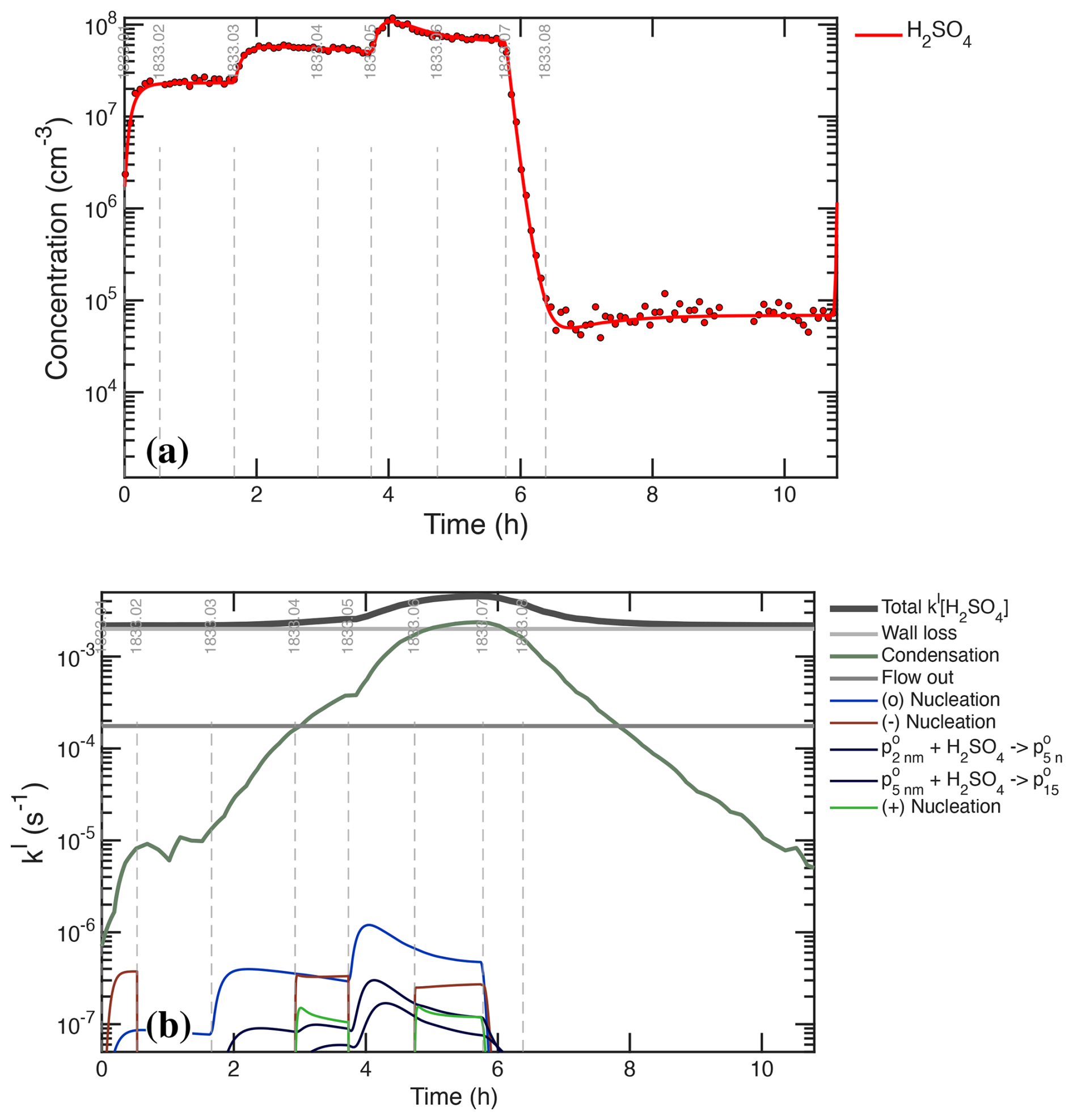
Figure 8 (a) H₂SO₄ concentration measurements (points) and model (curve) during the UVH stages. (b) H₂SO₄ first-order loss frequency (inverse lifetime). Wall loss defines the minimum loss frequency, with condensation contributing equally during the middle of the sequence. The H₂SO₄ steady state concentration falls during stages 05 and 06, with the model and measurements agreeing at all times.

Figure 8 compares the modeled and measured H₂SO₄ as well as the individual terms comprising the H₂SO₄ first-order loss. The condensation frequency shown in Fig. 8b corresponds to the condensation loss rate shown in Fig. 7b. Accurate separation of wall and condensation loss requires that the condensation loss grows to at least equal the wall loss, such as during stages 05–07. This is important for two reasons. First, stage 07 is a so-called “wall loss” stage with no H₂SO₄ production, but the condensation sink remains competitive, meaning that k^wall+k^cond are constrained jointly during this stage. The wall loss itself is more tightly constrained by the steady-state H₂SO₄ levels during e.g. stages 02–03, when the condensation sink is negligible. Second, the progressive drop in the steady-state H₂SO₄ during stages 05–06 requires this competition between wall and condensation losses and is not consistent with a lower condensation sink (without the Van der Waals enhancement). The particle number (or individual particle surface area) could be increased by 30 % to achieve the same effect, but the condensation sink itself is tightly constrained. Because we regard the CPC_2.5 as accurate and because the Van der Waals effect produces modes with the right shape (discussed below), we conclude that the current constraints are correct (to within roughly 10 %), meaning ${\mathcal{F}}_{\mathrm{cond}}^{\mathrm{cal}}\simeq \mathrm{1.0}\pm \mathrm{0.1}$. Overall the modeled H₂SO₄ matches measurements for all light intensities after the wall loss is constrained (to its nominal value), with ${\mathit{\tau }}_{{\mathrm{H}}_{\mathrm{2}}{\mathrm{SO}}_{\mathrm{4}}}^{\mathrm{wall}}=\mathrm{500}\mathrm{s}$ and ${\mathcal{F}}_{\mathrm{wall}}^{\mathrm{cal}}\simeq \mathrm{1.0}\pm \mathrm{0.1}$.

Figure 8a shows that the H₂SO₄ signals precisely match the expected (modeled) signals, and the lower panel shows the individual contributions to the H₂SO₄ loss frequency. The constant wall and dilution frequencies stand in contrast to the evolving condensation loss term. The overall rate balance in Fig. 7 and the precise fit of H₂SO₄ in Fig. 8a combine to give a strong and accurate constraint on the two timescales (wall and condensation loss) in Fig. 8b. Even the small depression in the H₂SO₄ signal at the start of cleaning stage 08 is consistent with the model – the H₂SO₄ steady state increases as the constant (unknown) source is balanced by an increasing lifetime as the condensation sink diminishes, which shows that the small unknown H₂SO₄ source is a real signal. The condensation frequency shown here is derived from the measured particle size distribution; however, the overall H₂SO₄ first-order loss, and thus the condensation frequency during the middle period of the UVH stages where the total loss rises well above the wall loss timescale, is accurately constrained regardless of any particle measurements. The constrained condensation sink thus becomes a powerful constraint for the calibration of those particle measurements, and the constrained condensation sink then provides a separate constraint for the absolute H₂SO₄ because the growth via condensation is required to generate the condensation sink.

7 Nucleation and Growth

The H₂SO₄ loss is accurately constrained, in part by the equally well constrained total particle number and size distribution forming the condensation sink. The next step is to determine the absolute H₂SO₄ calibration factor required to nucleate and grow those particles to sufficient number and size to form that sink. The condensation sink is determined by the number of particles with surface area – the total suspended surface area – and so it depends on both the nucleation and growth of particles (as well as their sinks). Nucleation and growth are connected of course – without particle formation there is nothing to grow.

To constrain nucleation and growth, we employ two tools. One is a sectional microphysical model described in detail elsewhere (Donahue et al., 2019). The other is a comprehensive gas-phase photochemical model described below that contains a simple modal scheme to represent particles, including ions and charge. The sectional microphysical model does not (yet) represent the charge state of particles. The major connection between gas-phase processes and aerosol microphysics in this experiment is the H₂SO₄ vapor concentration and the aerosol condensation sink of that H₂SO₄, and so the different modules can be driven either by modeled or observational data. For example, the microphysical model can be driven by measured H₂SO₄ (with a potential calibration factor), and the gas-phase photochemical model can incorporate the observed condensation sink (as shown in Fig. 8b). The two models provide complementary constraints and together enable a comprehensive analysis of the processes connecting the fully coupled system. We do not run a fully coupled model as there is no real point. The purpose of the gas-phase model is to reproduce the observed H₂SO₄ (and ultimately thus constrain the OH and UV light intensities); the purpose of the microphysical model is to reproduce the observed particle number and size distribution, once the observed and modeled H₂SO₄ agree.

Particle sections in the microphysical model have spherical equivalent diameter, d_p, and track number concentration (n_p) and composition via density (ρ_p) and constituent specific volume (v_i,p) and thus constituent mass concentration ($m_{i,p}={\mathit{\rho }}_{\mathrm{p}}{v}_{i,p}$). Density can be specified for each species if the particles have more than one phase, but in this case we assume a single condensed phase in each bin. The model treats condensational growth with a moving sectional algorithm and user-selectable size limits, $d_{\min }\le d_{\mathrm{p}}\le d_{\max }$ and resolution, δlog ₁₀d_p. At the end of each growth step the algorithm redistributes particles to the specified sizes, conserving number and mass by distributing particles between the fixed bins below and above each new particle size. The model treats coagulation, again conserving number and mass when the produced particles inevitably fall between the fixed size bins. Finally, the model treats size dependent wall loss and size independent ventilation loss.

Because the current microphysical model does not treat particle charge, it cannot treat coagulation or wall loss enhancements due to charge. The most obvious manifestation of enhanced loss is the sudden removal of charged particles when the clearing field is turned on after a stage with charge (e.g. the start of stage 02 and especially stage 05). As already discussed, most of the particles are neutral even during charged stages with substantial ion induced nucleation because the growing particles are neutralized via diffusion (dis)charging. However, at the start of these neutral stages some 10 %–20 % of the particles are charged (as seen in Fig. 3). We address this empirically by removing a fraction of the particles, independent of size, at the start of these stages. This is crude, but because the fraction removed is small, errors caused by this crude treatment are negligible.

7.1 Nucleation

The models treat nucleation with either fixed nucleation rates (J) or externally specified vapor concentrations (H₂SO₄, NH₃, H₂O and ions). Those may be from observations or, in the case of the microphysical model, from the photochemical model. It is not the purpose of this study to constrain nucleation rates per se, but rather to constrain all other parameters leading up to an accurate determination of the nucleation rates. Here we shall simply adjust a nucleation coefficient in order to reproduce the observed particle number (increase) during each stage. We represent nucleation as formation of either neutral or singly charged clusters $c^{\circ ,-,+}$ via interactions of H₂SO₄, NH₃, and ions (n^±). The nucleation rate is nearly third-order in H₂SO₄ and nearly first-order in NH₃ (Dunne et al., 2016; Gordon et al., 2017); here we treat nucleation as exactly third and first order but then adjust the nucleation coefficients for each stage, $k_{\mathrm{n}},k_{\pm }$.

$$\begin{array}{c}{\displaystyle }{J}_{\mathrm{1.7}}^{\circ }=k_{\mathrm{n}}{c}_{{\mathrm{H}}_{\mathrm{2}}{\mathrm{SO}}_{\mathrm{4}}}^{\mathrm{3}}{c}_{{\mathrm{NH}}_{\mathrm{3}}}\\ {\displaystyle }{J}_{\mathrm{1.7}}^{\mathrm{ion}}=k_{\pm }{c}_{{\mathrm{H}}_{\mathrm{2}}{\mathrm{SO}}_{\mathrm{4}}}^{\mathrm{3}}{c}_{{\mathrm{NH}}_{\mathrm{3}}}{n}^{\pm }\end{array}$$

We assume that the ion-induced channel is linear in the concentration of ions (n^±) and predominantly negative, but we treat a fraction of positive ion nucleation based on the observed depletion of the positive primary ions. The ions themselves are produced via an ion-pair production rate, J^ip=7 cm⁻³ s⁻¹, which as we shall see later is sufficient to sustain a steady state $c_{n^{-}}\simeq c_{n^{+}}=\mathrm{1500}$ cm⁻³, as seen in Fig. 3c, f. In the microphysical model, nucleated particles are introduced at an initial particle size, d_p=0.8 nm.

The photochemical model treats ions and thus calculates nucleation directly. The microphysical model does not explicitly treat ions, and so we have two choices. The first choice is to fix the ion concentrations at the observed $n^{-}=\mathrm{1500}$ cm⁻³ but to ensure that the derived ion induced nucleation rate does not exceed the ion pair limit by imposing a saturation constraint:

$$\begin{array}{}\text{(4)}& J^{\mathrm{iin}}={\displaystyle \frac{\mathrm{1}}{\frac{\mathrm{1}}{J^{\mathrm{ion}}}+\frac{\mathrm{1}}{J^{\mathrm{ip}}}}}\end{array}$$

This has the same effect as the expected depletion of ion concentrations as nucleation becomes a major ion sink, but it omits other possible interactions. The second choice is to use an interpolant of constrained ion concentrations (either from measurements or the photochemical model), with a limit to ensure Jⁱⁱⁿ≤J^ip. As we shall see, nucleation rates from the two models agree well when we apply the saturation constraint, and so that is our default choice.

7.2 Condensational growth

The condensation sink contributes to first-order loss of H₂SO₄, but in turn it drives particle growth. While the growth rate is governed by H₂SO₄ condensation, co-condensation of other vapors (NH₃ and perhaps H₂O) must also be addressed to constrain the growth of the size distribution. We also assume that the measured size distribution shown in Fig. 6 accurately reflects their true size in CLOUD.

The condensation sink is generated both by nucleation (to produce particle number) and growth (to produce particle surface area), which we can constrain with the dual constraints of total particle number (the CPC_2.5) and condensation sink. For this step we shall restrict the figures to these UVH stages (01–08), as this is sufficient for the constraint, takes less time to simulate, and the figures are easier to read with this narrower time range (we conducted the same analysis for the UVX stages, some of which is presented in the Supplement). Stages 01, 04, and 06 are charged while 02, 03 and 05 are neutral. Stage 08 is a cleaning stage with the beam on 50 % but the clearing field alternating between off and on in order to build up charge on larger particles and then sweep them from the chamber.

7.2.1 Condensation of volatile species

The condensation flux per unit surface area from the vapor (v) to a suspended phase (s), of a species (i) to a particle population (p), is ${\mathit{\varphi }}_{i,p}^{\mathrm{v},\mathrm{s}}$. This depends on an excess concentration, $c_{i,p}^{\mathrm{xs}}$. For effectively non-volatile species, such as sulfuric acid in this case, this is just the vapor concentration: $c_{i,p}^{\mathrm{xs}}=c_i^{\mathrm{v}}$. That is further ensured when reactive uptake with unit uptake coefficient (${\mathit{\gamma }}_i^{\mathrm{rxn}}=\mathrm{1}$) converts the condensing vapor to a non-volatile salt (in this case ammonium salts, ${\mathrm{H}}_{\mathrm{2}}{\mathrm{SO}}_{\mathrm{4}}+n{\mathrm{NH}}_{\mathrm{3}}⟶\left({\mathrm{H}}_{\mathrm{2}-n}{\mathrm{SO}}_{\mathrm{4}}\right)-({\mathrm{NH}}_{\mathrm{4}}{)}_n$).

When species are volatile, evaporation (net condensation) depends on the volatility of the vapor species (saturation concentration $c_i^{\circ }$) as well as its activity in the suspended particle ($a_{i,p}^{\mathrm{s}}$).

$$\begin{array}{c}{\displaystyle }{c}_{i,p}^{\mathrm{xs}}=c_i^{\mathrm{v}}\left(\mathrm{1}-{\displaystyle \frac{c_i^{\circ }}{c_i^{\mathrm{v}}}}{a}_{i,p}^{\mathrm{s}}\right)\\ {\displaystyle }{a}_{i,p}^{\mathrm{s}}=K_{i,p}{\mathit{\gamma }}_{i,p}{x}_{i,p}\end{array}$$

Here that applies to both ammonia (via reactive uptake) and water. The Kelvin term (K_i,p) accounts for increased vapor pressure over highly curved small particles. This can be expressed in terms of a “decadal Kelvin diameter”, d_K10, which is the diameter at which the vapor pressure is a factor of 10 higher than over a flat surface.

$$\begin{array}{c}{\displaystyle }{\log }_{\mathrm{10}}{K}_{i,p}=\left({\displaystyle \frac{d_{\mathrm{K}\mathrm{10}}}{d_{\mathrm{p}}}}\right)+O{\left({\displaystyle \frac{d_{\mathrm{K}\mathrm{10}}}{d_{\mathrm{p}}}}\right)}^{\mathrm{2}}+\mathrm{\dots }\\ {\displaystyle }{d}_{\mathrm{K}\mathrm{10}}=\mathrm{0.434}{d}_K;d_K=\left({\displaystyle \frac{\mathrm{4}{\mathit{\sigma }}_p{m}_i}{k_{\mathrm{B}}T{\mathit{\rho }}_{\mathrm{p}}}}\right)=\left({\displaystyle \frac{\mathrm{4}{\mathit{\sigma }}_p{V}_i}{RT}}\right)\end{array}$$

For water, with M_i≃18 amu, σ_p≃80 mN m⁻¹ and ρ_p≃1000 kg m⁻³, d_K10=1 nm.

7.2.2 Growth rate

The model is driven by the condensation flux, but it is useful to consider the growth rate. This speed ($s_{i,p}^{\mathrm{gr}}$ assuming a particle with spherical equivalent d_p) due to the flux, ${\mathit{\varphi }}_{i,p}^{\mathrm{v},\mathrm{s}}$, of a constituent with molar mass M_i into a phase with density ρ_p, and thus with molar volume $v_i=M_i/{\mathit{\rho }}_{\mathrm{p}}$, is:

$$s_{i,p}^{\mathrm{gr}}=\mathrm{2}{\displaystyle \frac{M_i}{{\mathit{\rho }}_{\mathrm{p}}}}{\mathit{\varphi }}_{i,p}^{\mathrm{v},\mathrm{s}}=\mathrm{2}{v}_i{\mathit{\varphi }}_{i,p}^{\mathrm{v},\mathrm{s}};s_p^{\mathrm{gr}}=\sum _i{s}_{i,p}^{\mathrm{gr}}$$

The factor of 2 is because growth extends the diameter by extending the radius symmetrically.

7.2.3 Co-condensation of abundant vapors

For ternary H₂SO₄, NH₃ and H₂O nucleation and growth, condensational growth is rate limited by H₂SO₄ condensation but is accompanied by NH₃ and H₂O. This can have two subtly different manifestations: vapors can co-condense with a fixed stoichiometric ratio to H₂SO₄ via reactive uptake (i.e. 2 : 1 for ${\mathrm{H}}_{\mathrm{2}}{\mathrm{SO}}_{\mathrm{4}}+\mathrm{2}{\mathrm{NH}}_{\mathrm{3}}⟶({\mathrm{NH}}_{\mathrm{4}}{)}_{\mathrm{2}}\cdot {\mathrm{SO}}_{\mathrm{4}}$); or vapors can continuously approach equilibrium with the condensed-phase solution to maintain equal activities in both vapor and condensed phases (i.e. $a_{{\mathrm{H}}_{\mathrm{2}}\mathrm{O}}⟶\mathrm{RH}/\mathrm{100}$). In either event, the other vapors will contribute to the particle volume in proportion to their molar volume, so scaled by their molar mass, $M_i/M_{{\mathrm{H}}_{\mathrm{2}}{\mathrm{SO}}_{\mathrm{4}}}$.

Here we assume the ammonia co-condenses with a 2:1 stoichiometry but is in sufficient excess to maintain its equilibrium composition (activity) in the growing particles, regardless of whether they are wet or dry and regardless of size: Specifically, if NH₃ condenses with a stoichiometry of $s_{{\mathrm{NH}}_{\mathrm{3}}}$ with respect to H₂SO₄:

$$\begin{array}{rl}{s}_p^{\mathrm{gr}}& =\mathrm{2}\left({\displaystyle \frac{M_{{\mathrm{H}}_{\mathrm{2}}{\mathrm{SO}}_{\mathrm{4}}}}{{\mathit{\rho }}_{\mathrm{p}}}}{\mathit{\varphi }}_{{\mathrm{H}}_{\mathrm{2}}{\mathrm{SO}}_{\mathrm{4}},p}^{\mathrm{v},\mathrm{s}}+{\displaystyle \frac{M_{{\mathrm{NH}}_{\mathrm{3}}}}{{\mathit{\rho }}_{\mathrm{p}}}}{\mathit{\varphi }}_{{\mathrm{NH}}_{\mathrm{3}},p}^{\mathrm{v},\mathrm{s}}\right)\\ & =\mathrm{2}\left({\displaystyle \frac{M_{{\mathrm{H}}_{\mathrm{2}}{\mathrm{SO}}_{\mathrm{4}}}+s_{{\mathrm{NH}}_{\mathrm{3}}}{M}_{{\mathrm{NH}}_{\mathrm{3}}}}{{\mathit{\rho }}_{\mathrm{p}}}}\right){\mathit{\varphi }}_{{\mathrm{H}}_{\mathrm{2}}{\mathrm{SO}}_{\mathrm{4}},p}^{\mathrm{v},\mathrm{s}}\end{array}$$

However, the very smallest particles, visible in an Atmospheric Pressure Interface Time of Flight Mass Spectrometer (APITOF), have been shown to grow with a 1 : 1 stoichiometry (i.e. as ammonium bisulfate) (Kirkby et al., 2011); this is presumably due to a Kelvin effect for extremely small particles (Ahlm et al., 2016). It is not yet known over what size range $s_{{\mathrm{NH}}_{\mathrm{3}}}$ changes from 1 to 2, but here we assume it is below the size range where our analysis is most sensitive to our constraints on growth rate. None the less the smallest particles are likely to be ammonium bisulfate, which may well matter to the overall behavior at any given relative humidity.

Condensation of H₂O represents a binary uncertainty in these calculations. At thermodynamic equilibrium and 58 % RH, the particles would grow as dry (NH₄)₂−SO₄, as this is well below the 80 % deliquescence relative humidity (DRH), which persists down to d_p≃6 nm (Lei et al., 2020). If the particles are dry, they contain essentially no water and have a hygroscopic growth factor very near 1.0 and $s_{{\mathrm{H}}_{\mathrm{2}}\mathrm{O}}\simeq \mathrm{0}$ (Bezantakos et al., 2016). This would also imply that any sample drying during sampling (i.e. due to dry sheath flow) would have minimal effect on the already dry particles.

However, the particles initially grow as ammonium bisulfate, and particles with stoichiometry between 1 : 1 and 1.5 : 1 have a DRH as low as 37 % down to d_p=15 nm, (Mifflin et al., 2009). The nucleated particles may well grow as aqueous (deliquesced) particles and so remain wet during growth even once the stoichiometry increases to 2 : 1, because 58 % RH is well above the efflorescence relative humidity of ammonium sulfate. Further, the growth rate of particles observed under similar conditions in CLOUD is independent of NH₃ for $\mathrm{1}\lesssim {\mathit{\chi }}_{{\mathrm{NH}}_{\mathrm{3}}}<\mathrm{1000}$ ppt (Stolzenburg et al., 2020), thus encompassing pure sulfuric acid droplets. Because H₂O almost certainly condenses to H₂SO₄ droplets at very low NH₃, we conclude that the particles in Run 1833 were also wet. If they did grow along the meta-stable deliquescence branch as a deliquesced aqueous solution, their diameter growth factor was roughly 1.2 (depending on size) (Lei et al., 2020; Vlasenko et al., 2017), and they sustained a water activity of $a_{{\mathrm{H}}_{\mathrm{2}}\mathrm{O}}^{\mathrm{s}}=\mathrm{0.58}$. This will also have implications for the accuracy of the measured particle size distribution, as the SMPS measurement may involve some drying in the DMA column (Stolzenburg et al., 2020). However, the condensation sink remains precisely constrained by the directly observed contribution to first-order H₂SO₄ vapor loss.

Our treatment of water condensation in the growth will be to sustain the water activity via simplified thermodynamics, but consideration of hygroscopic growth is useful to check this treatment. The growth factor can be split into two contributing elements. One is the density difference between the aqueous and dry particles; the other is the contribution of condensing water to the overall molar volume. Both affect volume and so the volume growth factor $f_{\mathrm{gr}}^{\mathrm{3}}$.

$$\begin{array}{rl}{f}_{\mathrm{gr}}^{\mathrm{3}}=& \left({\displaystyle \frac{{\mathit{\rho }}_{\mathrm{dry}}}{{\mathit{\rho }}_{\mathrm{wet}}}}\right)\times \\ & \left({\displaystyle \frac{M_{{\mathrm{H}}_{\mathrm{2}}{\mathrm{SO}}_{\mathrm{4}}}+s_{{\mathrm{NH}}_{\mathrm{3}}}{M}_{{\mathrm{NH}}_{\mathrm{3}}}+s_{{\mathrm{H}}_{\mathrm{2}}\mathrm{O}}{M}_{{\mathrm{H}}_{\mathrm{2}}\mathrm{O}}+{\sum }_i{s}_i{M}_i}{M_{{\mathrm{H}}_{\mathrm{2}}{\mathrm{SO}}_{\mathrm{4}}}+s_{{\mathrm{NH}}_{\mathrm{3}}}{M}_{{\mathrm{NH}}_{\mathrm{3}}}}}\right)\\ =& \left({\displaystyle \frac{{\mathit{\rho }}_{\mathrm{dry}}}{{\mathit{\rho }}_{\mathrm{wet}}}}\right)\left(\mathrm{1}+{\displaystyle \frac{s_{{\mathrm{H}}_{\mathrm{2}}\mathrm{O}{\sum }_i{s}_i{M}_i}{M}_{{\mathrm{H}}_{\mathrm{2}}\mathrm{O}}}{M_{{\mathrm{H}}_{\mathrm{2}}{\mathrm{SO}}_{\mathrm{4}}}+s_{{\mathrm{NH}}_{\mathrm{3}}}{M}_{{\mathrm{NH}}_{\mathrm{3}}}}}\right)\end{array}$$

The term ∑_is_i M_i accounts for other constituents, such as H⁺ and ${\mathrm{HSO}}_{\mathrm{4}}^{-}$, which we lump into H₂O and H₂SO₄ and otherwise neglect in this simple treatment. This is reasonable for neutral (NH₄)₂−SO₄. Thus, for a known growth factor, the molar ratio of H₂O to H₂SO₄ is

$$s_{{\mathrm{H}}_{\mathrm{2}}\mathrm{O}}=\left(f_{\mathrm{gr}}^{\mathrm{3}}\left({\displaystyle \frac{{\mathit{\rho }}_{\mathrm{wet}}}{{\mathit{\rho }}_{\mathrm{dry}}}}\right)-\mathrm{1}\right)\left({\displaystyle \frac{M_{{\mathrm{H}}_{\mathrm{2}}{\mathrm{SO}}_{\mathrm{4}}}+s_{{\mathrm{NH}}_{\mathrm{3}}}{M}_{{\mathrm{NH}}_{\mathrm{3}}}}{M_{{\mathrm{H}}_{\mathrm{2}}\mathrm{O}}}}\right)$$

For example, at 58 % RH and $s_{{\mathrm{NH}}_{\mathrm{3}}}=\mathrm{2}$, the growth factor at d_p=100 nm is f^gr=1.27 (Lei et al., 2020). With ρ_dry=1770 kg m⁻³ and ρ_wet=1350 kg m⁻³, this gives $s_{{\mathrm{H}}_{\mathrm{2}}\mathrm{O}}=\mathrm{4.12}$, close to the EAIM value of $s_{{\mathrm{H}}_{\mathrm{2}}\mathrm{O}}=\mathrm{4.36}$ (Friese and Ebel, 2010). Tandem-DMA measurements of (NH₄)₂⋅SO₄ hygroscopic growth show growth factors consistent with established thermodynamics and a size dependence affected by a Kelvin term (Lei et al., 2020). For this reason we shall assume that the particles rapidly equilibrate with water vapor to maintain a particle activity equal to the ambient RH (58 % in this case).

To find the equilibrium water activity, we equilibrate each particle section after it grows due to condensation of H₂SO₄ and so find the molar ratio of H₂O to to H₂SO₄, $s_{{\mathrm{H}}_{\mathrm{2}}\mathrm{O}}$. The mole fraction of water is

$$\begin{array}{c}{\displaystyle }{x}_{{\mathrm{H}}_{\mathrm{2}}\mathrm{O}}={\displaystyle \frac{s_{{\mathrm{H}}_{\mathrm{2}}\mathrm{O}}}{\mathrm{1}+s_{{\mathrm{NH}}_{\mathrm{3}}}+s_{{\mathrm{H}}_{\mathrm{2}}\mathrm{O}}}}\\ {\displaystyle \frac{\mathrm{1}}{x_{{\mathrm{H}}_{\mathrm{2}}\mathrm{O}}}}=\left(\mathrm{1}+{\displaystyle \frac{\mathrm{1}+s_{{\mathrm{NH}}_{\mathrm{3}}}}{s_{{\mathrm{H}}_{\mathrm{2}}\mathrm{O}}}}\right)\end{array}$$

so the molar ratio of water to H₂SO₄ is

$$\begin{array}{rl}{s}_{{\mathrm{H}}_{\mathrm{2}}\mathrm{O}}& ={\displaystyle \frac{\mathrm{1}+s_{{\mathrm{NH}}_{\mathrm{3}}}}{\frac{\mathrm{1}}{x_{{\mathrm{H}}_{\mathrm{2}}\mathrm{O}}}-\mathrm{1}}}\\ & =x_{{\mathrm{H}}_{\mathrm{2}}\mathrm{O}}{\displaystyle \frac{\mathrm{1}+s_{{\mathrm{NH}}_{\mathrm{3}}}}{\mathrm{1}-x_{{\mathrm{H}}_{\mathrm{2}}\mathrm{O}}}}\end{array}$$

This is then governed by the water activity, including the Kelvin term and any activity coefficient, ${\mathit{\gamma }}_{{\mathrm{H}}_{\mathrm{2}}\mathrm{O},p}$.

$$x_{{\mathrm{H}}_{\mathrm{2}}\mathrm{O},p}={\displaystyle \frac{a_{{\mathrm{H}}_{\mathrm{2}}\mathrm{O}}}{{\mathit{\gamma }}_{{\mathrm{H}}_{\mathrm{2}}\mathrm{O},p}{K}_{{\mathrm{H}}_{\mathrm{2}}\mathrm{O},p}}}$$

A full and accurate model requires (iterative) treatment of the thermodynamics (for example in the model MABNAG (Yli-Juuti et al., 2013; Ahlm et al., 2016)), but we find that simplified treatment with just H₂SO₄, NH₃ and H₂O, assuming ${\mathit{\gamma }}_{{\mathrm{H}}_{\mathrm{2}}\mathrm{O},p}\simeq \mathrm{1}$ reasonably reproduces the observed size-dependent growth factors for ammonium sulfate (Lei et al., 2020). For our default analysis, we shall thus assume that NH₃ condenses with a constant ratio to H₂SO₄ of 2 : 1 and water vapor equilibrates with particles to maintain $a_{{\mathrm{H}}_{\mathrm{2}}\mathrm{O}}=\mathrm{RH}$, with the wet particle density fixed at ρ_wet=1350 kg m⁻³ and a surface tension σ_p=79 mN m⁻¹ (Hyvärinen et al., 2005).

7.3 Coupled nucleation and growth simulations

We simulate the evolving particle size distribution with nucleation and condensation driven by H₂SO₄, finding the nucleation coefficients for each stage and scaling the sulfuric acid concentration by ${\mathcal{F}}_{{\mathrm{H}}_{\mathrm{2}}{\mathrm{SO}}_{\mathrm{4}}}^{\mathrm{cal}}$. The coefficients vary over the broad steps in H₂SO₄ because nucleation is not exactly third order in H₂SO₄ (Gordon et al., 2017). Nucleation governs total particle number (balanced by deposition and some coagulation), while growth rate-limited by H₂SO₄ condensation determines the condensation sink associated with that total number. Because the growth and nucleation are coupled in this way, we determine a nucleation coefficient for each stage to optimally match the particle number production during that stage (including wall and condensation loss of course) and then to constrain $F_{{\mathrm{H}}_{\mathrm{2}}{\mathrm{SO}}_{\mathrm{4}}}^{\mathrm{cal}}$ based on growth of the observed particle number to reproduce the observed condensation sink.

7.3.1 Calibrated model with wet (NH₄)₂-SO₄-(H₂O)_n growth

If we assume that H₂SO₄ condensation governs particle growth as wet $({\mathrm{NH}}_{\mathrm{4}}{)}_{\mathrm{2}}\cdot {\mathrm{SO}}_{\mathrm{4}}\cdot ({\mathrm{H}}_{\mathrm{2}}\mathrm{O}{)}_n$, the nominal (independently calibrated) H₂SO₄ drives particle growth that nearly matches the observations. Specifically, our best estimate is ${\mathcal{F}}_{{\mathrm{H}}_{\mathrm{2}}{\mathrm{SO}}_{\mathrm{4}}}^{\mathrm{cal}}\simeq \mathrm{1.15}\pm \mathrm{0.1}$, summarized in Fig. 9. Figure 9a shows the observed particle size distribution and Fig. 9b shows the integrated particle number for d_p≥2.2 nm along with the observed CPC_2.5 number. For this simulation we worked through the stages, adjusting the nominal nucleation coefficients (third order in $c_{{\mathrm{H}}_{\mathrm{2}}{\mathrm{SO}}_{\mathrm{4}}}$) to match the CPC_2.5 observations (Fig. 9b) and then adjusting ${\mathcal{F}}_{{\mathrm{H}}_{\mathrm{2}}{\mathrm{SO}}_{\mathrm{4}}}^{\mathrm{cal}}$ to match the observed condensation sink (Fig. 9d). Figure 9b shows the corresponding condensation sink distribution and Fig. 9d shows the modeled and observed condensation sink, with the calibrated Hamaker Constant $A_{{\mathrm{H}}_{\mathrm{2}}{\mathrm{SO}}_{\mathrm{4}}}=\mathrm{6}\times {\mathrm{10}}^{-\mathrm{20}}$ J, growth as wet $({\mathrm{NH}}_{\mathrm{4}}{)}_{\mathrm{2}}\cdot {\mathrm{SO}}_{\mathrm{4}}\cdot ({\mathrm{H}}_{\mathrm{2}}\mathrm{O}{)}_{\mathrm{2}}$ rate-limited by H₂SO₄ condensation, and nucleation described below. The overall agreement for particle number, growth rate (the size distribution), and condensation sink (the combination of number and size) remains within 10 % throughout, with the exception of losses during the cleaning stage (08), which this neutral microphysical model cannot reproduce. The very initial particle burst during stage 01 is also delayed, possibly because we treat the CPC_2.5 cutoff as a step function but the instrument has some sensitivity to smaller particles.

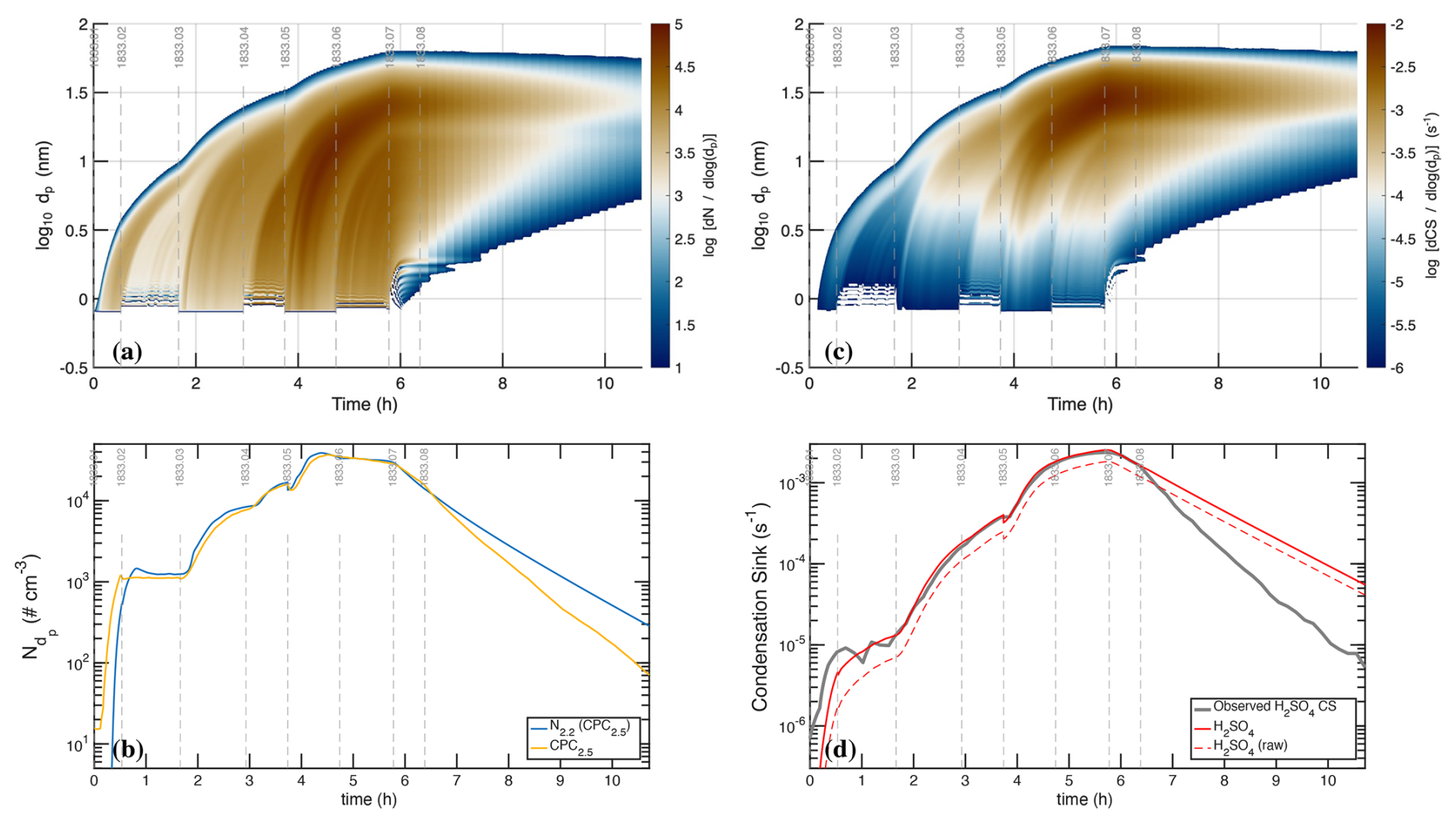
Figure 9 Optimal modeled particle size and corresponding condensation sink distributions with wet $({\mathrm{NH}}_{\mathrm{4}}{)}_{\mathrm{2}}-{\mathrm{SO}}_{\mathrm{4}}-({\mathrm{H}}_{\mathrm{2}}\mathrm{O}{)}_n$ growth, and their agreement with measurements. (a) Simulated particle size distribution ($\mathrm{d}N/\mathrm{d}\log d_{\mathrm{p}}$) for optimal parameters, with empirical nucleation coefficients and an H₂SO₄ calibration factor of 1.2. (b) Simulated (blue) and observed (gold) total particle number measurable by a CPC_2.5. The simulation for the most part agrees within 10 % of the observations, although it falls short during the low H₂SO₄ neutral stage 02. The simulation also does not include enhanced losses of charged particles and so misses the dip at the start of stage 05 as well as the accelerated loss during the cleaning stage 08. (c) Simulated condensation-sink distribution ($\mathrm{dCS}/\mathrm{d}\log d_{\mathrm{p}}$). (d) Simulated (red) and observed (gray) condensation sink. Simulated values are shown both with (solid) and without (dashed) a Van der Waals correction; the observed values include the correction; the condensation sink is reproduced with good fidelity aside from the enhanced loss during the cleaning stage, which was not simulated. Other than the low-intensity stages (01 and 02), charged and neutral nucleation are competitive because charged nucleation is limited by ion-pair production. That saturation value serves as an additional constraint on the nucleation parameters.

In Fig. 10a we show the observed size distribution for the UVX stages and in Fig. 10b we reproduce the modeled size distribution, again with ${\mathcal{F}}_{{\mathrm{H}}_{\mathrm{2}}{\mathrm{SO}}_{\mathrm{4}}}^{\mathrm{cal}}=\mathrm{1.15}$. This confirms the excellent model-measurement agreement for a different light source but shows minor differences. The empirical nucleation coefficients are for the most part similar to those for the UVH stages, and in all but one case (the medium intensity neutral stage 11), we found an optimal match with observed particle number with a small increase compared to the UVH stages. This is not surprising. The UVX light source is less uniform than the UVH source (Kupc et al., 2011), meaning $P_{{\mathrm{H}}_{\mathrm{2}}{\mathrm{SO}}_{\mathrm{4}}}$ will also be less homogeneous. This in turn will contribute to (small) inhomogeneities in $c_{{\mathrm{H}}_{\mathrm{2}}{\mathrm{SO}}_{\mathrm{4}}}$. Particle growth is slow and so uniform throughout the chamber. Because the H₂SO₄ calibration factors are identical for each case, we conclude that the measurements accurately reflect the average concentration. However, nucleation is (roughly) third order in H₂SO₄ and thus much more sensitive to spatial inhomogeneity of H₂SO₄ within the CLOUD chamber; this will tend to enhance the overall average nucleation rate as well.

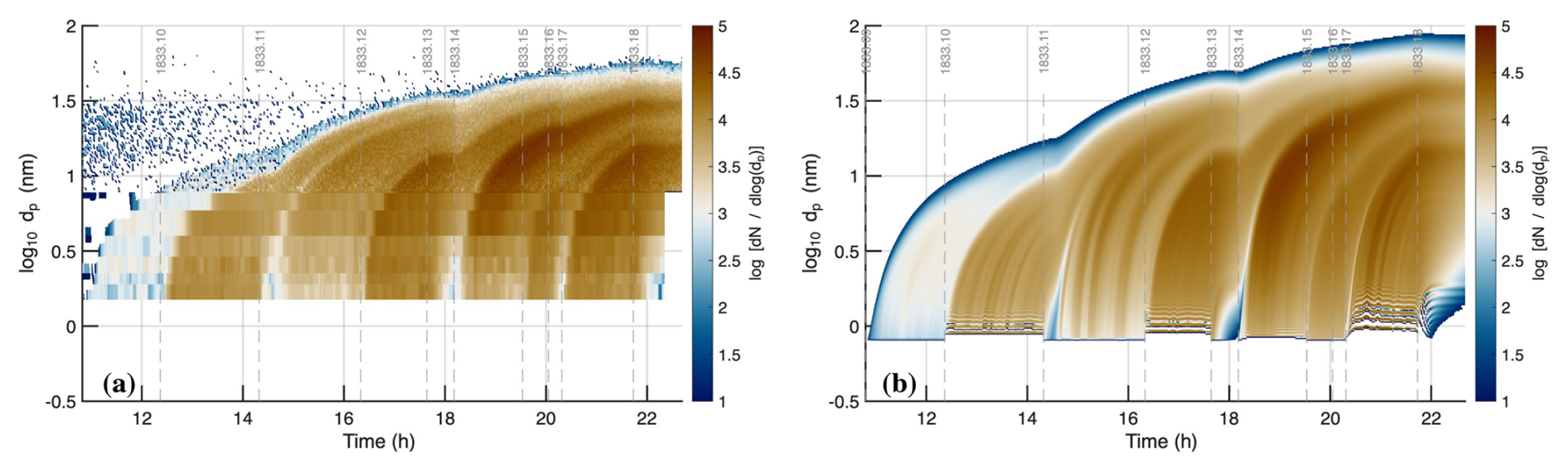
Figure 10 Observed (a) and modeled (b) particle size distribution during the UVX stages of Run 1833 with optimized parameters. These include a factor of 1.15 scaling of H₂SO₄ and empirical nucleation rates, as well as hygroscopic growth of wet $({\mathrm{NH}}_{\mathrm{4}}{)}_{\mathrm{2}}-{\mathrm{SO}}_{\mathrm{4}}-({\mathrm{H}}_{\mathrm{2}}\mathrm{O}{)}_n$. Essentially all the features of the observations are reproduced by the simulation with good fidelity, including the timing, intensity, growth rate, and final size of the nucleation bursts during each stage.

Overall, we find excellent agreement with the observations after only modest (15 %) adjustment in the H₂SO₄ calibration assuming the growing particles are wet and the size distribution measurement is accurate. A larger Hamaker constant would enhance growth, but it would also lower the H₂SO₄ lifetime, which we have already constrained (though a full optimization would certainly show co-variance here). However, significant Van der Waals attraction is essential for the overall appearance of the size distribution – the sharply dropping growth rates vs. size shown in Fig. 5a are crucial for the emergence of sharp modes even with constant nucleation and growth, as a constant flux vs. size will form modes via condensational narrowing.

7.3.2 Nucleation coefficients

Our objective here is not to directly test the nucleation parameterization, but it is essential for modeled nucleation to reproduce the observed particle number in order to then use the dual constraint of overall particle size (i.e. growth rate) and condensation sink (i.e. surface area and number). Consequently, we specify (and adjust) nucleation coefficients as described in Sect. 7.1 for the broad ranges of H₂SO₄ corresponding to each light intensity step. We are able to reproduce the overall particle number distribution, confirming that the particle formation is roughly third-order in H₂SO₄ and first-order in ions as expected. For $c_{{\mathrm{H}}_{\mathrm{2}}{\mathrm{SO}}_{\mathrm{4}}}\simeq \mathrm{6}\times {\mathrm{10}}^{\mathrm{7}}$ cm⁻³, we find $k_{\mathrm{neut}}\simeq \mathrm{1.6}\times {\mathrm{10}}^{-\mathrm{33}}$ cm¹² s⁻³ and $k_{\mathrm{ion}}\simeq \mathrm{8.5}\times {\mathrm{10}}^{-\mathrm{36}}$ cm¹⁵ s⁻³. With calibrations like this one in place for each relevant CLOUD campaign, we will be able to re-evaluate the overall H₂SO₄ nucleation parameterizations in a comprehensive analysis that is well beyond the scope of this work.

Figure 3 shows that, while the AIS data during ion-induced nucleation show large depletion of negatively charged primary ions, they also show some depletion of positively charged primary ions. Indeed, at high NH₃ concentrations, ion-induced nucleation of H₂SO₄−NH₃ is known to proceed with both positive and negative ions (Kirkby et al., 2011). A model incorporating primary ion losses is required to explore this further, which we incorporate into our gas-phase kinetic simulation. Based on that model (discussed below) we conclude that negative nucleation is 90 % of the ion-induced pathway and positive nucleation comprises the remaining 10 %. With these coefficients, both the growth (constraining H₂SO₄) and the total particle number (constraining nucleation) are simulated with good fidelity as shown in Fig. 10.

Figure 11 shows observed and modeled size distributions at roughly 5.1 h during stage 06 (the high light intensity charged stage). The data show clear signs of three modes, with minima at d_p≃9 nm and d_p≃20 nm. There is a hint of a maximum at 5 nm (this is the burst from stage 06 itself), a major maximum at 17 nm (this is the intense burst from the neutral stage 05) and a final maximum at 23 nm (from stage 04, with the stage 03 burst along its leading edge). The simulations also shows these features, with a much clearer maximum near 5 nm, the main 17 nm mode and a shoulder near 23 nm. In the simulation the larger two modes have merged due to numerical diffusion, but the corresponding features over time in Fig. 10 are clearly evident.

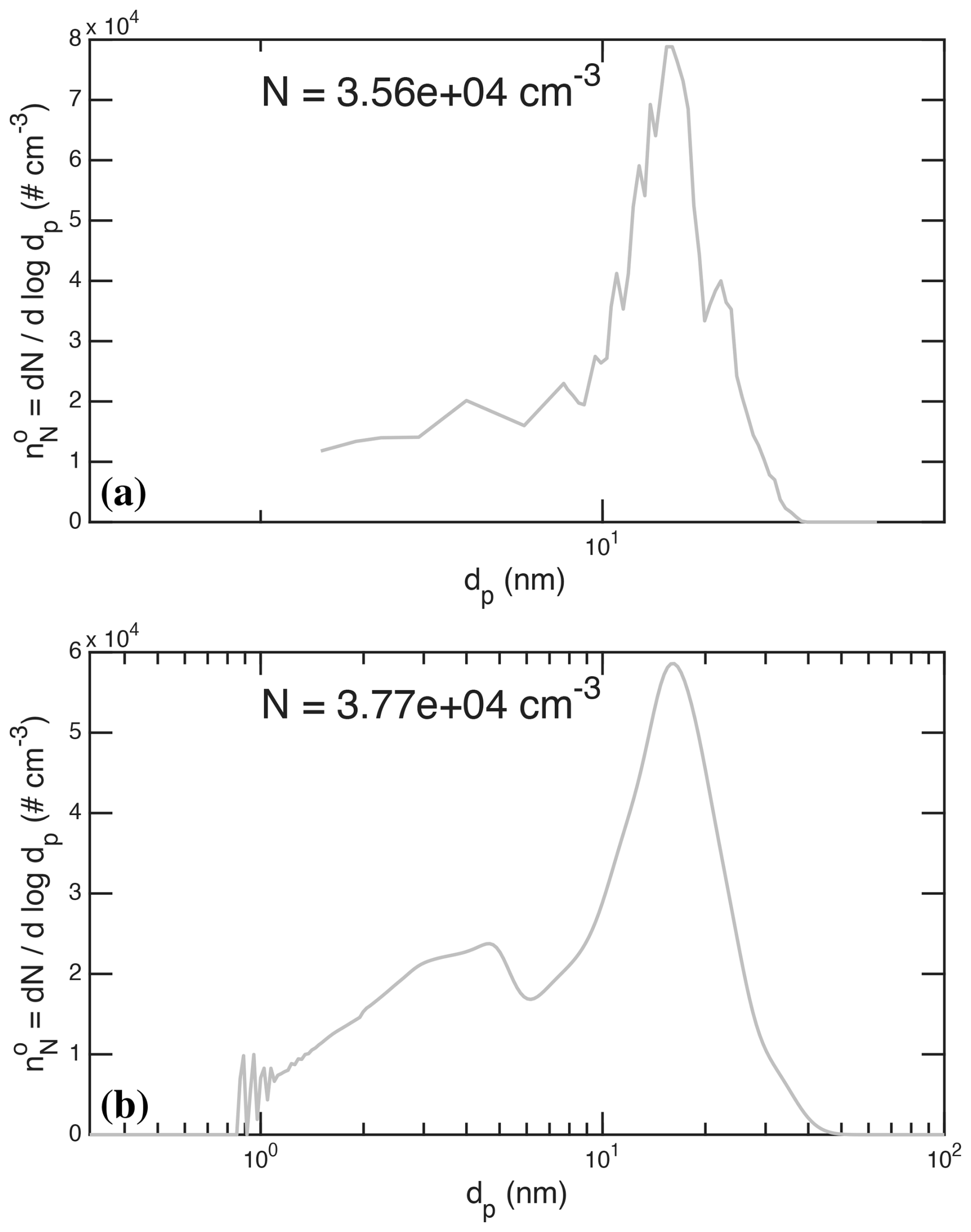
Figure 11 Comparison of measured and simulated size distributions near 5 h during stage 06. (a) Measured size distribution, combining DMA train and scaled SMPS values, with suspended surface area $S_p=\mathrm{2.3}\times {\mathrm{10}}^{-\mathrm{5}}$ m² m⁻³. (b) Simulated size distribution with the optimized parameters described here, with suspended surface area $S_p=\mathrm{2.5}\times {\mathrm{10}}^{-\mathrm{5}}$ m² m⁻³. Features of 3 distinct modes are evident in the observations and simulation, at the appropriate particle diameters. The steady increase in particles with increasing size for $\mathrm{1}<d_{\mathrm{p}}<\mathrm{5}\mathrm{nm}$ reflects nearly steady nucleation and growth flux ($J_{d_{\mathrm{p}}}$) because of the condensational narrowing associated with the declining collision speed associated with the Van der Walls effect on the collision cross section.

A final feature in Fig. 11 is the steady increase in the size distribution for $\mathrm{1}<d_{\mathrm{p}}<\mathrm{5}\mathrm{nm}$. This is caused by condensational narrowing at a steady nucleation rate and growth flux, $J_{d_{\mathrm{p}}}$ over this size range. This would not emerge without the decreasing condensation speed with size shown in Fig. 5. Largely because of the (diminishing) Van der Waals enhancement, the condensation speed decreases with size and so the number distribution must increase to compensate and keep the overall growth flux constant (in the absence of losses). This is condensational narrowing. Without these effects, simulations predict a much flatter distribution during constant nucleation rate simulations. Only coagulation would erode the smaller particles, and coagulation is a secondary contributor under these conditions.

7.4 Implications of microphysical calibration

Our findings based on the particle microphysics are quantitatively consistent with those of Stolzenburg et al. (2020). Specifically, we find that we can reproduce CLOUD observations of particle growth governed by H₂SO₄ condensation using a Van der Waals enhancement for that H₂SO₄ condensation of $\mathrm{6}\times {\mathrm{10}}^{-\mathrm{20}}$ J, which is slightly higher than the $\mathrm{4}\times {\mathrm{10}}^{-\mathrm{20}}$ J used in that work. We do find best agreement with an H₂SO₄ calibration factor of 1.2, but this is within error of the Stolzenburg et al. (2020) analysis as well as the very difficult H₂SO₄ calibration itself (Kürten et al., 2012). However, this is contingent on the growing particles containing considerable water, with a volume growth factor of 1.6, consistent with the deliquescence branch of ammonium sulfate, even though RH never exceeded the deliquescence relative humidity of ammonium sulfate. This is also consistent with the findings of Stolzenburg et al. (2020), who reported no dependence of growth rates on NH₃ under identical conditions.

8 Gas-phase Photochemistry

We now turn to gas-phase behavior of H₂SO₄ – this is almost the only connecting point between the particle (microphysical) constraints and the gas-phase photochemical constraints, including the desired photolysis actinometry. Once the absolute H₂SO₄ calibration is constrained, then it is possible to peel back the layers to calibrate the photolysis rates and light amplitudes. The original purpose of Run 1833 was light calibration – to use accurately measured H₂SO₄ along with precisely measured amplitudes from several light sources to determine the calibration factors for the volume averaged actinic flux of each light in CLOUD.

Photolysis drives a nominal set of reactions that produce H₂SO₄

$$\begin{array}{c}{\displaystyle }{\mathrm{O}}_{\mathrm{3}}\stackrel{h\mathit{\nu }}{⟶}\mathrm{O}{(}^{\mathrm{1}}\mathrm{D})+{\mathrm{O}}_{\mathrm{2}}(\mathit{\lambda }\lesssim \mathrm{320}\mathrm{nm})\\ {\displaystyle }\mathrm{O}{(}^{\mathrm{1}}\mathrm{D})+{\mathrm{H}}_{\mathrm{2}}\mathrm{O}⟶\mathrm{2}\mathrm{OH}\\ {\displaystyle }\mathrm{OH}+\mathrm{CO}\stackrel{{\mathrm{O}}_{\mathrm{2}}}{⟶}{\mathrm{HO}}_{\mathrm{2}}+{\mathrm{CO}}_{\mathrm{2}}\\ {\displaystyle }\mathrm{OH}+{\mathrm{SO}}_{\mathrm{2}}\stackrel{{\mathrm{H}}_{\mathrm{2}}\mathrm{O},{\mathrm{O}}_{\mathrm{2}}}{⟶}{\mathrm{H}}_{\mathrm{2}}{\mathrm{SO}}_{\mathrm{4}}+{\mathrm{HO}}_{\mathrm{2}}\end{array}$$

The production, $P_{{\mathrm{H}}_{\mathrm{2}}{\mathrm{SO}}_{\mathrm{4}}}$, is really a complicated function of the light amplitude comprising a photochemical box model, with production by design largely from OH+SO₂ and OH in turn largely produced by O₃ photolysis. The absolute light calibration factors also scale almost linearly with the (estimated) CO, which is the major OH sink. We have already tightly constrained the first-order H₂SO₄ loss terms, and here the calibrated condensation sink discussed above is used in the photochemical model via an interpolant.

In CLOUD, both O₃ and SO₂ are maintained by adding a steady flow into the continuously stirred reactor, and the resulting mixing ratios are shown in Fig. 4. While these are fairly stable, there is obvious variability that is also evidently associated with changes in light intensity. The ozone mixing ratio rises by more than 10 % during stages 01–06 as the Hg−Xe lamps approach full intensity, before relaxing back during the dark wall-loss and cleaning stages (07 and 08). It also declines modestly during stage 20 when the 385 nm LEDs are on at full power. The SO₂ mixing ratio drops by roughly 10 % during stages 01–06 but declines by more than 30 % during stage 20, reaching a steady state in a timescale similar to the wall-loss timescale for H₂SO₄.

The full photochemistry used for HO_x calibration to constrain $j_{\mathrm{O}{(}^{\mathrm{1}}\mathrm{D})}$ is listed in the Supplement. The key reactions first establish a steady state of O(¹D), with $c_{\mathrm{M}}=c_{{\mathrm{N}}_{\mathrm{2}}}+c_{{\mathrm{O}}_{\mathrm{2}}}$ and quenching rate coefficient k_q (actually slightly different for N₂ and O₂):

$$c_{\mathrm{O}{(}^{\mathrm{1}}\mathrm{D})}^{\mathrm{ss}}=\underset{P_{\mathrm{O}{(}^{\mathrm{1}}\mathrm{D})}}{\underbrace{j_{\mathrm{O}{(}^{\mathrm{1}}\mathrm{D})}{c}_{{\mathrm{O}}_{\mathrm{3}}}}}\underset{{\mathit{\tau }}_{\mathrm{O}{(}^{\mathrm{1}}\mathrm{D})}}{\underbrace{{\left(k_{\mathrm{q}}{c}_{\mathrm{M}}+k_{{\mathrm{H}}_{\mathrm{2}}\mathrm{O}}{c}_{{\mathrm{H}}_{\mathrm{2}}\mathrm{O}}\right)}^{-\mathrm{1}}}}$$

Because the H₂O reaction rate coefficient is gas kinetic but the quenching coefficients are roughly one in ten collisions, when the water vapor mixing ratio is about 0.01 (typical of room temperature and 50 % RH), about 10 % of the O(¹D) is converted to OH. This in turn establishes an OH steady state within roughly 1 s:

$$\begin{array}{c}{\displaystyle }{c}_{\mathrm{OH}}^{\mathrm{ss}}=\left(\mathrm{2}{k}_{\mathrm{O}{(}^{\mathrm{1}}\mathrm{D})}{c}_{{\mathrm{H}}_{\mathrm{2}}\mathrm{O}}{c}_{\mathrm{O}{(}^{\mathrm{1}}\mathrm{D})}\right){\mathit{\tau }}_{\mathrm{OH}}\\ {\displaystyle }{\mathit{\tau }}_{\mathrm{OH}}={\left(k_{\mathrm{CO}}{c}_{\mathrm{CO}}+k_{{\mathrm{O}}_{\mathrm{3}}}{c}_{{\mathrm{O}}_{\mathrm{3}}}+k_{{\mathrm{SO}}_{\mathrm{2}}}{c}_{{\mathrm{SO}}_{\mathrm{2}}}+\mathrm{\dots }\right)}^{-\mathrm{1}}\end{array}$$

The predominant OH sink is CO, with a few percent reacting with SO₂. Finally, this produces H₂SO₄, with a steady state established in at most the wall timescale (of order 10 min):

$$\begin{array}{c}{\displaystyle }{c}_{{\mathrm{H}}_{\mathrm{2}}{\mathrm{SO}}_{\mathrm{4}}}^{\mathrm{ss}}=\left(k_{{\mathrm{SO}}_{\mathrm{2}}}{c}_{{\mathrm{SO}}_{\mathrm{2}}}{c}_{\mathrm{OH}}\right){\mathit{\tau }}_{{\mathrm{H}}_{\mathrm{2}}{\mathrm{SO}}_{\mathrm{4}}}\\ {\displaystyle }{\mathit{\tau }}_{{\mathrm{H}}_{\mathrm{2}}{\mathrm{SO}}_{\mathrm{4}}}={\left(k_{{\mathrm{H}}_{\mathrm{2}}{\mathrm{SO}}_{\mathrm{4}}}^{\mathrm{wall}}+k_{{\mathrm{H}}_{\mathrm{2}}{\mathrm{SO}}_{\mathrm{4}}}^{\mathrm{cond}}+\mathrm{\dots }\right)}^{-\mathrm{1}}\end{array}$$

Overall, the fraction of O₃ photolysis toward O(¹D) that forms H₂SO₄ is only a few per mil.

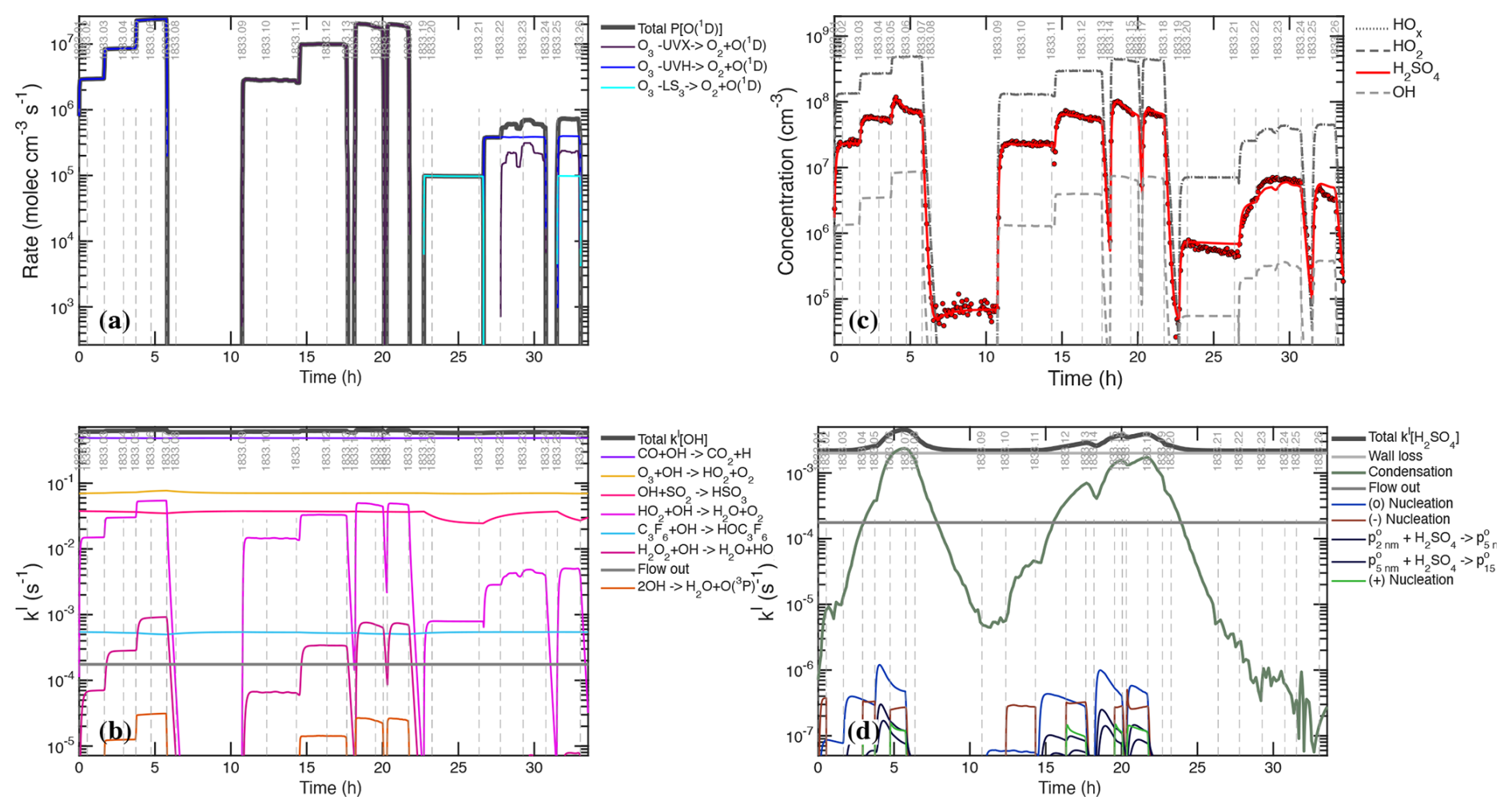
Figure 12 Actinometry calibration, with production and loss terms associated with H₂SO₄ based on corrected H₂SO₄ (${\mathcal{F}}_{{\mathrm{H}}_{\mathrm{2}}{\mathrm{SO}}_{\mathrm{4}}}^{\mathrm{cal}}=\mathrm{1.1}$). (a) Primary, calibrated photolysis rates producing O(¹D) from 3 different light sources. (b) Contributions to the OH first-order loss (lifetime). (c) Measured and modeled H₂SO₄ (with modeled HO₂ and OH, where ${\mathrm{HO}}_x={\mathrm{HO}}_{\mathrm{2}}+\mathrm{OH}$ is essentially coincident with HO₂); (d) Contributions to the H₂SO₄ first-order loss (lifetime). Photolysis rates are calibrated based on the smoothed light amplitudes shown here, with calibration coefficients adjusted to give optimal agreement with H₂SO₄. The H₂SO₄ behavior is reproduced with excellent fidelity, including timing and amplitude of depletion associated with the increased condensation sink, which is clearly evident in the H₂SO₄ lifetime as well. This in turn means the average OH concentration is known, and from OH loss, the balanced production constrains O(¹D) production from O₃ photolysis.

Figure 12 shows the major contributing processes to gas-phase closure throughout Run 1833. This includes O(¹D) production tied to measured light amplitudes, the OH lifetime, the H₂SO₄ simulated and measured concentrations (along with simulated HO₂ and OH) and finally the H₂SO₄ lifetime. With the first-order loss of H₂SO₄ well constrained, the absolute H₂SO₄ concentration in Fig. 12 is scaled by ${\mathcal{F}}_{{\mathrm{H}}_{\mathrm{2}}{\mathrm{SO}}_{\mathrm{4}}}^{\mathrm{cal}}=\mathrm{1.15}$. Almost all features of the H₂SO₄ time trace are reproduced with good fidelity, including the downturn in stage 05 (both the timing and amplitude) and the undershoot from the (unknown) dark H₂SO₄ source in stage 08 (which we simulate as a constant flow). That undershoot is caused by extra loss – a residual condensation sink from suspended particles. For the full span of stages 01–19, the model-measurement agreement is well within 10 %, giving us high confidence in the overall constraints (including the precision of the measured light amplitudes, O₃, and SO₂). This leaves only a single scaling factor common to all light sources to accurately constrain $j_{\mathrm{O}{(}^{\mathrm{1}}\mathrm{D})}$.

The less precise agreement after stage 19 (but still for the most part within 20 %) is at lower H₂SO₄ with more complicated stages; stage 20 is a cleaning stage with the 385 nm LEDs (LS1) illuminated and concurrent wall loss of SO₂ and O₃ as well as non-trivial condensation, stages 21–23 include very low excimer intensity with noisy amplitudes despite the median smoothing, and stage 25 again has declining SO₂ and significant excimer contributions. As there is little model-measurement bias, the 20 % deviations are attributable to noise. Because the H₂SO₄ is the only significant connection between the gas-phase photochemistry and the particle microphysics, the very high fidelity of this model-measurement agreement (after H₂SO₄ calibration) effectively decouples the microphysical and photochemical models, though the photochemistry (because of the H₂SO₄ condensation loss) remains dependent on accurate constraints from the microphysics.

There is no evidence for “hidden sulfuric acid”; there is nowhere to hide. The precise agreement between simulated and observed H₂SO₄ over at least a factor of 10 as light intensities change confirms this. A primary indicator for unobserved H₂SO₄ contained in small clusters of NH₄⋅HSO₄ would be nonlinear observed H₂SO₄ with increasing absolute H₂SO₄, as the clusters concentrations are at least quadratic in H₂SO₄ (Rondo et al., 2016). The relatively low nucleation rate coefficients, far below the kinetic limit, also confirm that small clusters are an inconsequential reservoir of H₂SO₄. Small clusters sequester a substantial pool of H₂SO₄ when nucleation is near the kinetic limit, such as with the H₂SO₄+(CH₃)₂NH system (Lehtipalo et al., 2016), but not here.

In addition to the principal photolysis of ${\mathrm{O}}_{\mathrm{3}}\stackrel{\mathrm{h}\mathit{\nu }}{⟶}\mathrm{O}{(}^{\mathrm{1}}\mathrm{D})+{\mathrm{O}}_{\mathrm{2}}$, the effects of two other photolysis processes are evident in Fig. 13. The Hg−Xe lights produce sufficient fluence for λ<250 nm to drive weak photolysis of molecular oxygen, ${\mathrm{O}}_{\mathrm{2}}\stackrel{\mathrm{h}\mathit{\nu }}{⟶}\mathrm{2}\mathrm{O}{(}^{\mathrm{3}}\mathrm{P})$, but also there is clear evidence that especially the 385 nm LED (on at full intensity in stages 19–20 and again in stage 25) drives what appears to be stoichiometric (1 : 1) loss of SO₂ and O₃. The SO₂ reaches a new, steady state level roughly one-third lower than its initial value, which under dark conditions is governed by the flow in and the chamber ventilation timescale (1.7 h). We conclude that this loss is a photon mediated reactive wall uptake of SO₂+O₃, with at least the sulfur containing reaction products (presumably SO₄) remaining on the wall. It is possible that the H₂SO₄ observed during stage 20 indicates small evaporation of H₂SO₄ from this (copious) wall source, but it is also possible that there is sufficient overlap between the high-frequency tail of the light source and O₃ absorption to produce some OH; separating these possibilities would require direct HO_x measurement. However, this source is a factor of 10–100 weaker than the targeted UV sources (UVH and UVX) even with the high 385 nm LED intensity. Consequently, we conclude that it is insignificant to the overall calibration.

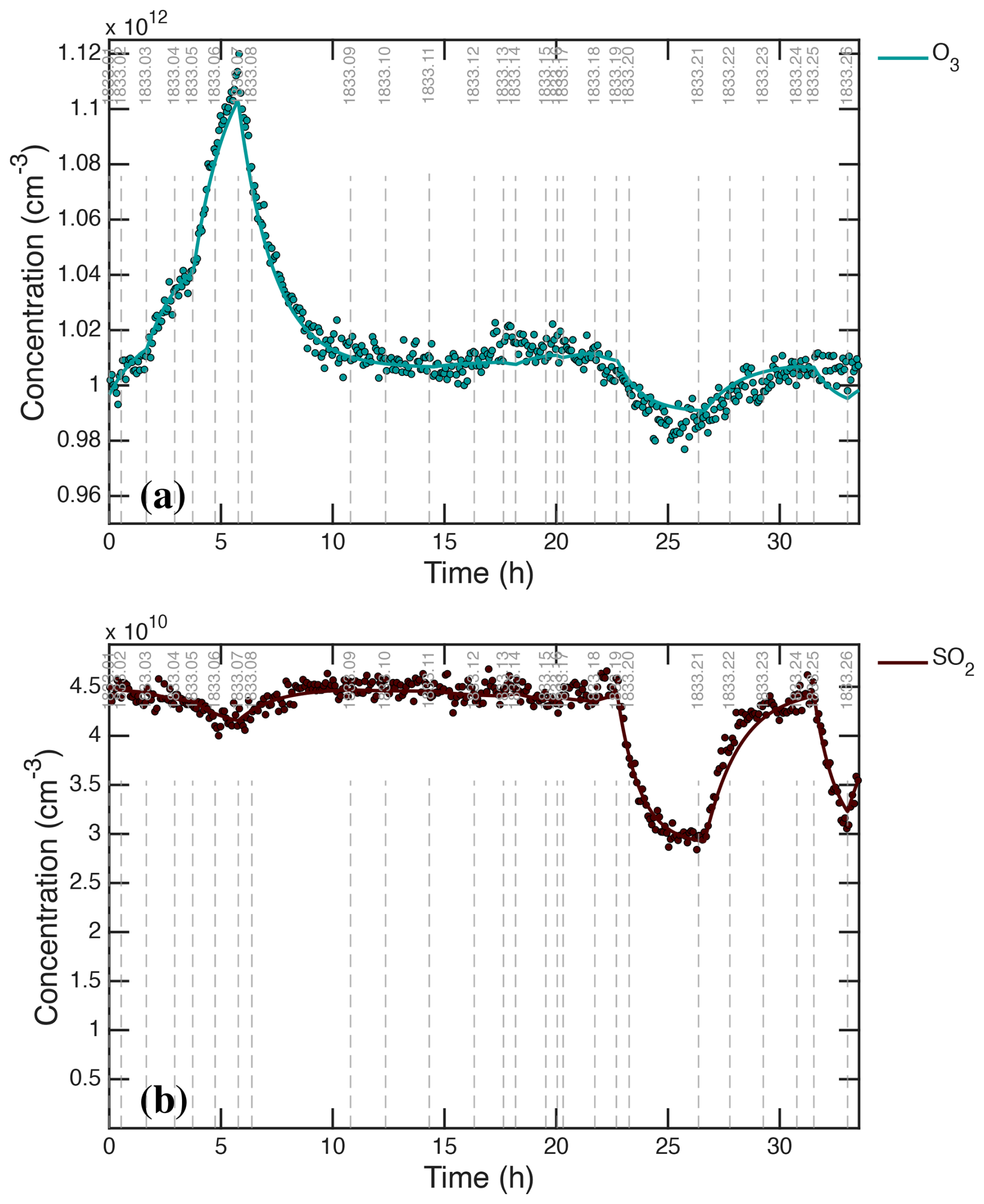
Figure 13 Simulated (curve) and observed (points) gas-phase precursors with smoothed and interpolated measurements. (a) O₃. (b) SO₂. Note the different, linear y-axis scales compared to Fig. 4. Observed values have been smoothed with a median filter and interpolated to model time points as needed. Production of O₃ via O₂ photolysis during the Hg−Xe (UVH) stages is evident, as is a stoichiometric (1 : 1) decrease in both O₃ and SO₂ especially with 380 nm LED (LS1) illumination after stage 19 but also with UVH illumination before stage 08.

Comparing Figs. 12 and 13 with Figs. 2 and 4, the importance of smoothing via median filtering (and excluding UVX crosstalk from the UVH amplitudes) is also clear. Many of the finer features in the model values are impossible to see in the unfiltered raw data. Even with the increased precision of the smoothing, a model for dry growth is equally precise, with twice the H₂SO₄; this agreement does not differentiate between the dry growth and wet growth scenarios (changing the H₂SO₄ calibration simply shifts the y-axis scale). This is because the HO_x chemistry (production and loss) is nearly linear over the conditions of this run, with the OH+HO₂ reaction reaching at most 10 % of the overall OH loss in Fig. 12b.

9 Charge and Ion Production and Loss

Close examination of the CPC_2.5 data in Fig. 6 shows the effect of voltage transitions in the clearing field removing charged particles – for example the particle number drops by roughly 20 % at the start of stage 05 (a neutral nucleation state at full UVH power) and by less than 10 % at the start of stage 02 (also a neutral nucleation stage, at 20 % UVH power). This indicates that only a small fraction of the particles in stage 01 were charged by the end of the stage, even though this is an ion induced nucleation (charged) stage with evidently much more particle formation than the subsequent neutral stage. The same applies at the end of the gcr stage 04 less than 20 % of the particles were charged (though notably more than after stage 01). That is confirmed by Fig. 3. The sectional particle microphysics model presented so far neglects charge, and thus we have so far left out of our model-measurement constraints are the primary ions and charged particles. These, especially the primary ions, are much closer in size and collision dynamics to the gas-phase than the particle microphysics, and so we incorporate them into our gas-phase photochemical model, with primary ion production as well as loss via wall deposition (including the clearing field), ion recombination, and diffusion charging (and neutralization) of larger particles.

9.1 Modal scheme

To simulate the loss of primary ions we need some treatment of the number and charge state of larger particles (the overall condensation sink), so we simulate nucleation and growth in the gas-phase model with a succession of pseudo-reactions in a simplified modal representation of particles with nominal diameters d_p=2, 5, and 15  nm, and charge $q=-\mathrm{1}$, 0, +1, labeled $p_{d_{\mathrm{p}}}^q$. Along with the primary ions, we refer to the 2 nm mode as clusters, the 5 nm mode as the nucleation mode, and the 15 nm mode as the Aitken mode. Nucleation is formation of the 2 nm cluster mode (in any charge state) and we assume that growth to the 5 nm mode is required for detection in the CPC_2.5. The scheme is designed to be accurate for ions and the nucleation rates, and “reasonable” for the larger particles. This is not a formal modal scheme with mode widths or any representation of composition, just charge. Our objective here is to use this portion of the model to identify the major processes controlling the charged microphysics and charge balance in the experiment.

As always the scheme starts with nucleation. Here this forms the first mode, nominally 2 nm clusters, followed by condensational growth from mode to mode.

$$\begin{array}{c}{\displaystyle }\mathrm{3}{\mathrm{H}}_{\mathrm{2}}{\mathrm{SO}}_{\mathrm{4}}+{\mathrm{NH}}_{\mathrm{3}}(+n^{\pm })⟶p_{\mathrm{2}}^{\circ ,\pm }\\ {\displaystyle }{\mathrm{H}}_{\mathrm{2}}{\mathrm{SO}}_{\mathrm{4}}+p_{\mathrm{2}}^{\circ ,\pm }⟶p_{\mathrm{5}}^{\circ ,\pm }\\ {\displaystyle }{\mathrm{H}}_{\mathrm{2}}{\mathrm{SO}}_{\mathrm{4}}+p_{\mathrm{5}}^{\circ ,\pm }⟶p_{\mathrm{15}}^{\circ ,\pm }\end{array}$$

The nucleation coefficients are identical to those in the microphysical model, but the ions are treated explicitly. We model growth as first-order and rate-limited by H₂SO₄ with a rate coefficient to drive growth from one mode to the next.

$$\begin{array}{c}{\displaystyle }{\mathrm{H}}_{\mathrm{2}}{\mathrm{SO}}_{\mathrm{4}}+p_{\mathrm{2}}^{\circ ,\pm }\stackrel{k_{\mathrm{grow}}^{\mathrm{2}}}{⟶}{p}_{\mathrm{5}}^{\circ ,\pm }\\ {\displaystyle }{\mathrm{H}}_{\mathrm{2}}{\mathrm{SO}}_{\mathrm{4}}+p_{\mathrm{5}}^{\circ ,\pm }\stackrel{k_{\mathrm{grow}}^{\mathrm{5}}}{⟶}{p}_{\mathrm{15}}^{\circ ,\pm }\end{array}$$

However, it takes several hundred H₂SO₄ collisions to grow from 2 to 5 to 15 nm. That number for each case is $g_{{\mathrm{H}}_{\mathrm{2}}{\mathrm{SO}}_{\mathrm{4}}}^{d_{\mathrm{p}}}\gtrsim \mathrm{100}$, and so the effective modal growth coefficient is

$$k_{\mathrm{grow}}^{d_{\mathrm{p}}}=k^{d_{\mathrm{p}}}/g_{{\mathrm{H}}_{\mathrm{2}}{\mathrm{SO}}_{\mathrm{4}}}^{d_{\mathrm{p}}}<{\mathrm{10}}^{-\mathrm{12}}{\mathrm{cm}}^{-\mathrm{3}}{\mathrm{s}}^{-\mathrm{1}}$$

where $k^{d_{\mathrm{p}}}$ is the collision kernel for single collisions of H₂SO₄ with particles of size d_p. The rate coefficient includes the growth enhancements by co-condensation of NH₃ and hygroscopic growth if appropriate. The apparent loss of H₂SO₄ from this modal growth is trivial compared with the (observationally constrained) condensation sink term of H₂SO₄ itself; that is a significant advantage as it effectively decouples the H₂SO₄ loss from the particle formation and growth in the mechanism, allowing us to continue to constrain H₂SO₄ loss by the observed condensation sink while simultaneously modeling the nucleation and growth via this modal mechanism.

Importantly, we also represent diffusion charging. At these particle sizes, essentially no particles are doubly charged, but charging and neutralization are important.

$$\begin{array}{c}{\displaystyle }{p}_{d_{\mathrm{p}}}^{\circ ,\pm }+n^{\mp }⟶p_{d_{\mathrm{p}}}^{\mp ,\circ }\\ {\displaystyle }{p}_{\mathrm{5},\mathrm{15}}^{\circ ,\pm }+p_{\mathrm{2}}^{\mp }⟶p_{\mathrm{5},\mathrm{15}}^{\mp ,\circ }\\ {\displaystyle }{p}_{\mathrm{15}}^{\circ ,\pm }+p_{\mathrm{5}}^{\mp }⟶p_{\mathrm{15}}^{\mp ,\circ }\end{array}$$

The charging occurs via collisions of the primary ions themselves (n^±) but also via collisions involving any charged particles smaller than a given target particle (i.e. all collisions involving charge of 15 nm particles with any primary ions, 2 nm, or 5 nm particles). In this simplified modal mechanism, particle charging does not cause growth, and so it removes the smaller charge carrying particle (this is an important coagulation mechanism; Mahfouz and Donahue, 2021).

Coagulation also occurs via neutral collisions between particles of all sizes, which again does not cause growth in our (overly) simple scheme:

$$p_{\mathrm{2},\mathrm{5},\mathrm{15}}^{\circ }+p_{\mathrm{2},\mathrm{5},\mathrm{15}}^{\circ }⟶p_{\mathrm{2},\mathrm{5},\mathrm{15}}^{\circ }$$

Analysis of growth rates in the microphysical model below shows that, for the conditions of this experiment, condensational growth far exceeds coagulational growth and so these assumptions are warranted.

9.2 Model results

The gas-phase modal scheme as part of the photochemical model is substantially faster than the full sectional microphysical model (and would be vastly faster than a full sectional microphysical model treating charge). We show the results in Figs. 14 and 15. Figure 14 shows the modeled and measured primary ions, the 2 nm cluster mode for each charge state along with the total, and the total particles in the 5 nm nucleation and 15 nm Aitken modes along with the sum of these two modes (nominally N₅) and the observed CPC_2.5 count. Figure 15 shows the concentration in each mode for negatively and positively charged particles along with the total of all the modes (nominally $N_{\mathrm{2}}^{\pm }$). As with the microphysical model, and despite its simplifications, this modal simulation reproduces the observations with evident (to the eye) good fidelity.

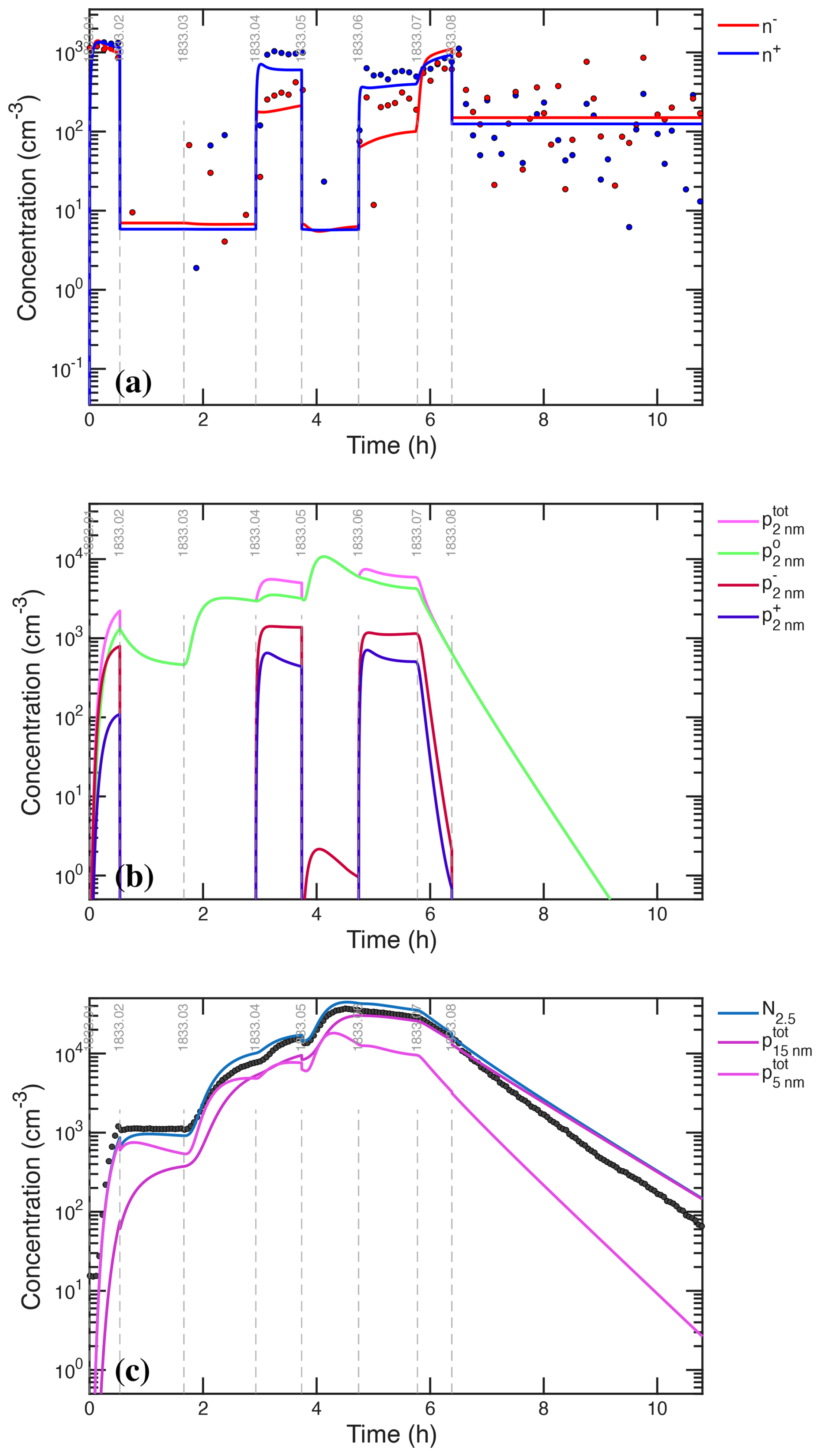
Figure 14 Simulation of particle evolution (including charge state) during the UVH stages using a modal scheme with primary ions and modes centered at 2, 5, and 15 nm along with relevant observations. (a) Simulated (red and blue curves) and observed (red and blue circles) primary ions. (b) Simulated concentration of the 2 nm mode, representing clusters of each charge state. (c) Simulated (blue curve) and observed (filled circles) N₅; the blue curve is the sum of magenta 5 and 15 nm particles. The primary ion simulation reproduces the observed depletion of primary ions, strongly biased toward negatively charged ions. The 2 nm clusters are principally neutral even during stages that are dominated by ion induced nucleation, such as stage 01, because the charged clusters are steadily neutralized by ion-ion recombination on a timescale of around 10 min. Finally, the simulated N₅ trace reasonably reproduces the CPC_2.5 observations, with similar fidelity to the microphysical model. Notably, the simulation reproduces the dips in particle numbers at the beginning of neutral stages immediately following charged stages, such as stage 05, when the charged particles are rapidly swept from the chamber as well as the loss rate of the largest particles during the cleaning stage (08) where charging and electrostatic removal enhances that loss.

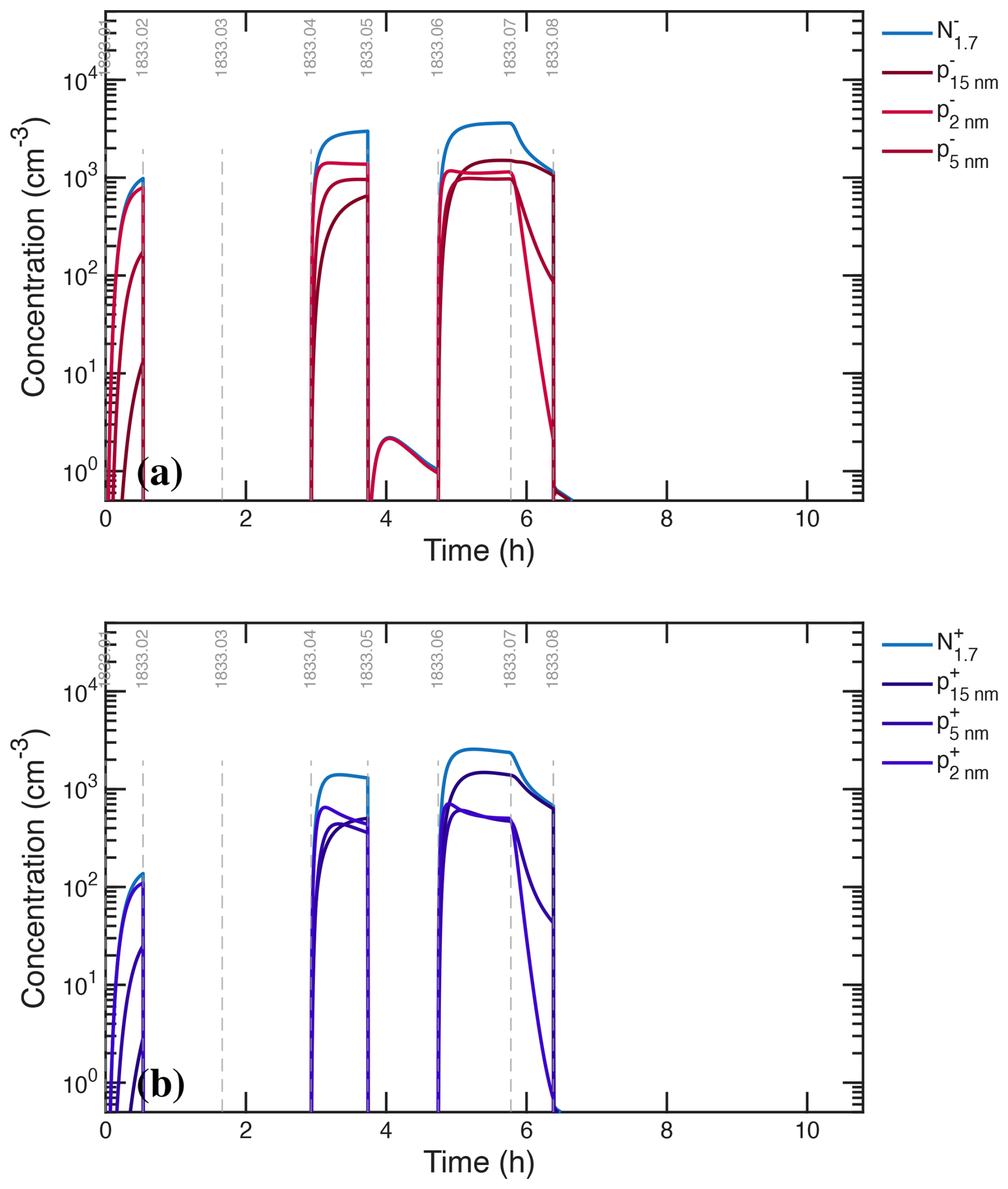
Figure 15 Simulated charged particles vs. time, with concentrations of each mode (centered at 2, 5, and 15 nm) as well as the sum, $N_{\mathrm{1.7}}^{\pm }$. (a) Negatively charged particles. (a) Positively charged particles. As with observations, during strong ion-induced nucleation stages (i.e. 06) there are 2–3 × 10³ cm⁻³ of both negatively and positively charged particles. Strong ion-induced nucleation yields slightly fewer positively charged than negatively charged particles, whereas weak ion-induced nucleation (i.e. stage 01) favors negatively charged particles by nearly an order of magnitude.

For the primary ions in Fig. 14a we subtracted an empirical background value of 200 cm⁻³ from each polarity since these represent the AIS instrument background signal for our operating conditions. With the AIS offset correction, the simulated ion concentrations match the observations reasonably well. The particle-free steady state near 1500 cm⁻³ confirms an ion-pair production rate of 7 cm⁻³ s⁻¹ (combining galactic cosmic rays with stray muons from the CERN Proton Synchrotron and external targets). The primary ions rarely reach 1500 cm⁻³ – only the weakest charged nucleation stages, such as stage 01, are free of ion depletion for either polarity. The ion depletion and the charge asymmetry are captured during strong ion-induced nucleation stages (04, 06). A simulation without a 10 % contribution from the positive ion channel does not reproduce the cation depletion.

Figure 14b shows that the neutral 2 nm particles comprise more than half of the total 2 nm mode at all times; the green neutral concentration is always either coincident with the magenta total or 10 %–20 % below it. During stage 01 the nucleation is more than 90 % ion induced, and even during that stage, the 2 nm clusters are mostly neutral, with a strong asymmetry between the negatively and positively charged particles. However, without the 10 % positively charged nucleation channel, the positively charged particle concentration during stage 01 would be far too low compared to Fig. 3; the observed asymmetry during that stage is a telling indicator of the relative intensity of the two polarities. Evidently, neutralization of the 2 nm negatively charged particles by positively charged primary ions, or positively charged clusters, is substantial.

Figure 14c shows the totals of the 5 nm nucleation and 15 nm Aitken modes and their sum (nominally N₅), along with the observed CPC_2.5 signal. Because this simulation has modes at 2 and 5 nm, comparison with the CPC_2.5 signal (d_p=2.2 nm) is imprecise. However, except for weak nucleation periods with substantial 2 nm particle concentrations, the sum of the two larger (nucleation and Aitken) modes from the simulation agrees with the observations to within 10 %. Notably, the simulation quantitatively reproduces the concentration dips when stages switch from charged to neutral (i.e. the clearing field is turned on, at the start of stage 05) and any charged particles are removed quickly.

Figure 15 shows that the concentrations of the three modes are almost always in rank order for the negatively charged particles during gcr stages. These are all represented with a crimson hue, with brighter colors corresponding to smaller modes. The smaller negatively charged particles are always more abundant, and the larger modes react to the onset of ion induced nucleation much more slowly than the smallest particles (e.g. stage 10). This is opposite to the thermodynamics of charging but consistent with nucleation and growth, with some losses. Below 10–15 nm, the principal reason the negatively charged particles exist is because they grew up from smaller negatively charged particles. During the wall loss stage, 07, the reverse is true; the source is removed and the smaller particles are lost before the less diffusive larger particles.

The positively charged particles present a more nuanced picture. At times, such as during stage 06, the larger positively charged particles are more abundant than the smaller modes, suggesting that diffusion charging and not nucleation and growth is the major source. This diffusion charging also depletes the smaller positively charged particles and so deprives the positively charged nucleation channel of its source. Overall, there is a direct relationship between the relative abundance of small charged particles below 10 nm diameter, compared to the neutral abundance, and the importance of ion induced nucleation of that polarity.

Treating the nucleation and growth with this modal simulation, along with the charge production and loss, ultimately yields a good simulation of the total primary ion behavior, including the asymmetry between positively and negatively charged ions, clusters and particles. Finally, the particle loss rates during the cleaning stage are adequately reproduced. Overall this thus yields the final element of closure when combined with the (sectional but uncharged) microphysical model and the gas-phase photochemistry.

10 Process Rates

A crucial element of both the microphysical and photochemical models is that they disaggregate and diagnose process rates. This is vital to understanding the results but also to experimental design – experiments are often designed to constrain or test a specific process, and the results of a given test are interpretable only if that process is actually prominent, making the observations sensitive to the process. Nonlinear interconnected systems such as this can be subtle – stiff systems almost by definition are sensitive to seemingly minor terms – but careful rate analysis is if anything more important in that case.

For the current system, both the microphysical and photochemical rates are important diagnostics. We have already presented several rate analyses in the process of showing the key model results.

10.1 Photochemical rates

In order to assess the H₂SO₄ loss we have already presented its production and loss rates during the UVH stages in Fig. 7, side by side with identical y-axis ranges. The plots include individual rate terms as well as totals. This format facilitates a quick assessment of the overall rate balance. The overall production increases sharply for the three UVH settings, while the loss rate catches up to the production rate asymptotically on a timescale that is evidently a small fraction of an hour. The same applies during the wall loss and cleaning stages (07 and 08), when the photochemical production drops quickly past the (unknown) chamber source, which is modeled as a steady flux of 280 cm⁻³ s⁻¹. After the induction period in each stage, production and loss clearly balance to give a steady state; however, the growing condensation sink clearly plays a role as it grows to compete with the wall loss term, even driving the small “undershoot” in the H₂SO₄ during the early part of the cleaning stage (08). It is also clear that photochemical production balances wall and condensation losses, with all other terms playing a minor role (though ventilation is important at the 10 % level).

Figure 8 shows the complementary assessment of the H₂SO₄ first-order loss during the UVH stages. This is a separate and equally important diagnostic. Here the emerging importance of condensation between stage 04 and the start of stage 08 is made clear, but also the quantitative lifetime of 500 s or less confirms the rapid but discernible approach to steady state of both $c_{{\mathrm{H}}_{\mathrm{2}}{\mathrm{SO}}_{\mathrm{4}}}$ and $L_{{\mathrm{H}}_{\mathrm{2}}{\mathrm{SO}}_{\mathrm{4}}}$.

Figure 12b also shows the contributions to the OH first-order loss, which in total is slightly slower than 1 s⁻¹. The largest sink is CO, followed by O₃, with SO₂ contributing at less than 10 %. All of these are fairly constant, though the dips in especially SO₂ are evident. Nonlinear processes such as HO₂+OH play a very modest role of at most a few percent. The limited role of SO₂ and especially the limited non-linear HO_x loss reactions are the main reason why the gas-phase photochemistry is almost insensitive to the absolute H₂SO₄ calibration beyond simply shifting the (log) y-axes. Doubling the H₂SO₄ requires doubling the OH which requires doubling the light intensity; beyond that, the shapes of the concentration profiles are nearly identical.

10.2 Charged modal microphysics

Interpretation of the H₂SO₄ rate and lifetime plots is relatively straightforward. Other important processes are more nuanced. Figure 16a shows the production and Fig. 16b the loss rates for negative primary ions (n⁻). The ions are almost always in steady state, and so the total production and loss balance; however, the very brief transients are evident at the start of neutral stages when the clearing field turns on suddenly and the loss rates show a brief spike. For stages 04 and 06, ion-induced nucleation is the predominant loss for the primary negatively charged ions and so the crimson “(–) nucleation” curve nearly reaches the total loss; this represents the saturated ion formation limit, but also means that the primary ions have all grown and are thus depleted. This in turn affects the particle charging dynamics and so particle losses. Even during stage 01, nucleation becomes competitive with ion recombination (“cluster neutralization”) and wall losses, which in turn are all nearly equal during the stage; this is the most complicated condition, where the three major loss mechanisms – recombination, wall loss (deposition) and nucleation – are all competitive and nearly equal.

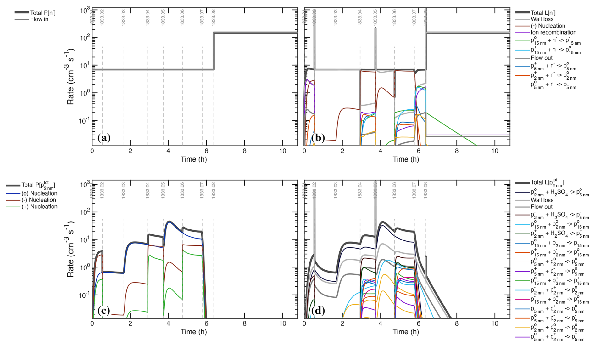
Figure 16 Production (P[x]) vs. loss (L[x]) for primary negative ions and the total 2 nm cluster mode from the gas-phase model. Both show production rates on the left and loss rates on the right, with identical scales to permit assessment of the rate balance. Transitions from charged to neutral stages (e.g. the beginning of stages 02 and 05) cause a short, sharp increase in loss as the clearing field rapidly removes charged particles and the rate balance is re-established in seconds. (a) Production and (b) Loss of negatively charged primary ions. Production is steady at 7 cm⁻³ s⁻¹ gcr ion-pair formation aside from enhanced formation of 150 cm⁻³ s⁻¹ via the CERN beam during the cleaning stage 08; this is modeled as a homogeneous flow and is labeled “Flow in”. Loss has many competing elements, including wall loss, ion induced nucleation, recombination with positively charged ions (and larger particles), and diffusion charging of larger neutral particles. Loss by nucleation saturates during gcr nucleation stages 04 and 06, where the red nucleation rate dominates the loss term. (c) Production and (d) Loss of total clusters (all charge states comprising the 2 nm particle mode). Production is nucleation, separating neutral (∘), negatively (−) and positively (+) charged clusters. Loss includes wall deposition but is predominantly growth to the larger (5 nm) mode. Numerous processes involving ions and charged particles of opposite polarity contribute during gcr stages (04 and 06).

An analysis of the primary ion first-order loss rates is also revealing, as shown in Fig. 17. The ion lifetimes are under 100 s, revealing why they are in steady state. The most notable feature is the modulation of the wall loss as the clearing field turns on and off, with the primary ion lifetimes dropping to 1 s when the clearing field is on. In contrast, nucleation depends only on (the third power of) $c_{{\mathrm{H}}_{\mathrm{2}}{\mathrm{SO}}_{\mathrm{4}}}$ and so becomes prominent during the medium and high intensity UVH stages. For the negative ions, these are the only notable sinks. For the weaker positive channel, nucleation never overwhelms other processes, and during stage 06 a host of neutralization channels are important secondary sinks. This plays a key role in the overall mechanism, as neutralization of the more intense negative ion induced nucleation pathway causes neutral particles to dominate the overall distribution, as we observe. However, the results suggest that for somewhat higher H₂SO₄, the positive nucleation would also saturate; this would have a secondary effect of reducing the neutralization rate by completely depleting the primary ions of both polarities.

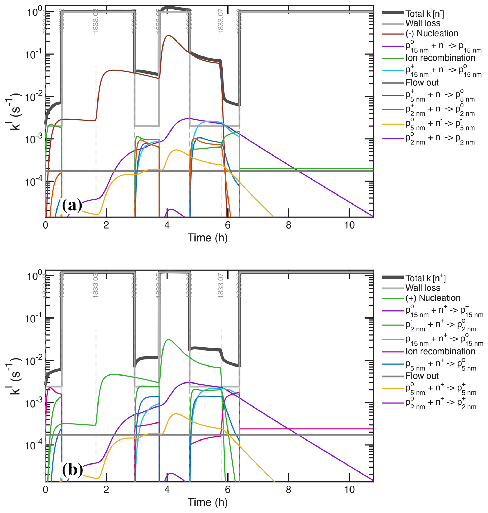
Figure 17 Simulated first-order loss during the UVH stages for (a) negatively charged and (b) positively charged primary ions. At the beginning of stage 01, without substantial nucleation or diffusion charging, ion recombination is (by chance) equal to wall loss. High-voltage clearing stages (02, 03, 05, 08) increase the wall-loss to 1 s⁻¹. Both nucleation and a large condensation sink causing diffusion charging and neutralization increase the loss. Saturation of ion-induced nucleation (e.g. negatively charged ions during stage 04 and 06) is indicated by nucleation dominating the loss. At steady state (e.g. nearly in stage 04) diffusion charging and neutralization nearly balance, as required.

Nucleation produces the 2 nm cluster mode, and Fig. 16c shows production and Fig. 16d loss of the total 2 nm cluster mode mode in all charge states (neutral, negatively charged, and positively charged; ${\mathrm{N}}_{\mathrm{2.0}}=n_{\mathrm{2}}^{\circ }+n_{\mathrm{2}}^{+}+n_{\mathrm{2}}^{-}$). The total rates are more rounded compared to the square-wave shape of the primary ion rates, but there are more contributions to both production and loss. The sources of this family comprise each of the three nucleation rates (neutral, negatively charged and positively charged). The sinks include wall loss and dilution (“flow out”), growth by condensation of all three charge states (“cluster growth”), and also various forms of coagulation.

For the nucleation source, during stage 01 this is almost entirely (negatively charged) ion-induced nucleation, but, for higher $c_{{\mathrm{H}}_{\mathrm{2}}{\mathrm{SO}}_{\mathrm{4}}}$, the charge saturates at the ion-pair formation rate of 7 cm⁻³ s⁻¹ and adds only incrementally to the total. During stage 06, H₂SO₄ is high enough that even the weaker positive nucleation reaches half of the positive ion production rate, but it does not quite saturate. This shows one important element of constraining both polarities of ion induced nucleation – even though the positive channel is roughly 10 % as efficient as the negative channel, it remains important near the ion pair saturation limit and this has knock on effects on particle charging and neutralization, as we shall see. Once the ion induced channels saturate, the neutral pathway (blue) predominates even during the gcr stages, such as stage 06.

The loss terms are marginally more involved. Neutral condensational growth to 5 nm (dark blue) is almost always the leading sink of the 2 nm particles (meaning the particle survival probability is high), though wall loss is more important at lower H₂SO₄ when growth is slower. The spikes in wall loss at the start of stages 02 and 04 drive the small dips in the overall number discussed above. During the gcr stages, growth of negatively charged particles (dark crimson) plays a secondary role, and ventilation is consistently about 10 % of the total loss. A host of other processes are minor sinks, especially during the gcr stages when the small clusters can diffusion charge larger (neutral) particles but also be lost via coagulation to larger positively charged particles.

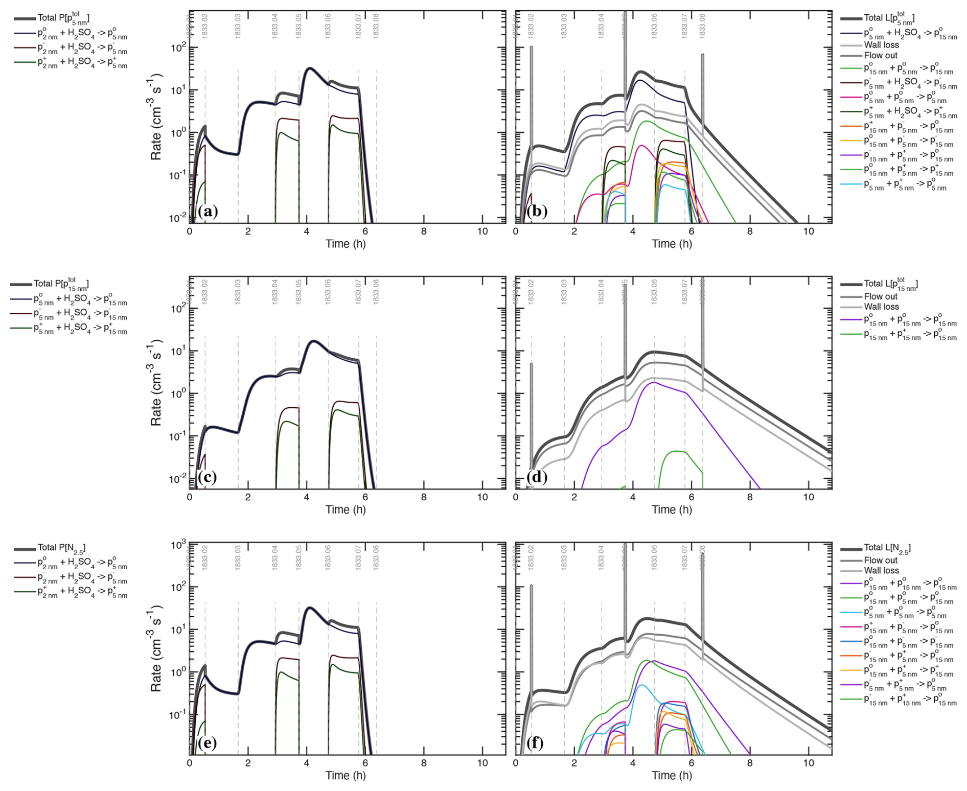
Figure 18 Production and loss of particle modes in the gas-phase model. (a) Production and (b) Loss of total 5 nm particles. Production is largely via neutral condensational growth from the 2 nm mode. Loss includes growth to 15 nm but also wall loss and ventilation loss, as well as coagulation between 5 and 15 nm modes during high-concentration stages 05 and 06. (c) Production and (d) Loss of total 15 nm particles. Production is almost exclusively neutral growth from the 5 nm mode. Loss includes ventilation and wall deposition with a 10 % contribution by coagulation during high concentration stages. (e) Production and (f) Loss of combined 5 and 15 nm particles (“𝒩₅”). Production is identical to the 5 nm production. Loss is split equally between wall deposition and ventilation, with three coagulation pathways between the two modes contributing during the high-concentration stages.

Figure 18 shows the production and loss terms for total particles (the sum of all charge states) for the larger particle modes at 5 nm (“nano”) and 15 nm (“Aitken”) as well as the total of those larger particles, which is identified by the family name “N_2.5”. The only source for these total mode families, within the scheme defined in the quasi-modal mechanism, is condensational growth.

Consequently, in Fig. 18a the production of nucleation-mode nano particles (p₅) is growth from the cluster mode (p₂), in each of the three charge states. Even at this size, neutral growth is always predominant even during gcr stages. Figure 18c shows that growth from p₅ to p₁₅ is qualitatively the same but the neutral pathway is almost completely dominant. As is typical, losses are more nuanced. In Fig. 18b for the 5 nm mode, growth to 15 nm, wall loss, and dilution (flow out) are all competitive, with growth becoming progressively more significant at high H₂SO₄ as expected. However, for the highest intensity UVH with high H₂SO₄ (stages 05 and 06), neutral coagulation loss of 5 nm nanoparticles to 15 nm Aitken mode particles comprises roughly 10 % of the overall nanoparticle loss rate. In Fig. 18d for the 15 nm mode, our simple scheme does not treat further growth, and flow out of the chamber takes over as the largest sink. However, neutral coagulation between 15 nm particles is also a 10 % sink.

Figure 18e shows production and Fig. 18f shows loss for the combination of the two modes (N_2.5). The production rates are identical to production for p₅ in Fig. 18a. However, nanoparticle growth from p₅ to p₁₅ is no longer a sink and coagulation between the two modes and coagulation among the 15 nm particles are roughly equivalent sinks, accounting for roughly 20 % of the total particle loss. Wall and ventilation losses are also roughly equal at 40 % each.

10.3 Microphysical process rates

The model with sectional microphysics permits more detailed simulation (and analysis) of the size-dependent microphysical processes, but it is not (yet) coupled to the gas-model and does not (yet) include charge. Consequently, it is driven by either observed or modeled vapor concentrations that drive nucleation and growth. As a reminder, this model uses (spherical equivalent) diameter, d_p, whereas instruments generally report mobility diameter, $d_{\mathrm{mob}}\simeq d_{\mathrm{p}}+\mathrm{0.3}$ nm (Larriba et al., 2011), so for example a 2.5 nm CPC has a physical cutoff diameter of d_p=2.2 nm.

Figure 19 shows the particle-phase rates at d_p=2.2 nm. Figure 19a shows J_2.2, which is the flux of particles across the 2.2 nm size cut in the sectional model. This includes both condensational growth as well as coagulation, but condensation constitutes the overwhelming majority of the flux; for growth involving “hidden” sulfuric acid clusters, the coagulation term would be much larger, as that is technically coagulation. An interesting feature is the drop in J_2.2 well after the end of stage 01, when the system switched from gcr to neutral conditions; this reflects the time delay due to growth between formation near 1 nm and appearance at 2.2 nm. This is similar to the slow drop of p₅ production in Fig. 18a.

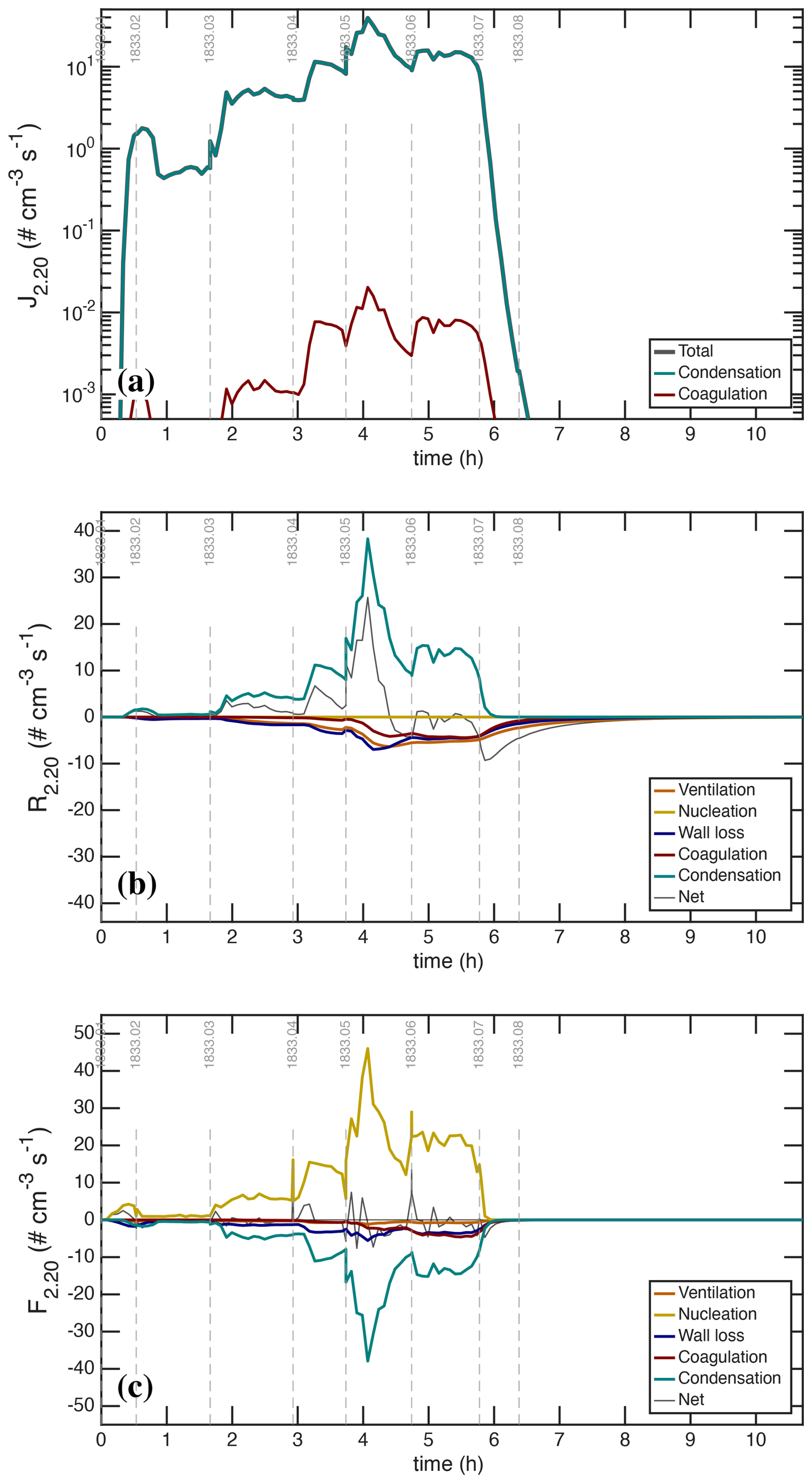
Figure 19 Rates in the sectional microphysical model at d_p=2.2 nm (d_mob≃2.5 nm). (a) Formation rate, J_2.2, defined as the flux of particles from d_p≤2.2 nm to d_p>2.2 nm. This is almost entirely due to condensation, but some coagulation contributes. (b) Integrated rates for all processes for d_p≥2.2 nm. Condensation is the source (matching panel a) as particles nucleate at d_p=0.8 nm and grow into the N_2.2 range, whereas losses are distributed more or less evenly among wall loss, ventilation (dilution), and coagulation. These are the critical loss terms needed to calculate J_2.2 from a counter with a 2.2 nm size threshold (e.g. CPC_2.5) during steady state conditions (e.g. much of stage 06). The system is often not in steady state (the thin net rate line is not always zero). (c) Integrated rates for all processes for d_p<2.2 nm; coagulation, wall loss and ventilation constitute corrections to J_2.2 for losses below that size; the gold nucleation source has a larger amplitude than the condensation growth out of (and thus a sink from) this size range.

Figure 19b shows the integrated rates above the cutoff size of d_p=2.2 nm (processes that would affect a CPC_2.5) and Fig. 19c shows the integrated rates below that cutoff size (processes that would affect the difference between the nucleation rate itself, J, and the flux into the CPC_2.5 measurement range, J_2.2). The y-axis is linear and symmetrical about 0. These are the rates into or out of the total population larger than 2.2 nm (i.e. N_2.2) in Fig. 19b and the rates for all processes before reaching that cutoff size in Fig. 19c. For that reason, condensation (teal) is the only major source of N_2.2 as smaller particles grow past the cutoff diameter, but the three losses of coagulation (red), wall loss (blue) and ventilation (brown) are all similar in magnitude. Note that growth via aggregation of “hidden” sulfuric acid clusters would formally appear as a coagulation source in Fig. 19a and a coagulation sink in Fig. 19c, as it would remove (two) extremely small particles but produce (one) larger particle above the CPC_2.5 cutoff. The net rate in Fig. 19b is rarely near 0 for the fluxes above 2.2 nm, other than during stage 06, and so even for the small 2.2 nm particles the system almost never reached a steady state. This is because for much of the run there were abundant particles between 10 and 30 nm, and the loss timescales (and thus the timescale to establish a steady state) were almost as long as the dilution timescale of over an hour.

Figure 19b also illustrates the method used at CLOUD to measure nucleation rates. Specifically, the figure illustrates the process used to determine J_2.2; it is not to measure $\mathrm{d}{N}_{\mathrm{2.2}}/\mathrm{d}t$ (equivalent to the net rate) and then apply small corrections, but rather to constrain the steady state balance of loss via wall deposition, dilution flow out, and coagulation and then to apply a small correction for any observed $\mathrm{d}{N}_{\mathrm{2.2}}/\mathrm{d}t$ when the system is not fully at steady state (Dada et al., 2020). As seen here, the three loss terms are often similar, though coagulation is often the smallest of the three.

In contrast, Fig. 19c shows process rates below 2.2 nm. Here, nucleation (gold) is the only source and this is for the most part balanced by condensational growth out of the smaller range. The nucleation source drops immediately at the end of stage 01 here, without delay. The condensation term is exactly the opposite of the condensation flux into the N_2.2 population from the middle panel. In this case the other sinks – coagulation and wall loss – are secondary but by no means negligible, and the system reaches a steady state quickly because the lifetime for particles smaller than 2.2 nm remains short at all times. The (gold) nucleation rate is directly comparable to the p₂ production rate in Fig. 16c. These agree well, though the nucleation rates in the microphysical model and Fig. 19 are driven by interpolated H₂SO₄ observations whereas the photochemical nucleation rates are driven by (smoother) modeled H₂SO₄, and the third-order dependence amplifies the modest noise in the interpolated data. However, the good agreement also confirms that the ion production saturation limit in the microphysical model is sufficiently accurate.

11 Uncertainties

Uncertainties in this analysis rest on the accuracy of CPC_2.5 data and the precision of the H₂SO₄ measurements, and how all instrument measurements reflect the actual state of the CLOUD chamber (i.e. line loss corrections and chamber mixing). As the analysis shows, most of the particles measured by the CPC are neutral and larger than 10 nm during the periods when the constraints are robust. The CPC and SMPS agree to within 33 % during these periods and we elect to base our analysis on the more robust CPC measurement (which does not involve charging or neutralization). The precise H₂SO₄ behavior, including timescales and level-signal changes when condensation competes with wall losses is also strong and agrees with a priori determination of the condensation sink. We therefore also regard the condensation sink constraint as robust and accurate.

While the number and condensation sink of the particles is accurately constrained, their composition is not certain – notably the water content. At 58 % RH, deliquesced (NH₄)₂−SO₄ particles with an H₂O activity of 0.58 have a (size dependent) diameter growth factor compared to dry (effloresced) (NH₄)₂−SO₄ of roughly 1.2 (Lei et al., 2020) and very nearly double the growth rate versus dry particles. If the thermodynamics for fully neutralized ammonium sulfate did prevail under these conditions, it would be unlikely for the growing particles to be aqueous; however, we cannot exclude deliquescence of ammonium bisulfate during the process of nucleation that would then never effloresce. In fact, the preponderance of the evidence supports the particles remaining deliquesced and wet.

A related uncertainty is the concordance of our particle size measurements with the actual size in the CLOUD chamber. In our analysis we assume that the SMPS measurements reflect the actual particle size, and the SMPS sheath air is filtered air that remains near the chamber RH. Thus, if the the actual particles in CLOUD were wet and larger, given the strong constraints on the actual condensation sink, the “free” parameter would be the Hamaker constant, which would decrease to compensate. Future analyses will include three values for an integer variable: (1) particles grow and are measured with low water content (dry); (2) particles grow with water but dry during measurement; and (3) particles grow with water and are measured wet. In all cases the observed condensation sink constrains the relationship between the observed surface area and the condensation sink (via the Van der Walls term), and so cases (1) and (3), those considered here, assume that the measured size distribution reflects the size distribution within the experiment while case (2) assumes that the particles in the experiment are larger than reported by the instruments (by the hygroscopic growth factor), which would in turn lead to a smaller Hamaker constant from the inverse analysis. A somewhat lower $A_{{\mathrm{H}}_{\mathrm{2}}{\mathrm{SO}}_{\mathrm{4}}}$ and modestly less condensational narrowing is certainly not ruled out by the size distribution data.

If the growth of the particles in this run includes water condensation, the overall sulfuric acid calibration factor is ${\mathcal{F}}_{{\mathrm{H}}_{\mathrm{2}}{\mathrm{SO}}_{\mathrm{4}}}^{\mathrm{cal}}=\mathrm{1.15}$. This is well within the stated factor of 2 error in the independent ${\mathrm{NO}}_{\mathrm{3}}^{-}$ CIMS calibration (Kürten et al., 2012), and overall this comprehensive analysis would significantly improve the accuracy and confidence in that calibration, provided that the growth demonstrably includes water uptake. In terms of precision of model-measurement agreement in this analysis, that calibration factor is constrained to ${\mathcal{F}}_{{\mathrm{H}}_{\mathrm{2}}{\mathrm{SO}}_{\mathrm{4}}}^{\mathrm{cal}}\simeq \mathrm{1.15}\pm \mathrm{0.1}$. However, we cannot (yet) claim such an improvement in the overall accuracy for two reasons. First, the problem contains a binary variable (wet or dry growth); if the particles were in fact dry, then the calibration factor would be ${\mathcal{F}}_{{\mathrm{H}}_{\mathrm{2}}{\mathrm{SO}}_{\mathrm{4}}}^{\mathrm{cal}}=\mathrm{2}$, at the outer limit of the independent instrument calibration. Second, if the particles were wet, the true size distribution in the chamber is less certain, though still the H₂SO₄ condensation sink remains tightly constrained.

Uniformity in the chamber is another uncertainty. We estimate the mixing timescale of CLOUD to be of order 60–100 s, but there are known inhomogeneities. Different light sources illuminate the chamber to different extents, and there are always some boundary layer effects near the walls. Consequently, the measured H₂SO₄ is not necessarily the chamber average H₂SO₄, but it is that chamber average H₂SO₄ that almost certainly governs the particle growth, especially for the larger particles that dominate the condensation sink, which have lifetimes approaching the dilution lifetime. This is important for nucleation, which is non-linear. If we represent the difference between the measured and average concentration as

$$\begin{array}{rl}\stackrel{\mathrm{‾}}{c_{{\mathrm{H}}_{\mathrm{2}}{\mathrm{SO}}_{\mathrm{4}}}^{\mathrm{3}}}& =\stackrel{\mathrm{‾}}{{\left(\stackrel{\mathrm{‾}}{c_{{\mathrm{H}}_{\mathrm{2}}{\mathrm{SO}}_{\mathrm{4}}}}+c_{{\mathrm{H}}_{\mathrm{2}}{\mathrm{SO}}_{\mathrm{4}}}^{\prime }\right)}^{\mathrm{3}}}\\ & ={\stackrel{\mathrm{‾}}{c_{{\mathrm{H}}_{\mathrm{2}}{\mathrm{SO}}_{\mathrm{4}}}}}^{\mathrm{3}}+\mathrm{3}\stackrel{\mathrm{‾}}{c_{{\mathrm{H}}_{\mathrm{2}}{\mathrm{SO}}_{\mathrm{4}}}}\stackrel{\mathrm{‾}}{{\left(c_{{\mathrm{H}}_{\mathrm{2}}{\mathrm{SO}}_{\mathrm{4}}}^{\prime }\right)}^{\mathrm{2}}}\\ & ={\stackrel{\mathrm{‾}}{c_{{\mathrm{H}}_{\mathrm{2}}{\mathrm{SO}}_{\mathrm{4}}}}}^{\mathrm{3}}(\mathrm{1}+\mathrm{3}{\left(f_{{\mathrm{H}}_{\mathrm{2}}{\mathrm{SO}}_{\mathrm{4}}}^{\prime }\right)}^{\mathrm{2}})\end{array}$$

where $f_{{\mathrm{H}}_{\mathrm{2}}{\mathrm{SO}}_{\mathrm{4}}}^{\prime }$ is the fractional covariance of H₂SO₄. If that is 0.2, then the average cube is 12 % higher than the cube of the averages. As an example, the UVX excimer laser source is less homogeneous than the UVH Xe−Hg source, and so we expect the OH field and thus $P_{{\mathrm{H}}_{\mathrm{2}}{\mathrm{SO}}_{\mathrm{4}}}$ to also be less homogeneous. Thus, despite being relatively well mixed, the model-measurement agreement for the UVH stages in Fig. 9 is different from (and slightly better than) the model-measurement agreement for the UVX stages in Fig. 10. The difference is manifest in the empirical nucleation coefficients, which are non-linear in H₂SO₄, but not in the growth rates, which are linear in H₂SO₄ and thus not subject to covariance. However, because the agreement is well within a factor of 1.5 for all stages for both light sources, our overall conclusion is that the CLOUD chamber is reasonably well mixed and our CSTR calculations are robust.

The light intensity calibrations depend on accurate measurement of SO₂, as the direct constraint is on $P_{{\mathrm{H}}_{\mathrm{2}}{\mathrm{SO}}_{\mathrm{4}}}$; more importantly, the OH lifetime is governed by CO, which was not measured during CLOUD11. Here we have assumed CO=100 ppbv, a value that we measured for the CLOUD synthetic air in a later campaign and which appears to be reproducible with time. The model is nearly linear in CO, with only a slight nonlinearity caused by HO_x self reactions that is well within the constraint uncertainty of the intensity steps and corresponding fractional H₂SO₄ level changes. The precision (i.e. relative constraint) on the chamber-average light amplitudes is high. In addition to direct measurement of CO, other constraints on or measurements of HO_x would tighten the overall constraints on absolute light intensity; routine HO_x measurements in the CLOUD chamber began after CLOUD11.

Overall, the constraints on nucleation and growth of H₂SO₄ are robust, with only the binary uncertainty of the phase state of the growing particles remaining. The methodology presented here, however, builds a web of mutual constraints on the various measurements that are far stronger than the individual, independent calibrations. The precision is very high; light amplitudes span an order of magnitude and nucleation rates span well over 2, and the model is able to reproduce essentially all of the observations to within the measurement precision. A formal optimal error estimation will require a rigorous Bayesian treatment with a microphysical model that fully couples the gas-phase chemistry, the evolving particle charge distribution, and the various instrument sampling and transmission functions that connect the state of the experiment to the raw observational data. That is beyond the scope of this work.

12 Conclusion

The mutual interaction of multiple instruments and processes provide strong constraints on overall calibrations for nucleation experiments such as the example run shown here. A key element is to ensure sufficient nucleation and growth for H₂SO₄ loss via condensation to compete with wall loss; this establishes a tight constraint on the H₂SO₄ lifetime as well as the condensation sink (total particle surface area). Ultimately the very accurate measurement of total particle numbers via a condensation particle counter (CPC_2.5) becomes the transferrable standard for all other measurements. To firmly constrain accurate H₂SO₄, the exact composition of the growing particle must be known; sufficient base (NH₃) to ensure irreversible condensation of H₂SO₄ is important, but the amount of water in the growing particles must also be known for full accuracy. Ideally, experiments below the efflorescence relatively humidity of ammonium sulfate (and below the deliquescence relative humidity of ammonium bisulfate) would ensure dry growth, and companion experiments in the hysteresis region and possibly also above the deliquescence relative humidity would constrain the intriguing potential for nucleation and growth to remain wet over this RH range.

In the future, the methodology presented here can and should be extended to a more formal Bayesian approach once some technical steps have been cleared (Ozon et al., 2021a). First is to fully integrate particle charging into the microphysical model. Second is to develop an appropriate quantitative objective function to compare the modeled size distributions with the bunches of bananas where individual nucleation and growth modes are not fully resolved. This may well involve methods from image processing. Once complete, the method will provide an important anchor point for these nucleation and growth experiments.