Correction and calibration protocol for isotope data via CRDS: a study case for N₂O and other isotope systems

Advances in laser spectroscopy have significantly simplified the measurement of N₂O isotopologues (¹⁴N¹⁵N¹⁶O, ¹⁵N¹⁴N¹⁶O, ¹⁴N¹⁴N¹⁸O), but the raw data require extensive post-processing. This problem arises from the complexity of spectral fitting, which is controlled by an intricate interplay between the physics of vibrational spectroscopy, gas composition, fitting algorithm, and instrumental parameters. Following the general principles of identical treatment, the highest precision and accuracy is achieved when reference gases mimic the sample composition, which underpins our correction and calibration protocol.

This study presents a comprehensive and detailed correction and calibration protocol to post-process N₂O isotopic data, exemplified by data obtained from three commercial G5131-i cavity ring-down spectroscopy (CRDS) analysers manufactured by Picarro Inc., USA. Experimental correction functions for delta values on changes in N₂O, CH₄, CO₂ and O₂ concentrations were determined for individual analysers to derive a mathematical framework, which was verified with spectral simulations. We confirm that the apparent δ-values scale inversely with the N₂O concentration, with the slope being analyser-specific and highly variable over short time intervals. Consequently, any G5131-i instrument must be routinely characterised to maintain high-quality data. Furthermore, when CH₄ and CO₂ concentrations vary simultaneously, their combined spectral interference displays a non-additive interaction. We strongly advise removing CO₂ from the sample gas before analysis to ensure optimal data quality unless CH₄ / CO₂ variations are very small, such as for N₂O emissions from upland soils.

We provide an end-to-end, stand-alone MATLAB application with a user-friendly interface for standardised data reduction, which was validated by analysis of several known target gases but with different gas compositions. This protocol/MATLAB application aims to support researchers in efficiently obtaining high-quality and reliable N₂O isotope data from the tested CRDS analyser model, while also providing a case study for data correction for other analyser models and detection schemes. Therefore, the code can be readily adapted to any isotope system for routine application.

1 Introduction

Nitrous oxide (N₂O) is a powerful greenhouse gas with a global warming potential about 300 times that of CO₂, and plays a significant role in stratospheric ozone depletion (Forster et al., 2007). Given that atmospheric N₂O concentrations have been increasing steadily from about 270 ppb before the Industrial Revolution to present atmospheric levels of approximately 337.6 ppb (NOAA/GML; Lan et al., 2024), it becomes critically important to understand the underlying sources and sinks in the nitrogen cycle in order to tackle climate change. In this regard, the relative abundance of N₂O's singly substituted isotopic species serve as potent tracers for distinguishing between various biogeochemical soil processes that produce and consume N₂O, such as nitrification and denitrification (Toyoda et al., 2017; Yu et al., 2020). Information about these pathways deepens our understanding of N₂O emissions, supports the development of process-based biogeochemical models (Denk et al., 2019) and provides guidance to identify critical parameters controlling emissions (Gruber et al., 2022).

N₂O is a linear asymmetric molecule (NNO). Its main isotopic species is ¹⁴N¹⁴N¹⁶O and its most abundant isotopologues are ¹⁴N¹⁵N¹⁶O, ¹⁵N¹⁴N¹⁶O and ¹⁴N¹⁴N¹⁸O (Toyoda and Yoshida, 1999). The terms ¹⁵N^α-N₂O and ¹⁵N^β-N₂O refer to the isotopologues with ¹⁵N in the central (α) or terminal (β) position of the N₂O molecule. Isotopic abundances are reported in the δ-notation, where $\mathit{\delta }{}^{\mathrm{15}}\mathrm{N}=\left(R\right({}^{\mathrm{15}}\mathrm{N}{/}^{\mathrm{14}}\mathrm{N}{)}_{\text{sample}}/R\left({}^{\mathrm{15}}\mathrm{N}{/}^{\mathrm{14}}\mathrm{N}{)}_{\text{reference}}\right)-\mathrm{1}$ denotes the relative difference in isotope ratio in per mil (‰) of the sample versus a reference material. While atmospheric N₂ (AIR-N₂) is the reference material for ${}^{\mathrm{15}}\mathrm{N}{/}^{\mathrm{14}}\mathrm{N}$, Vienna Standard Mean Ocean Water (VSMOW) is the international isotope-ratio scale for ${}^{\mathrm{18}}\mathrm{O}{/}^{\mathrm{16}}\mathrm{O}$. Using laser spectroscopy δ-values are calculated from measurement of isotopologue ratios of sample and reference gases, with the latter being defined on the AIR-N₂ and VSMOW scales (Mohn et al., 2022; Ostrom et al., 2018). By extension, $\mathit{\delta }{{}^{\mathrm{15}}\mathrm{N}}^{\mathit{\alpha }}$ denotes the corresponding relative difference of isotope ratios for ${}^{\mathrm{14}}{\mathrm{N}}^{\mathrm{15}}{\mathrm{N}}^{\mathrm{16}}\mathrm{O}{/}^{\mathrm{14}}{\mathrm{N}}^{\mathrm{14}}{\mathrm{N}}^{\mathrm{16}}\mathrm{O}$, and $\mathit{\delta }{{}^{\mathrm{15}}\mathrm{N}}^{\mathit{\beta }}$ for ${}^{\mathrm{15}}{\mathrm{N}}^{\mathrm{14}}{\mathrm{N}}^{\mathrm{16}}\mathrm{O}{/}^{\mathrm{14}}{\mathrm{N}}^{\mathrm{14}}{\mathrm{N}}^{\mathrm{16}}\mathrm{O}$. The site-specific intramolecular distribution of ¹⁵N within the N₂O molecule is termed δ¹⁵N site preference ($\mathit{\delta }{{}^{\mathrm{15}}\mathrm{N}}^{\text{SP}}$) and is defined as $\mathit{\delta }{{}^{\mathrm{15}}\mathrm{N}}^{\text{SP}}=\mathit{\delta }{{}^{\mathrm{15}}\mathrm{N}}^{\mathit{\alpha }}-\mathit{\delta }{{}^{\mathrm{15}}\mathrm{N}}^{\mathit{\beta }}$. The term $\mathit{\delta }{{}^{\mathrm{15}}\mathrm{N}}^{\text{bulk}}$ is used to express the average δ¹⁵N value and is equivalent to $\mathit{\delta }{{}^{\mathrm{15}}\mathrm{N}}^{\text{bulk}}=(\mathit{\delta }{{}^{\mathrm{15}}\mathrm{N}}^{\mathit{\alpha }}+\mathit{\delta }{{}^{\mathrm{15}}\mathrm{N}}^{\mathit{\beta }})/\mathrm{2}$.

Advances in laser spectroscopy have enabled the precise measurement of N₂O isotopologues even at ambient concentrations. It holds significant advantages relative to isotope ratio mass spectrometry (IRMS) in its ability to perform on-line analyses with little or no sample preparation. In addition, compact analysers have been commercialised for in-field applications, which are specific for intra-molecular ¹⁵N substitution in the asymmetric N₂O molecule. Despite its ease of use, the obtained data require extensive post-processing before the uncertainty of isotope deltas complies with set data quality objectives (Harris et al., 2020). This is due to the complex interplay between fundamental physical parameters, such as the temperature and pressure dependences of line intensity, width and position, with gas composition, i.e. concentrations of spectrally interfering substances and bulk gas constituents (gas matrix composition), as well as company-specific spectral fitting algorithms and instrumental settings. For retrieving accurate and comparable results, reference gases should closely mimic the sample gas composition following the identical treatment principle (Werner and Brand, 2001). Remaining deviations in gas composition between the reference and the sample gas should be eliminated or assessed for their effect on apparent delta values based on available literature, manufacturer recommendations or laboratory tests. If significant effects are expected, analyser-specific correction functions should be established based on targeted experiments.

In this study, we developed a mathematical framework for correction of apparent N₂O isotope delta values measured in ambient air with a commercial CRDS analyser (G5131-i, Picarro Inc.). Experimental correction functions for variations in N₂O, CH₄ and CO₂ concentrations were derived for three individual analyser specimen and dependencies confirmed by spectral simulations. In addition, we provide a stand-alone MATLAB software application with an intuitive user interface designed for standardised data reduction and post-processing, applying analyser-specific corrections. The post-processing algorithm was validated using a range of gas mixtures with known delta values but variable gas composition. With this extensive post-processing toolkit, we aim to enable researchers to efficiently acquire accurate N₂O isotope data sets for CRDS analysers but also laser spectrometers with other detection schemes (direct absorption, off-axis integrated cavity output spectroscopy, etc.) or for other isotope systems. This protocol can contribute to developing and applying standardised community guidelines for post-processing isotope datasets, enabling consistency, reliability and enhanced inter-laboratory compatibility.

2 Materials and Methods

The focus of this study was the development and validation of a correction and calibration scheme, implemented in a MATLAB code, to retrieve accurate data from a commercial CRDS analyser for N₂O isotopes (G5131-i, Picarro Inc., USA). A central part of the scheme are correction terms for N₂O non-linearity and spectral interferences, with a focus on CH₄ and CO₂, shown to be critical for N₂O soil flux applications. In addition, gas matrix effects, which are relevant for studies under reduced oxygen content, such as wastewater treatment, were tested. While the mathematical formalism for corrections has been described earlier (Wu et al., 2024; Braden-Behrens et al., 2023) it has not been realised for N₂O isotope analysis by CRDS before. The suggested formalism for the G5131-i analyser is detailed in Appendix A. Section 2.1 gives details on the applied analysers, their precision and benefits of drift correction. In Sect. 2.2 procedures used for spectral simulation and calculation of delta values thereof are described. Section 2.3 provides information on experiments, while Sect. 2.4 gives details on data processing using the MATLAB code. To generalise observations and provide an in-depth understanding of mechanisms experimental results are compared to spectral simulations (Sects. 2.2 and 3).

2.1 Cavity ring-down spectrometer (G5131-i)

Three CRDS analysers of the same model (G5131-i, Picarro Inc., USA) were used in this study for N₂O concentration and isotopic analysis. The availability of three individual analysers, referred to as CRDS-I, CRDS-II and CRDS-III, in the same set of experiments facilitates the comparison of analyser specimen-specific correction functions to speculate on the possibility of generalised model-specific corrections. CRDS-I (serial number 5080-DAS-JDD S5089, year of production 2018) was provided by Empa (Dübendorf, Switzerland), CRDS-II (serial number 5056-PPU-JDD S5065, year of production 2017) was contributed by the Thünen Institute of Climate-Smart Agriculture (Braunschweig, Germany) and CRDS-III (serial number 5070-PVU-JDD S5079, year of production 2018) by the Karlsruhe Institute of Technology (Garmisch-Partenkirchen, Germany). CRDS-III was already applied in an earlier study (Harris et al., 2020) and therefore results can be compared to evaluate stability of correction terms on longer timescales. Aside the G5131-i model analysers, a G2401 gas concentration analyser (Picarro Inc., USA) for CO, CO₂, CH₄, and H₂O was used to derive accurate trace gas concentrations in all experiments. Operational consistency of all three G5131-i instruments during the experimental period was not achieved, due to failure of individual analysers, which indicates challenges when working with this analyser model. The experimental period spanned from August 2023 to May 2025. Within this period, CRDS-I was operational from August 2023 till May 2024, whereafter it was sent for repair, while CRDS-II was operational from December 2023 throughout the rest of the experimental period. Lastly, CRDS-III was included in this study somewhat later to expand the dataset and confirm observed analyser-specific and universal corrections. It was operational at the interval from July until August 2024 and April to May 2025.

Allan-Werle experiments were conducted regularly throughout the entire experimental period to check the analyser status and assess optimal integration times for acquiring data with sufficient precision but also drift effects of the analysers over longer time intervals (Werle et al., 1993). These experiments were performed analysing pressurised ambient air (Cal 1.2_330 ppb; Table 1) over approximately 24 h. From the acquired data, three different datasets were generated and subsequently evaluated using the Allan variance technique (Fig. 1), a standard method for assessing frequency stability over varying timescales (Werle et al., 1993; Barnes and Allan, 1966). The first dataset consisted of the raw, uncorrected analyser output, but binned to 15 s temporal resolution. To cover experiments in which distinct samples, such as bag samples, are analysed, the original dataset was segmented into consecutive 15 min intervals, and these intervals were identified as alternating between reference and sample gas measurements. For each interval, the first 10 min were discarded, and the final 5 min were averaged. Based on this procedure, the second dataset (referred to as sliced data in Fig. 1) consisted of those 5 min averages identified as sample gas measurements, while for the third dataset (referred to as drift-corrected data in Fig. 1) the sample gas measurements were drift-corrected using the 5 min averages identified as reference gas measurements. The latter approach is expected to provide superior performance as it involves intermittent drift correction as applied in replicate analysis of a sample. The Allan variance analysis indicates maximum precision (square root of the Allan variance) for CRDS-I and -II at 0.1 ‰–0.2 ‰, averaging up to 10 000 s (10⁴ s), for CRDS-III somewhat lower, around 0.3 ‰, integrating measurement data for only 1000 s (10³ s). The Allan precision for the tested analysers was found to be superior to the manufacturer's specification at near ambient N₂O concentrations, i.e. <1.0 ‰ for $\mathit{\delta }{{}^{\mathrm{15}}\mathrm{N}}^{\mathit{\alpha }}$, $\mathit{\delta }{{}^{\mathrm{15}}\mathrm{N}}^{\mathit{\beta }}$ and δ¹⁸O, respectively (5 min averaging, ∼330 ppb). 5 min averaging and consideration of 10 min stabilisation periods provide similar precision but at longer integration times. Drift correction is an efficient method for providing high-precision data for integration intervals that exceed the Allan minimum, which is particularly evident for CRDS-III. The Allan precision of the 5 min averaged and drift corrected data shown in Fig. 1 was in the range of 0.2 ‰–0.8 ‰, similar to standard errors plotted in Figs. 5–8 for the respective CRDS systems.

Table 1 N₂O, CH₄, CO₂ and CO concentrations and N₂O isotopic compositions in reference gases used throughout this study. Matrix a is synthetic air: N₂ / O₂, matrix c is full synthetic air: N₂ / O₂ / Ar / CO₂ / CH₄ / CO. More details on the composition are given in Table 3. Provided uncertainties are specified in the subscript.

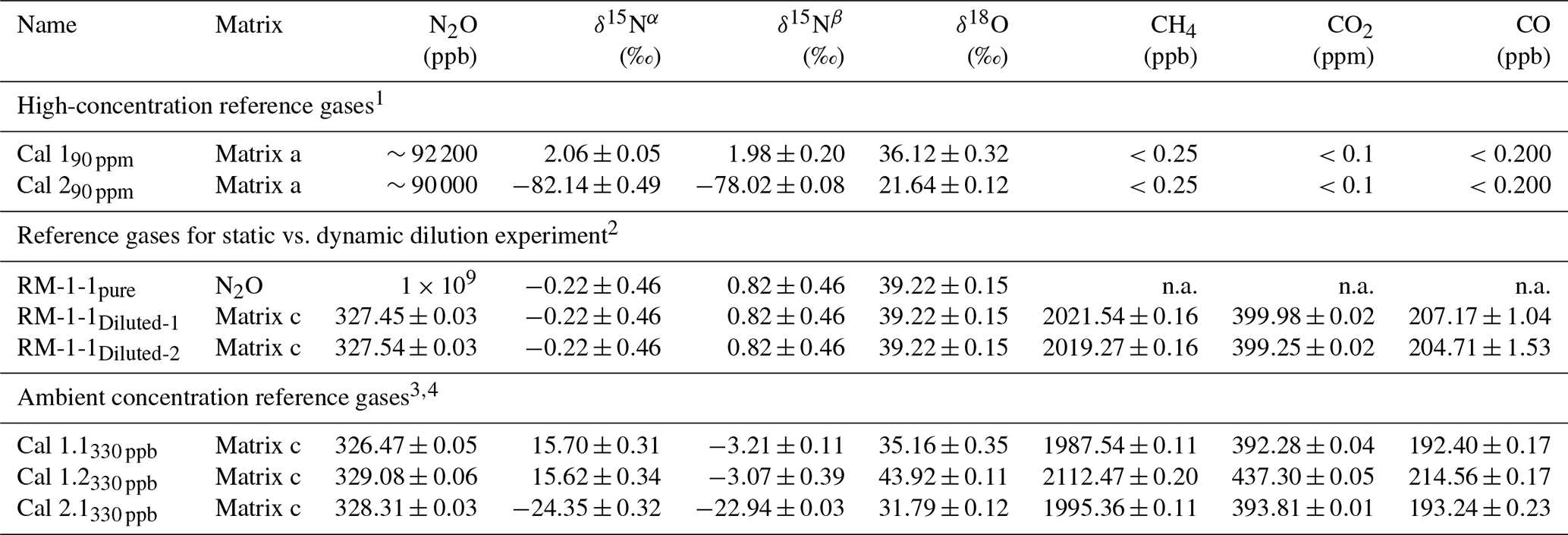
n.a. – not analysed. ¹ N₂O isotopic analysis performed by Sakae Toyoda (Institute of Science Tokyo); indicated uncertainties are standard errors for replicate analysis, but do not enclose the uncertainty of standards applied for calibration. ² N₂O isotopic analysis of RM1-1 pure was performed as described in Mohn et al. (2022). Isotopic composition of diluted standards assumed to be identical to RM1-1_pure, i.e. no isotopic fractionation. N₂O, CH₄, CO₂ and CO concentrations analysed by WCC-Empa against NOAA/ESRL/GMD standards. The indicated uncertainties are standard deviations for replicate analyses. ³ N₂O isotopic analysis of Cal 1.1 and Cal 2.1 performed by Sakae Toyoda (Institute of Science Tokyo); indicated uncertainties are standard errors for replicate analysis but do not enclose uncertainty of standards applied for calibration. Isotopic composition of diluted standards assumed to be identical, i.e. no isotopic fractionation. ⁴ N₂O isotopic analysis of Cal 1.2_330 ppb performed at Empa against primary standards analysed by Science Tokyo; indicated uncertainties are standard deviations for replicate analyses. N₂O, CH₄, CO₂ and CO concentrations analysed by WCC-Empa against NOAA/ESRL/GMD standards. The indicated uncertainties are standard deviations for replicate analyses.

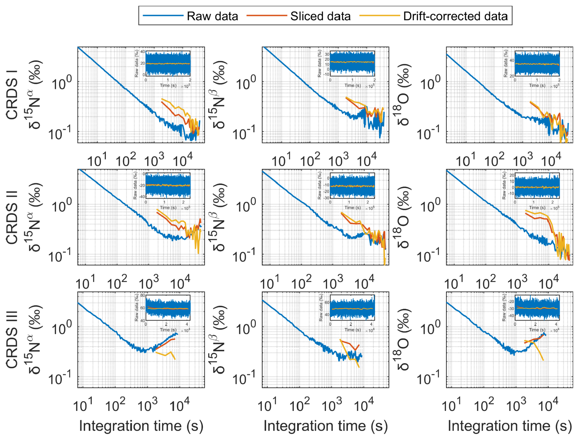
Figure 1 Allan precision for the three tested CRDS analysers (CRDS I, II and III) analysing pressurised air (Cal 1.2_330 ppb; Table 1). Three data sets are presented: Uncorrected raw data recorded at high temporal resolution binned to 15 s time intervals (blue), sliced data averaged at 5 min intervals (red) and drift-corrected 5 min averaged intervals (yellow).

2.2 Spectral simulations

Figure 2 shows a simulated spectrum for typical ambient concentrations of trace gases, i.e. 300 ppb N₂O, 400 ppm CO₂ and 2 ppm CH₄, together with a spectrum measured by the CRDS-I instrument in ambient air, both for the wavenumber window of 2195.7 to 2196.3 cm⁻¹, where the Picarro G5131-i spectrometer operates.

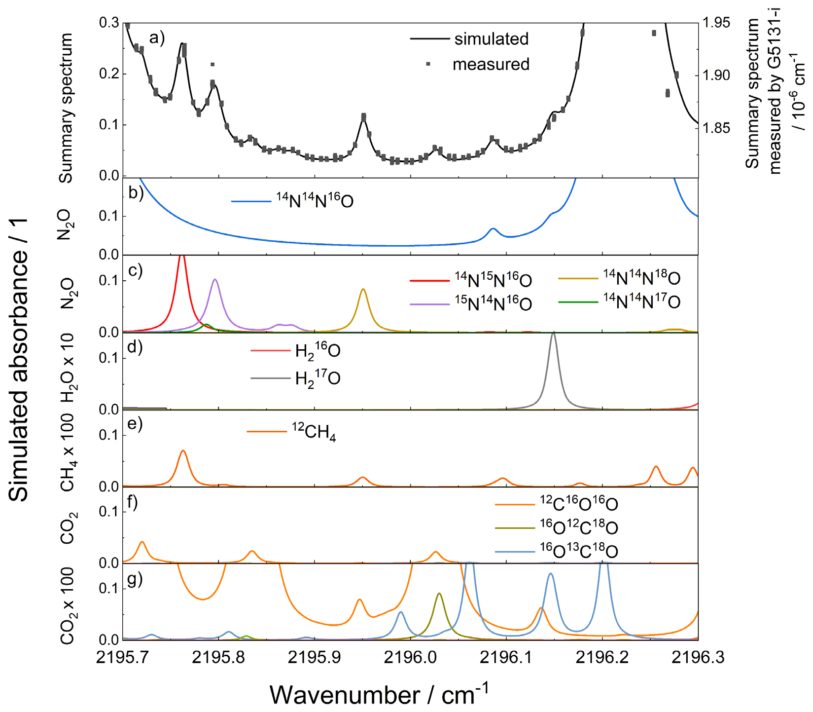
Figure 2 Exemplary spectrum of ambient air measured with a G5131-i analyser (CRDS-I, black squares, right y axis), compared to a simulated spectrum (top graph a, black line, left y axis). The following molecules absorb in the wavelength region and are considered in the simulation: (b) N₂O main isotopologue (¹⁴N¹⁴N¹⁶O, blue line); (c) ¹⁴N¹⁵NO isotopologue (¹⁵N^α, red line), ¹⁵N¹⁴NO (¹⁵N^β, violet line), N₂¹⁸O isotopic species (brown line), ${{\mathrm{N}}_{\mathrm{2}}}^{\mathrm{17}}\mathrm{O}$ isotopic species (green line); (d) H₂O 10× magnification: ${{\mathrm{H}}_{\mathrm{2}}}^{\mathrm{16}}\mathrm{O}$ (black line), ${{\mathrm{H}}_{\mathrm{2}}}^{\mathrm{17}}\mathrm{O}$ (grey line); (e) CH₄ 100× magnification (dark orange line); (f) ¹³CO₂ (orange line); (g) CO₂ 100 magnification: ¹³CO₂ (orange), ¹⁶O¹²C¹⁸O (olive green) and ¹⁶O¹³C¹⁸O (blue). Simulations were performed for 300 ppb N₂O, 400 ppm CO₂, 1 % H₂O and 2 ppm CH₄ in an ambient air matrix at 313 K, 10⁴ Pa and 20 km optical path length.

Spectral simulations were performed using proprietary software written in LabVIEW. The software utilises spectral line data from the HITRAN2020 database (Gordon et al., 2022) to simulate the absorption spectrum, accounting for Doppler broadening of the spectral lines. In addition, pressure broadening by the matrix gas, pressure shift of the spectral lines as well as temperature dependence of the line intensity and line broadening effects were considered. Spectra were simulated for the actual experimental conditions of 313 K gas temperature, 100 hPa gas pressure and 20 km absorption path length. The simulated spectra were fitted using a self-developed algorithm using the Fityk software (Wojdyr, 2010). While the simulations were performed using all spectral lines listed in the HITRAN 2020 database, in the fitting, we only considered those lines that have a measurable contribution to the spectrum within the spectral window of 2195.70–2196.3 cm⁻¹. The fitting approach followed the same principles as described in our recent publication (Pogány et al., 2025). The fitted lines included 19 N₂O lines. Nine lines of the main N₂O isotopic species were fitted as one line set, i.e. the relative line positions as well as ratios of the line intensities were calculated and used as fixed parameters in the fitting, together with Gauss and Lorentz line widths, leaving only the line area and position of the line at 2196.209 cm⁻¹ as free parameters. Three lines of the ¹⁵N^α isotopic species were fitted as a second line set, three lines of both the ¹⁵N^β and the ¹⁴N¹⁴N¹⁷O isotopologue as the third line set, and one ¹⁴N¹⁴N¹⁸O line as a fourth line set. Furthermore, 12 CO₂ lines corresponding to different isotopic species were fitted as a fifth line set. In the line sets numbers 2–5, all line positions are given as fixed parameters relative to the position of the N₂O line at 2196.209 cm⁻¹. The CH₄ lines are so weak compared to the N₂O and CO₂ lines that they cannot be fitted independently; i.e., their influence on the spectrum cannot be considered in the fitting process.

Isotope ratios were calculated from the ratio of the line areas obtained from the spectral fitting, and the line intensities calculated for a temperature of 313 K, according to the following equation:

$$\mathrm{\Delta }\mathit{\delta }=\left[\left({\displaystyle \frac{{\mathit{\alpha }}_{\mathrm{i}}\cdot S_{\mathrm{m}}}{{\mathit{\alpha }}_{\mathrm{m}}\cdot S_{\mathrm{i}}}}\right)-\left({\displaystyle \frac{{\mathit{\alpha }}_{\mathrm{i}}^{\mathrm{330}}\cdot S_{\mathrm{m}}}{{\mathit{\alpha }}_{\mathrm{m}}^{\mathrm{330}}\cdot S_{\mathrm{i}}}}\right)\right]\cdot \mathrm{1000}$$

where α_i is the line area (in cm⁻²) and S_i the line intensity in ${\mathrm{cm}}^{-\mathrm{1}}(\mathrm{molec}.{\mathrm{cm}}^{-\mathrm{2}}{)}^{-\mathrm{1}}$, for the minor, i.e. ¹⁵N^α, ¹⁵N^β or ¹⁴N¹⁶O¹⁸O isotopic species, and a_m the line area and S_m the line intensity for the main N₂O isotopologue. The superscript 330 corresponds to values determined from the spectrum simulated for a gas composition of 330 ppb N₂O in synthetic air containing no CO₂ or CH₄, which we chose as a reference point for the delta values. Relative delta values were calculated as the difference between simulated results for the experimental conditions and reference conditions (330 ppb N₂O in synthetic air), and compared to the experimental results.

2.3 Experimental design, laboratory setup, measurement procedures

2.3.1 Experimental design

In Table 2 the main experiments conducted in this study are given.

Table 2 Overview table of conducted experiments. Matrix b is synthetic air with Ar (N₂ / O₂ / Ar), details on the composition are given in Table 3.

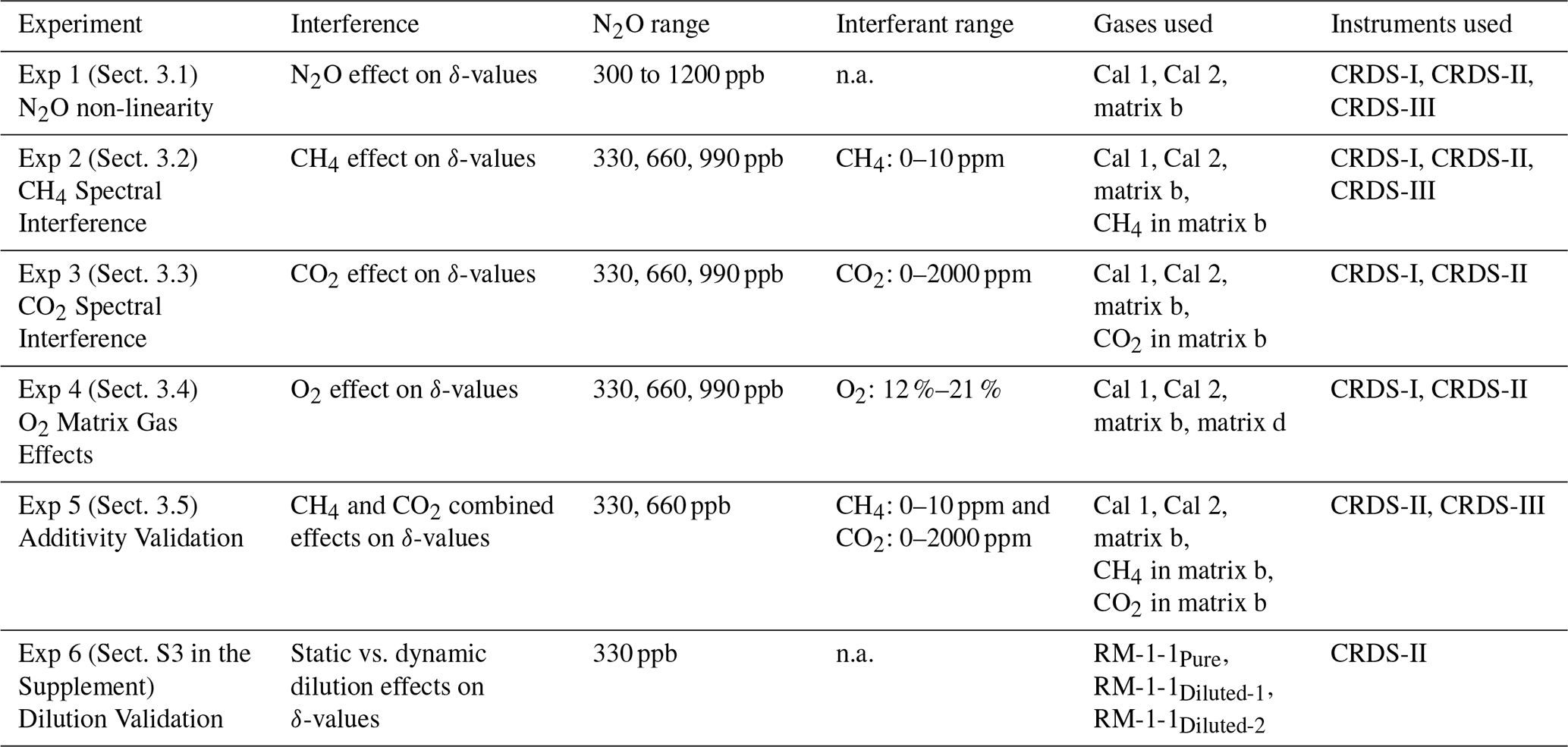
n.a. – not analysed.

2.3.2 Laboratory setup

All experiments were conducted at the Laboratory for Air Pollution / Environmental Technology, Empa, Switzerland, in an air-conditioned laboratory maintained at 295 K (±1 K), with diel variation of ±0.5 K (Saveris 2, Testo AG, Switzerland). Operation in an air-conditioned environment is not a must but supports superior data quality, as shown by Harris et al. (2020). The experiments were conducted using a calibration unit with seven mass flow controllers (MFC) with different flow ranges (2×25, 100, 2×500, 1000, 5000 mL min⁻¹, Vögtlin Instruments GmbH, Switzerland). Availability of MFCs with different flow ranges enabled the simultaneous mixing of N₂O isotope reference gas with a target matrix or spectral interferant and a dilution gas in appropriate proportions to meet the target composition of a sample for a specific experiment. The selection of MFCs was tailored to each experiment in focus, such as investigating N₂O non-linearity, CH₄ and CO₂ spectral interference, gas matrix effects or their combined impact. In a typical experiment, a highly concentrated reference gas (e.g., Cal 1_90 ppm; Cal 2_90 ppm; Table 1) was introduced through a low-flow range MFC channel (25 mL min⁻¹), a matrix or interferant test gas was dosed via a mid-range MFC channel (e.g., 100 mL min⁻¹) and a dilution gas (e.g., matrix b; Table 3) was added by a high-flow range MFC line (e.g., 1000 mL min⁻¹). The gases were combined in desired proportions with the dilution gas serving as a carrier gas to ensure homogenous mixing of the reference and target gases and short response times. This final gas mixture was then routed to the CRDS analysers using PTFE tubing. Additionally, the multi-position valve (MPV) information was electronically integrated into the experimental setup via CRDS-I/II, which controlled the Picarro Valve Sequencer software application. Figure 3 illustrates the general experimental setup, while Sect. S1 in the Supplement provide detailed information on individual experiments.

Table 3 Concentrations of major constituents and trace gases in matrix and interference test gases used in this study.

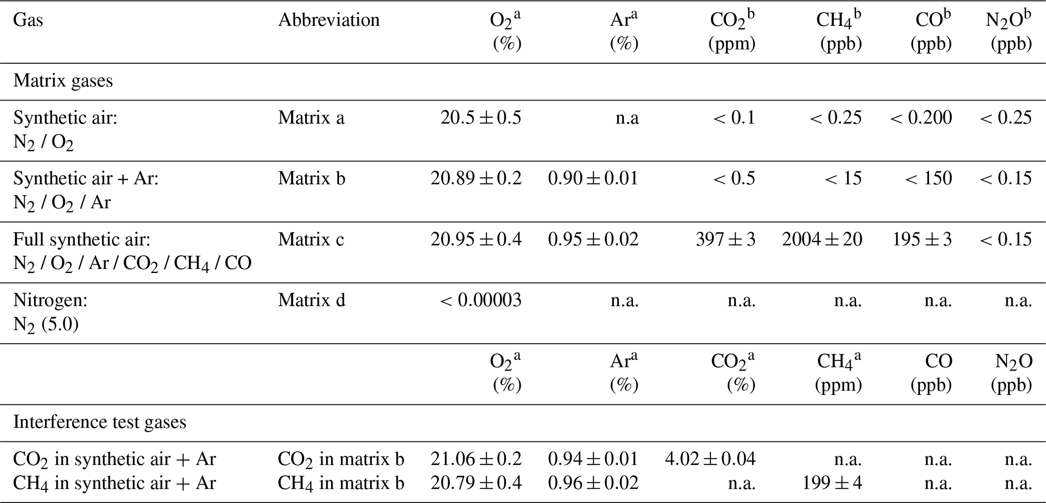
n.a. – not analysed. ^a Manufacturer specifications. ^b Analysed by WCC-Empa against NOAA/ESRL/GMD standards. The indicated uncertainties are standard deviations for replicate analyses.

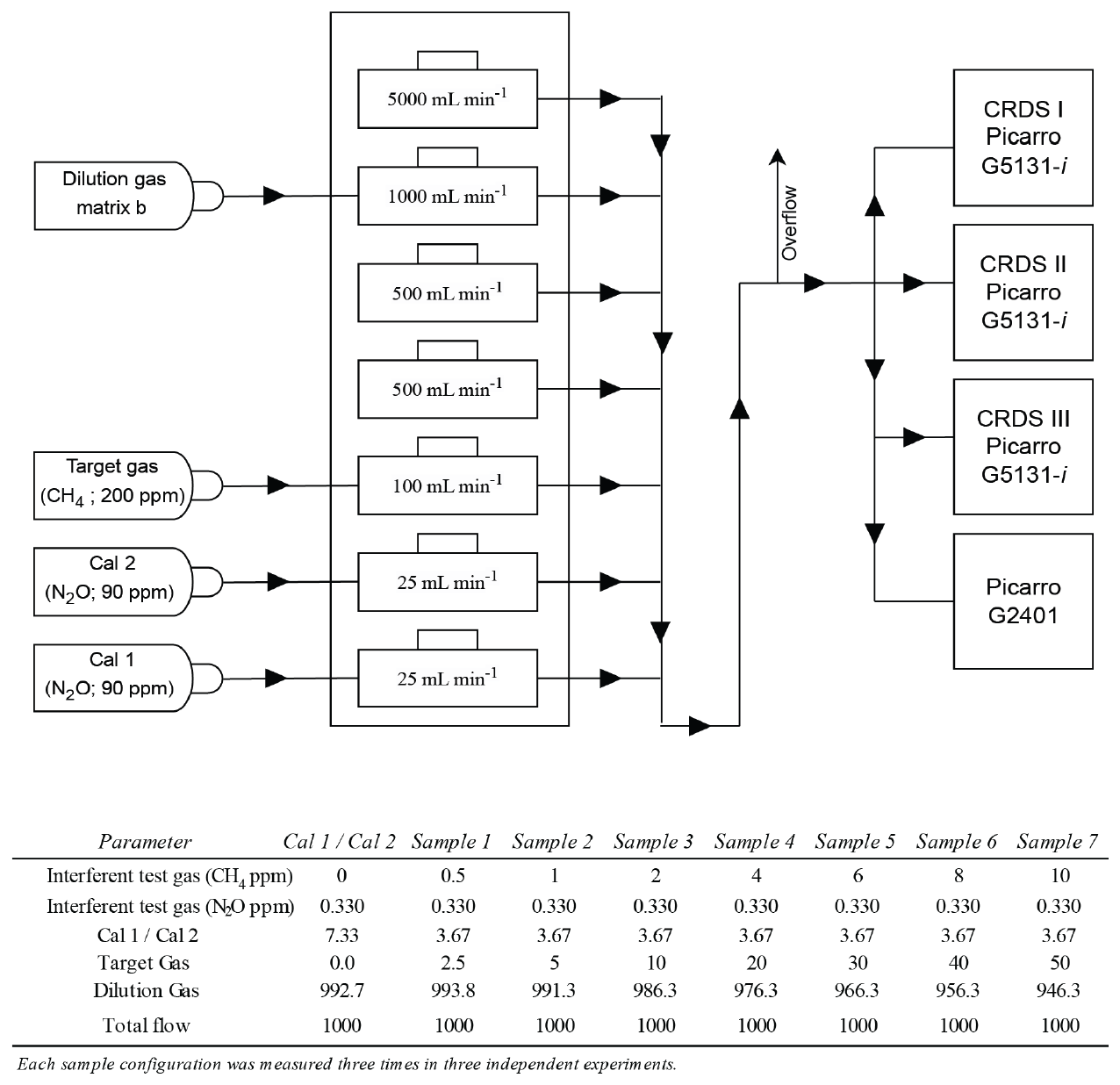
Figure 3 Schematic illustration of the experimental setup used throughout this study in a configuration as applied for an exemplary experiment (Exp. 2, Sect. 3.2). For preparation of gas mixtures, a calibration unit that accommodates seven mass flow controllers (MFCs) was used. The setup allows flexible adjustment of gas flow rates and composition according to the specific requirements of each experiment. In the example shown, the unit was configured to deliver a steady concentration of 330 ppb N₂O at various target concentrations of CH₄ between 0 and 10 ppm (see table above). While apparent N₂O concentrations and isotopic composition were analysed with CRDS-I to -III, the actual interferant (CH₄, CO₂) concentration was determined with a G2401 analyser. Full details on the experimental setups and flow rates, are provided in the Supplement (Sect. S1).

2.3.3 Gas composition of N₂O isotope reference gases and matrix as well as interferant test gases

Table 1 depicts the N₂O mole fraction and associated isotopic compositions of reference gases used in this study. The mole fraction of CH₄, CO₂ and CO in the high-concentration N₂O reference gases were acquired from the specification of their matrix gases, while ambient concentration N₂O reference gases were analysed for their trace gas composition at World Calibration Centre (WCC-Empa, Switzerland) of the World Meteorological Organization (WMO) Global Atmosphere Watch (GAW) program at Empa. WCC-Empa references measurements against reference standards acquired from the National Oceanic and Atmospheric Administration/Earth System Research Laboratory/Global Monitoring Division (NOAA/ESRL/GMD). N₂O isotopic composition is referenced to international isotope ratio scales, Air-N₂ for ${}^{\mathrm{15}}\mathrm{N}{/}^{\mathrm{14}}\mathrm{N}$ and VSMOW for ${}^{\mathrm{18}}\mathrm{O}{/}^{\mathrm{16}}\mathrm{O}$, and $\mathit{\delta }{{}^{\mathrm{15}}\mathrm{N}}^{\text{SP}}$, by analysis of high concentration standards at Institute of Science Tokyo (Cal 1_90 ppm, Cal 2_90 ppm, Cal 1.1, Cal 2.1) or several expert laboratories (RM 1-1 pure) as described in Mohn et al. (2022). For diluted standards (RM 1-1_Diluted-1, RM 1-1_Diluted-2, Cal 1.1_330 ppb, Cal 2.1_330 ppb), we assume identical isotopic composition to high concentration standards, within analytical uncertainties, which was confirmed as described in the Supplement (Sect. S2).

Table 3 outlines the composition of matrix gases and interferant test gases for trace gas concentrations (CH₄, CO₂, CO) and major gas compounds (O₂, Ar, residual N₂). Four different matrix gases were applied: matrix a (synthetic air: N₂ / O₂), matrix b (synthetic air + Ar: N₂ / O₂ / Ar), matrix c (Full synthetic air: N₂ / O₂ / Ar / CO₂ / CH₄ / CO), matrix d (N₂). Matrix gases were analysed at WCC-Empa for the trace gases CO₂, CH₄, H₂O (G1301, Picarro Inc., USA), and N₂O as well as CO (LGR 913-0015-0000; Los Gatos Research Inc., USA). For all matrix gases, the concentration of N₂O was below 0.25 ppb, but accurate detection of N₂O and other trace gas concentrations in the interferant test gases was prevented by spectral interferences of high mole fractions of CO₂ or CH₄ on the respective optical analyser.

2.3.4 Measurements to quantify correction factors and for validation

Experiments for quantifying trace gas interferences, N₂O non-linearity and O₂ matrix gas effects on apparent delta values and validation experiments are summarised in Table 2. The specific target gas concentrations and flows of N₂O reference, matrix or interferant test and dilution gases used for each experiment are detailed in Sect. S1. The experimental workflow consisted of three phases: an initial calibration phase (phase 1), an experimental phase, where apparent effects on delta values were characterised (phase 2), and a final calibration phase (phase 3). During phase 1 and 3, two reference gases (Cal 1_90 ppm and Cal 2_90 ppm; Table 1), with different isotopic compositions, were diluted to ambient N₂O concentrations and measured in triplicate. In phase 2, samples with constant N₂O isotopic composition but differences in gas composition, e.g. concentration of N₂O, CH₄, CO₂, or O₂, were established by dynamic dilution of an N₂O isotope reference gas (Cal 1_90 ppm). Sample analyses were bracketed by measurements of calibration gas 1 (Cal 1_90 ppm) diluted to ambient concentration, but without variation in the interferant, and instrumental drift was corrected using the two nearest Cal 1 measurements. Both sample and reference gases were measured for 15 min per analysis, which was chosen as a compromise between increased precision for longer averaging times and efficiency for gas consumption and workload. The last five minutes of the 15 min sampling period were selected for further data processing. All experiments were conducted in triplicate on at least two or more calendar days. The analyser output data were processed, e.g. drift corrected and calibrated, with the MATLAB code described in Sect. 2.4.

Each data set was fitted using a linear fitting model in MATLAB to obtain the slope and intercept of the fit line. The standard error of the slope was calculated using the following formula:

$$\text{SE}\left(m\right)=\sqrt{{\displaystyle \frac{\mathrm{1}}{n-\mathrm{2}}}\cdot {\displaystyle \frac{\sum (y_{\mathrm{i}}-\widehat{y_{\mathrm{i}}}{)}^{\mathrm{2}}}{\sum (x_{\mathrm{i}}-\stackrel{\mathrm{‾}}{x}{)}^{\mathrm{2}}}}}$$

where; y_i are the actual data points, $\widehat{y_{\mathrm{i}}}$ are the fitted values from the linear model, x_i are the input values, $\stackrel{\mathrm{‾}}{x}$ is the mean of x values, and n is the number of data points. The 95 % confidence bounds are also marked for each fit. The goodness of fit from the model is represented by the adjusted coefficient of determination $R_{\text{adj}}^{\mathrm{2}}$ value which, compared to the R² value also accounts for the number of predictors. The adjusted R² value is given by:

$$R_{\text{adj}}^{\mathrm{2}}=\mathrm{1}-{\displaystyle \frac{(\mathrm{1}-R^{\mathrm{2}})(n-\mathrm{1})}{n-p-\mathrm{1}}}$$

where; n is the number of data points, p is the number of predictors (excluding the intercept), and R² is the coefficient of determination, which is measured as follows:

$$R^{\mathrm{2}}=\mathrm{1}-{\displaystyle \frac{{\text{SS}}_{\text{res}}}{{\text{SS}}_{\text{tot}}}}$$

where; SS_res is the residual sum of squares (sum of squared differences between observed and predicted values), and SS_tot is the total sum of squares (sum of squared differences between observed values and their mean). In this study, values of R²>0.60 (adjusted R²∼0.58 for our dataset) are used as a pragmatic threshold to indicate an adequate representation of the data by a linear model.

2.4 Data processing and MATLAB user application

We developed a customised MATLAB App for correction and calibration of experimental data. While our specific focus was N₂O isotope analysis on ambient air samples with contributions from soil emissions, the approach can be adapted to any application with sequential analysis of gas samples, intermitted by reference gas analyses, such as bag analyses or on-line sampling from a laboratory or field setup.

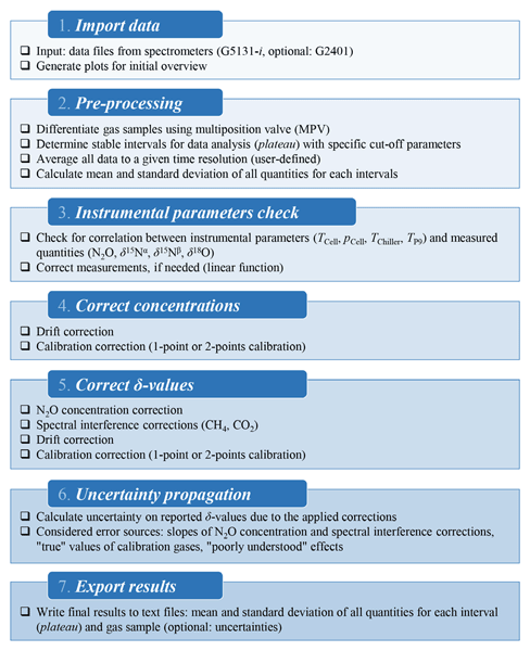
The main functionalities of the code, outlined in Fig. 4, include: data import and pre-processing of N₂O isotope data from a Picarro G5131-i analyser, as well as trace gas concentrations of, CO₂ and CH₄ from a supportive Picarro G2401 analyser, instrumental parameters check, correction and calibration of concentration data, and correction and calibration of δ-values. All corrections are optional and can be individually activated by the user via a graphic user interface. In addition, the code can also provide a propagated uncertainty on the reported δ-values. The approach used for the data treatment, correction and calibration is described below, while a full description of the mathematical model, including all equations, can be found in Appendix A.

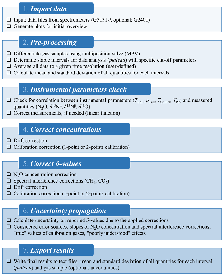
Figure 4 Flowchart illustrating the data post-processing workflow, including data import, plateau identification, co-averaging, parameter-based and drift corrections, calibration, uncertainty assessment and final output. Individual corrections, e.g. for instrument parameters and the uncertainty propagation are optional.

2.4.1 Data import and pre-processing

The output files of the G5131-i analyser, including N₂O concentration and δ-values of the three measured isotopologues ($\mathit{\delta }{{}^{\mathrm{15}}\mathrm{N}}^{\mathit{\alpha }}$, $\mathit{\delta }{{}^{\mathrm{15}}\mathrm{N}}^{\mathit{\beta }}$, δ¹⁸O), and the G2401 analyser, including concentrations of CO, CO₂ and CH₄, are used as input for the MATLAB code. After importing the data, measurement intervals are identified by sample or reference labels and the start/end time for each interval for data analysis (plateau) is defined. For the labelling of measurement intervals, the readout values of the multi-position valve (MPV, EMT-CSD10MWE, Vici AG, Switzerland) of the gas inlet and calibration unit are applied. The readout value of the MPV is used to track gas identity by assigning specific identification numbers to sample and calibration gases useful for post-processing the obtained data (see Sect. 2.3.2). The plateau intervals can be defined by either a fixed duration (e.g., 5 min) before the next switching of the valve position, or by constraining the stability (maximum standard deviation and range) of N₂O concentration and pressure during the interval itself. An option is also provided to import a list of “gas type switch” times and labels from a generic text file, instead of using the output of the MPV (if this is not available). Finally, all data are integrated to a user-defined time resolution (e.g., 15 s), and mean and standard deviation of all quantities are calculated for each interval and gas type at the selected averaging time.

2.4.2 Instrumental parameters check

First, the data are checked for potential correlations of the measured quantities with instrumental parameters of the G5131-i analyser, including cell pressure (p_Cell), cell temperature (T_Cell), chiller temperature (T_Chiller), and P9 (i.e., back-mirror) temperature (T_P9). If a significant correlation is observed between either the N₂O concentration or the δ-values of the different isotopologues ($\mathit{\delta }{{}^{\mathrm{15}}\mathrm{N}}^{\mathit{\alpha }}$, $\mathit{\delta }{{}^{\mathrm{15}}\mathrm{N}}^{\mathit{\beta }}$, δ¹⁸O) and one of the instrumental parameters, the data can be corrected by a linear function (see Appendix A, Eqs. A5 and A6). A “correlation matrix” plot of [N₂O] and all δ-values against all instrumental parameters (showing also R² correlation coefficients) is generated by the code, allowing the user to easily identify anomalous correlations. The slope of the correction function is determined by a linear fit between the raw N₂O concentration (or δ-value) and the considered controlling parameter, recorded during measurements of reference gas 1 (Cal 1). The reason for choosing Cal 1 measurements for this correction was that this gas is measured repetitively over the course of a day. The mean value of the controlling parameter during Cal 1 measurements is used as a reference point, where no correction is applied.

2.4.3 Correction and calibration of N₂O concentration

Before correcting the δ-values, the measured concentrations of N₂O (from G5131-i) and CH₄, CO and CO₂ (from G2401) are corrected for drift and calibrated. The drift correction considers instrumental drifts of measurement signals over time, which manifest by changes in N₂O, CH₄, CO and CO₂ concentrations during Cal 1 measurements. For each sample interval, the “offset” due to drift is calculated as the difference between the linear interpolation of the two nearest (bracketing) Cal 1 intervals and its mean value over all Cal 1 intervals (Eqs. A7 and A8). Consequently, all Cal 1 measurements are corrected to their mean value. Then, the data are calibrated by a one- or two-point calibration correction (Eqs. A9 and A10), depending on the number of available reference gas measurements for which the “true” concentration values are known. For a single calibration gas (Cal 1), this corresponds to the offset of all data by the difference between the mean of all Cal 1 measurements and its “true” value.

2.4.4 Correction and calibration of δ-values

The correction and calibration of the δ-values consists of four steps: N₂O concentration correction, CH₄ and CO₂ spectral interference corrections, drift correction and calibration correction.

The N₂O concentration correction considers the apparent dependencies of the isotopic readings ($\mathit{\delta }{{}^{\mathrm{15}}\mathrm{N}}^{\mathit{\alpha }}$, $\mathit{\delta }{{}^{\mathrm{15}}\mathrm{N}}^{\mathit{\beta }}$, δ¹⁸O) of the analyser on the N₂O concentration. Based on observations from three analysers, the N₂O concentration dependency is assumed to be proportional to the inverse of the N₂O concentration (i.e., $\mathrm{1}/\left[{\mathrm{N}}_{\mathrm{2}}\mathrm{O}\right]$) (see Appendix A, Eq. A12). Importantly, the slope of the correction line (to be defined by the user) is analyser-specific and must be experimentally quantified for any specific analyser by means of a dedicated experiment with varying N₂O concentration at constant isotopic composition (as done in this work). The mean N₂O concentration of Cal 1 is used as a reference point, where no correction is applied.

The spectral interference corrections (for CH₄, CO₂) consider spectral interference effects by neighbouring CH₄ and CO₂ absorption lines on the $\mathit{\delta }{{}^{\mathrm{15}}\mathrm{N}}^{\mathit{\alpha }}$, $\mathit{\delta }{{}^{\mathrm{15}}\mathrm{N}}^{\mathit{\beta }}$, and δ¹⁸O retrievals of G5131-i. These effects have been shown to be proportional to the $\left[{\mathrm{CH}}_{\mathrm{4}}\right]/\left[{\mathrm{N}}_{\mathrm{2}}\mathrm{O}\right]$ and $\left[{\mathrm{CO}}_{\mathrm{2}}\right]/\left[{\mathrm{N}}_{\mathrm{2}}\mathrm{O}\right]$ ratios, respectively (Harris et al., 2020) (Appendix A, Eqs. A13–A14). Again, the slope of the correction line is user-defined and must be experimentally quantified by means of dedicated experiments with varying CH₄ and CO₂ concentrations at constant isotopic composition. The mean CH₄ and CO₂ concentrations of Cal 1 are used as reference points, where no correction is applied.

Then, a drift correction is applied to all δ-values, calculated as for the concentration corrections (see Eq. A15), and finally the δ-values are calibrated by a one- or two-point calibration correction (Eqs. A16 and A17). The calibration function is calculated based on the measured and the “true” values of $\mathit{\delta }{{}^{\mathrm{15}}\mathrm{N}}^{\mathit{\alpha }}$, $\mathit{\delta }{{}^{\mathrm{15}}\mathrm{N}}^{\mathit{\beta }}$, and δ¹⁸O of Cal 1 (1-point calibration, i.e. offset), or both Cal 1 and reference gas 2 (Cal 2), if available (2-point calibration).

2.4.5 Uncertainty propagation and data export

The established MATLAB code has the potential to optionally calculate a propagated uncertainty for the reported δ-values. For this, the law of error propagation (JCGM, 2008), exemplified for CH₄ isotopic species in Sperlich et al. (2024) was applied to the mathematical framework used to calculate the δ-values. The considered error sources include uncertainties in the slopes applied for the N₂O concentration correction, the spectral interference corrections, uncertainties in the δ-values attributed to reference gases, and uncertainties due to poorly understood effects, which were approximated by repeatability for target gas measurements. The equations used for error propagation, including individual derivatives of the measurement model for each error term, are presented in Appendix A (Eqs. A18–A28). While the functionality of the uncertainty propagation was implemented in the MATLAB algorithm for future use, it was not tested in this study.

After all corrections have been applied, the results can be exported as ASCII (text) files, including the mean and standard deviation of all quantities for each measurement interval (plateau) and sample gas, plus optionally, the propagated uncertainty, comprising all relevant contributions. In addition, a “logfile” text file is generated, documenting information on every applied correction and its corresponding input parameters.

3 Results

In the following sections, the apparent δ-values of N₂O for the tested G5131-i analysers under changing N₂O, CH₄, CO₂ and O₂ concentrations (Sect. 3.1–3.4) are provided. The determined regression slopes or interference coefficients, $m_{{\mathrm{N}}_{\mathrm{2}}\mathrm{O}}$, $m_{{\mathrm{CO}}_{\mathrm{2}}}$, $m_{{\mathrm{CH}}_{\mathrm{4}}}$ and $m_{{\mathrm{O}}_{\mathrm{2}}}$, for all experiments are given in Tables 4–7 and are used to parametrise the MATLAB algorithm. To confirm mathematical corrections and provide insights into spectral analysis and data post-processing of the analysers, the simulated interference coefficients are given for comparison. In a next step, the additivity of N₂O, CH₄ and CO₂ concentration effects is tested in a validation study (Sect. 3.5).

3.1 N₂O non-linearity (Exp. 1)

Although the three tested CRDS analysers are the same analyser model, they offer different N₂O operation ranges, i.e. CRDS-II and -III displayed increasing data loss already above ∼700–800 ppb N₂O, which most probably is related to enhanced absorption of the empty cavity (e.g. by dust particles) and therefore partial saturation of the absorption features at higher N₂O concentrations. Therefore, only CRDS-I was tested in between 330 and 1200 ppb N₂O, while CRDS-II and -III were only operated up to 800 ppb N₂O. Figure 5 provides dependencies of apparent δ-values of N₂O isotopologues ($\mathrm{\Delta }\mathit{\delta }{{}^{\mathrm{15}}\mathrm{N}}^{\mathit{\alpha }}$, $\mathrm{\Delta }\mathit{\delta }{{}^{\mathrm{15}}\mathrm{N}}^{\mathit{\beta }}$, Δδ¹⁸O) on inverse N₂O concentrations for all three G5131-i analysers as well as for simulated results. The experimentally determined regression slopes $m_{{\mathrm{N}}_{\mathrm{2}}\mathrm{O}}$ are applied to parametrise the developed MATLAB algorithm. Consistency of apparent δ-values from triplicate analyses for individual analysers confirms reproducible offsets, within short timeframes, between measured and true δ-values for N₂O concentration changes between sample and calibration gases (Fig. 5). A linear relationship between apparent delta values and the inverse N₂O concentration has already been observed by Harris et al. (2020). A closer look at the results of spectral simulations displays a slightly non-linear behaviour of the apparent isotope effect. For the experimental data, this effect is masked by instrumental precision, and therefore a linear correction was applied.

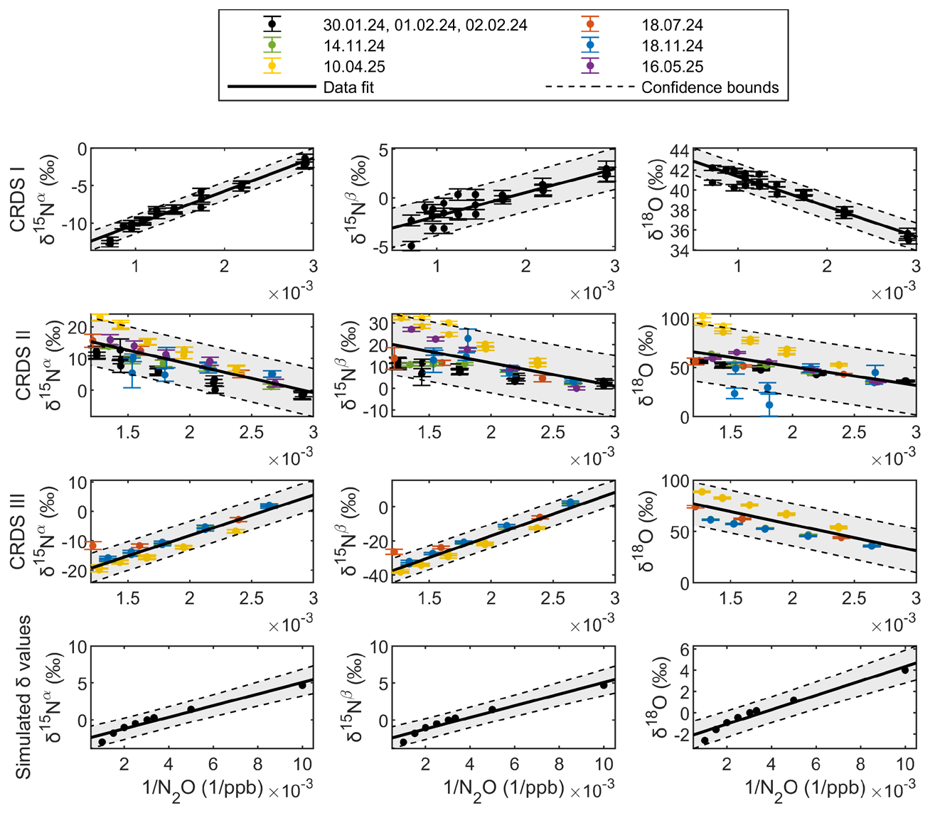
Figure 5 Apparent changes in N₂O isotopic composition versus $\mathrm{1}/{\mathrm{N}}_{\mathrm{2}}\mathrm{O}$. In the top three rows, experimental data for three CRDS analysers (CRDS I, CRDS II and CRDS III) are provided. The coloured points represent the data sets measured on different days. For CRDS I, the data points are combined into a single cluster (black symbols), since they were measured over only four days. Each data point presents an average of 5 min of sample measurement. The error bars represent the standard errors, calculated by incorporating the standard deviations from both the sample measurements and the neighbouring calibration gas measurements. The regression line is plotted in black (slope is $m_{{\mathrm{N}}_{\mathrm{2}}\mathrm{O}}$), corresponding to the combined coefficient in Table 4, while the black shaded area shows the 95 % confidence bounds of this fit. The bottom row shows the simulated difference in delta values to 330 ppb plotted as a function of $\mathrm{1}/{\mathrm{N}}_{\mathrm{2}}\mathrm{O}$. The slope, intercept and adjusted R² values for each data set are presented in Table 4.

Clearly, the different analyser specimens (CRDS-I, CRDS-II, CRDS-III) and simulated results show contrasting regression slopes ($m_{{\mathrm{N}}_{\mathrm{2}}\mathrm{O}}$) (Table 4). Repetitive tests of individual analysers over longer timescales, such as several weeks or months, indicate that the N₂O non-linearity correction is not only analyser-specific but also variable over time. CRDS-III tested here was already included in an earlier study (CRDS II in Harris et al., 2020), but with substantially different non-linearity behaviour. Similarly, dependencies of delta values on N₂O concentration changed significantly for CRDS-II, which was tested several times. The situation is complicated by the fact that the analyser software has a built-in post-correction to minimise N₂O non-linearities, which is parametrised analyser-specific by Picarro Inc.

Table 4 Experimentally derived correction functions for N₂O non-linearity of CRDS analysers and spectral simulations. The correction slope $m_{{\mathrm{N}}_{\mathrm{2}}\mathrm{O}}$ is given in ‰ ppb, the intercept in ‰.

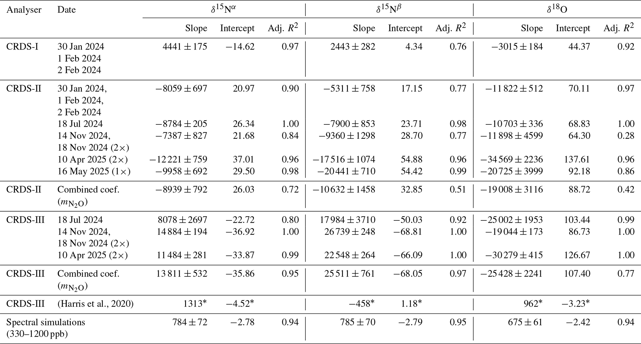
^* Correction slopes as given in Fig. S4-3 of Harris et al. (2020).

3.2 CH₄ spectral interference (Exp. 2)

Figure 6 shows the effect of CH₄ concentration changes, between 0 and 10 ppm, on apparent N₂O delta values ($\mathrm{\Delta }\mathit{\delta }{{}^{\mathrm{15}}\mathrm{N}}^{\mathit{\alpha }}$, $\mathrm{\Delta }\mathit{\delta }{{}^{\mathrm{15}}\mathrm{N}}^{\mathit{\beta }}$, Δδ¹⁸O) for three different N₂O concentrations (330, 660 and 990 ppb). Delta values display a linear relationship on ${\mathrm{CH}}_{\mathrm{4}}/{\mathrm{N}}_{\mathrm{2}}\mathrm{O}$ concentration ratios, i.e., the interference effect doubles for samples with either a twofold CH₄ concentration or halving the N₂O concentration. Dependencies of apparent delta values on CH₄ concentrations are most substantial for $\mathit{\delta }{{}^{\mathrm{15}}\mathrm{N}}^{\mathit{\alpha }}$, intermediate for δ¹⁸O and weakest for $\mathit{\delta }{{}^{\mathrm{15}}\mathrm{N}}^{\mathit{\beta }}$ (Table 5). Results are generally consistent for repeated experiments (n=3) and between analyser specimens (CRDS I, CRDS II, CRDS-III) as well as with literature data (Harris et al., 2020), which indicates that corrections might be specific for this particular CRDS analyser model (G5131-i) and constant over time. For analysers CRDS-II and CRDS-III, the upper N₂O concentration limit for obtaining precise measurement data is 800 ppb due to enhanced background signals (see Sect. 3.1); therefore, experimental data obtained at 990 ppb were excluded from data analysis. Our spectral simulations underpin the experimental results, although correction slopes for $\mathit{\delta }{{}^{\mathrm{15}}\mathrm{N}}^{\mathit{\alpha }}$ are significantly smaller compared to experimental results (Table 5).

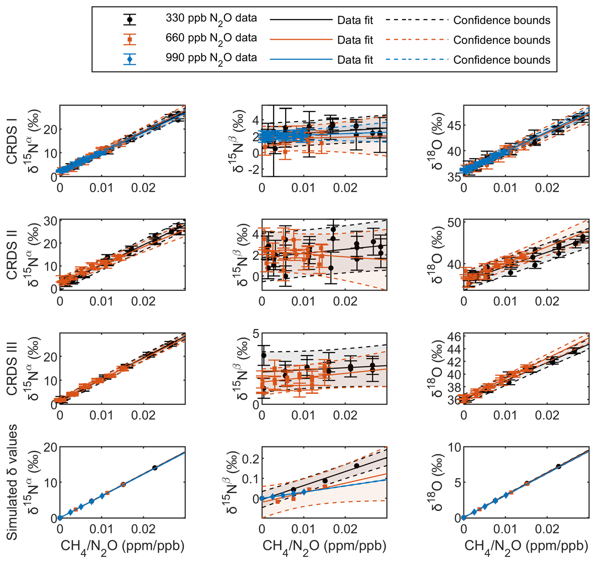
Figure 6 Apparent changes in N₂O isotopic composition versus ${\mathrm{CH}}_{\mathrm{4}}/{\mathrm{N}}_{\mathrm{2}}\mathrm{O}$ for three CRDS analysers (top three rows CRDS-I, II and III) as well as spectral simulations (bottom row). The experimental data points for varying CH₄ concentration but at a constant N₂O concentration are shown with different colour coding, black (330 ppb), orange (660 ppb) and blue (990 ppb), respectively. Each data point corresponds to the mean of three replicate measurements, where each replicate represents an average over 5 min. The error bars represent the standard errors, calculated by incorporating the standard deviations from both the sample measurements and the neighbouring calibration gas measurements. The regression lines for individual N₂O concentrations are plotted in black (330 ppb), orange (660 ppb) and blue (990 ppb), while shaded areas show the 95 % confidence bounds of the corresponding fits. The bottom row shows the simulated difference in delta values to 330 ppb plotted as a function of ${\mathrm{CH}}_{\mathrm{4}}/{\mathrm{N}}_{\mathrm{2}}\mathrm{O}$ The slope, intercept and adjusted R² values for each data set are presented in Table 5.

Table 5 Experimentally derived correction functions for CH₄ spectral interference of CRDS analysers and simulated results. The correction slope $m_{{\mathrm{NCH}}_{\mathrm{4}}}$ is given in ‰ [ppb N₂O] [ppm CH₄]⁻¹, the intercept in ‰.

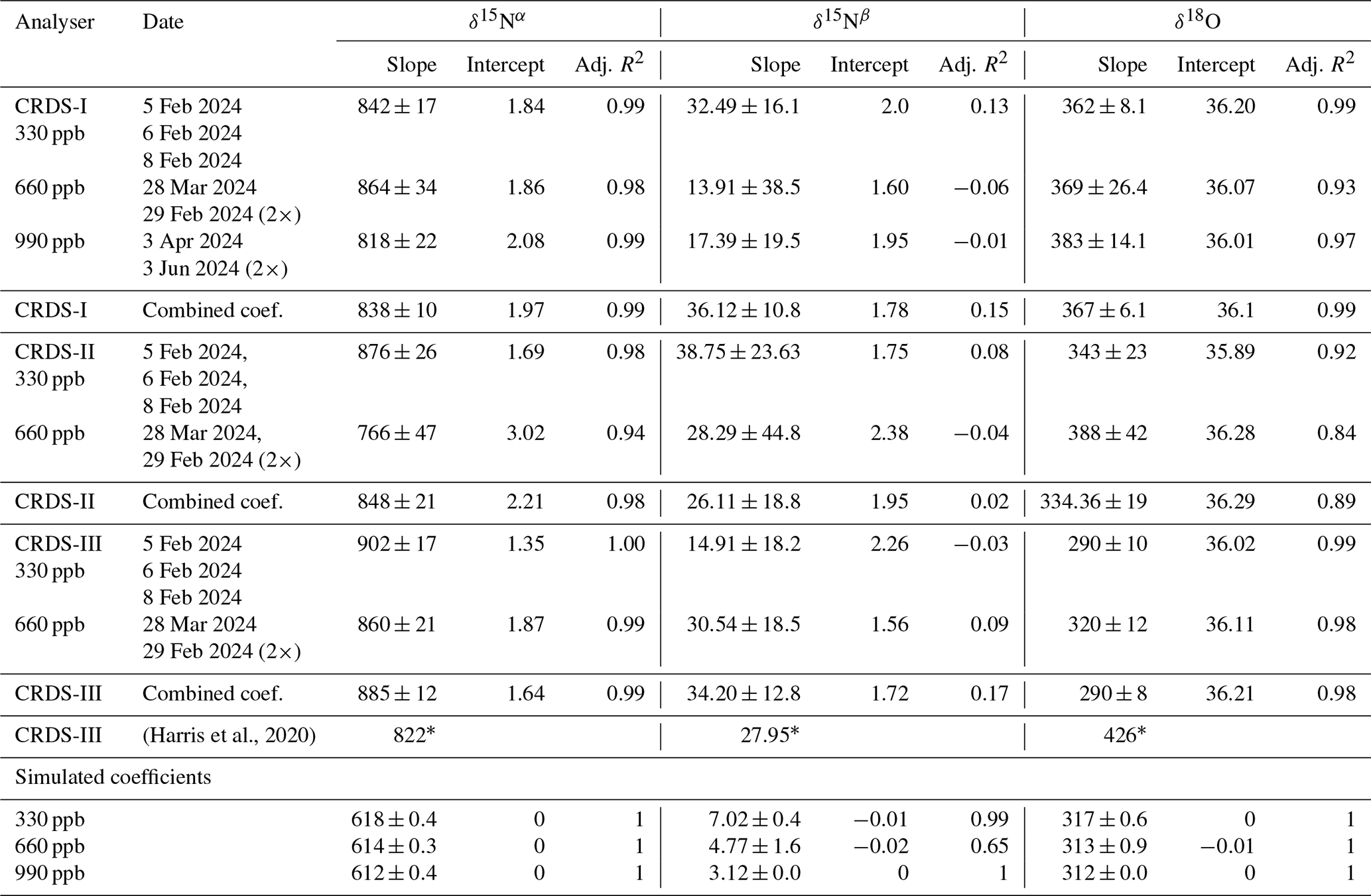
^* Correction slopes as given in Fig. S4-7 of Harris et al. (2020) for 330 ppb N₂O.

The strong spectral interference, observed for $\mathit{\delta }{{}^{\mathrm{15}}\mathrm{N}}^{\mathit{\alpha }}$, can be explained by two CH₄ spectral lines at 2195.762 cm⁻¹ and 2195.764 cm⁻¹, with line intensities of $\mathrm{1.02}\times {\mathrm{10}}^{-\mathrm{24}}$ cm⁻¹ and $\mathrm{4.49}\times {\mathrm{10}}^{-\mathrm{25}}$ cm⁻¹, respectively (see Fig. 2). The spectral interference on δ¹⁸O is a factor of two (for simulations) to three (for experimental results) weaker and caused by a single CH₄ line at 2195.95 cm⁻¹ with a line intensity of $\mathrm{4.26}\times {\mathrm{10}}^{-\mathrm{25}}$ cm⁻¹, overlapping with the N₂¹⁸O line. In the case of the ¹⁵N^β isotopologue, the overlapping CH₄ line is approximately an order of magnitude weaker with a line intensity of $\mathrm{5.148}\times {\mathrm{10}}^{-\mathrm{26}}$ cm⁻¹; thus, the observed spectral interference and its effect on the δ-values are negligible. The main analytical challenge with respect to the CH₄ interference is the fact, that all CH₄ lines co-evolve with N₂O lines, so no specific CH₄ concentration analysis is feasible within the wavelength region implemented in the G5131-i analyser. Therefore, the most straightforward approach is an empirical post-correction using an independent CH₄ concentration analyser, as suggested and implemented in this manuscript.

3.3 CO₂ spectral interference (Exp. 3)

Figure 7 displays the effect of CO₂ concentration changes in the range 0 to 2000 ppm on apparent δ-values for experimental results (CRDS-I and II) and spectral simulations. Experiments were conducted for three different N₂O concentrations, 330, 660 and 990 ppb, with each experiment repeated three times. CRDS-II was not capable to analyse gas mixtures at 990 ppb due to enhanced background and saturation effects (see Sect. 3.1). Overall, no consistent and significant effect of ${\mathrm{CO}}_{\mathrm{2}}/{\mathrm{N}}_{\mathrm{2}}\mathrm{O}$ concentration changes on apparent δ-values was observed for the two analyser specimens (Fig. 7; Table 6). These results are in agreement with observations made by Harris et al. (2020) and imply that the interfering CO₂ absorption lines are either well enough separated or the CRDS quantification algorithm is able to correct effects appropriately. In contrast, spectral simulations indicate a stronger, significant spectral interference of CO₂ concentrations on the apparent isotopic delta values for $\mathit{\delta }{{}^{\mathrm{15}}\mathrm{N}}^{\mathit{\beta }}$ and δ¹⁸O, and a minor effect on $\mathit{\delta }{{}^{\mathrm{15}}\mathrm{N}}^{\mathit{\alpha }}$. Apparent effects of up to 8 ‰ for $\mathit{\delta }{{}^{\mathrm{15}}\mathrm{N}}^{\mathit{\beta }}$ and δ¹⁸O values are most probably due to computational differences between the spectral simulation and the analyser's fitting software.

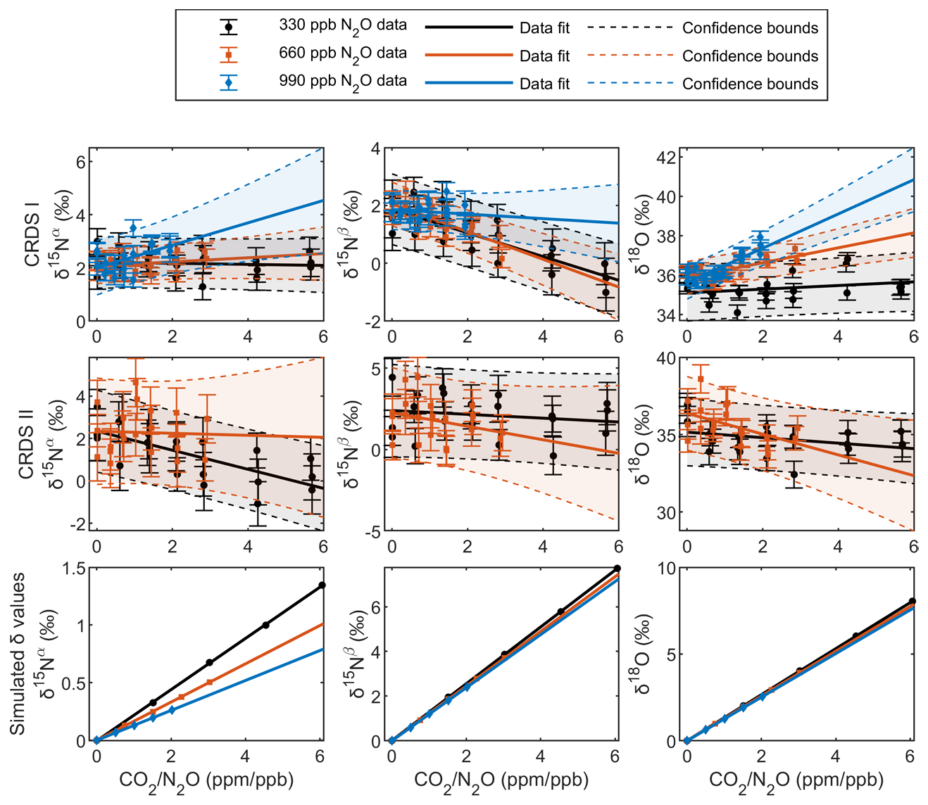
Figure 7 Apparent changes in N₂O isotopic composition versus ${\mathrm{CO}}_{\mathrm{2}}/{\mathrm{N}}_{\mathrm{2}}\mathrm{O}$ for two CRDS analysers (top two rows, CRDS-I and II) as well as spectral simulations (bottom row). The experimental data points for varying CO₂ concentration but at a constant N₂O concentration are shown with different colour coding, black (330 ppb), orange (660 ppb) and blue (990 ppb), respectively. Each data point corresponds to the mean of three replicate measurements, where each replicate represents an average over 5 min. The error bars represent the standard errors, calculated by incorporating the standard deviations from both the sample measurements and the neighbouring calibration gas measurements. The regression lines for individual N₂O concentrations are plotted in black (330 ppb), orange (660 ppb) and blue (990 ppb), while shaded areas show the 95 % confidence bounds of the corresponding fits. The bottom row shows the simulated difference in delta values to 330 ppb plotted as a function of ${\mathrm{CO}}_{\mathrm{2}}/{\mathrm{N}}_{\mathrm{2}}\mathrm{O}$. The slope, intercept and adjusted R² values for each data set are presented in Table 6.

Table 6 Experimentally derived correction functions for CO₂ spectral interference of CRDS analysers and simulated results. The correction slope $m_{{\mathrm{CO}}_{\mathrm{2}}}$ is given in ‰ [ppb N₂O] [ppm CO₂]⁻¹, the intercept in ‰.

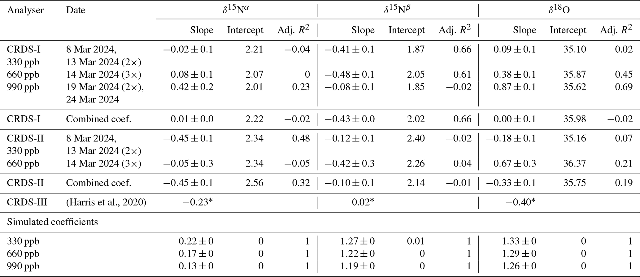
^* Correction slopes as given in Fig. S4-6 of Harris et al. (2020) for 330 ppb N₂O.

3.4 O₂ matrix gas effects (Exp. 4)

Figure 8 shows the effect of O₂ concentration changes in the range 12 % to 21 % on apparent δ-values. Experiments were repeated thrice for a constant N₂O concentration of 330, 660 and 990 ppb (CRDS-I) or 330 and 660 ppb (CRDS-II). The experimental data fits well to a linear model, and the regression coefficients, their corresponding uncertainties and the adjusted R² values are provided in Table 7. The coefficient values are in agreement for the two analyser specimens, for different N₂O concentrations and also with results from Harris et al. (2020). Based on the results, it can be inferred that an instrument-specific correction is applicable for O₂ effects on apparent delta values. However, corrections for $\mathrm{\Delta }\mathit{\delta }{{}^{\mathrm{15}}\mathrm{N}}^{\mathit{\beta }}$ andΔδ¹⁸O at 330 ppb N₂O should be applied with caution, as our experimental data indicate low adjusted R² values for both CRDS-I and CRDS-II (Fig. 8). A correction term for the O₂ matrix gas effect was not included in the MATLAB code, as no relevant oxygen concentration changes are expected for the target application, N₂O emissions from soils.

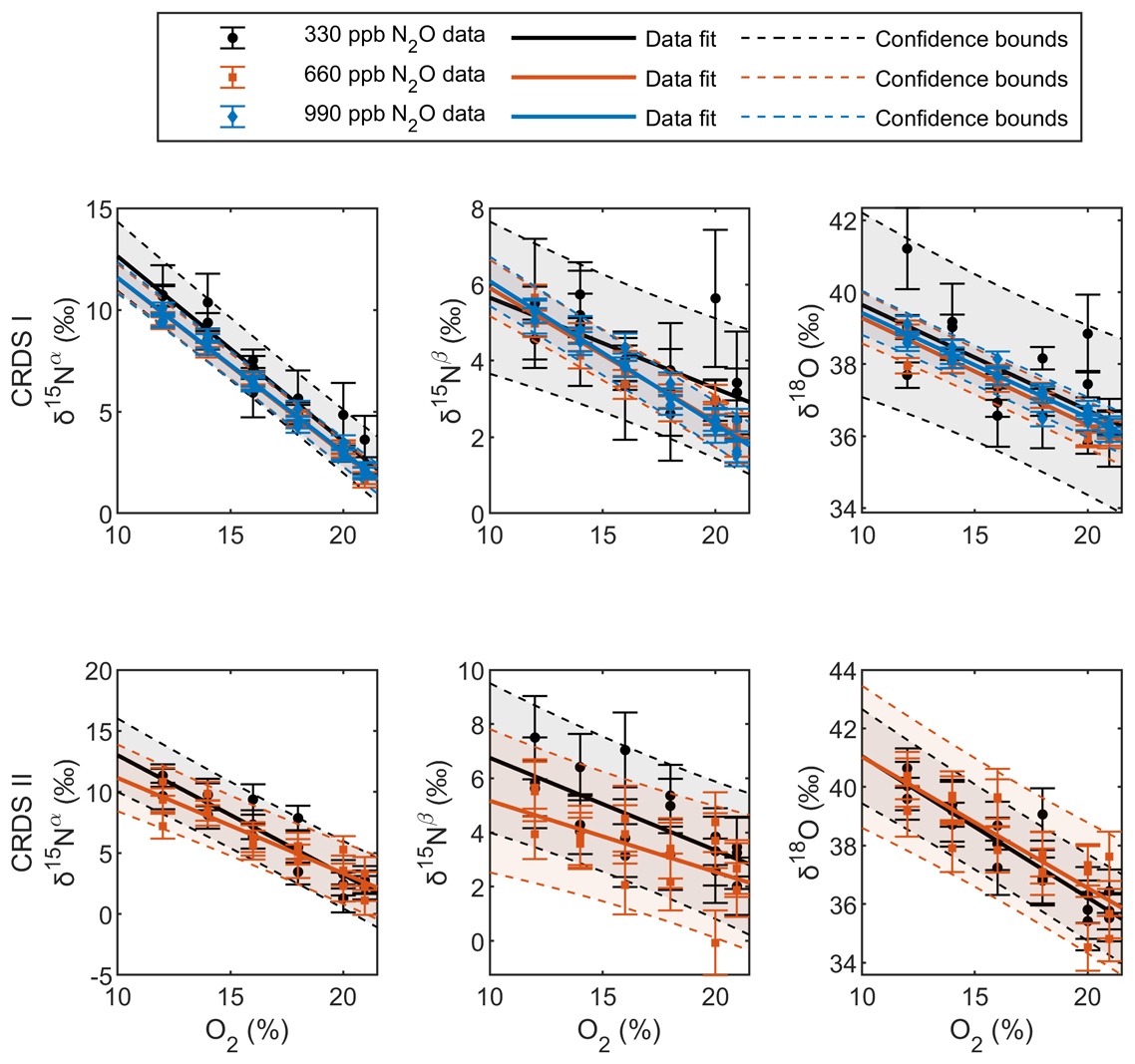
Figure 8 Apparent changes in N₂O isotopic composition versus O₂ concentration change for two CRDS analysers (CRDS I and II). The experimental data points for varying O₂ concentration but at a constant N₂O concentration are shown with different colour coding, black (330 ppb), orange (660 ppb) and blue (990 ppb). Each data point corresponds to the mean of three replicate measurements, where each replicate represents an average over 5 min. The error bars represent the standard errors, calculated by incorporating the standard deviations from both the sample measurements and the neighbouring calibration gas measurements. The regression line for each N₂O concentration is plotted in black (330 ppb), orange (660 ppb) and blue (990 ppb), while shaded areas show the 95 % confidence bounds of the corresponding fits. The slope, intercept and adjusted R² values for each data set are presented in Table 7.

Table 7 Experimentally derived correction functions for O₂ matrix gas effect of CRDS analysers and simulated results. The correction slope $m_{{\mathrm{O}}_{\mathrm{2}}}$ is given in ‰ [% O₂]⁻¹, the intercept in ‰.

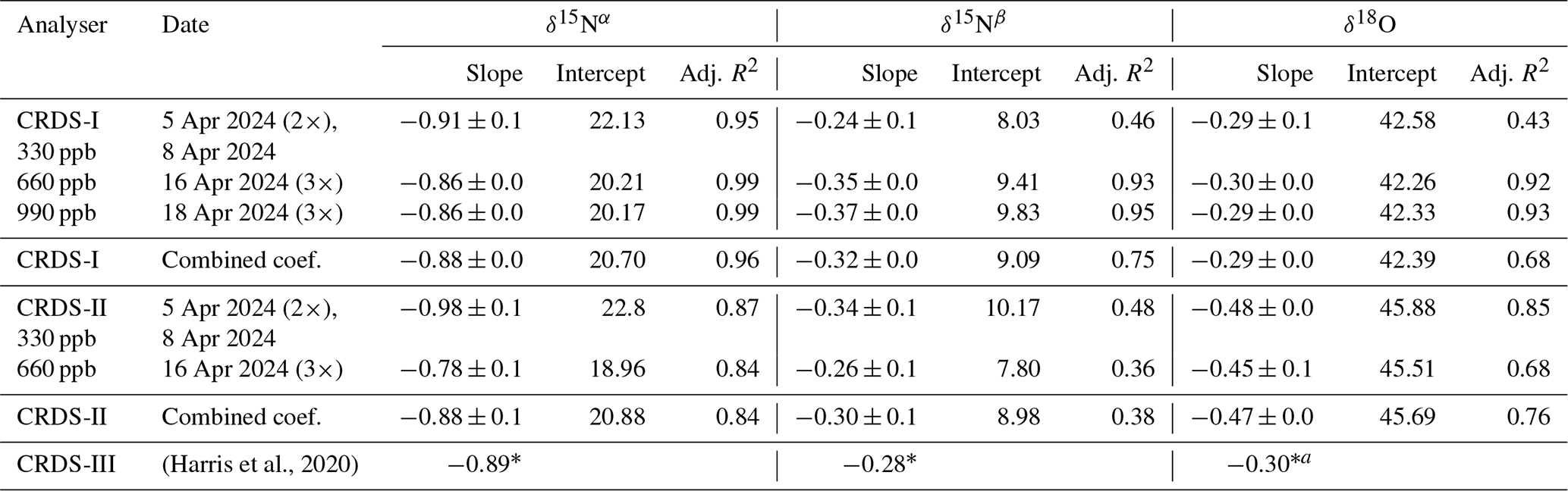
^* Correction slopes as given in Fig. S4-4 of Harris et al. (2020) for 330 ppb N₂O.

3.5 Validation experiments to test combined effects of N₂O, CH₄ and CO₂ concentration changes (Exp. 5)

Experiments involving the simultaneous addition of two interfering gases (CH₄ and CO₂) at two different N₂O concentrations (330 ppb (Exp. 5a) and 660 ppb (Exp. 5b)) were conducted to assess the practicality of the developed MATLAB code and test whether the established correction functions are additive or require a more complex correction algorithm. Apparent delta values were corrected for CH₄ and CO₂ spectral interference as well as N₂O non-linearity using the mathematical formalism described in Appendix A and analyser specific average, i.e. combined, corrections factors given in Tables 4–6. For CO₂ interference correction of CRDS-III, correction factors of CRDS-II were applied, which was justified by consistent results for two analyser specimen (CRDS-I and II). Figures 9 and 10 illustrate the combined effects of simultaneously increasing CH₄ (0–10 ppm) and CO₂ (0–2000 ppm) concentrations on apparent δ-values at two different N₂O concentrations (330 ppb, Fig. 9, 660 ppb, Fig. 10) for the two tested analysers (CRDS-II and III). CH₄ and CO₂ concentrations were increased stepwise from 0 to 10 ppm (2.5 ppm per step) and 0 to 2000 ppm (500 ppm per step), respectively (see Tables S11 and S12 in the Supplement for further details). Our basic assumption was that spectral interferences by the combined addition of CH₄ and CO₂ for $\mathit{\delta }{{}^{\mathrm{15}}\mathrm{N}}^{\mathit{\alpha }}$ and δ¹⁸O are predominantly driven by CH₄, while interference effects of CH₄ and CO₂ on $\mathit{\delta }{{}^{\mathrm{15}}\mathrm{N}}^{\mathit{\beta }}$ are more balanced. However, the apparent effects on δ-values resulting from simultaneous CH₄ and CO₂ addition (Fig. 9, black squares) deviate significantly from the predetermined correction function for CH₄-only addition (Fig. 6; Table 5). As a result, the fully corrected delta values (black squares) deviate from actual δ-values for all isotopologues. It is also noteworthy that the correction function for ${\mathrm{CH}}_{\mathrm{4}}/{\mathrm{N}}_{\mathrm{2}}\mathrm{O}$ is well-defined with respect to $\mathit{\delta }{{}^{\mathrm{15}}\mathrm{N}}^{\mathit{\alpha }}$ and δ¹⁸O but less substantial for $\mathit{\delta }{{}^{\mathrm{15}}\mathrm{N}}^{\mathit{\beta }}$ (Fig. 6). However, in the validation experiment with simultaneous increases of CH₄ and CO₂ concentrations, the spectral interference on apparent $\mathit{\delta }{{}^{\mathrm{15}}\mathrm{N}}^{\mathit{\beta }}$ values is substantial (Fig. 9). Another notable observation in this validation experiment is that the observed non-corrected data for $\mathit{\delta }{{}^{\mathrm{15}}\mathrm{N}}^{\mathit{\alpha }}$ agrees substantially better with ${\mathrm{CH}}_{\mathrm{4}}/{\mathrm{N}}_{\mathrm{2}}\mathrm{O}$ correction function derived from spectral simulation than with the one obtained in experiment 2 (CH₄ addition without CO₂) (not shown). The reasoning for this connection, however, is unclear.

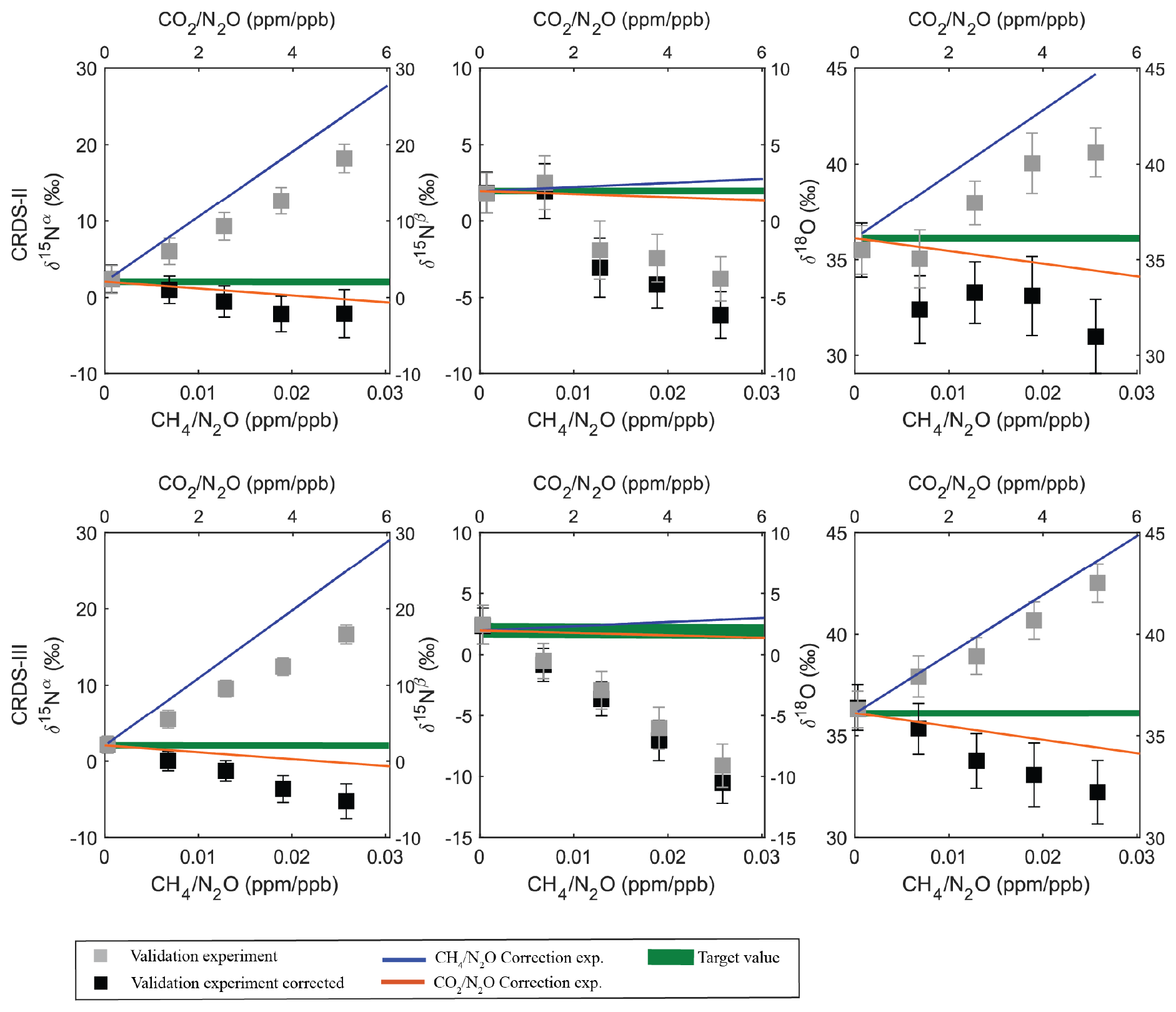
Figure 9 Interference effects of simultaneous CH₄ and CO₂ addition on apparent N₂O isotopic composition ($\mathit{\delta }{{}^{\mathrm{15}}\mathrm{N}}^{\mathit{\alpha }}$, $\mathit{\delta }{{}^{\mathrm{15}}\mathrm{N}}^{\mathit{\beta }}$, δ¹⁸O) as function of ${\mathrm{CH}}_{\mathrm{4}}/{\mathrm{N}}_{\mathrm{2}}\mathrm{O}$ (bottom x axis) and ${\mathrm{CO}}_{\mathrm{2}}/{\mathrm{N}}_{\mathrm{2}}\mathrm{O}$ (top x axis) concentration ratios. Measurements were conducted at stepwise increasing CH₄ and CO₂ but constant N₂O (330 ppb) concentration. Grey squares represent experimental data; i.e. apparent data not corrected for CH₄ and CO₂ effects on δ-values. Blue solid lines denote the experimentally determined correction functions for shifts in isotopic compositions with respect to ${\mathrm{CH}}_{\mathrm{4}}/{\mathrm{N}}_{\mathrm{2}}\mathrm{O}$ addition, only (Exp 2; Table 5). Likewise, the orange solid lines indicate experimentally determined correction functions for isotopic composition shifts with respect to ${\mathrm{CO}}_{\mathrm{2}}/{\mathrm{N}}_{\mathrm{2}}\mathrm{O}$ only (Exp. 3; Table 6). The green area represents N₂O isotopic compositions of the reference gas (Cal 1_90 ppm; $\mathit{\delta }{{}^{\mathrm{15}}\mathrm{N}}^{\mathit{\alpha }}=\mathrm{2.06}$ ‰ ± 0.05 ‰, $\mathit{\delta }{{}^{\mathrm{15}}\mathrm{N}}^{\mathit{\beta }}=\mathrm{1.98}$ ‰ ± 0.20 ‰, δ¹⁸O=36.12 ‰ ± 0.32 ‰). The black squares represent the δ-values corrected for CH₄ and CO₂ spectral interferences assuming additive effects of experimentally determined corrections. While for CH₄ inference correction analyser specific corrections were applied, for CO₂ interference correction, regression factors from CRDS-II were applied for both analysers. Each data point corresponds to the mean of up to three replicate measurements, where each replicate represents an average over 5 min. The indicated uncertainty represents the propagated standard error of individual 5 min measurements.

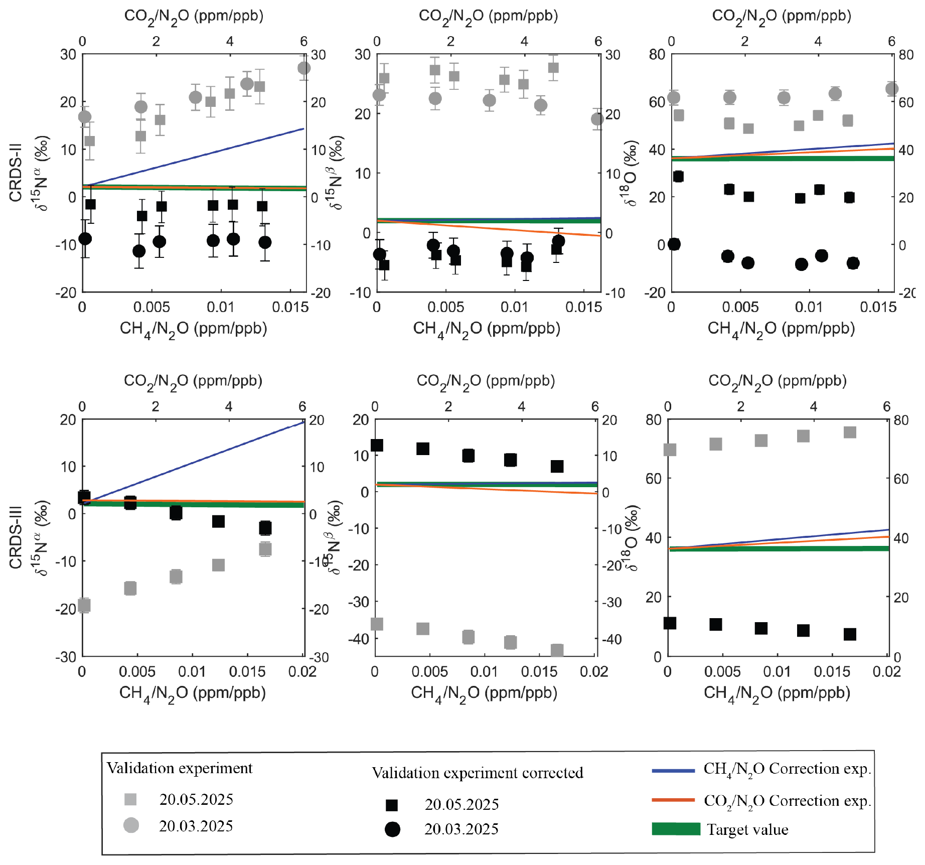
Figure 10 Interference effects of simultaneous changes in N₂O, CH₄ and CO₂, relative to reference gas composition on the apparent N₂O isotopic composition ($\mathit{\delta }{{}^{\mathrm{15}}\mathrm{N}}^{\mathit{\alpha }}$, $\mathit{\delta }{{}^{\mathrm{15}}\mathrm{N}}^{\mathit{\beta }}$, δ¹⁸O) as functions of ${\mathrm{CH}}_{\mathrm{4}}/{\mathrm{N}}_{\mathrm{2}}\mathrm{O}$ (bottom x axis) and ${\mathrm{CO}}_{\mathrm{2}}/{\mathrm{N}}_{\mathrm{2}}\mathrm{O}$ (top x axis) concentration ratios at constant N₂O (660 ppb). Grey squares represent experimental, i.e. apparent data not corrected for CH₄ and CO₂ effects on δ-values. The blue solid line denotes the experimentally determined correction function for shifts in isotopic compositions with respect to ${\mathrm{CH}}_{\mathrm{4}}/{\mathrm{N}}_{\mathrm{2}}\mathrm{O}$ mixtures without simultaneous addition of CO₂ (Exp. 2; Table 6). Likewise, the orange solid line indicates the experimentally determined correction function for isotopic composition shift with respect to ${\mathrm{CO}}_{\mathrm{2}}/{\mathrm{N}}_{\mathrm{2}}\mathrm{O}$ mixtures without concurrent addition of CH₄ (Exp. 3; Table 5). The green area represents N₂O isotopic compositions of the reference gas (Cal 1_90 ppm; $\mathit{\delta }{{}^{\mathrm{15}}\mathrm{N}}^{\mathit{\alpha }}=\mathrm{2.06}$ ‰ ± 0.05 ‰, $\mathit{\delta }{{}^{\mathrm{15}}\mathrm{N}}^{\mathit{\beta }}=\mathrm{1.98}$ ‰ ± 0.20 ‰, δ¹⁸O=36.12 ‰ ± 0.32 ‰). The black squares represent δ-values corrected for differences in N₂O, CH₄ and CO₂ concentrations, relative to reference gases, assuming additivity of interferences. For N₂O and CH₄ interference correction, analyser specific corrections were applied for CO₂ regression factors determined for CRDS-II were used for both analysers. Each data point corresponds to the mean of up to three replicate measurements, where each replicate represents an average over 5 min. The indicated uncertainty represents the propagated standard error of individual 5 min measurements.

Validation experiments carried out at 660 ppb N₂O show an even more complex interplay of interference effects (Fig. 10). Our working hypothesis was, that interferences by N₂O non-linearity and CH₄ as well as CO₂ spectral artifacts, induced by changes in N₂O, CH₄ and CO₂ concentrations of the sample relative to the reference gas, are additive. Experimental results (grey symbols) and δ-values corrected assuming additivity of interferences (black symbols) for CRDS-II display a consistent offset in delta values of up to 15 ‰ for $\mathit{\delta }{{}^{\mathrm{15}}\mathrm{N}}^{\mathit{\alpha }}$ and $\mathit{\delta }{{}^{\mathrm{15}}\mathrm{N}}^{\mathit{\beta }}$ but 20 ‰–40 ‰ for δ¹⁸O. In fact, two datasets were collected on two different measurement dates (20 March and 20 May 2025). The datasets were corrected using identical CH₄ and CO₂ regression factors but for the N₂O nonlinearity correction the correction function determined closest to the measurement date were applied (Table 4). Interestingly, measurements at 20 May 2025 (black squared symbols) were corrected with a N₂O non-linearity correction slope, which was determined just a few days before (16 May 2025), and resulted in a better agreement with target values than the second dataset, where N₂O non-linearity (10 April 2025) and validation measurements (20 March 2025) were separated by a longer time interval. For CRDS-III offsets are somewhat smaller for $\mathit{\delta }{{}^{\mathrm{15}}\mathrm{N}}^{\mathit{\alpha }}$ and $\mathit{\delta }{{}^{\mathrm{15}}\mathrm{N}}^{\mathit{\beta }}$ but indicate a decreasing trend with increasing CH₄ and CO₂ concentrations, similar to measurements at 330 ppb N₂O. Corrected results for δ¹⁸O analysed by CRDS-III show an approximately 25 ‰ offset. We speculate, that persistent offsets between corrected delta values to the target are linked to the observed changes in the N₂O non-linearity correction function over time (Fig. 5; Table 4).

4 Discussion

We implemented and parametrised the mathematical framework for the correction and calibration of N₂O isotopic data in a stand-alone MATLAB code. More specifically, output data of the CRDS analyser model G5131-i (Picarro Inc., USA) was used and corrections relevant for N₂O emissions from soils applied. The tested CRDS analyser model G5131-i has the potential for real-time analysis of the N₂O site-specific isotopic composition ($\mathit{\delta }{{}^{\mathrm{15}}\mathrm{N}}^{\mathit{\alpha }}$, $\mathit{\delta }{{}^{\mathrm{15}}\mathrm{N}}^{\mathit{\beta }}$) as well as δ¹⁸O in ambient N₂O at high precision (<1 ‰). To provide accurate data, relevant differences in gas composition between the sample and the applied isotope reference gases have to be assessed and, if necessary, corrected. It is best practice to adapt the gas composition of isotope reference gases to match the sample; however, most applications involve inevitable changes in gas concentrations, which must be either eliminated or considered. For the target application of this study, N₂O emissions from soil, changes in N₂O, CH₄, CO₂ and H₂O concentrations are expected to occur. The implemented correction terms for N₂O non-linearity, spectral interferences by CH₄, CO₂, gas matrix and drift effects and calibration to international isotope ratio scales are more widely applicable and in line with guidelines developed for other isotope systems (CO₂ and CH₄) and analyser models (Braden-Behrens et al., 2023; Sperlich et al., 2024). We tested the applicability of correction terms beyond a single analyser specimen and over time, comparing interference effects across three individual instruments, with published data for the G5131-i analyser model (Harris et al., 2020) and spectral simulations. Finally, the additivity of correction terms for interference effects was tested in a validation study for simultaneous changes in CH₄, CO₂, and N₂O concentrations. Different aspects of our study are discussed in more detail below.

4.1 Limitations and operational requirements for G5131-i

4.1.1 Non-additive behaviour of correction terms

Results of the first validation experiments (Fig. 9), in which CH₄ and CO₂ concentrations were changed simultaneously in sample gases with respect to isotopic reference gases, indicate that the spectral interference effects of CH₄ and CO₂ on apparent delta values are non-additive, which contradicts our prior assumption. Spectral interferences by changes in CH₄ concentration alone were found to be independent of the analyser specimen and constant over time, and therefore can be effectively corrected. Interestingly, experimentally determined CO₂ interferences were smaller than anticipated from spectral simulations, indicating that the raw data were post-corrected by the analyser software. We therefore speculate whether the presence of CH₄ may mislead the CO₂ post-correction algorithm implemented in the analyser software, resulting in the observed offsets. Alternatively, the presence of CO₂ may reduce spectral interferences from CH₄, thereby increasing absorption towards a non-linear regime in specific wavelength regions. The tested scenarios with up to 2000 ppm CO₂ and 10 ppm CH₄ changes might be realistic for some applications in the agricultural sector (e.g. dairy housing; Schrade et al., 2023) but are too strict for N₂O studies in upland soils, where CH₄ concentrations changes are substantially smaller (e.g. 50–300 ppb CH₄). If two or more relevant spectral interferents are present, we suggest avoiding additive spectral-interference correction, because it can lead to inaccurate results. Instead, interferants should be removed using adsorbents or catalysts, e.g. CO₂ by alkaline sorbents. The spectral interference of the residual interferant can then be corrected accurately. Alternatively, one might consider developing and implementing more complex two- or multi-dimensional interference correction schemes, which, however, is beyond the focus of our study.

4.1.2 Temporally variable N₂O non-linearity correction

Results of the second validation experiment (Fig. 10), conducted at 660 ppb N₂O, exhibit an even more complex interplay of N₂O non-linearity and CO₂ as well as CH₄ spectral interference. In fact, corrected measurement data for samples without CH₄ and CO₂ addition but only change in N₂O concentration (660 ppb as compared to 330 ppb for the reference gas), indicate in some cases agreement with the target composition within a few per mille but often more significant offsets. This discrepancy is most likely due to a drift in the N₂O non-linearity correction over time. The observed slopes represent the residual non-linearity after the Picarro Inc. G5131-i analyser built-in post-correction, whose parametrisation is instrument-specific, optimised before delivery, and can be updated by the manufacturer upon request. Since the internal algorithm is not disclosed, we cannot evaluate whether inter-instrument differences and the divergence of CRDS-III corrections from previous work (Harris et al., 2020) reflect differences in factory parametrisation, software updates, gradual changes in optical properties, or an interplay of these factors. Instrumental effects such as thermal fluctuations, minor pressure instabilities, or gradual mirror contamination may further contribute. Likewise, the Consultative Committee for Amount of Substance: Metrology in Chemistry and Biology (CCQM) Gas Analysis Working Group (GAWG) and Isotope Ratio Working Group (IRWG) suggests instrument developers to provide access to isotopologue raw data. Drift effects in N₂O non-linearity are indicated by replicate measurements over time for the same analyser specimen (Table 4). In addition, replicate measurements show better agreement of corrected data with target composition when correction parameters are determined shortly before or after the measurement sequence. Challenges with appropriate N₂O non-linearity correction are largest for δ¹⁸O, and less severe for $\mathit{\delta }{{}^{\mathrm{15}}\mathrm{N}}^{\mathit{\alpha }}$ and $\mathit{\delta }{{}^{\mathrm{15}}\mathrm{N}}^{\mathit{\beta }}$. Corrected results for samples with enhanced N₂O concentration as well as CH₄ and CO₂ concentrations, show a constant offset to target values, independent of CH₄ and CO₂ concentrations, for one analyser, while the second instrument shows an additional effect on non-additive CH₄ and CO₂ interference corrections. To ensure accurate N₂O isotopologue analysis using a G5131-i analyser, we recommend one of two alternative approaches. Either diluting the sample gas to ambient N₂O concentrations with full synthetic air (matrix c), thereby avoiding the need for a N₂O non-linearity correction, or analysing the N₂O non-linearity directly before/after each sample measurement sequence to ensure the correction function reflects the current instrumental conditions.

4.2 Recommendations and Best Practices for field measurements

In accordance with the results obtained from our study, we confirm the basic step-by-step workflow presented by Harris et al. (2020) for the G5131-i analyser but would like to refine several points, most importantly:

• The spectral interference on N₂O delta values measured by the CRDS analyser was found to be linearly dependent on the concentration of the spectral interferant (e.g. CH₄ or CO₂) and the inverse concentration of the target gas (N₂O).

• For the tested analyser model the CH₄ spectral interference on delta values was found to be of no significant difference for different analyser specimen, which would warrant the use of model specific correction terms. For post correction of delta values, parallel measurements with a specific CH₄ concentration analyser are required.

• Spectral interferences of different substances (e.g. CH₄ and CO₂) on N₂O δ-values were found to be non-additive, suggesting either removal of one interferant (e.g. CO₂) and correction of the second, or development of a more sophisticated correction model.

• The gas matrix effect of changes in the oxygen concentration on δ values was found to be independent of the N₂O target gas concentration, which simplifies corrections. Additivity of gas matrix effects and spectral interferences were not tested.

• N₂O non-linearity correction of delta values of the G5131-i analyser was found to be highly variable with time; we therefore suggest determining dependencies with a sufficiently high temporal resolution or diluting sample gases to ambient N₂O concentrations, covered by reference gases, using an appropriate dilution gas.

The established mathematical framework was implemented in a MATLAB code, parametrised and is applicable for other isotope systems or detection schemes but should be validated with care for the specific application before use.

4.3 Outlook and Future Work

A key outcome of this work is the development of a streamlined and easy-to-use post-processing protocol for isotopic data obtained on laser spectrometers in general and exemplified here by N₂O isotope data obtained with a G5131-i analyser from Picarro Inc. (USA). By combining analyser-specific N₂O non-linearity corrections with universally applicable corrections (e.g., CH₄) and by incorporating a GUM-compliant uncertainty analysis, we provide a stand-alone and user-friendly MATLAB post-processing routine for obtaining calibrated N₂O isotopic data. We suggest a future community effort to implement our workflow and accompanying MATLAB algorithm to ensure that N₂O isotope datasets generated at different laboratories are directly comparable and not affected by programming flaws. Furthermore, standardisation accelerates progress and therefore, this protocol can be used as a baseline while simultaneously updating the shared code as new analyser models, wavelength regions or calibration schemes emerge.

Future challenges lie in addressing the apparent non-additive interferences, such as the one observed between CH₄ and CO₂, where the combined effect of two interference gases on the δ-values cannot be predicted by simply summing up the individual correction terms. A key next step might be to characterise this behaviour systematically and potentially embed a dedicated CH₄–CO₂ interaction coefficient into the post-processing routine. Extending experimental investigations of non-additive effects to other interference gases, CH₄ and O₂, will further broaden the applicability of this protocol.

Finally, for long-term field deployment of analysers, the robustness of the post-processing protocol has to be tested outside a controlled laboratory setting. Although field operation inevitably introduces additional variability to the measurements, a thorough understanding of critical interferences and a standardised data-reduction workflow should make high-quality N₂O isotope measurements manageable under real-world conditions. This will provide valuable insights into the biogeochemical cycling of this potent greenhouse gas.

Appendix A: Mathematical formulation of the data processing algorithm

Here we report the mathematical equations used for all corrections implemented in the data analysis algorithm. The main parameters are the N₂O concentration ([N₂O]) and the δ-values of the different isotopologues ($\mathit{\delta }{{}^{\mathrm{15}}\mathrm{N}}^{\mathit{\alpha }}$, $\mathit{\delta }{{}^{\mathrm{15}}\mathrm{N}}^{\mathit{\beta }}$, δ¹⁸O) obtained from the G5131-i analyser, and the CH₄, CO and CO₂ concentrations ([CH₄], [CO], [CO₂]) from the G2401 analyser. Note that, for brevity, the corrections on apparent delta-values are expressed below for a generic isotopologue (δ), while all equations are applied to all three measured isotopologues ($\mathit{\delta }{{}^{\mathrm{15}}\mathrm{N}}^{\mathit{\alpha }}$, $\mathit{\delta }{{}^{\mathrm{15}}\mathrm{N}}^{\mathit{\beta }}$, δ¹⁸O).

A1 Pre-processing

First, the measurement intervals (plateau) are identified and labelled by gas type as described in Sect. 2.4.1, and all data are averaged to a user-defined integration time (e.g., 15 s). All data points outside the plateau intervals are discarded, and the mean and standard deviations are calculated for each interval and gas type according to Eqs. A1–A4. Superscripts Mean and Int_k indicate quantities calculated over the entire experimental sequence and an individual measurement interval (k), respectively. Subscript Sample indicates a generic gas sample, which can be either a reference gas (Cal 1, Cal 2) or a generic sample (e.g., Sample₁, Sample₂, etc.).

$$\begin{array}{}\text{(A1)}& {\displaystyle }\begin{array}{rl}{\mathit{\delta }}_{\text{Sample}}^{\text{Mean}}& ={\displaystyle \frac{\mathrm{1}}{N}}\sum _{i=\mathrm{1}}^N{\mathit{\delta }}_{\text{Sample},i}\\ & \text{where }i=\mathrm{1},\mathrm{\dots },N\text{ are all data points that}\\ & \text{belong to Sample gas}\end{array}\text{(A2)}& {\displaystyle }{\mathit{\sigma }}_{\text{Sample}}^{\text{Mean}}=\sqrt{{\displaystyle \frac{\mathrm{1}}{N-\mathrm{1}}}\sum _{i=\mathrm{1}}^N({\mathit{\delta }}_{\text{Sample},i}-{\mathit{\delta }}_{\text{Sample}}^{\text{Mean}}{)}^{\mathrm{2}}}\text{(A3)}& {\displaystyle }\begin{array}{rl}{\mathit{\delta }}_{\text{Sample}}^{{\text{Int}}_k}& ={\displaystyle \frac{\mathrm{1}}{K}}\sum _{j=\mathrm{1}}^K{\mathit{\delta }}_{\text{Sample},j}\\ & \text{where }j=\mathrm{1},\mathrm{\dots },K\text{ are all data points that}\\ & \text{belong to Interval }k\end{array}\text{(A4)}& {\displaystyle }{\mathit{\sigma }}_{\text{Sample}}^{\text{Int}}=\sqrt{{\displaystyle \frac{\mathrm{1}}{K-\mathrm{1}}}\sum _{j=\mathrm{1}}^K({\mathit{\delta }}_{\text{Sample},j}-{\mathit{\delta }}_{\text{Sample}}^{{\text{Int}}_k}{)}^{\mathrm{2}}}\end{array}$$

A2 Instrumental parameters

The raw data are checked for potential correlations with G5131-i instrumental parameters, particularly cell pressure (p_Cell), cell temperature (T_Cell), chiller temperature (T_Chiller), and P9 (i.e., back-mirror) temperature (T_P9), by means of a “correlation matrix” plot of [N₂O] and all δ-values against all instrumental parameters (including R² correlation coefficients) that can be generated by the code, allowing the user to easily identify anomalous correlation. In case a significant correlation is observed, [N₂O] and the δ-values can be corrected applying Eqs. (A5) and (A6), where Y represents one of the instrumental parameters listed above (p_Cell, T_Cell, T_Chiller, T_P9). The slope m of the correction function is determined by a linear fit between the apparent N₂O concentration (or δ-value) and the considered controlling parameter, recorded during anchor or calibration gas 1 (Cal 1) measurements.

$$\begin{array}{}\text{(A5)}& {\displaystyle }[{\mathrm{N}}_{\mathrm{2}}\mathrm{O}{]}_{\text{Sample}}=[{\mathrm{N}}_{\mathrm{2}}\mathrm{O}{]}_{\text{Sample}}^{\text{Raw}}-m_{\mathrm{1}}(Y_{\text{Sample}}-Y_{{\text{Cal}}_{\mathrm{1}}}^{\text{Mean}})\text{(A6)}& {\displaystyle }{\mathit{\delta }}_{\text{Sample}}={\mathit{\delta }}_{\text{Sample}}^{\text{Raw}}-m_{\mathrm{2}}(Y_{\text{Sample}}-Y_{{\text{Cal}}_{\mathrm{1}}}^{\text{Mean}})\end{array}$$

A3 Correction of concentration data

The concentration data are corrected (superscript Corr) and calibrated (superscript Calib) by a drift correction (Eqs. A7 and A8) and a calibration correction (Eqs. A9 and A10), where [X] represents either [N₂O], [CH₄], [CO] or [CO₂]. For each sample interval, the “offset” due to drift is calculated as the difference between the linear interpolation of the two nearest (bracketing) Cal 1 intervals (Int(+), Int(−)) and its mean value over all Cal 1 intervals. Consequently, all Cal 1 measurements are corrected to their mean value. The calibration can be either a one- or two-point calibration correction, depending on the number of available reference gases (Cal₂: calibration gas 2). Superscript True indicates the given “true” value of the reference gases.

$$\begin{array}{}\text{(A7)}& {\displaystyle }[X{]}_{\text{Sample}}^{\text{Corr}}=[X{]}_{\text{Sample}}^{\text{Raw}}-\mathrm{\Delta }[X{]}_{\text{Drift}}\text{(A8)}& {\displaystyle }\begin{array}{rl}\mathrm{\Delta }[X{]}_{\text{Drift}}& ={\displaystyle \frac{\left\{\begin{array}{c}[X{]}_{{\text{Cal}}_{\mathrm{1}}}^{\text{Int(–),Raw}}\cdot (t_{\text{Sample}}-t_{{\text{Cal}}_{\mathrm{1}}}^{\text{Int(–)}})\\ +[X{]}_{{\text{Cal}}_{\mathrm{1}}}^{\text{Int(+),Raw}}\cdot (t_{{\text{Cal}}_{\mathrm{1}}}^{\text{Int(+)}}-t_{\text{Sample}})\end{array}\right\}}{t_{{\text{Cal}}_{\mathrm{1}}}^{\text{Int(+)}}-t_{{\text{Cal}}_{\mathrm{1}}}^{\text{Int(–)}}}}\\ & -[X{]}_{{\text{Cal}}_{\mathrm{1}}}^{\text{Mean,Raw}}\end{array}\text{(A9)}& {\displaystyle }\begin{array}{rl}& [X{]}_{\text{Sample}}^{\text{Corr,Calib}}=\\ & \left\{\begin{array}{l}[X{]}_{\text{Sample}}^{\text{Corr}}-([X{]}_{{\text{Cal}}_{\mathrm{1}}}^{\text{Mean,Corr}}-[X{]}_{{\text{Cal}}_{\mathrm{1}}}^{\text{True}})\\ & \left(\text{1-point calibration}\right)\\ y_X\cdot \left(\right[X{]}_{\text{Sample}}^{\text{Corr}}-\left[X{]}_{{\text{Cal}}_{\mathrm{1}}}^{\text{Mean,Corr}}\right)+[X{]}_{{\text{Cal}}_{\mathrm{1}}}^{\text{True}}\\ & \left(\text{2-point calibration}\right)\end{array}\right.\end{array}\text{(A10)}& {\displaystyle }{y}_X={\displaystyle \frac{[X{]}_{{\text{Cal}}_{\mathrm{1}}}^{\text{True}}-[X{]}_{{\text{Cal}}_{\mathrm{2}}}^{\text{True}}}{[X{]}_{{\text{Cal}}_{\mathrm{1}}}^{\text{Mean,Corr}}-[X{]}_{{\text{Cal}}_{\mathrm{2}}}^{\text{Mean,Corr}}}}\end{array}$$

A4 Correction of δ-values

The raw δ-values retrieved by the spectrometer can be corrected and calibrated by the sequential application of the N₂O concentration (Eq. A12), CH₄ and CO₂ spectral interference corrections (Eqs. A13 and A14), drift correction (Eq. A15), and calibration correction (Eqs. A16 and A17). The slopes of the N₂O concentration and spectral interference corrections ($m_{{\mathrm{N}}_{\mathrm{2}}\mathrm{O}},m_{{\mathrm{CH}}_{\mathrm{4}}},m_{{\mathrm{CO}}_{\mathrm{2}}}$) are instrument-specific and must be defined by the user for each of the measured isotopologues (¹⁵N^α, ¹⁵N^β, ¹⁸O). Again, the calibration correction can be either a one- or two-point calibration, depending on the number of available reference gases

$$\begin{array}{}\text{(A11)}& {\displaystyle }\begin{array}{rl}{\mathit{\delta }}_{\text{Sample}}^{\text{Corr}}& ={\mathit{\delta }}_{\text{Sample}}^{\text{Raw}}-\mathrm{\Delta }{\mathit{\delta }}_{{\mathrm{N}}_{\mathrm{2}}\mathrm{O}}-\mathrm{\Delta }{\mathit{\delta }}_{{\mathrm{CH}}_{\mathrm{4}}}\\ & -\mathrm{\Delta }{\mathit{\delta }}_{{\mathrm{CO}}_{\mathrm{2}}}-\mathrm{\Delta }{\mathit{\delta }}_{\text{Drift}}\end{array}\text{(A12)}& {\displaystyle }\mathrm{\Delta }{\mathit{\delta }}_{{\mathrm{N}}_{\mathrm{2}}\mathrm{O}}=m_{{\mathrm{N}}_{\mathrm{2}}\mathrm{O}}\left({\displaystyle \frac{\mathrm{1}}{[{\mathrm{N}}_{\mathrm{2}}\mathrm{O}{]}_{\text{Sample}}^{\text{Corr,Calib}}}}-{\displaystyle \frac{\mathrm{1}}{[{\mathrm{N}}_{\mathrm{2}}\mathrm{O}{]}_{{\text{Cal}}_{\mathrm{1}}}^{\text{True}}}}\right)\text{(A13)}& {\displaystyle }\mathrm{\Delta }{\mathit{\delta }}_{{\mathrm{CH}}_{\mathrm{4}}}=m_{{\mathrm{CH}}_{\mathrm{4}}}\left({\displaystyle \frac{[{\mathrm{CH}}_{\mathrm{4}}{]}_{\text{Sample}}^{\text{Corr,Calib}}}{[{\mathrm{N}}_{\mathrm{2}}\mathrm{O}{]}_{\text{Sample}}^{\text{Corr,Calib}}}}-{\displaystyle \frac{[{\mathrm{CH}}_{\mathrm{4}}{]}_{{\text{Cal}}_{\mathrm{1}}}^{\text{True}}}{[{\mathrm{N}}_{\mathrm{2}}\mathrm{O}{]}_{{\text{Cal}}_{\mathrm{1}}}^{\text{True}}}}\right)\text{(A14)}& {\displaystyle }\mathrm{\Delta }{\mathit{\delta }}_{{\mathrm{CO}}_{\mathrm{2}}}=m_{{\mathrm{CO}}_{\mathrm{2}}}\left({\displaystyle \frac{[{\mathrm{CO}}_{\mathrm{2}}{]}_{\text{Sample}}^{\text{Corr,Calib}}}{[{\mathrm{N}}_{\mathrm{2}}\mathrm{O}{]}_{\text{Sample}}^{\text{Corr,Calib}}}}-{\displaystyle \frac{[{\mathrm{CO}}_{\mathrm{2}}{]}_{{\text{Cal}}_{\mathrm{1}}}^{\text{True}}}{[{\mathrm{N}}_{\mathrm{2}}\mathrm{O}{]}_{{\text{Cal}}_{\mathrm{1}}}^{\text{True}}}}\right)\text{(A15)}& {\displaystyle }\begin{array}{rl}\mathrm{\Delta }{\mathit{\delta }}_{\text{Drift}}& ={\displaystyle \frac{\left\{\begin{array}{c}{\mathit{\delta }}_{{\text{Cal}}_{\mathrm{1}}}^{\text{Int(–),Raw}}\cdot (t_{\text{Sample}}-t_{{\text{Cal}}_{\mathrm{1}}}^{\text{Int(–)}})\\ +{\mathit{\delta }}_{{\text{Cal}}_{\mathrm{1}}}^{\text{Int(+),Raw}}\cdot (t_{{\text{Cal}}_{\mathrm{1}}}^{\text{Int(+)}}-t_{\text{Sample}})\end{array}\right\}}{t_{{\text{Cal}}_{\mathrm{1}}}^{\text{Int(+)}}-t_{{\text{Cal}}_{\mathrm{1}}}^{\text{Int(–)}}}}\\ & -{\mathit{\delta }}_{{\text{Cal}}_{\mathrm{1}}}^{\text{Mean,Raw}}\end{array}\text{(A16)}& {\displaystyle }\begin{array}{rl}& {\mathit{\delta }}_{\text{Sample}}^{\text{Corr,Calib}}=\\ & \left\{\begin{array}{l}{\mathit{\delta }}_{\text{Sample}}^{\text{Corr}}-({\mathit{\delta }}_{{\text{Cal}}_{\mathrm{1}}}^{\text{Mean,Corr}}-{\mathit{\delta }}_{{\text{Cal}}_{\mathrm{1}}}^{\text{True}})\\ & \mathrm{\text{(1-point calibration)}}\\ y\cdot ({\mathit{\delta }}_{\text{Sample}}^{\text{Corr}}-{\mathit{\delta }}_{{\text{Cal}}_{\mathrm{1}}}^{\text{Mean,Corr}})+{\mathit{\delta }}_{{\text{Cal}}_{\mathrm{1}}}^{\text{True}}\\ & \mathrm{\text{(2-point calibration)}}\end{array}\right.\end{array}\text{(A17)}& {\displaystyle }y={\displaystyle \frac{{\mathit{\delta }}_{{\text{Cal}}_{\mathrm{1}}}^{\text{True}}-{\mathit{\delta }}_{{\text{Cal}}_{\mathrm{2}}}^{\text{True}}}{{\mathit{\delta }}_{{\text{Cal}}_{\mathrm{1}}}^{\text{Mean,Corr}}-{\mathit{\delta }}_{{\text{Cal}}_{\mathrm{2}}}^{\text{Mean,Corr}}}}\end{array}$$

A5 Uncertainty propagation

Finally, the code offers the possibility to calculate the propagated uncertainty (u) on the final δ-values associated with all the applied corrections and calibration, using the error propagation law (Eqs. A18 and A19). Five error sources (U) are considered and must be defined by the user for each isotopologue, including uncertainties in the slopes used for the N₂O concentration correction and spectral interference corrections ($m_{{\mathrm{N}}_{\mathrm{2}}\mathrm{O}},m_{{\mathrm{CH}}_{\mathrm{4}}},m_{{\mathrm{CO}}_{\mathrm{2}}}$), uncertainties in the “true” δ-values attributed to reference gases (${\mathit{\delta }}_{{\text{Cal}}_{\mathrm{1}}}^{\text{True}},{\mathit{\delta }}_{{\text{Cal}}_{\mathrm{2}}}^{\text{True}}$), plus an additional term representing “poorly understood” effects (u_Other), which can be approximated by repeatability for target gas measurements.

$$\begin{array}{}\text{(A18)}& {\displaystyle }U=(m_{{\mathrm{N}}_{\mathrm{2}}\mathrm{O}},m_{{\mathrm{CH}}_{\mathrm{4}}},m_{{\mathrm{CO}}_{\mathrm{2}}},{\mathit{\delta }}_{{\text{Cal}}_{\mathrm{1}}}^{\text{True}},{\mathit{\delta }}_{{\text{Cal}}_{\mathrm{2}}}^{\text{True}})\text{(A19)}& {\displaystyle }{u}_{\text{Sample}}^{\text{Corr,Calib}}=\sqrt{\sum _{i=\mathrm{1}}^{\mathrm{5}}{\left({\displaystyle \frac{\partial {\mathit{\delta }}_{\text{Sample}}^{\text{Corr,Calib}}}{\partial U_{\mathrm{i}}}}\mathrm{\Delta }{U}_{\mathrm{i}}\right)}^{\mathrm{2}}+u_{\text{Other}}^{\mathrm{2}}}\end{array}$$

Solving the partial derivatives of Eq. (A19) for a 2-point calibration correction (see Eq. A16) yields:

$$\begin{array}{}\text{(A20)}& {\displaystyle }\begin{array}{rl}{\displaystyle \frac{\partial {\mathit{\delta }}_{\text{Sample}}^{\text{Corr,Calib}}}{\partial m_{{\mathrm{N}}_{\mathrm{2}}\mathrm{O}}}}& \mathrm{\Delta }{m}_{{\mathrm{N}}_{\mathrm{2}}\mathrm{O}}=\\ & y\left({\displaystyle \frac{\mathrm{1}}{[{\mathrm{N}}_{\mathrm{2}}\mathrm{O}{]}_{\text{Sample}}^{\text{Corr,Calib}}}}-{\displaystyle \frac{\mathrm{1}}{[{\mathrm{N}}_{\mathrm{2}}\mathrm{O}{]}_{{\text{Cal}}_{\mathrm{1}}}^{\text{True}}}}\right)\mathrm{\Delta }{m}_{{\mathrm{N}}_{\mathrm{2}}\mathrm{O}}\end{array}\text{(A21)}& {\displaystyle }\begin{array}{rl}{\displaystyle \frac{\partial {\mathit{\delta }}_{\text{Sample}}^{\text{Corr,Calib}}}{\partial m_{{\mathrm{CH}}_{\mathrm{4}}}}}& \mathrm{\Delta }{m}_{{\mathrm{CH}}_{\mathrm{4}}}=\\ & y\left({\displaystyle \frac{[{\mathrm{CH}}_{\mathrm{4}}{]}_{\text{Sample}}^{\text{Corr,Calib}}}{[{\mathrm{N}}_{\mathrm{2}}\mathrm{O}{]}_{\text{Sample}}^{\text{Corr,Calib}}}}-{\displaystyle \frac{[{\mathrm{CH}}_{\mathrm{4}}{]}_{{\text{Cal}}_{\mathrm{1}}}^{\text{True}}}{[{\mathrm{N}}_{\mathrm{2}}\mathrm{O}{]}_{{\text{Cal}}_{\mathrm{1}}}^{\text{True}}}}\right)\mathrm{\Delta }{m}_{{\mathrm{CH}}_{\mathrm{4}}}\end{array}\text{(A22)}& {\displaystyle }\begin{array}{rl}{\displaystyle \frac{\partial {\mathit{\delta }}_{\text{Sample}}^{\text{Corr,Calib}}}{\partial m_{{\mathrm{CO}}_{\mathrm{2}}}}}& \mathrm{\Delta }{m}_{{\mathrm{CO}}_{\mathrm{2}}}=\\ & y\left({\displaystyle \frac{[{\mathrm{CO}}_{\mathrm{2}}{]}_{\text{Sample}}^{\text{Corr,Calib}}}{[{\mathrm{N}}_{\mathrm{2}}\mathrm{O}{]}_{\text{Sample}}^{\text{Corr,Calib}}}}-{\displaystyle \frac{[{\mathrm{CO}}_{\mathrm{2}}{]}_{{\text{Cal}}_{\mathrm{1}}}^{\text{True}}}{[{\mathrm{N}}_{\mathrm{2}}\mathrm{O}{]}_{{\text{Cal}}_{\mathrm{1}}}^{\text{True}}}}\right)\mathrm{\Delta }{m}_{{\mathrm{CO}}_{\mathrm{2}}}\end{array}\text{(A23)}& {\displaystyle }\begin{array}{rl}{\displaystyle \frac{\partial {\mathit{\delta }}_{\text{Sample}}^{\text{Corr,Calib}}}{\partial {\mathit{\delta }}_{{\text{Cal}}_{\mathrm{1}}}^{\text{True}}}}& \mathrm{\Delta }{\mathit{\delta }}_{{\text{Cal}}_{\mathrm{1}}}^{\text{True}}=\\ & \left({\displaystyle \frac{{\mathit{\delta }}_{\text{Sample}}^{\text{Corr}}-{\mathit{\delta }}_{{\text{Cal}}_{\mathrm{2}}}^{\text{Mean,Corr}}}{{\mathit{\delta }}_{{\text{Cal}}_{\mathrm{1}}}^{\text{Mean,Corr}}-{\mathit{\delta }}_{{\text{Cal}}_{\mathrm{2}}}^{\text{Mean,Corr}}}}\right)\mathrm{\Delta }{\mathit{\delta }}_{\text{Cal1}}\end{array}\text{(A24)}& {\displaystyle }\begin{array}{rl}{\displaystyle \frac{\partial {\mathit{\delta }}_{\text{Sample}}^{\text{Corr,Calib}}}{\partial {\mathit{\delta }}_{{\text{Cal}}_{\mathrm{2}}}^{\text{True}}}}& \mathrm{\Delta }{\mathit{\delta }}_{{\text{Cal}}_{\mathrm{2}}}^{\text{True}}=\\ & \left({\displaystyle \frac{{\mathit{\delta }}_{{\text{Cal}}_{\mathrm{1}}}^{\text{Mean,Corr}}-{\mathit{\delta }}_{\text{Sample}}^{\text{Corr}}}{{\mathit{\delta }}_{{\text{Cal}}_{\mathrm{1}}}^{\text{Mean,Corr}}-{\mathit{\delta }}_{{\text{Cal}}_{\mathrm{2}}}^{\text{Mean,Corr}}}}\right)\mathrm{\Delta }{\mathit{\delta }}_{{\text{Cal}}_{\mathrm{2}}}\end{array}\end{array}$$

Solving the partial derivatives of Eq. (A19) for a 1-point calibration correction (i.e., $\mathrm{\Delta }{\mathit{\delta }}_{{\text{Cal}}_{\mathrm{2}}}^{\text{True}}=\mathrm{0}$) yields:

$$\begin{array}{}\text{(A25)}& {\displaystyle }\begin{array}{rl}{\displaystyle \frac{\partial {\mathit{\delta }}_{\text{Sample}}^{\text{Corr,Calib}}}{\partial m_{{\mathrm{N}}_{\mathrm{2}}\mathrm{O}}}}& \mathrm{\Delta }{m}_{{\mathrm{N}}_{\mathrm{2}}\mathrm{O}}=\\ & \left({\displaystyle \frac{\mathrm{1}}{[{\mathrm{N}}_{\mathrm{2}}\mathrm{O}{]}_{\text{Sample}}^{\text{Corr,Calib}}}}-{\displaystyle \frac{\mathrm{1}}{[{\mathrm{N}}_{\mathrm{2}}\mathrm{O}{]}_{{\text{Cal}}_{\mathrm{1}}}^{\text{True}}}}\right)\mathrm{\Delta }{m}_{{\mathrm{N}}_{\mathrm{2}}\mathrm{O}}\end{array}\text{(A26)}& {\displaystyle }\begin{array}{rl}{\displaystyle \frac{\partial {\mathit{\delta }}_{\text{Sample}}^{\text{Corr,Calib}}}{\partial m_{{\mathrm{CH}}_{\mathrm{4}}}}}& \mathrm{\Delta }{m}_{{\mathrm{CH}}_{\mathrm{4}}}=\\ & \left({\displaystyle \frac{[{\mathrm{CH}}_{\mathrm{4}}{]}_{\text{Sample}}^{\text{Corr,Calib}}}{[{\mathrm{N}}_{\mathrm{2}}\mathrm{O}{]}_{\text{Sample}}^{\text{Corr,Calib}}}}-{\displaystyle \frac{[{\mathrm{CH}}_{\mathrm{4}}{]}_{{\text{Cal}}_{\mathrm{1}}}^{\text{True}}}{[{\mathrm{N}}_{\mathrm{2}}\mathrm{O}{]}_{{\text{Cal}}_{\mathrm{1}}}^{\text{True}}}}\right)\mathrm{\Delta }{m}_{{\mathrm{CH}}_{\mathrm{4}}}\end{array}\text{(A27)}& {\displaystyle }\begin{array}{rl}{\displaystyle \frac{\partial {\mathit{\delta }}_{\text{Sample}}^{\text{Corr,Calib}}}{\partial m_{{\mathrm{CO}}_{\mathrm{2}}}}}& \mathrm{\Delta }{m}_{{\mathrm{CO}}_{\mathrm{2}}}=\\ & \left({\displaystyle \frac{[{\mathrm{CO}}_{\mathrm{2}}{]}_{\text{Sample}}^{\text{Corr,Calib}}}{[{\mathrm{N}}_{\mathrm{2}}\mathrm{O}{]}_{\text{Sample}}^{\text{Corr,Calib}}}}-{\displaystyle \frac{[{\mathrm{CO}}_{\mathrm{2}}{]}_{{\text{Cal}}_{\mathrm{1}}}^{\text{True}}}{[{\mathrm{N}}_{\mathrm{2}}\mathrm{O}{]}_{{\text{Cal}}_{\mathrm{1}}}^{\text{True}}}}\right)\mathrm{\Delta }{m}_{{\mathrm{CO}}_{\mathrm{2}}}\end{array}\text{(A28)}& {\displaystyle \frac{\partial {\mathit{\delta }}_{\text{Sample}}^{\text{Corr,Calib}}}{\partial {\mathit{\delta }}_{{\text{Cal}}_{\mathrm{1}}}^{\text{True}}}}\mathrm{\Delta }{\mathit{\delta }}_{{\text{Cal}}_{\mathrm{1}}}^{\text{True}}=\mathrm{\Delta }{\mathit{\delta }}_{{\text{Cal}}_{\mathrm{1}}}\end{array}$$