Continuing the MLS water vapor record with OMPS LP using neural networks

Stratospheric water vapor (SWV) plays an important role in atmospheric chemistry, dynamics, and radiative forcing. Satellite measurements by the Aura Microwave Limb Sounder (MLS), SciSat-1 Atmospheric Chemistry Experiment Fourier Transform Spectrometer (ACE-FTS), and Stratospheric Aerosol and Gas Experiment III on the International Space Station (SAGE III/ISS) have provided key constraints on SWV for the past decades. MLS provides the best geographical coverage among these instruments, but it approaches the end of its life cycle in the coming years, which will result in a data desert for satellite-based SWV measurements given that ACE-FTS and SAGE III/ISS only measure at a few dozen geolocations per day. The Ozone Mapping and Profiler Suite Limb Profiler (OMPS LP) is flying aboard the Suomi National Polar-orbiting Partnership (SNPP) and NOAA-21 satellites and is planned for additional platforms in the coming years. While not designed to measure SWV, it shows weak sensitivity to it, particularly in the wake of the Hunga eruption's significant injection of water vapor into the stratosphere. By utilizing the frequent co-locations between OMPS LP and MLS measurements, we developed a neural network-based retrieval algorithm to estimate SWV from SNPP OMPS LP radiances between 11.5 and 40.5 km. We find that the LP SWV profiles typically agree with MLS within 5 %, and agreement with ACE-FTS and SAGE III/ISS is typically within 10 %. We show that the SNPP-trained model is applicable to NOAA-21 OMPS LP without retraining, though minor differences in radiances between the instruments results in a ∼ 5 % bias under most conditions. Our results suggest that OMPS LP can continue the global water vapor record in the lower stratosphere into the 2030s, though continued independent measurements by satellite and balloon-borne instruments will be key to verifying the stability of our approach for quantifying decadal-scale SWV variability.

1 Introduction

Stratospheric water vapor (SWV) influences atmospheric dynamics, chemistry, and radiative forcing (e.g., Ramanathan and Inamdar, 2006; Charlesworth et al., 2023; Niemeier et al., 2023; Fleming et al., 2024). While SWV is typically 3–6 parts per million by volume (ppmv), water vapor concentrations in the upper troposphere can reach up to 1000 ppmv (e.g., Read et al., 2022). Deep convective systems and tropical upwelling via the Brewer–Dobson circulation can transport tropospheric air into the lower stratosphere, which comprises an important contribution to SWV (e.g., Fueglistaler et al., 2009; Khaykin et al., 2009; Randel and Jensen, 2013; Dauhut et al., 2016). Rising atmospheric temperature due to climate change increases the amount of water vapor held in tropospheric air, which in turn increases the amount of water vapor transported into the stratosphere (Yue et al., 2019; Nowack et al., 2023). Long-term satellite measurements of SWV provide key constraints on the SWV budget and serve as important sources for data assimilation and validation of reanalysis frameworks (e.g., Davis et al., 2017; Hersbach et al., 2020; Wargan et al., 2023; Knowland et al., 2025).

Presently, satellite retrievals of SWV profiles are performed by the Aura Microwave Limb Sounder (MLS; Waters et al., 2006; Livesey et al., 2021), SciSat-1 Atmospheric Chemistry Experiment Fourier Transform Spectrometer (ACE-FTS; Bernath et al., 2005; Boone et al., 2023), Stratospheric Aerosol and Gas Experiment III aboard the International Space Station (SAGE III/ISS; Cisewski et al., 2014), and the Thermosphere Ionosphere Mesosphere Energetics Dynamics (TIMED) satellite's Sounding of the Atmosphere using Broadband Emission Radiometry (SABER; Russell et al., 1999) instruments. These instruments provide well validated H₂O products that typically show median differences within ∼ 10 % among each other as well as with ground-based and in-situ measurements (e.g., Carleer et al., 2008; Hurst et al., 2014; Rong et al., 2019; Davis et al., 2021; Park et al., 2021; De Los Ríos et al., 2024). Since May 2024, the MLS receiver used for the H₂O retrievals now only operates around 6 d per month to preserve measurement lifetime and will continue to do so until the end of the Aura mission, which significantly limits the spatiotemporal coverage of the MLS H₂O product. Following the decommissioning of Aura, ACE-FTS and SAGE III/ISS will continue to provide their H₂O products, but their geographical coverage is limited given they are solar occultation instruments. SABER takes around 1400 scans per day and, depending on time of year, views between 52° S–83° N or 83° S–52° N; the local times of the measurements change by up to 12 h over TIMED's 2-month yaw cycle. The Canadian High-altitude Aerosols, Water vapour, and Clouds mission (HAWC; Langille et al., 2025) is planned to launch early next decade, presenting a gap in global geographical coverage of SWV between Aura's decommissioning and HAWC's launch (Salawitch et al., 2025).

The Ozone Mapping and Profiler Suite (OMPS) Limb Profiler (LP; Dittman et al., 2002; Leitch et al., 2003) is currently flying aboard the Suomi National Polar-orbiting Partnership (SNPP; launched 28 October 2011) and NOAA-21 (launched 10 November 2022) satellites, and it is planned for the Joint Polar Satellite System (JPSS) 4 and 3 satellites, which are estimated to launch in 2027 and 2032, respectively. Using 3 slits, the instrument measures limb-scattered radiances between 290 and 1000 nm with a 1 km vertical sampling. Each satellite completes 14–15 Sun-synchronous orbits per day. SNPP's OMPS LP takes measurements every ∼ 1° latitude, while NOAA-21's LP takes measurements every ∼ 0.4° latitude, resulting in around 7000 and 17 500 measured radiance profiles per day, respectively. However, OMPS LP is only weakly sensitive to H₂O, which has challenged the application of traditional radiative transfer-based retrieval methods.

Our solution to retrieve water vapor profiles from OMPS LP measurements is deep learning (Goodfellow et al., 2016). Neural networks (NNs) learn to model complex, nonlinear processes in a data-driven manner. Given a set of corresponding inputs and outputs, the NN weights are tuned to approximate the underlying process, without explicit knowledge about it. Given OMPS LP's weak sensitivity to H₂O and the well validated MLS H₂O product, NNs could learn to accurately predict H₂O profiles from OMPS LP measurements at altitudes with sufficient sensitivity by using co-located MLS H₂O profiles as the target outputs. This would result in an MLS-like H₂O product, thereby continuing the MLS global SWV record following the end of the Aura mission.

Here we present an OMPS LP water vapor product between 11.5 and 40.5 km produced by a NN trained on co-located LP-MLS measurements. In Sect. 2 we investigate the sensitivity of LP to water vapor under conditions before and after the Hunga Tonga–Hunga Ha'apai (hereafter Hunga) eruption, which injected more than 50 Tg of water into the stratosphere (e.g., Millán et al., 2022; Vömel et al., 2022; Khaykin et al., 2022; APARC, 2025). In Sec. 3 we discuss our methodology to train the NN as well as validate its predictions using other instruments. We present and discuss our results in Sect. 4, including the limitations of our approach. Finally, we present our conclusions in Sect. 5.

2 OMPS LP sensitivity to H₂O

We investigate OMPS LP's H₂O sensitivity using the Gauss–Seidel limb scattering (GSLS) radiative transfer model (RTM) (see Herman et al., 1994; Loughman et al., 2004, 2005, 2015). To calculate H₂O cross sections, we use the HITRAN 2020 database (Gordon et al., 2022) via the HITRAN Application Programming Interface (Kochanov et al., 2016). We then convolve those high-resolution cross sections with the OMPS LP bandpasses such that RTM calculations at a given wavelength will be more consistent with what LP would measure for the assumed conditions. Using two selected co-located MLS H₂O profiles from before and after the Hunga eruption, we simulate radiances between 550 and 1025 nm in 5 nm intervals at altitudes of 3.5–50.5 km in 1 km intervals. For the two RTM simulations, all parameters are kept identical except for the H₂O profile ensuring that any differences in the Jacobians are due solely to variations in H₂O.

Based on the Jacobians output by the RTM, we select 12 wavelengths measured by OMPS LP (554, 596, 654, 720, 728, 824, 917, 929, 943, 956, 970, and 983 nm) that show the highest sensitivity to H₂O in their spectral region. Figure 1 shows an example of these Jacobians at 945 nm for the selected H₂O profile after the Hunga eruption. The H₂O enhancement between 20 and 30 km attributable to the Hunga eruption results in as much as a four times increase in LP's sensitivity to H₂O. However, LP is very weakly sensitive to H₂O, and the sensitivity becomes negligible above 30 km. For more details on LP's sensitivity to H₂O, see Appendix A.

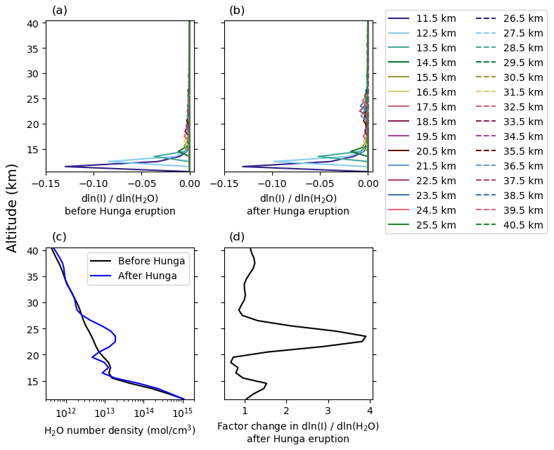
Figure 1 Example of OMPS LP's sensitivity to H₂O at 945 nm in the tropics. Panels (a) and (b) show the Jacobians for selected MLS H₂O profiles from before and after the Hunga eruption, respectively. Panel (c) shows the selected water vapor profiles, which show an enhancement in water vapor around 24 km attributable to the Hunga eruption. Panel (d) shows the ratio of panels (b) to (a). The increased water vapor concentration between 21 and 27 km due to Hunga results in LP's sensitivity increasing by up to 4 × in this altitude range.

3 Deep learning methods

3.1 Data curation

Since there is currently no water vapor product derived from OMPS LP measurements, we instead use the MLS version 5 water vapor product as our ground truth. To prioritize times where SNPP and Aura have closely aligned orbits, we select dates that have

• at least one orbit with 60 consecutive co-locations that are within 30 min and within 100 km, and

• at least 250 total co-locations on that day that satisfy the above co-location criteria.

These criteria are satisfied every couple days due to their similar equatorial crossing times around 13:30 in the afternoon. On dates between February 2014 and December 2024 that satisfy the above criteria, we co-locate OMPS LP and MLS measurements within 6 h and 100 km to build a data set of OMPS LP radiances and the corresponding MLS water vapor profiles. This results in 2 074 101 co-locations, with almost half occurring at high latitudes. For context, SNPP OMPS LP measures over 2.5 million vertical profiles per year.

We apply the recommended MLS data screening criteria except for the period of 15 January–12 February 2022, as it has been shown that the recommended screening criteria filter out many valid profiles affected by Hunga (Millán et al., 2024). We limit the MLS water vapor profiles to ≤ 261 hPa. We log-linearly interpolate the water vapor profiles from the MLS pressure grid to OMPS LP's geometric height (11.5–40.5 km in 1 km steps) using the NASA Global Earth Observing System Forward Processing for Instrument Teams (GEOS FP-IT; Lucchesi, 2015) pressures interpolated in time and space to the LP measurements. We limit the altitude range to 11.5–40.5 km because 10.5 km can exceed 261 hPa and the H₂O sensitivity of OMPS LP becomes ∼ 0 above 40.5 km.

We also consider a similar methodology for ACE-FTS and SAGE III/ISS data with recommended screening criteria applied to both datasets. We utilize co-location criteria of within 1 d, within 2° latitude, and within 1113 km longitude (equal to 10° longitude at the equator), consistent with the criteria used in Davis et al. (2021). These data sets are used to investigate whether it is viable to train exclusively on ACE-FTS or SAGE III/ISS data and whether training on a combination of MLS, ACE-FTS, and/or SAGE III/ISS data offers benefits over only training on MLS data.

3.2 Neural network methods

For each co-located measurement, we construct an input–output pair to be used during NN training. The inputs are comprised of

• LP radiances at 554, 596, 654, 720, 728, 824, 917, 929, 943, 956, 970, and 983 nm,

• GEOS FP-IT pressures and temperatures interpolated in time and space to the LP measurements, and

• the solar zenith angle of the LP measurement.

These inputs are formatted as 2-D “images” (wavelength × altitude) with four channels (radiance, pressure, temperature, solar zenith angle), similar to a standard RGBA image. The radiances vary at each point in the 2-D image, the pressures and temperatures vary only with respect to altitude, and the solar zenith angle is constant throughout. For each input image, the corresponding outputs are the co-located MLS H₂O profile that has been interpolated to the LP altitude grid. See Appendix B for a discussion of the relative importance of these inputs.

To address the latitudinal sampling bias inherent in the co-located data set, we first select a subset of the data such that there are roughly the same number of samples in each 5° latitudinal bin, resulting in 1 137 100 input–output pairs. We ensure that extrema for each latitudinal bin are included in this subset. We then split these data into training (used to update NN weights), validation (monitors for overfitting during training), and testing (tests model generality on unseen data after training is complete) sets in a proportion of roughly 75 %, 15 %, and 10 %, respectively. For context, this results in the training and validation sets containing a total of ∼ 3.7 % of all available SNPP OMPS LP data over the 2014–2024 period considered.

To investigate how the training data impacts the algorithm's ability to generalize to unseen data, we run additional experiments where certain years are omitted from the training data set. One test omits 2015–2016, which exhibits typical SWV, while the other test omits 2024, which contains SWV perturbations from Hunga.

For data pre-processing and NN training, we utilize the open-source Python package MARGE (Himes et al., 2022), which uses TensorFlow (Abadi et al., 2016) via the Keras API. We pre-process the data by taking the base-10 logarithm of the OMPS LP radiances, GEOS FP-IT pressures, and MLS H₂O profiles, then scale each input and output parameter to be within the closed interval $[-\mathrm{1},\mathrm{1}]$ based on their training set extrema at each altitude.

To determine a neural network architecture well suited to solving this problem, we perform a Bayesian hyperparameter optimization (Akiba et al., 2019). The selected architecture is similar to the landmark AlexNet architecture (Krizhevsky et al., 2012); for details on our optimization procedure, the selected architecture, and the training details, see Appendix C. Using the chosen architecture, we train an ensemble of 10 neural networks using a mean-squared-error (MSE) loss function; members are only differentiated by their random initialization. The ensemble size is held constant for all retrievals; it was determined by adding ensemble members until the mean and standard deviation of the ensemble's predictions did not significantly change. The ensemble's mean prediction provides the retrieved H₂O profile. The standard deviation among the ensemble provides an uncertainty estimate for the NNs' prediction of the MLS H₂O profile. MLS profiles also have some uncertainty; we factor this into the LP uncertainty estimate by combining these sources in quadrature, assuming that they are uncorrelated:

$$\begin{array}{}\text{(1)}& {\mathit{\sigma }}_{\mathrm{LP}}^{\mathrm{2}}={\mathit{\sigma }}_{\mathrm{NN}}^{\mathrm{2}}+{\mathit{\sigma }}_{\mathrm{MLS}}^{\mathrm{2}}\end{array}$$

We assume these terms are uncorrelated given that LP's errors at the wavelengths considered are dominated by systematics, and these should be unrelated to any random or systematic errors in the MLS data; this assumption has a negligible effect on the resulting LP uncertainty, as discussed in Sect. 4.1. Typically, σ_NN is small in the stratosphere due to close agreement among the NNs, leading the total LP uncertainties to be dominated by σ_MLS in this regime. In the troposphere, where strong scattering limits the NNs' accuracy, the LP uncertainties are dominated by σ_NN. We estimate the MLS uncertainty by computing 5° monthly zonal means at each pressure level considered for the reported MLS uncertainties over the 2015–2019 period. The chosen time period is a minor consideration, as the MLS data quality and description document reports that other time periods are similar to their reported January–March 2009 period (Livesey et al., 2022). These seasonal uncertainties are then log-linearly interpolated in time and pressure to the LP altitude grid using the GEOS-IT pressure data.

Additionally, we apply these methods to permutations of the co-located MLS, ACE-FTS, and/or SAGE III/ISS data sets. When combining more than one data set, we consider two approaches, one where we use the data as is, and another where we bias correct the ACE-FTS and SAGE III/ISS data such that they have a global median difference of 0 % at all altitudes with respect to MLS.

3.3 Evaluation and validation

To evaluate the NN's typical accuracy and how well it generalizes to unseen data, we calculate the root mean square error (RMSE) and coefficient of determination (R²) for the validation and test sets. We validate our LP water vapor product by comparing with satellite measurements, balloon-borne measurements, and an assimilation/reanalysis product.

For satellite measurements, we consider the MLS version 5 (Lambert et al., 2020), SAGE III/ISS version 6 (NASA/LARC/SD/ASDC, 2025), and ACE-FTS version 5.3 (Boone et al., 2023) products. For MLS, we consider co-locations within 6 h, while for SAGE III/ISS and ACE-FTS we consider co-locations within 24 h. For all three, we only consider the co-location if it is separated by less than 1000 km and within 2° latitude. When multiple co-locations satisfy these criteria, we use the co-location with the shortest distance. For each of these instruments, we compute both a global median percent difference as well as zonal median percent differences in 5° latitude bins. We found anomalous values in the SAGE III/ISS and ACE-FTS data sets that differ by a factor of up to 10 000 compared with the layers above and below it, even after applying each product's recommended screening criteria. To screen out the most extreme of these unrealistic values, we apply a very conservative 20σ median rejection routine to the data set of percent differences.

We investigate whether our product shows similar properties as the MLS product by performing a multiple linear regression (MLR) on monthly means for a 5° × 5° grid, with proxies for a linear trend, seasonal cycle, quasi-biennial oscillation (QBO), and El Niño Southern Oscillation (ENSO), as these terms explain the majority of stratospheric H₂O variability. For the seasonal cycle term, we also include a phase offset term for lag in months, given that it takes time for the effects to propagate upwards through the stratosphere. For the ENSO term, we regress using the sea surface temperature anomaly with a fitted lag in months, as previous work showed this is necessary to maximize correlation (e.g., Garcia et al., 2007; Calvo et al., 2010; Yu et al., 2022). For the QBO term, we use coefficients for the two leading empirical orthogonal functions for the QBO wind time series between January 1956 and February 2025.

To compare with balloon-borne measurements, we consider NOAA Frost Point Hygrometer (Hurst et al., 2011) and Cryogenic Frost point Hygrometer (Vömel et al., 2007a, b) soundings from Boulder, USA; Hilo, USA; Lauder, New Zealand; San José, Costa Rica; Lindenburg, Germany; and Biak, Indonesia. For each sounding, we co-locate satellite measurements within 24 h, 2° latitude, and 1113 km longitude (equal to 10° at the equator). If multiple co-locations meet these criteria, we select the profile that minimizes the distance from the sounding. We calculate the median absolute difference and percent difference over the data set of co-locations between each satellite instrument and the frost point measurements.

We additionally compare with the Modern-Era Retrospective analysis for Research and Applications version 2 (MERRA-2) Stratospheric Composition Reanalysis of Aura MLS (M2-SCREAM) reanalysis product (Wargan et al., 2023), which assimilates MLS products including H₂O, as this guarantees a co-location for all OMPS LP measurements. To assess whether our methodology blindly memorizes the days it sees during training (where co-locations with MLS are frequent) or if it learns to generalize to days it does not see during training (where co-locations with MLS are less frequent), we compute the mean differences and standard deviation of the differences between the LP product and M2-SCREAM for two subsets of 2021 data: one that contains the days where training data were drawn from, and another that contains the days where no data were used during training.

NOAA-21 OMPS LP has an insufficient period overlapping with MLS measurements (2023–present, with MLS only taking measurements for ∼ 6 d per month since May 2024), inhibiting the use of NOAA-21 OMPS LP data for our NN training methodology. Given the imminent termination of Aura MLS and that the SNPP satellite will presumably cease operations before the end of NOAA-21 or the subsequent JPSS satellites, we test the application of our SNPP-trained model to NOAA-21 OMPS LP measurements to determine whether our model can generalize to future iterations of the same instrument, as Himes et al. (2025b) found this to be the case for OMPS LP aerosol retrievals.

4 Results and Discussion

4.1 Training on MLS data

Figure 2 shows the global mean and standard deviation of the R² and RMSE metrics as well as the mean R² and RMSE as a function of latitude for the NN ensemble when applied to the test set of data not seen during training. Globally, R² is > 0.7 except between 15.5 and 18.5 km. Figure 2c shows this reduction in R² is due to the upper troposphere in the tropics as well as localized reductions in the mid-latitudes, discussed in detail below. When considering only events outside the tropics, the global R² for 15.5–16.5 km increases to ∼ 0.7, while considering only events within the tropics results in R² reducing to ∼ 0.55 for these altitudes. In the stratosphere, the global RMSE is < 10 % of the H₂O VMR. Errors increase below 18.5 km as measurements increasingly occur in the troposphere where water vapor VMR increases substantially. The discontinuity in RMSE at 32.5 km is related to the discontinuity in MLS v5 a priori profiles (Millán et al., 2024).

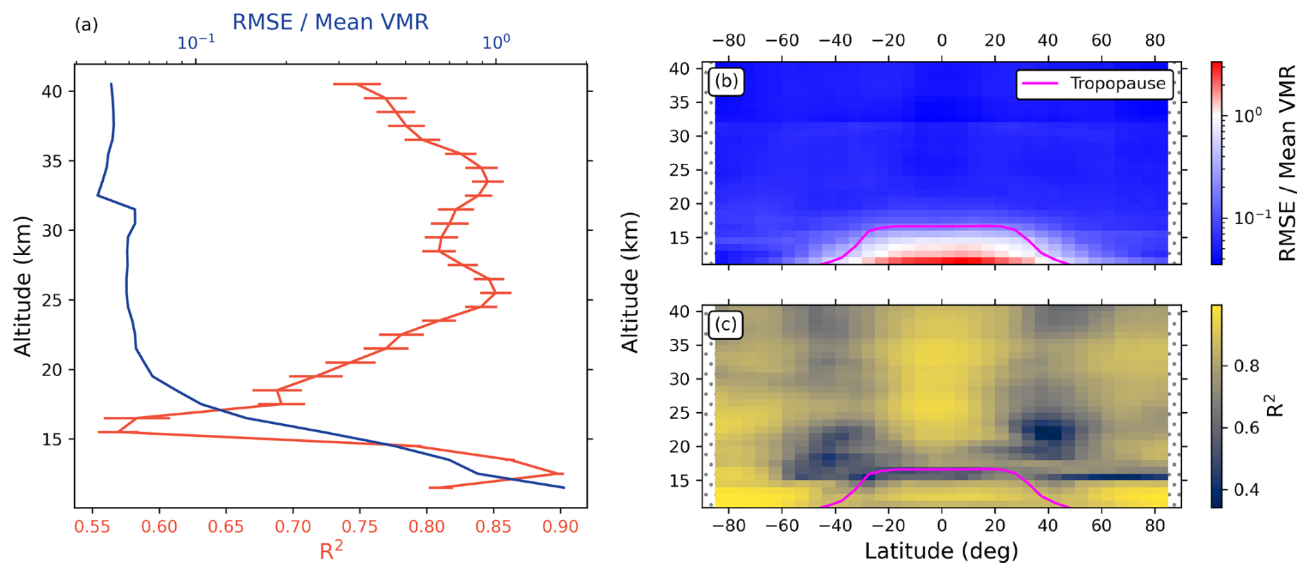
Figure 2 Performance summary for the ensemble of neural networks when applied to the test set. The relative RMSE (RMSE divided by the mean H₂O profile in the training set) is used to better highlight how the errors compare to the average H₂O VMRs at each altitude. Panel (a) shows the performance metrics calculated over the full test set. Error bars denote the standard deviation among the NNs' performances. Panels (b) and (c) show the performance metrics calculated as a function of latitude. Below the tropopause, the RMSE is on the order of or larger than the average H₂O VMR, while in the stratosphere the RMSE is typically < 10 % of the average H₂O VMR.

Figure 2c exhibits local minima in R² in the mid-latitudes. This reduction in R² is a numerical effect associated with how the NN models are trained combined with the variability of MLS water vapor. The equation for R² involves the ratio of the residual sum of squares (RSS) to the total sum of squares (TSS). The combination of the MSE loss function and data normalization procedure optimizes the NN models to make predictions such that the errors (RSS) are relatively evenly distributed (homoscedasticity). TSS, on the other hand, is proportional to the variance of the MLS water vapor values. When MLS water vapor variance is reduced, the R² must also reduce if the agreement between LP and MLS remains constant. These mid-latitude regions are local minima in MLS water vapor variance, and thus they are also local minima in R² given the expected homoscedasticity of the NN models. However, the absolute minimum in water vapor variance occurs in the SH mid-latitudes, while the absolute minimum in R² occurs in the NH mid-latitudes. In the NH, there is an additional effect due to reduced water vapor sensitivity at certain combinations of altitudes, SZA, single scattering angle, aerosol, and H₂O. Based on RTM simulations, the spectral features of water vapor at 930–970 nm shift from reductions in radiances in the SH and tropics to increases in radiances in the NH. At the transition between these regimes, water vapor sensitivity is at its minimum, corresponding to the minimum in R² in the NH mid-latitudes. For more details on this, see Appendix A.

Table 1 summarizes the OMPS LP H₂O product characteristics. The along-track resolution is ∼ 1° for SNPP OMPS LP and ∼ 0.4° for NOAA-21 OMPS LP. Given that the MLS H₂O product has a vertical resolution of 2.8–3.8 km over the pressure range we consider and that the LP vertical field of view is 1.2–1.5 km, the LP H₂O product's vertical resolution may be between 1.2 and 3.8 km. However, more analysis is needed to better estimate the LP H₂O vertical resolution and how it changes as a function of altitude and under different conditions. At present, we conservatively report a vertical resolution ∼ 3.8 km.

Table 1 OMPS LP H₂O product characteristics.

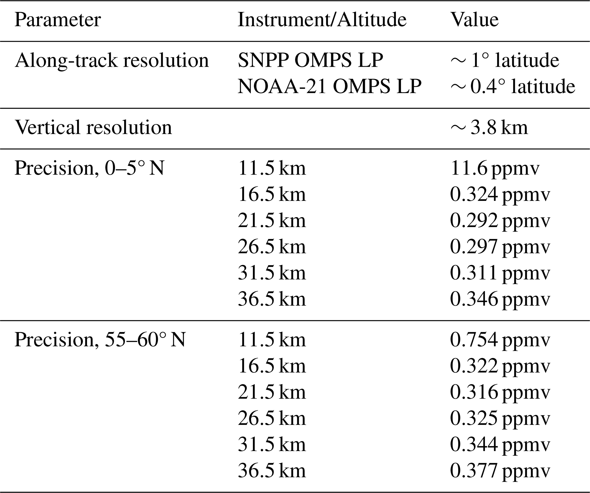
Notes. The reported vertical resolution is a conservative estimate based on the reported vertical resolution for MLS; there is not currently a per-altitude estimate. The reported precision values are the average uncertainties in the specified latitudinal bands.

Figure 3 shows a comparison between the NN, MLS, and LP uncertainties for a co-located event in the tropics in January 2019. The NN uncertainty is smaller than the MLS uncertainty by a factor of ∼ 2.5 in the stratosphere, while in the troposphere the NN uncertainty is larger than the MLS uncertainty by a factor of ∼ 3. Consequently, the combined LP uncertainty is dominated by the NN in the troposphere and by MLS in the stratosphere. We show two cases for this combined LP uncertainty, comprising the lower (uncorrelated) and upper (correlated) bounds for the combined NN-MLS uncertainty. They differ by ∼ 0.1 ppm, which is negligible relative to the volume mixing ratios of typical water vapor profiles. The uncertainties reported within the LP H₂O product are calculated assuming no correlation (see Eq. 1), as the random and systematic errors of MLS are unlikely to be correlated with LP's systematic errors at the wavelengths considered.

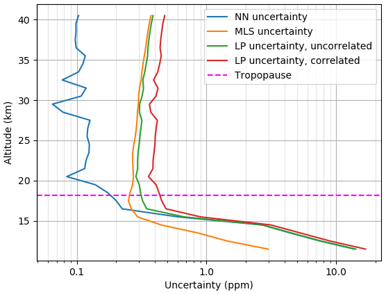
Figure 3 Comparison of uncertainties for a co-located event in the tropics in January 2019. In the troposphere, the NN uncertainty is larger than the corresponding MLS uncertainty by a factor of ∼ 3, while in the stratosphere the MLS uncertainty is larger than the NN uncertainty by a factor of ∼ 2.5. The LP uncertainties are a combination of these NN and MLS uncertainties; the uncorrelated and correlated cases differ by ∼ 0.1 ppm.

The results of our experiments that omit certain years from the training set reveal that some years are more important than others for achieving a well-generalized model. When omitting 2015–2016, we find that the model is generally unaffected and still performs well during those years. However, when omitting 2024, we find that the model begins producing severely inaccurate predictions by March 2024. This behavior is likely explained by the difference between these considered periods: while 2015–2016 were ordinary years in terms of SWV, the continued evolution of elevated SWV from the Hunga eruption into 2024 is atypical and not represented by the data available during 2014–2023. By including a small fraction of 2024 data during training, we find that the model continues performing accurately up to the present time of writing this manuscript. As the stratosphere returns to pre-Hunga conditions, we expect that the NNs will continue producing accurate retrievals of H₂O, but continued comparisons with other instruments designed to measure water vapor, such as ACE-FTS, will be critical to ensuring that accuracy.

Since the input radiances are at wavelengths affected by aerosols, we analyze the model errors as a function of aerosol extinction reported in the OMPS LP aerosol product. We note that a weak anti-correlation exists between the predicted H₂O VMR and the aerosol extinction at 675 nm in the lower stratosphere, though this is a real phenomenon rather than an artifact of our model. Stratospheric aerosol extinction generally peaks immediately above the tropopause and decreases over the few kilometers above it, while stratospheric H₂O VMR typically is at a minimum immediately above the tropopause due to the cold trap and increases over the few kilometers above it. We find that the NNs' percentage error as a function of aerosol extinction at 675 nm is uncorrelated, indicating that the success of our approach is not dependent on aerosol conditions. See Appendix D for additional details.

In general, the differences with respect to MLS are independent of the presence of upper tropospheric clouds identified by the OMPS LP measurements (Chen et al., 2016). However, events affected by polar stratospheric clouds (PSCs) identified by OMPS LP show a median bias around −2 % at most altitudes. When considering the error as a function of distance below the PSC, the median bias can exceed −20 % at 17 km below the PSC, which only occurs for PSCs at ≥ 28.5 km. However, the standard deviation of these errors can be substantial, where it averages around 33 % between 15.5 and 22.5 km, with a maximum of 66 % at 22.5 km. Given this behavior, we recommend that events contaminated by PSCs should not be used for scientific studies; the data product includes quality flags for these events.

4.2 Training on ACE-FTS and SAGE III/ISS data

We also considered training on co-located ACE-FTS and/or SAGE III/ISS data as an alternative to the co-located MLS data set. Results for these experiments were not satisfactory.

When training exclusively on ACE-FTS or SAGE III/ISS data, we find that the resulting NN models do not properly generalize to unseen data, indicating that these data sets are not sufficient to solve this problem. Part of this may be explained by the typically significant measurement time differences between LP and the other instruments; LP measures in the early afternoon, while ACE-FTS and SAGE III/ISS measure at sunrise/sunset, and these times only coincide for select geolocations depending on the time of year. However, the number of co-locations seems to be a more limiting factor. When restricting the MLS data set to similar sizes as the ACE-FTS and SAGE III/ISS data sets, we find that the resulting performance is poor. Given the success when using the MLS-LP data set of ∼ 1 million co-locations but the failure when considering tens of thousands of co-locations, these results emphasize that our methodology relies on a large data set of co-located profiles.

Additionally, when including ACE-FTS and/or SAGE III/ISS data alongside the MLS data, we find significantly degraded performance, regardless of whether or not the ACE-FTS and SAGE III/ISS data were de-biased with respect to MLS. This is likely attributable to the variances between MLS, ACE-FTS, and SAGE III/ISS being on the order of the natural variability of water vapor, which inhibits NN learning.

Despite our negative results when training on ACE-FTS and/or SAGE III/ISS data, we cannot rule out that alternative ML approaches not considered here could utilize ACE-FTS and/or SAGE III/ISS data to derive water vapor profiles from LP radiances.

4.3 Comparisons with satellite measurements

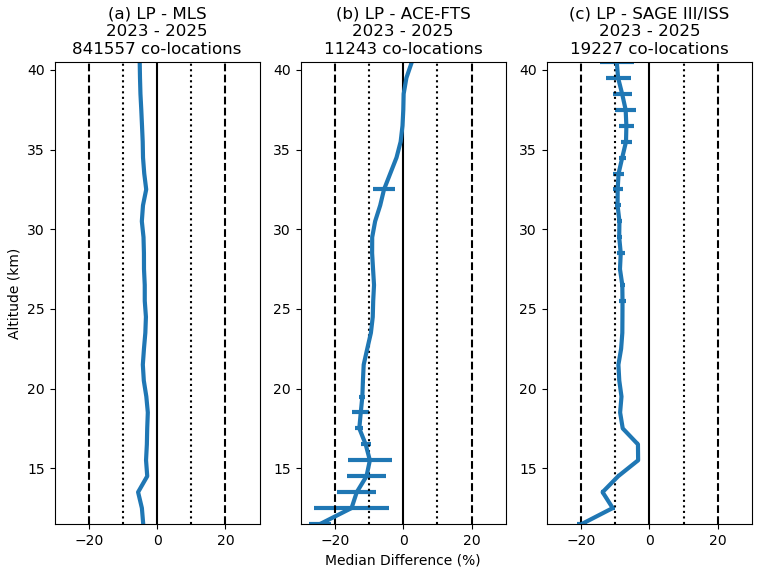
Figure 4 summarizes the global median percent differences between LP stratospheric H₂O profiles and co-located MLS, ACE-FTS, and SAGE III/ISS profiles. For this comparison, we filter all LP tropospheric measurements by using the nearest co-located tropopause altitude reported in the GEOS FP-IT product. The error bars show the standard error of the median, which is generally negligible except at low altitudes for ACE-FTS and at high altitudes for SAGE III/ISS. Where LP detects a cloud, we exclude any measurements at or below the cloud top, though we find that this criterion does not significantly alter the results. Note that for the MLS comparisons we include all co-located data, including those used during training; this choice does not bias the results, as discussed later in Sect. 4.5.

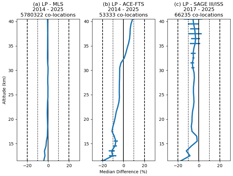
Figure 4 Summary of global median percent differences between the LP stratospheric H₂O profiles and co-located (a) MLS, (b) ACE-FTS, and (c) SAGE III/ISS profiles. Horizontal uncertainty bars indicate the standard error of the median.

Differences with respect to MLS are less than 2 % at all altitudes ≥ 14.5 km, with a maximum difference of 4.1 % at 11.5 km. When considering only 2025 data, the most extreme difference is 7.7 % at 13.5 km, with a typical difference of ∼ 5 % below 22 km and < 2 % above 25 km. Given that we trained on MLS data, this close agreement is expected and shows the model has learned a good approximation to retrieve MLS-like water vapor profiles.

When comparing with ACE-FTS, we find agreement within 10 % except between 11.5 and 13.5 km, where differences can reach up to 19.3 %. In general, the differences increase with altitude from −19.3 % at 11.5 km up to 8.8 % at 40.5 km.

LP's differences with respect to SAGE III/ISS are generally around 6 % or less. Between 11.5 and 13.5 km, differences can reach up to 16.9 %. Given that a similar increase in differences at these altitudes is seen when comparing with both ACE-FTS and SAGE III/ISS but not with MLS, this suggests that either ACE-FTS and SAGE III/ISS are biased high in this regime, or MLS is biased low in this regime and the LP product has inherited this bias.

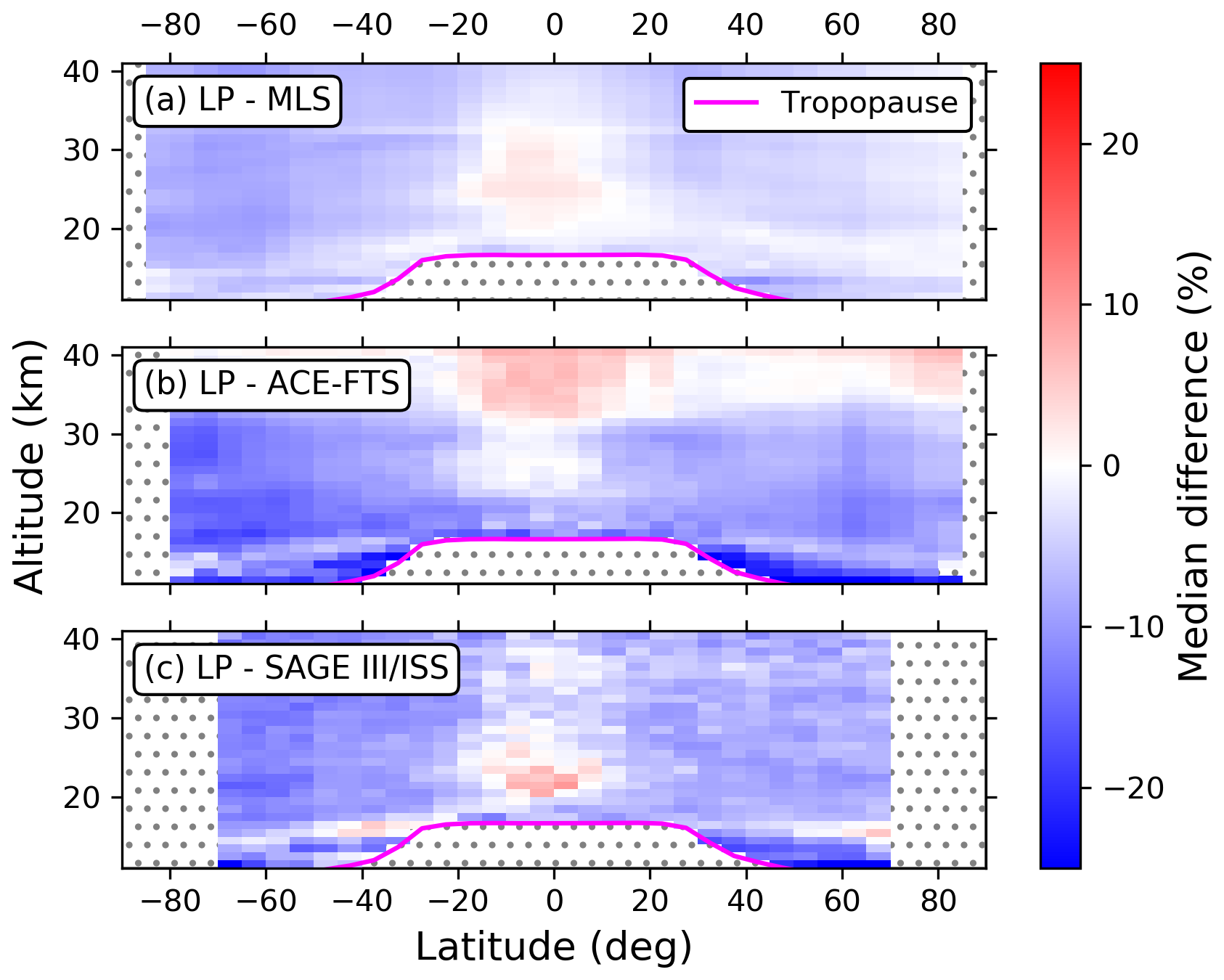
Figures 5 and 6 show the median percent differences and standard error of the median, respectively, in 5° latitudinal bins for the comparisons with MLS, ACE-FTS, and SAGE III/ISS. The results are generally consistent with those shown in Fig. 4. The notable exceptions occur at the lowest altitudes. For the comparisons with MLS, differences can reach up to 8 % between 11.5 and 13.5 km just outside of the tropics. For ACE-FTS, the deviations at these altitudes can exceed 21 %, but notably the standard error of the median is typically ∼ 11 % in this region, suggesting that this low bias may not be as substantial as it appears. However, comparisons with SAGE III/ISS also show this low bias at these altitudes, where the standard error is negligible. Together, this suggests that the LP product has a slight systematic low bias at 11.5–13.5 km just outside the tropics, but at latitudes ≥ 45°, the agreement with MLS suggests the biases when comparing with ACE-FTS and SAGE III/ISS are related to statistical differences between those products and MLS.

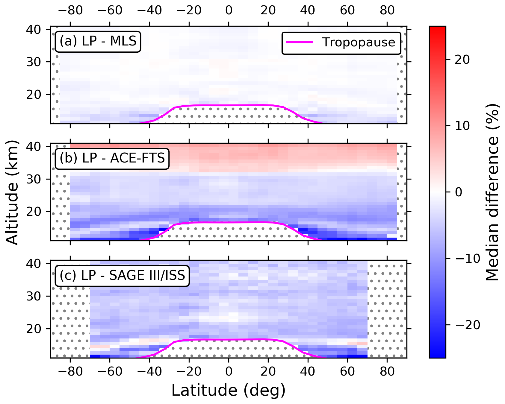
Figure 5 Summary of median percent differences between the LP stratospheric H₂O profiles and co-located (a) MLS, (b) ACE-FTS, and (c) SAGE III/ISS profiles in 5° latitudinal bins. The pink line indicates the median tropopause altitude for a given latitudinal bin. Gray stippling indicates where there are no data, whether due to lack of statistical significance (high latitudes) or due to being in the troposphere (below the tropopause).

Figure 6 Like Fig. 5, but for the standard error of the median.

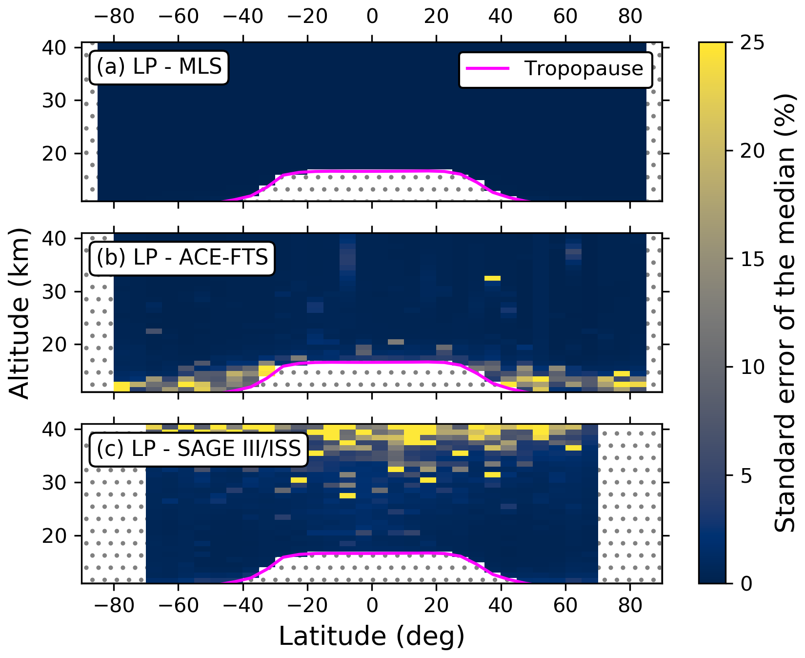
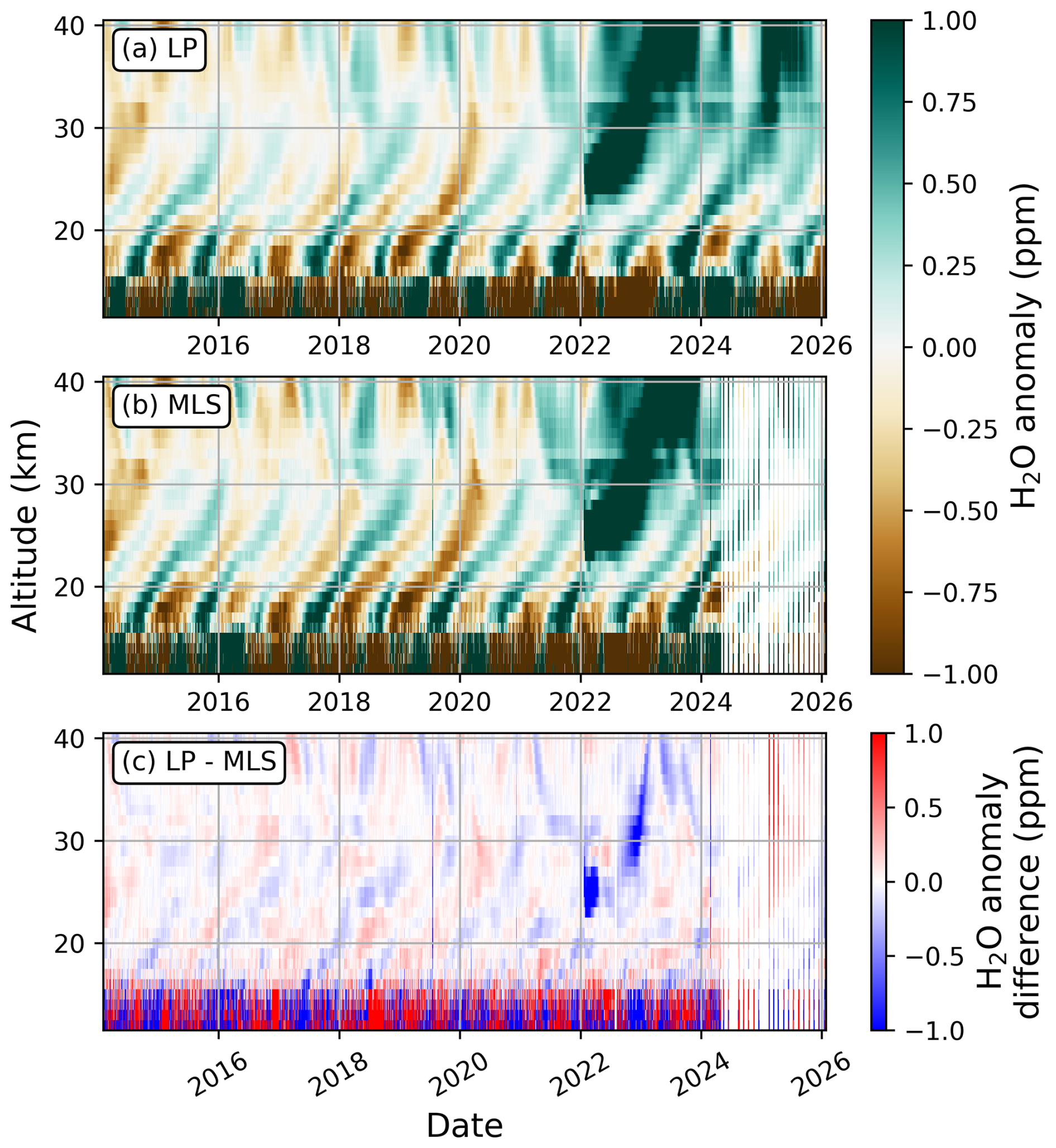
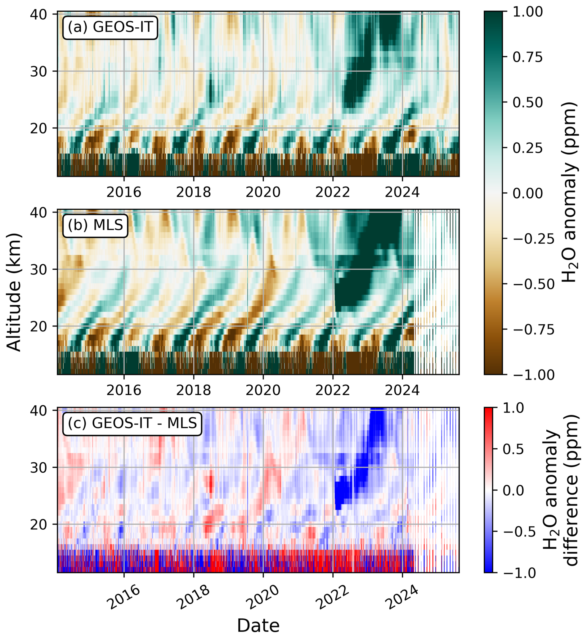
Figure 7 Parts-per-million anomaly in H₂O VMRs for the daily zonal means within 2.5° of the Equator for the (a) OMPS LP and (b) MLS water vapor products. Panel (c) shows the difference between the LP and MLS H₂O anomalies. The anomaly is determined by subtracting the pre-Hunga mean profile from each daily zonal mean profile. Beginning in May 2024, the MLS data become more sparse due to only taking measurements around 6 d each month.

Figure 7 shows the “tape recorder” of alternating positive and negative anomalies in H₂O VMR, primarily attributable to seasonal changes in H₂O. For this plot, we subtract the pre-Hunga mean profile from each daily zonal mean to produce the daily anomaly. Before 2025, the OMPS LP and MLS tape recorders show excellent agreement throughout the stratosphere, with OMPS LP correctly capturing the increase in H₂O due to the Hunga eruption. For ∼ 3 months in early 2025, OMPS LP shows a positive bias > 1.0 ppm above 30 km that is not seen in the corresponding MLS data (Fig. 7c). This bias is likely due to the weak H₂O sensitivity at these altitudes, which inhibits the NNs' ability to reliably infer the H₂O VMR at these altitudes. Since the NNs correctly infer the H₂O at these altitudes before 2025, it suggests that the pre-2025 data were successfully predicted based on the shape of profiles at the lower altitudes that have sensitivity. With an absence of 2025 data in the training set, the NN model relies on profiles from the training data, primarily those influenced by elevated H₂O associated with the Hunga eruption. In 2025, the NNs perform reasonably well below 30 km, suggesting that there is sufficient sensitivity for the determined approximation to remain accurate when applied to unseen data, though there is a slight overestimation (∼ 0.25 ppm) in mid-2025 between 25 and 30 km. We therefore advise that users exercise caution when using the OMPS LP H₂O product above 30 km in the tropics. Additionally, as the excess SWV from Hunga continues to evolve, it is possible that those conditions will be different enough from the training data that the NNs' predictions become inaccurate; we will continue to monitor their performance to ensure the LP NN-based algorithm continues to provide reasonable H₂O profiles.

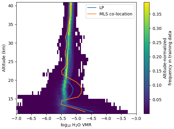
Figure 8 LP and MLS water vapor profiles from 8 January 2020, which feature a lower stratospheric enhancement caused by the Australian wildfires, are plotted over a 2D histogram of the water vapor profiles outside the tropics included in the training data set. Each altitude is normalized such that the probabilities sum to 1. White regions indicate no data. Despite the low frequency of the VMRs of this enhancement in the training data set (< 0.045 %), the ML model successfully identifies this rare situation.

The NNs are largely trained on normal conditions. While Hunga is an anomaly, its impact has lasted years and can be seen globally, and thus the NNs are exposed to various Hunga-affected conditions. Since our data selection process does not consider H₂O concentration or profile states, rare short-lived events are severely undersampled relative to nominal conditions. Despite this, we find that the NN models can still retrieve reasonably accurate profiles for rare cases not seen during training. Figure 8 shows the H₂O profiles retrieved by LP and MLS for an event over the Pacific Ocean on 8 January 2020. This event exhibits a water vapor enhancement in the lower stratosphere due to the intense wildfires in Australia during December 2019–January 2020. Pyrocumulonimbus clouds carried moist, tropospheric air into the lower stratosphere, where it was then transported eastward by winds. Despite that these H₂O concentrations were seen in < 0.045 % of the training data set, the NNs are able to identify this enhancement. The LP and MLS VMRs of this enhancement differ by up to a factor of two, but it is unclear whether this is due to LP underestimating the VMR, MLS overestimating the VMR, a combination of both, or differences in measured air masses.

4.4 Multiple linear regression analysis

In general, the results of our MLR analysis show similar behavior between the LP and MLS products, but the fitted coefficients for the LP data tend to be less than the corresponding MLS coefficients. The main exception to this is the seasonal phase offset, where both products closely agree. Figure 9 shows an example of the fitted coefficients for the seasonal amplitude at 14.5 km. The South Asian monsoon stands out clearly in both panels, though the LP product's fitted amplitudes for this region are around 1 ppm less than the corresponding fits for MLS.

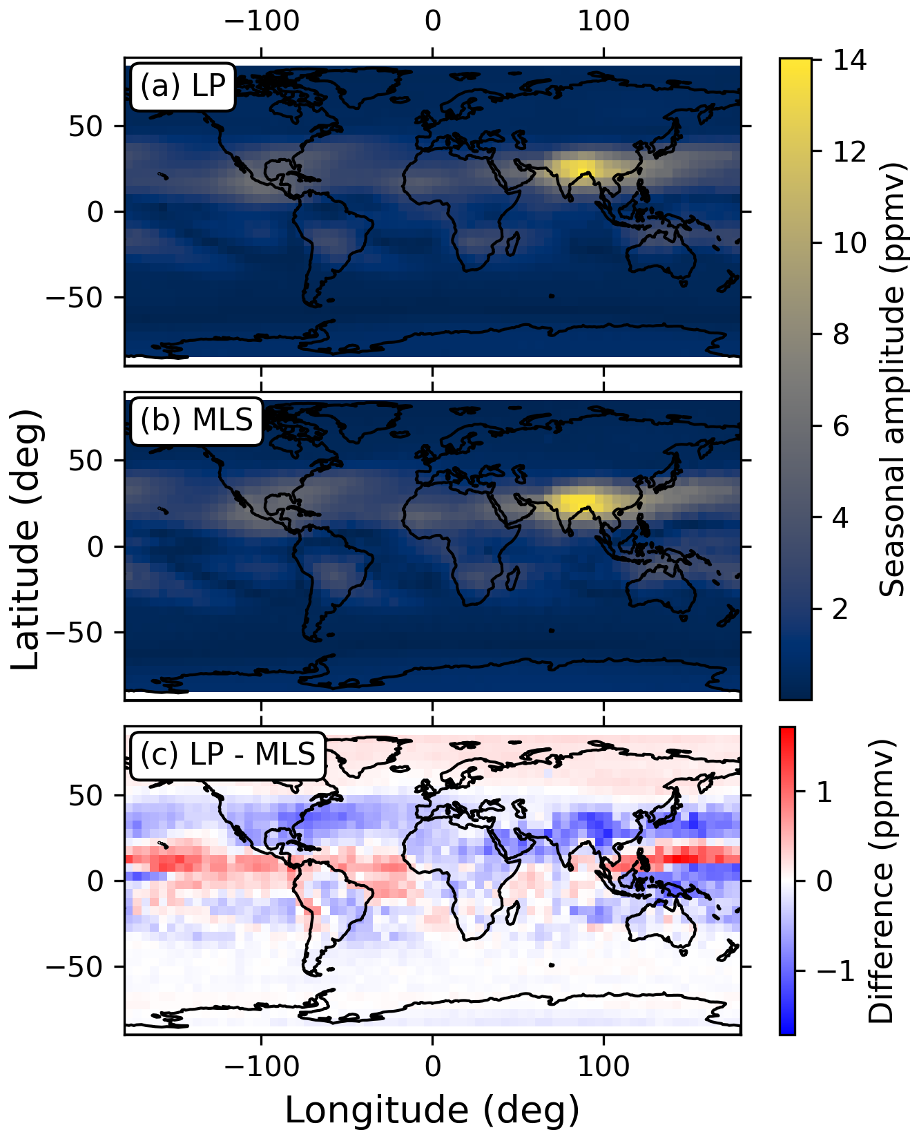
Figure 9 Results for the seasonal amplitude at 14.5 km fitted via MLR for the (a) LP and (b) MLS water vapor products. The large amplitude over South Asia is attributable to the annual monsoon's strong seasonal impact on water vapor. Panel (c) shows the difference between the fitted seasonal amplitude for the LP and MLS products.

Regarding water vapor trends, the LP product generally shows weaker trends in the stratosphere when compared with MLS. In some locations (particularly south and southeast Asia, central Africa, and central America), the LP product shows greater trends in the upper troposphere. Where both products show a trend of increasing H₂O, LP tends to show a lesser trend than MLS (Fig. 10).

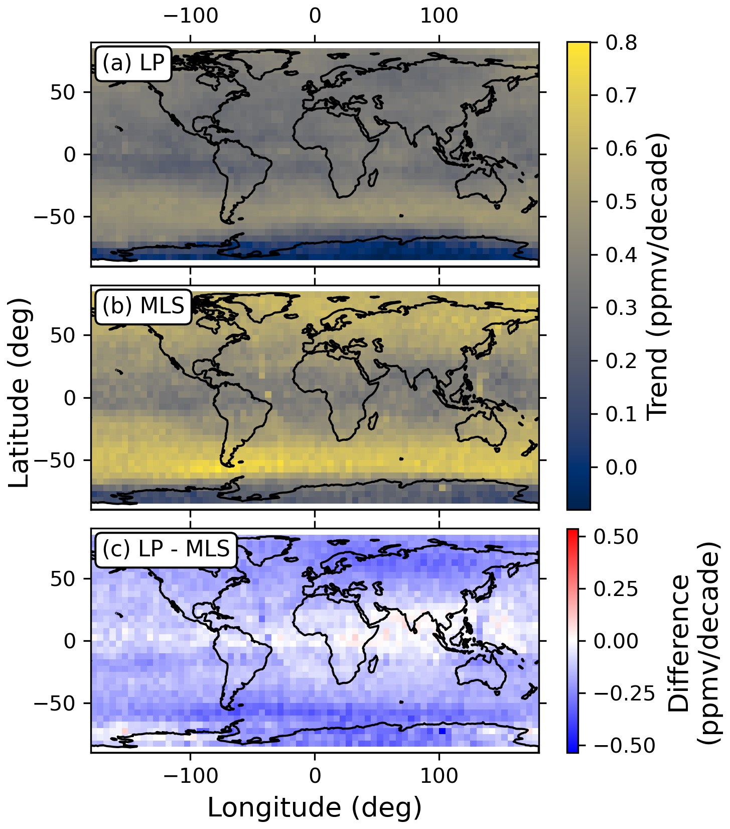
Figure 10 Results for the linear trend in H₂O at 18.5 km fitted via MLR for the (a) LP and (b) MLS water vapor products. In general, LP shows a weaker trend of increasing H₂O than MLS.

4.5 Comparisons with M2-SCREAM

Figure 11 compares the OMPS LP and M2-SCREAM H₂O products for the year 2021. Note that M2-SCREAM assimilates MLS v4.2, which is biased high for water vapor, while LP is trained on MLS v5, resulting in a persistent ∼ 0.5 ppmv bias between the products. Days in which data were (Fig. 11a) or were not (Fig. 11b) included during training are shown separately but look almost identical, highlighting that the NNs' predictions are equally accurate whether or not they saw data from that day during training. Additionally, the standard deviation of the differences between OMPS LP and M2-SCREAM are consistently less than the standard deviation among OMPS LP or M2-SCREAM profiles, indicating that the OMPS LP product is more accurate than the natural variability of H₂O. Overall, our results suggest that the NN predictions are in good agreement with M2-SCREAM for data not seen during training.

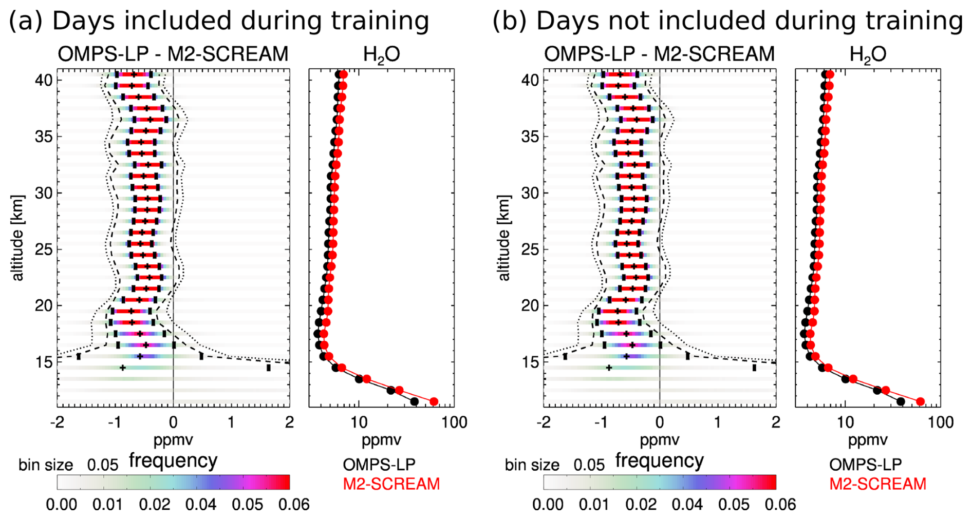
Figure 11 Comparison between OMPS LP and M2-SCREAM for days in 2021 where (a) some data were included during training and (b) no data were included during training. Note that for days in which data were included during training, only a small percentage (1 %–4 %) of data on those days were used in the training data set. For each panel, the left subpanel shows the probability density function of the differences between OMPS LP and M2-SCREAM as horizontal colored bars, one standard deviation of the differences as the vertical marks, the mean difference as plus signs, the mean difference ± the standard deviation of OMPS LP H₂O as dashed lines, and the mean difference ± the standard deviation of M2-SCREAM as dotted lines. The right subpanel shows the mean H₂O profile for each product. Panels (a) and (b) look nearly identical, indicating that the model is retrieving H₂O from the information content embedded in LP radiances rather than blindly memorizing the training data. The ∼ 0.5 ppmv offset between the products is due to differences in the MLS version used by each product.

4.6 Comparisons with balloon-borne measurements

Figure 12 shows the median differences between satellite instruments (MLS, SAGE III/ISS, ACE-FTS, and OMPS LP) and the frost point hygrometer soundings from the six stations considered (see Sect. 3.3). The LP product agrees with the frost point measurements within 0.3 ppmv and within 10 % between 16.5 and 27.5 km; this is in close agreement with the MLS results, which is expected given that we trained on MLS data. The only notable difference in agreement between MLS and LP is that the LP product shows a slightly reduced bias between 16.5 and 21.5 km. Like in Davis et al. (2021), we find that the satellite instruments show a dry bias in the upper troposphere compared to the frost point measurements, which may be due to spatiotemporal variability between the co-located measurements and/or reduced data quality in this regime.

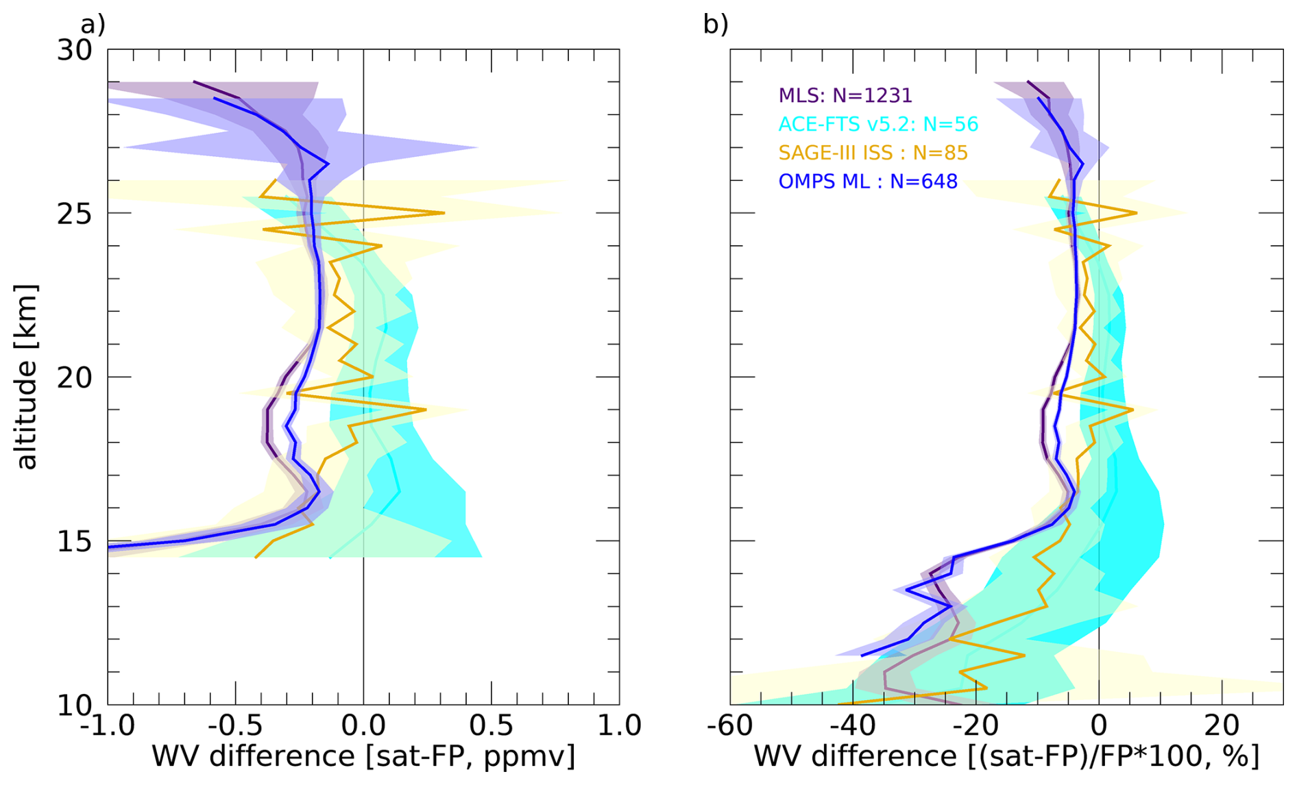
Figure 12 Comparisons between satellite instruments and frost point balloon measurements. Panel (a) shows the median difference in ppmv limited to altitudes where the mean water vapor is < 10 ppmv, and panel (b) shows the median percent difference. In both panels, the shaded regions show the median ± 2 standard errors of the mean.

4.7 Application to NOAA-21 OMPS LP

Paralleling the SNPP comparisons in Sect. 4.3, Figs. 13 and 14 show respectively the global median percent differences and the 5° zonal median percent differences between NOAA-21 OMPS LP and MLS, ACE-FTS, and SAGE III/ISS. For global comparisons, NOAA-21 OMPS LP shows a persistent ∼ 5 % offset with respect to the corresponding SNPP comparisons at all altitudes. A similar low bias is seen in the NOAA-21 OMPS LP aerosol data, suggesting that this bias is attributable to differences in radiances between OMPS LP on SNPP and NOAA-21. Given our methodology, it is unclear whether the NNs have learned to implicitly account for a bias in the SNPP radiances or if the problem is related to the calibration of NOAA-21 radiances. However, this bias is not strictly a −5 % shift for all conditions; the zonal comparisons show that the tropics exhibit a positive bias not seen in the corresponding SNPP comparisons. Further investigation is necessary to understand the cause of these biases. If the origin of these biases is not able to be determined, they could be addressed via a soft calibration approach.

Figure 13 Like Fig. 4, but for NOAA-21 OMPS LP.

Figure 14 Like Fig. 5, but for NOAA-21 OMPS LP.

5 Conclusions

We presented a water vapor retrieval product derived from SNPP OMPS LP measurements via a neural network (NN) trained on co-located MLS version 5 water vapor profiles. In general, the LP H₂O product is consistent with other water vapor products considered here. We find that our method typically agrees with MLS within 5 % at all altitudes considered. The results of our multiple linear regression analysis show good correspondence between LP and MLS for seasonal water vapor variations, including for the south Asian monsoon. LP's tape recorder in the tropics also shows close agreement with MLS, capturing both the alternating positive and negative seasonal anomalies as well as the large water vapor injection from the Hunga eruption. Agreement with SAGE III/ISS version 6 and ACE-FTS version 5.3 water vapor profiles is typically within 10 % above 15 km and within 20 % below 15 km. When compared with frost point balloon measurements, OMPS LP generally agrees within 10 % in the stratosphere, closely mirroring comparisons between those frost point measurements and MLS. Comparisons with the M2-SCREAM reanalysis product show similar behavior between days included in training and days omitted from training, indicating that our method is retrieving H₂O from the LP radiances rather than memorizing the training data. Overall, we find that the LP product generally performs comparably to MLS over the 11.5–40.5 km altitude range considered, enabling the continuation of the MLS water vapor record for these altitudes. The exception is in the tropics above 30 km, where a period in 2025 shows larger errors relative to MLS than those seen during the 2014–2024 training period; we advise that users exercise caution when using LP H₂O data in this regime.

When applying the same methodology but using SAGE III/ISS and/or ACE-FTS data for training, we find significantly reduced performance. We similarly find poor performance when limiting the MLS-LP data set to the same size as the SAGE III/ISS and ACE-FTS data sets, which suggests that the success of our approach relies on a large training data set of co-located profiles. When including SAGE III/ISS and/or ACE-FTS data alongside MLS data, we also find poor performance, regardless of whether or not the SAGE III/ISS and ACE-FTS data are bias corrected to have a 0 % median difference with MLS at all altitudes. This suggests that the variances between the three satellite data products inhibit NN learning.

Despite insufficient co-located data to train a well generalized model specific for NOAA-21 OMPS LP, we find that the SNPP-trained NN is applicable to NOAA-21 OMPS LP measurements without retraining. For NOAA-21 data, we find a persistent negative bias of ∼ 5 % under most conditions when compared with the corresponding SNPP results; this pattern is also seen in comparisons between the SNPP and NOAA-21 OMPS LP aerosol products, suggesting that it is due to differences in the radiances rather than poor generalization of the SNPP-trained NN. However, the source of this bias is unclear at the time of writing; future work should explore approaches to identify the origin of this bias, characterize it, and correct it, if possible. Assuming that the NN model continues performing well over the coming years, our results suggest that this SNPP-trained model will be applicable to OMPS LP onboard JPSS-4 and 3, which are planned to launch in 2027 and 2032, respectively, thereby extending the MLS water vapor record into the 2030s, albeit at a reduced altitude range. Continued satellite and balloon-borne measurements from instruments with physics-based stratospheric H₂O products, such as ACE-FTS, SAGE III/ISS, and frost point hygrometer soundings, will be integral to ensuring that our NN-based retrievals continue to perform well in the coming years.

Appendix A: Additional details on OMPS LP sensitivity to H₂O

To better understand OMPS LP's sensitivity to H₂O, we use the GSLS RTM (Herman et al., 1994; Loughman et al., 2004, 2005, 2015) to simulate viewing conditions and atmospheric states measured by OMPS LP. Results can be grouped into two regimes, based on the impact of aerosols: the southern latitudes and tropics, and the northern latitudes. In the southern latitudes and tropics, aerosol scattering does not significantly impact the H₂O signal. In the northern latitudes, LP's viewing conditions measure forward scattering from aerosols, resulting in significant changes in radiances that reduce the relative strength of the H₂O signal.

Figures A1 and A2 show the RTM simulations and OMPS LP measurements, respectively, for an event in the tropics on 3 May 2019. A decrease in radiances attributable to H₂O absorption can be seen between 930 and 970 nm. The RTM simulations also show weak absorption around 724 and 824 nm, but the LP measurements do not have any obvious absorption features there. It is important to highlight that the RTM contains a number of simplifying assumptions that are not representative of reality (e.g., it assumes a simple reflective surface at the bottom of the atmosphere and ignores water vapor absorption within clouds) and therefore may be missing some important contributions in this regime necessary to model real measurements.

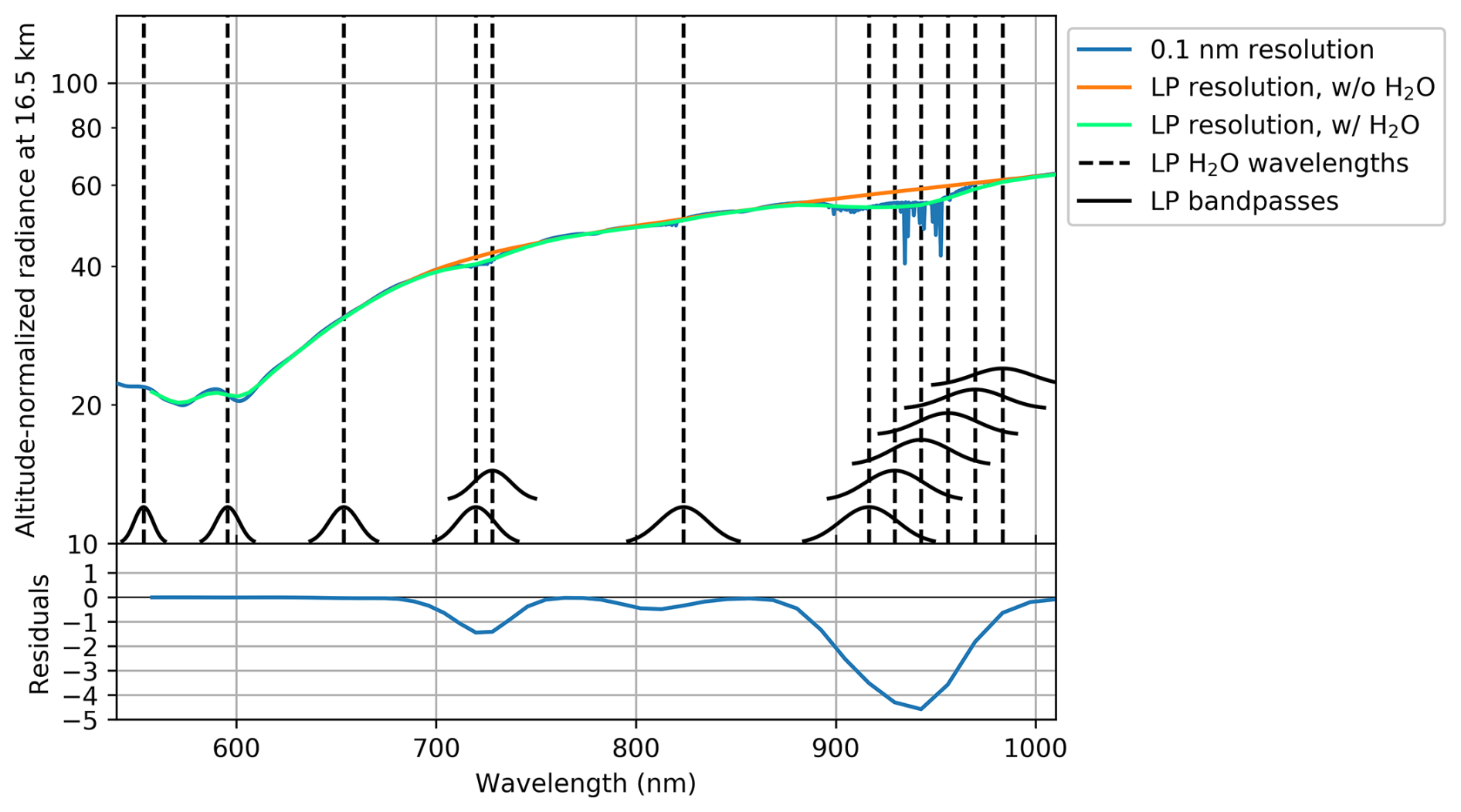
Figure A1 Radiative transfer simulations with and without H₂O based on a measurement by OMPS LP on 3 May 2019 at 5.4° N latitude, 106.7° E longitude, where the solar zenith angle is 23.2° and the single scattering angle is 103.6°. Temperature and pressure profiles are from GEOS IT; O₃, surface reflectivity, and the aerosol extinction profile at 675 nm (extrapolated to other wavelengths assuming a gamma-function size distribution) are from the OMPS LP ozone retrieval algorithm; and the H₂O profile is from a co-located MLS measurement. Radiances are altitude normalized at 40.5 km. Black dashed vertical lines mark LP channels used in the ML model for the H₂O retrievals. The LP bandpasses are shown as black curves, which are vertically shifted to avoid overlaps. Original RTM simulations with water vapor absorption are performed at a 0.1 nm spectral resolution (blue curve). Simulated radiances convolved with LP bandpasses are shown in green. Convolved radiances simulated without accounting for water vapor absorption are shown in orange. The lower panel shows the differences between convolved radiances simulated with and without water vapor (differences between orange and green lines), highlighting spectral regions where water vapor absorption is expected.

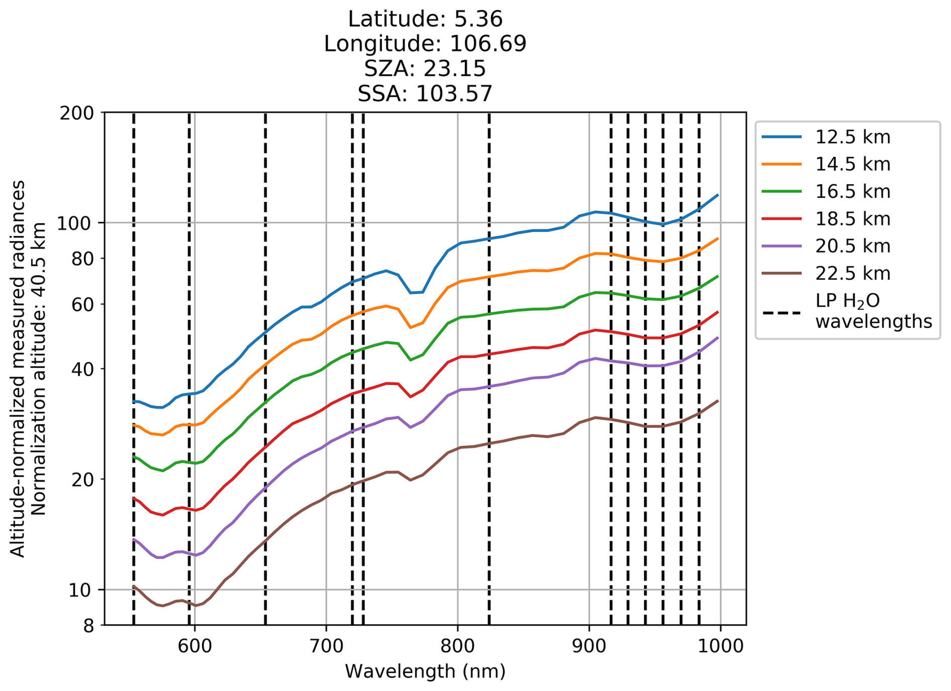
Figure A2 Altitude-normalized radiances measured by OMPS LP for the event modeled in Fig. A1. At these altitudes, including in the lower stratosphere, a small decrease in radiances is observed around 930–970 nm, which we believe is attributed to water vapor absorption. However, the measured radiances do not show reduction around 720 and 824 nm as predicted by the RTM simulations, possibly due to the RTM's simplifying assumptions.

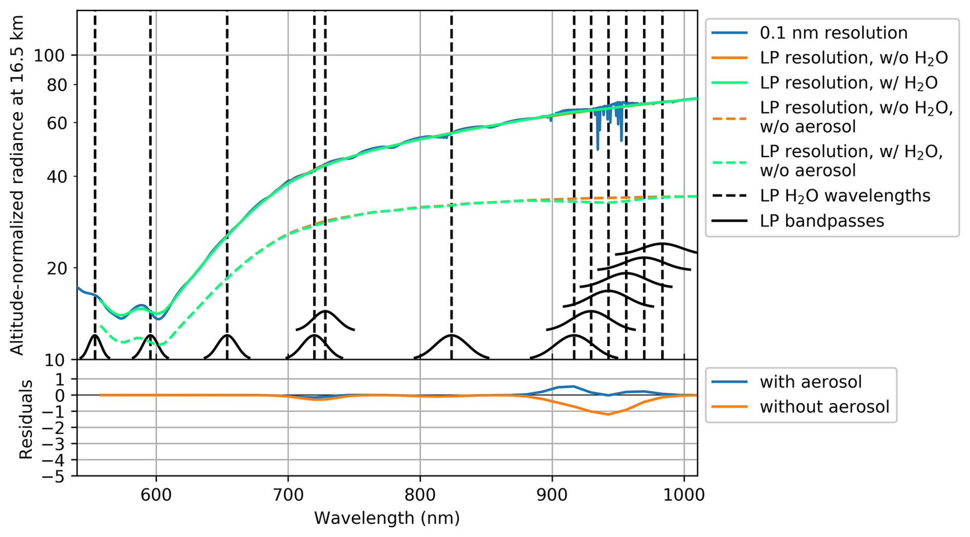
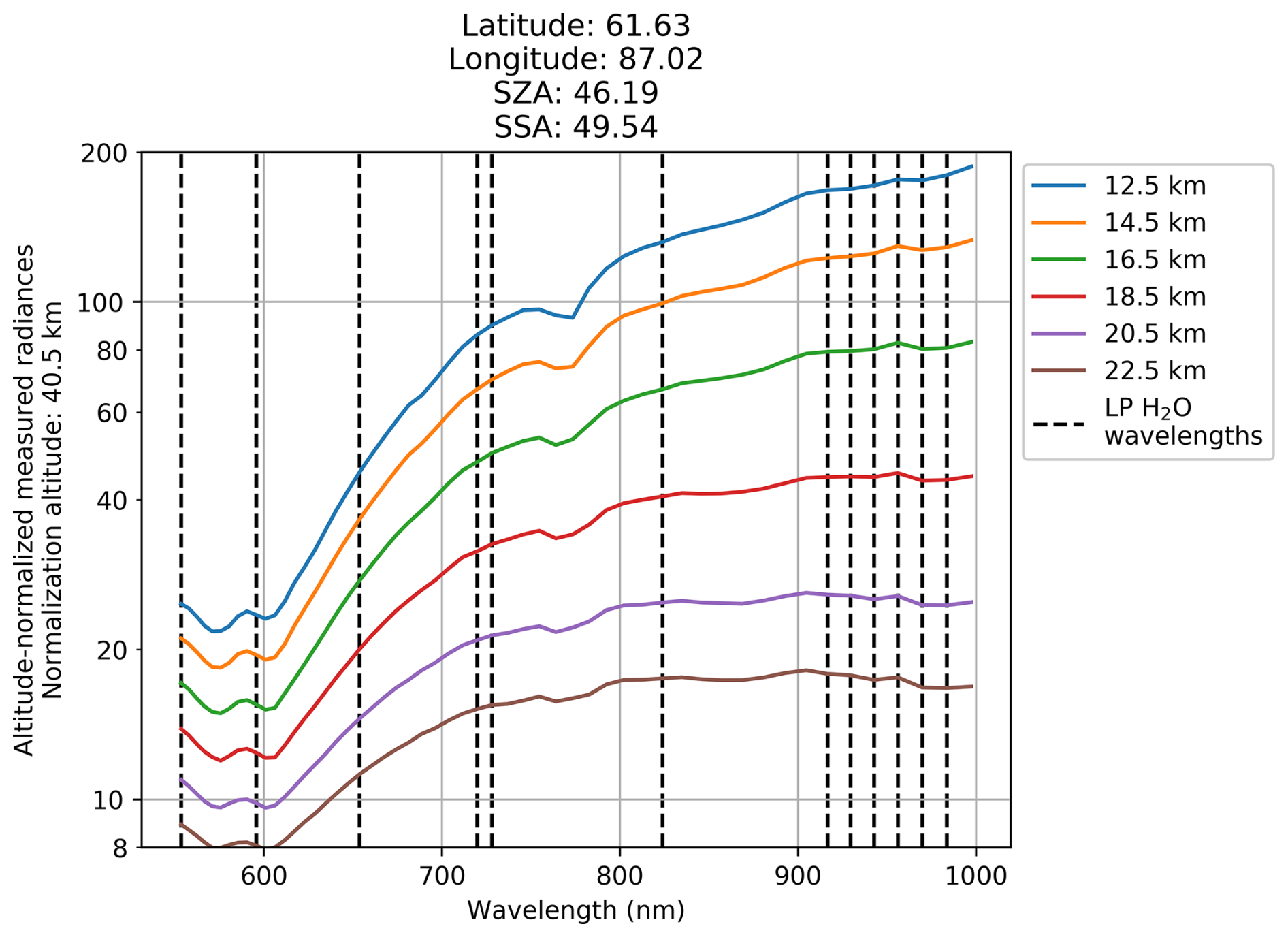
Figure A3 Like Fig. A1, but for a measurement at 61.6° N latitude, 87.0° E longitude, solar zenith angle of 46.2°, and a single scattering angle of 49.5°. Simulations without aerosol are shown as dashed orange and green lines. Unlike in Fig. A1, the lower panel here shows almost no differences between the simulations with and without H₂O in 930–970 nm spectral range, and even indicate a small increase in radiances simulated with H₂O compared with the simulation without H₂O. When omitting aerosol, radiances decrease due to H₂O absorption, confirming the increase in radiances for these viewing conditions is due to aerosol.

In the northern hemisphere, the H₂O signal become less clear. The interaction between aerosol scattering and H₂O causes the H₂O signal to weaken under these conditions, leading to no notable changes or even a small increase in radiances, rather than decrease as seen in the tropics and southern latitudes. Figure A3 shows RTM simulations for the viewing conditions and atmospheric state of a measurement by  OMPS LP  in the northern mid-latitudes on  3 May 2019. The simulation with H₂O shows no water vapor absorption but rather shows a small increase in radiances. When neglecting aerosols, this setup produces a water vapor absorption signature between 930 and 970 nm as expected. Figure A4 shows the OMPS LP measurement for those conditions; there are no obvious spectral features attributable to H₂O, though the small positive bump at 956 nm may be related. Given the RTM results, there must be some transition region where the H₂O absorption feature vanishes before the radiances begin to increase as seen in Fig. A3. That transition region likely occurs for specific combinations of SZA, single scattering angle, aerosol, and H₂O. Given the larger than expected reduction in R² around 40° N in Fig. 2, we believe that feature is in part explained by reduced H₂O sensitivity in this transition region. Measured radiances at higher latitudes begin to show a negative spectral slope in the 930–970 nm range, rather than monotonically increasing as would be expected under conditions with a strong aerosol signal, which we believe may be indicative of H₂O.

Figure A4 Like Fig. A2, but for the event simulated in Fig. A3. Unlike in Fig. A2, there are no obvious spectral features attributable to H₂O in the 930–970 nm spectral band.

Rozanov et al. (2011) found that doubling tropospheric H₂O causes significantly larger changes to visible and near-infrared stratospheric radiances than doubling stratospheric H₂O, except in the 1353–1410 nm range where stratospheric perturbations result in larger changes to stratospheric radiances. We selected an OMPS LP measurement from 21 September 2015 to carry out a similar test using the GSLS RTM. The tropopause height and the temperature and pressure profiles are from GEOS-IT, the O₃ profile is from climatology, the surface reflectivity is set to 0.28, and the H₂O profile is from a co-located MLS measurement. For these tests, we neglect aerosols. Figure A5 shows the change in convolved radiances at various OMPS LP wavelengths when doubling H₂O at each altitude (a) in the stratosphere and (b) in the troposphere. Consistent with Rozanov et al. (2011), we find that doubling tropospheric H₂O has a more significant impact on stratospheric radiances than doubling stratospheric H₂O. However, when applying altitude normalization, we find the reverse. Figure A6 shows the change in convolved radiances when applying altitude normalization at 40.5 km, demonstrating that doubling stratospheric H₂O has a more significant impact on altitude-normalized stratospheric radiances than doubling tropospheric H₂O. Whether altitude normalization is applied or not, Figs. A5 and A6 show that the change in radiances is < 3 % when doubling H₂O concentrations for these conditions. Despite that high surface reflectivities boost the impact of tropospheric perturbations and reduce the impact of stratospheric perturbations, it is not significant enough to alter these conclusions. However, given the RTM limitations mentioned above, it is possible that altitude normalization of real measurements does not cancel out contributions from tropospheric H₂O as much as suggested by these simulations.

Based on these analyses of simulated and measured radiances, we believe that the ML model derives water vapor from the spectral dependence of measured radiances and is able to distinguish different conditions by being exposed to a large range of cases during the training. Given the ML model’s agreement with MLS, ACE-FTS, and SAGE III/ISS when applied to LP measurements in 2025 and 2026, the model can infer H₂O at northern high latitudes, because otherwise a lack of information content would manifest as reduced performance in NH regions compared to other regions, which are not seen in our validation results. In an experiment where we added single scattering angle as additional input parameter (note that single scattering angle is consistently different between southern and northern hemispheres for the LP viewing geometry and can serve as a proxy for aerosol contamination), we found no change in results. This test, coupled with the tests in Appendix B, confirms that the model relies on the spectral signature of measured radiances to infer the information about the water vapor concentration under different conditions.

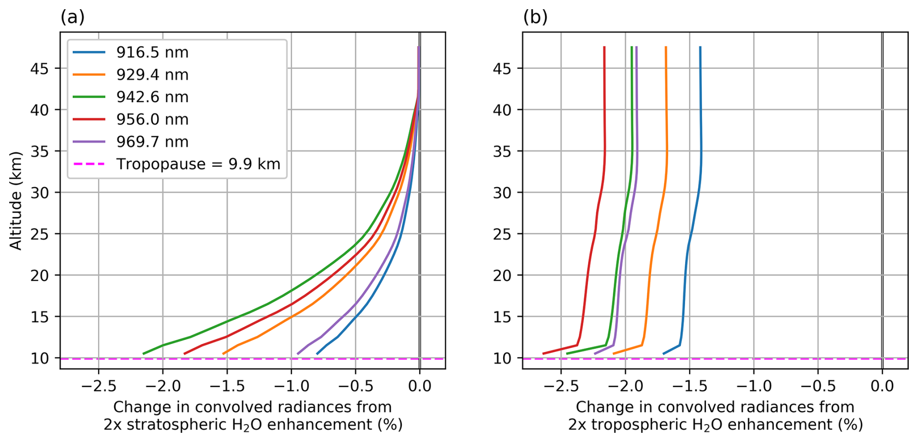
Figure A5 Change in convolved radiances at LP's resolution when doubling H₂O at each altitude (a) in the stratosphere and (b) in the troposphere. Tropospheric perturbations in H₂O have a larger impact than stratospheric perturbations.

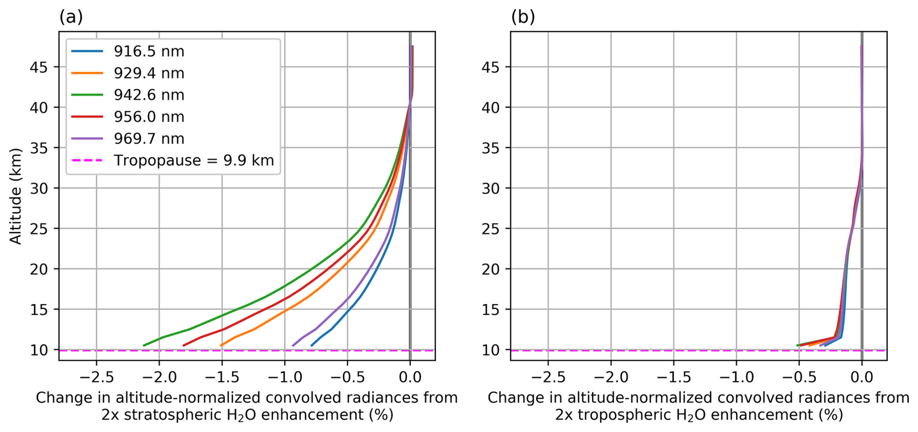
Figure A6 Like Fig. A5, but for convolved radiances altitude-normalized at 40.5 km. Altitude normalization cancels out much of the diffuse light coming from the surface and troposphere, leading to stratospheric perturbations having a larger impact than tropospheric perturbations on stratospheric radiances.

Appendix B: Investigation of relative importance of neural network input parameters

The NNs presented in the manuscript utilize a combination of LP radiances and solar zenith angles as well as GEOS-IT data for temperatures and pressures. To roughly assess the relative importance of these inputs, we conducted experiments where NNs were trained on (1) only the meteorological GEOS-IT data, (2) only the LP radiances, and (3) using pressure/temperature climatology in place of GEOS-IT data.

Figure B1 shows the NN ensemble's RMSE and R² values for the model presented in the manuscript alongside those performance metrics for NNs trained on (1) only the GEOS-IT meteorological data and (2) only LP radiances. The reduced performance of the NN trained on only GEOS-IT data indicates that the LP radiances enable the determination of a better solution for retrieving SWV. This performance difference can also be seen in Fig. B2, which shows the taperecorder plot for the NN trained only on the GEOS-IT data. Notably, the GEOS-IT-only NN model features positive anomaly artifacts (especially in mid 2018), misses the SWV enhancement in January 2022 attributable to the Hunga eruption, and consistently shows larger deviations from MLS in 2025 than those seen in Fig. 7. In contrast, the NN trained on only LP radiances and climatological meteorological data result in almost the same performance as the NN ensemble presented in the main text of the manuscript. Given these results, we conclude that the LP radiance data are the primary source of information content for this problem.

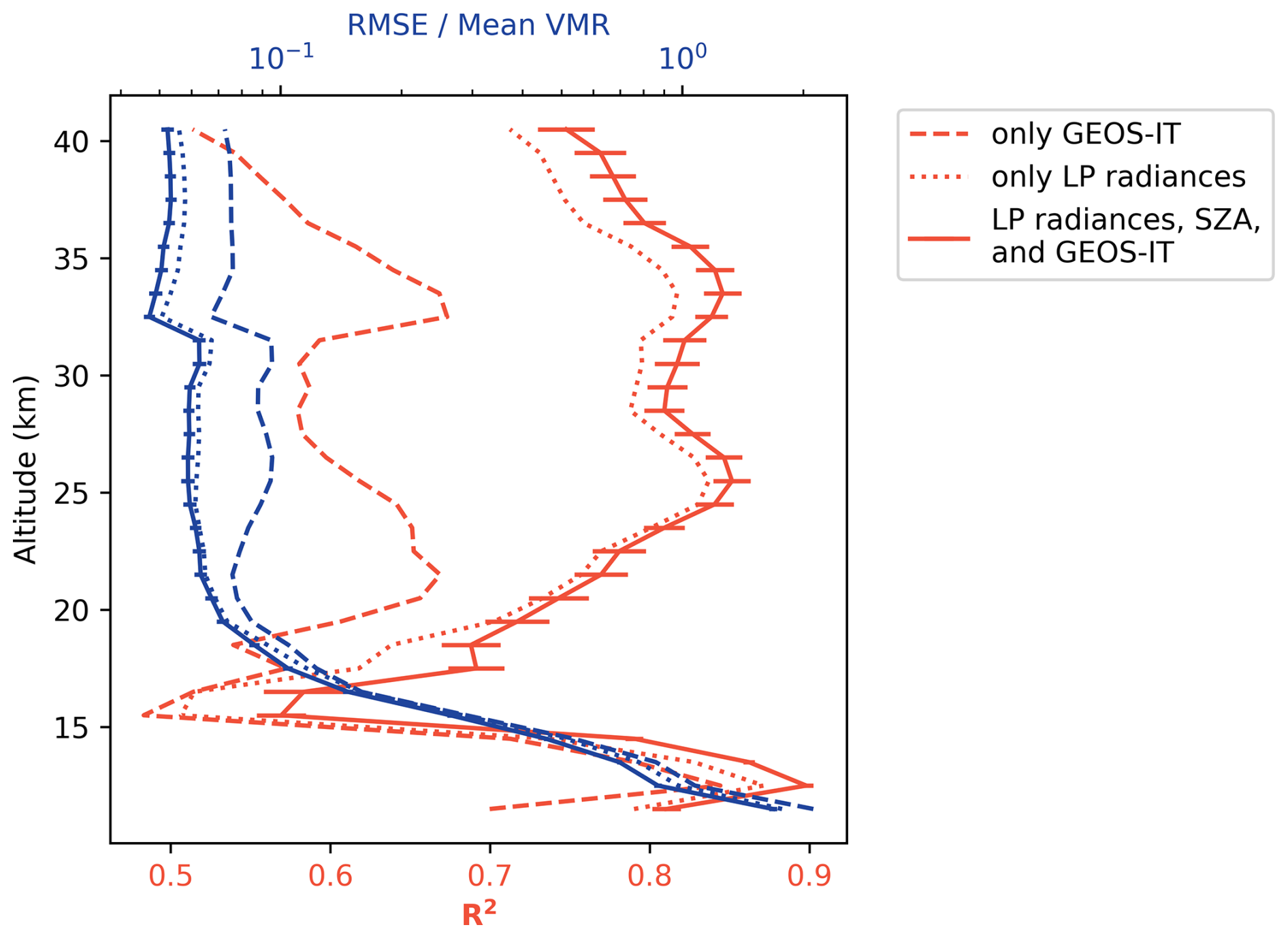
Figure B1 Like Fig. 2, but also including results for NNs trained on (1) only GEOS-IT meteorology and (2) only LP radiances. The performance gap between the model trained on only GEOS-IT data and those trained with LP radiances indicates that the LP radiances offer additional information that enables a more accurate model.

Figure B2 Like Fig. 7, but for the NN trained on only the meteorological GEOS-IT data. The absence of LP radiance and solar zenith angle data results in reduced performance.

Appendix C: Neural network optimization, architecture, and training

To optimize the neural network architecture for this problem, we performed a Bayesian hyperparameter optimization over the number and types of layers, number of nodes per layer, and activation functions. We considered fully connected NNs, convolutional NNs, and architectures that utilize both fully connected and convolutional layers. In addition to standard fully connected layers, we also considered Concrete Dropout layers (Gal et al., 2017), which include a trainable parameter for the layer's dropout rate. For convolutional architectures, we considered architectures with and without pooling layers.

The selected architecture is similar to the landmark AlexNet architecture (Krizhevsky et al., 2012), with hidden layers and activation functions consisting of Conv2D(32)–ReLU–MaxPool2D–Conv2D(64)–ReLU–MaxPool2D–CD(256)–ReLU–CD(256)–ReLU, where Conv2D(m) indicates a two-dimensional convolutional layer with m feature maps using a kernel size of 5, ReLU indicates the rectified linear unit activation function, MaxPool2D indicates a two-dimensional pooling layer that selects the maximum value within a 2 × 2 window, and CD(n) indicates a Concrete Dropout layer with n nodes. This is followed by a fully-connected output layer of 30 nodes, corresponding to the H₂O VMR at the 30 altitudes spanning 11.5–40.5 km. Note that other architectures performed similarly to the selected architecture; we found that the training data set played a more significant role in model performance.

We optimized the learning rate policy according to the method described by Himes et al. (2025b) and trained each NN using the mean-squared-error loss over the validation set until early stopping engaged after a patience of 60 epochs. On average, models trained for 638 epochs, which required an average of almost 7 h to train using an Nvidia V100 graphics processing unit.

On our processing system, running our retrieval algorithm using the central processing unit requires around 12 and 16 s to process one SNPP and NOAA-21 orbit, respectively; specialized graphics processing units would reduce this runtime.

Appendix D: Evaluation of sensitivity to aerosols

The LP wavelengths used in this study are affected by aerosols. However, as discussed in Sect. 4.1, the NN model errors are generally uncorrelated with aerosol extinction. Figure D1 shows a 2-D histogram of LP-MLS differences vs. aerosol extinction at 675 nm. The vast majority of the probability density is found clustered around a difference of ∼ 0 %. At the largest extinctions (> 0.01), there appears to be a slight negative bias, but this is generally related to the negative bias associated with PSCs discussed in Sect. 4.1. Figure D2 shows a time series of mean orbital LP-MLS differences, with three major eruptions over this time period marked for reference. The LP-MLS differences do not feature any notable deviations in the time following these eruptions, suggesting that variations in aerosol loading do not negatively impact the model performance.

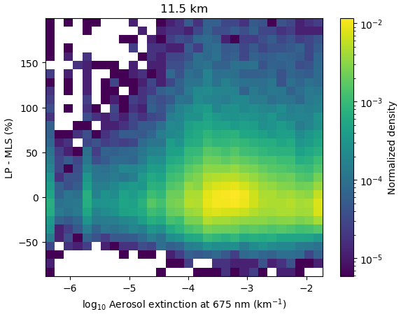
Figure D1 Histogram of the LP-MLS percent differences vs. OMPS LP aerosol extinction at 675 nm at 11.5 km. Errors are clustered around 0 %, indicating aerosols do not significantly impact model performance.

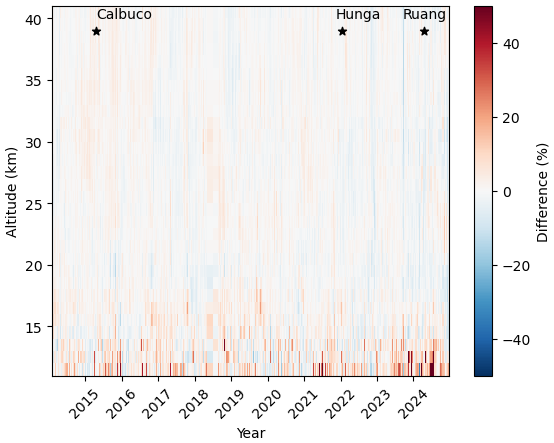
Figure D2 Time series plot of the average percentage difference between LP-MLS co-locations per LP orbit. Three major eruptions are denoted on the plot for context. Errors appear unrelated to those major eruptions.