Atmospheric deposition of microplastics: a sampling and analytical method including the associated measurement uncertainties

Microplastics (MPs) are environmental contaminants of global concern, and the atmosphere may play an important role in their environmental distribution. In this study, we developed a tailored analytical chain – including sample collection, processing, and analysis based on optical microscopy and focal plane array μ-Fourier transform infrared spectroscopy (FPA-μ-FTIR) – to quantify 20–215 µm MPs (excluding tire wear particles) in wet and dry atmospheric deposition samples. We present a novel sampling setup to collect particulate wet deposition, which consists of an on-site precipitation filtration device. Validation of the sampling setup via spike-recovery experiments using surrogate standards resulted in average recoveries of approximately 90 %, suggesting limited MP losses. Additionally, we developed a custom software platform that combines the results from optical microscopy and chemical imaging obtained through FPA-μ-FTIR. Furthermore, an assessment of the total measurement uncertainty was made by addressing each step of the analytical chain individually. The resulting total expanded uncertainty was approximately 90 % for determining MP numbers in a single wet or dry deposition sample. The conversion of MP numbers and associated size information into MP mass was estimated to generate an additional systematic error of 50 %. Based on analyses of blanks, the critical level and the limit of detection, number-based thresholds for minimizing false positives and false negatives, were 29 and 58 MPs per analyzed subsample, respectively. The analytical chain was applied to quantify the MP content in wet and dry atmospheric deposition samples collected at a suburban site in Switzerland. The principles and methodology used in this study to calculate the uncertainties, recoveries and limits of detection are transferrable to other analytical methods intended for MP analysis. Such an assessment of method-specific uncertainties is an important step towards enhancing the comparability of MP (monitoring) data.

1 Introduction

Microplastic particles (MPs) are defined as solid plastic particles smaller than 5 mm and larger than 1 µm in size (Hartmann et al., 2019; Thompson et al., 2024). Composed primarily of synthetic, non-biodegradable polymers, MPs are highly persistent in the environment, with estimated half-lives spanning from decades to centuries (Chamas et al., 2020). Their occurrence across various environmental compartments and in remote regions has made them an environmental contaminant of global concern (Allen et al., 2021; Obbard, 2018; Thompson et al., 2024; Wang et al., 2022b). Recent research has highlighted the importance of the atmosphere in facilitating the (long-range) transport of MPs (Allen et al., 2019).

Studies on atmospheric MPs have relied on sampling methods well established in classical atmospheric sciences, including active and passive sampling techniques. Active air sampling techniques have been used to determine airborne MPs concentrations, with results reported as MP numbers or total MP mass per unit volume of air. Some of these studies targeted MPs in the PM₁₀ or PM_2.5 fractions that are relevant for inhalation exposure (Costa-Gómez et al., 2023; Kirchsteiger et al., 2023; Peñalver et al., 2021; Wu et al., 2025), whereas others collected total suspended particles without well-characterized upper particle size limits (Gan et al., 2025; Rindelaub et al., 2025; Wang et al., 2022a). Passive sampling techniques, such as bulk deposition collectors, capture particles deposited in a given area over a given time period. Although bulk deposition collectors are cost-effective, corresponding results do not allow distinguishing between wet and dry deposition. To do so, a separate collection of MPs deposited during precipitation events and dry periods is necessary. The results from such measurements allow for a more detailed assessment of the impact of precipitation events on MPs deposition. Deposition rates are usually reported as MP numbers deposited per unit area and time or as total MP mass deposited per unit area and time (Allen et al., 2019; Brahney et al., 2020; Dris et al., 2016; Fan et al., 2022; Klein and Fischer, 2019; Sun et al., 2022; Szewc et al., 2021).

In addition to the different sampling methods, there is a large variety of sample processing steps and analytical techniques used by different laboratories. Analytical techniques for MP analysis are typically categorized as either particle-based methods or mass-based methods. Most frequently applied particle-based methods include Fourier transform infrared (FTIR) spectroscopy and Raman spectroscopy, whereas mass-based methods include pyrolysis-gas chromatography-mass spectrometry (Py-GC-MS) and thermal desorption-GC-MS (Caldwell et al., 2022; Ivleva, 2021). Each analytical technique requires tailored sample processing steps. As a result, there are diverse and non-standardized analytical chains (i.e. sequences of sample collection, processing and analysis steps), which hinders the comparison of results of MP monitoring studies (Lu et al., 2021; Rochman et al., 2017; Thompson et al., 2024). In the absence of a standardized method, a comparison of results from different methods would be facilitated if the respective measurement precision or uncertainties were reported. However, only a few studies have considered such method-specific analytical uncertainties (Ciornii et al., 2025; Isobe et al., 2019; Morgado et al., 2022; She et al., 2022; Yang et al., 2023), which raises concerns about the reliability, interpretability and comparability of reported MP concentrations.

The goals of this study were, therefore, (i) to develop an analytical chain tailored for the quantification of MPs (excluding tire wear particles) in wet and dry atmospheric deposition samples, (ii) to estimate the total measurement uncertainty associated with the analytical chain by separately addressing the uncertainties of each step, (iii) to calculate MP number-based detection limits of our method and (iv) to illustrate the strength of our approach by quantifying the MP content in selected wet and dry atmospheric deposition samples. It is noted that although the analytical chain presented here relates to atmospheric deposition samples, all steps other than sample collection, such as sample processing, analysis, quality assurance/quality control (QA/QC) and uncertainty assessments, are transferrable to other MP analysis approaches and data reporting.

2 Chemical reagents and standards

The following chemicals were used in this study: ultrapure water (Arium Pro, Sartorius, Germany), ethanol (70 %, Reuss-Chemie, Switzerland), glycerol (>99 %, Merck, Germany), hydrogen peroxide (H₂O₂, 35 %, Carl Roth, Germany), protocatechuic acid (>97 %, Merck, Germany), iron sulphate (FeSO₄⋅7 H₂O, >99 %, Carl Roth, Germany), sodium polytungstate (SPT, >99.9 %, Carl Roth, Germany). Furthermore, we used differently colored polyethylene (PE) spheres (diameter: 53–63 µm, color: red, blue, Cospheric, USA), and polystyrene (PS) spheres (diameter: 104 µm, color: blue, Spherotech, USA). These spherical MPs served as surrogate standards for the purpose of QA/QC.

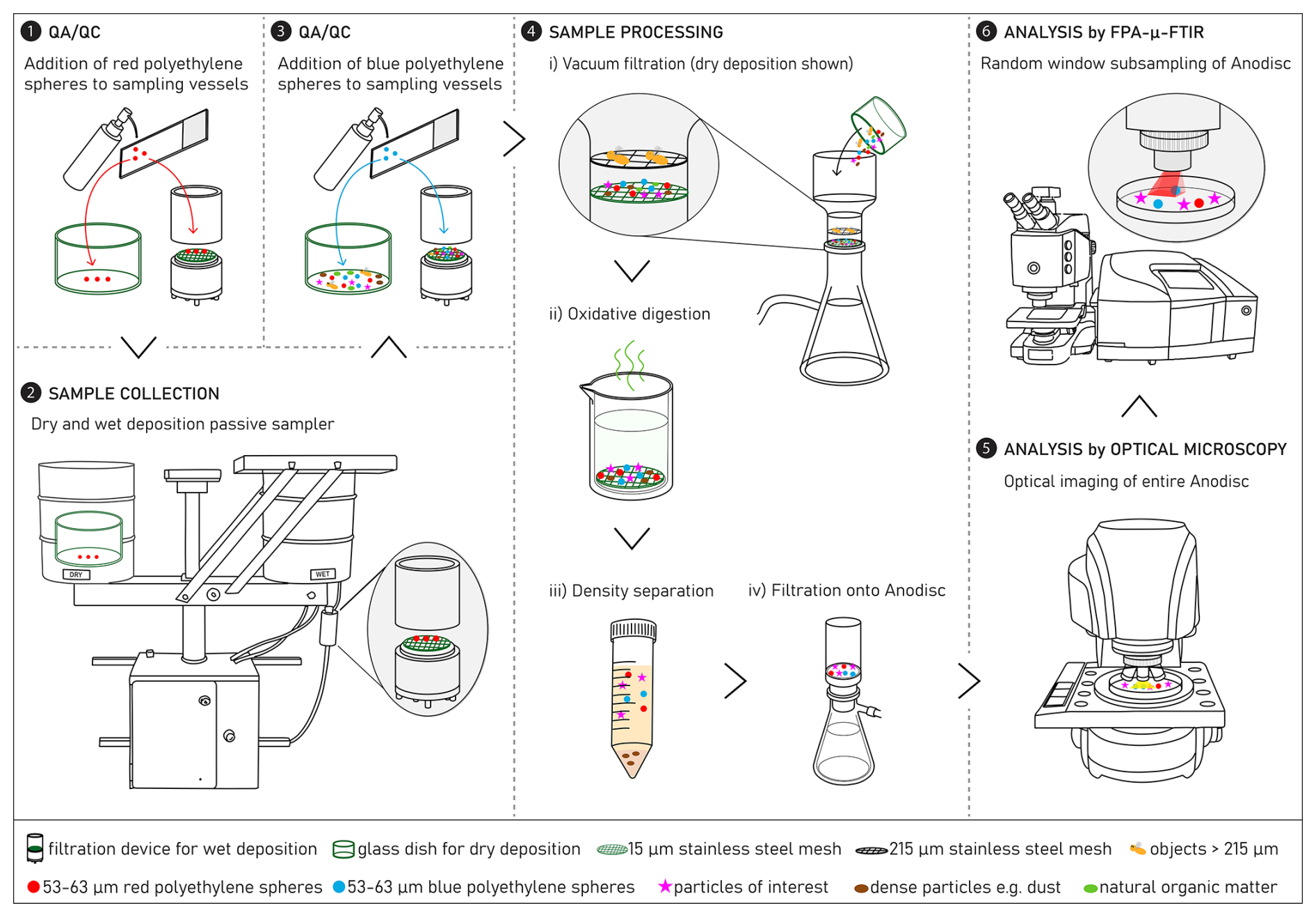
Figure 1 A tailored analytical chain for the quantification of microplastics (MPs) in wet and dry atmospheric deposition samples. The analytical chain includes sample collection (2), processing (4) and analysis by optical microscopy and focal plane array μ-Fourier transform infrared spectroscopy (FPA-μ-FTIR) (5, 6), as well as quality assurance/quality control (QA/QC) (1, 3) using surrogate microplastic standards (red and blue polyethylene spheres, ∅ 53–63 µm).

3 Description of an analytical chain for the quantification of microplastics in wet and dry atmospheric deposition

A schematic of the analytical chain – including sample collection, processing, and analysis, as well as QA/QC steps – developed in this study for the quantification of MPs in wet and dry atmospheric deposition is shown in Fig. 1. Briefly, prior to sample collection, a known number of red PE spheres is added to the respective sampling vessels, i.e. glass dish for dry deposition and aluminium filtration device for wet deposition (step 1, Fig. 1; Sect. 3.5.1). Samples are then collected in a passive sampler (step 2, Fig. 1; Sect. 3.1). After samples are collected and brought to the laboratory, a known number of blue PE spheres is added to the respective dry and wet sampling vessels (step 3, Fig. 1; Sect. 3.5.1). The samples undergo the following processing steps to isolate particles of interest (steps 4i–iii, Fig. 1; Sect. 3.2): size fractionation by vacuum filtration through a series of stainless steel meshes, oxidative digestion to destroy natural organic matter and optionally, density separation to remove heavier particles like mineral dust. The extracted particles are then filtered onto an aluminium oxide membrane (step 4iv, Fig. 1). The aluminium oxide membrane is analysed by optical microscopy (step 5, Fig. 1; Sect. 3.3.1) and focal plane array μ-FTIR spectroscopy (FPA-μ-FTIR) to identify MPs (step 6, Fig. 1; Sect. 3.3.2). Detailed descriptions of each step, including data interpretation, are provided in the following subsections.

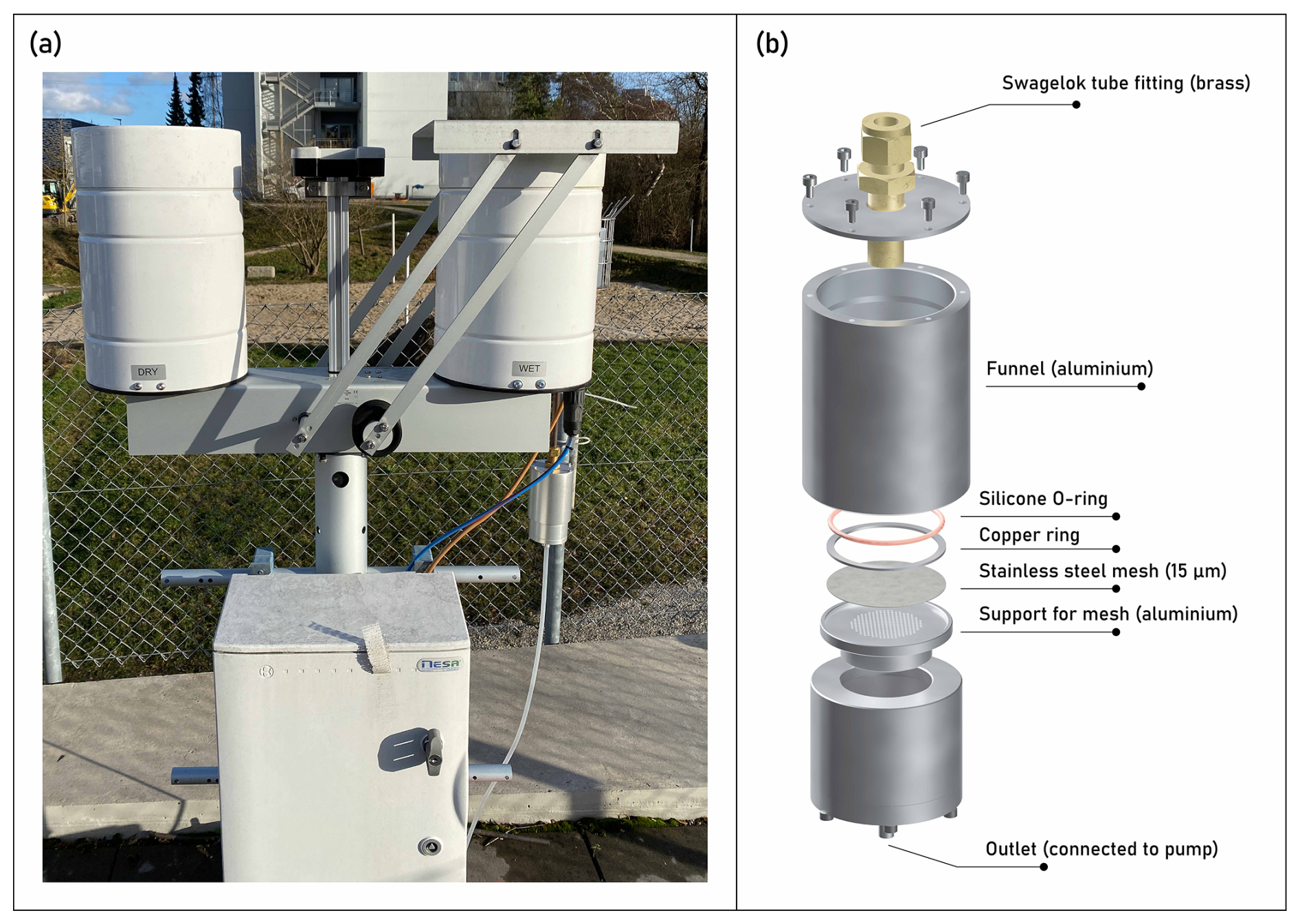
Figure 2 Dry (left cylinder, ∅ 23 cm) and wet (right cylinder, ∅ 23 cm) deposition passive sampler (a). Dry deposition samples were collected in a glass dish (∅ 19 cm) containing a layer of glycerol placed in the cylinder. Wet deposition samples were collected using a custom-made on-site aluminium filtration device (b). The filtration device was fitted with a stainless-steel mesh (∅ 47 mm, 15 µm mesh size).

3.1 Sampling of wet and dry atmospheric deposition

Wet and dry atmospheric deposition were collected with a dedicated passive sampler (Nesa Srl, Italy) (Fig. 2a). Prior to deploying the sampler in the field, the plastic tubing of the sampler was replaced with copper tubing, and the capacitive precipitation sensor was replaced by an optical precipitation sensor (Meteorologische Messtechnik GmbH, Germany) to enable faster switching between wet and dry deposition sampling. A 2 L glass dish (Duran Crystallizing Dish, DWK Life Sciences, Germany) was placed at the (closed) bottom of the cylinder labelled “dry”, to collect gravitationally depositing particles. The bottom end of the cylinder labelled “wet” has a funnel and a copper tube, which guides the precipitation to a custom-made filtration unit made of anodized aluminium (Fig. 2b) installed at the end of the tube. The filtration device was fitted with a stainless-steel mesh (Haver & Boecker, Germany) of diameter 47 mm and mesh size 15 µm to collect particles >15 µm present in rainwater or snow (that melted over time). The mesh size was chosen as this is close to the lower particle size detection limit of 20 µm for (automated) FPA-μ-FTIR spectroscopy (Philipp et al., 2022), the analytical technique of choice in this study. The mesh size may be adapted according to the desired measurement technique and the corresponding particle-size detection limit. The outlet of the filtration device was connected to a membrane pump (FP 70, KNF, Germany) that turned on when the optical rain sensor detected precipitation. This setup enabled the on-site filtration of wet deposition samples directly on stainless-steel meshes, which simplifies subsequent sample processing by eliminating the need of (glass) bottles typically used to collect wet deposition samples. The filtration device was warmed using a heating strip to prevent freezing and facilitate the melting of snow.

For collecting dry deposition samples, we added 70–100 mL of glycerol to cover the bottom of the glass dish and placed it in the cylinder labelled “dry”. The added glycerol served as a particle trap to prevent the remobilization of deposited material under windy conditions, as glycerol is viscous and does not evaporate easily under typical field conditions. Furthermore, after transporting the glass dish back to the lab, deposited particles were easily resuspended by diluting the glycerol in ultrapure water.

The suitability of the setups for collecting wet and dry deposition was assessed through spike-recovery tests using red and/or blue PE spheres (see Supplement, Sect. S1 for full details). The average recovery of red PE particles from the wet deposition sampling setup (filtration device with 15 µm stainless steel mesh) was 98 ± 2 % under laboratory conditions (n=6) and 92 ± 4 % under field conditions (n=3). Recoveries of red and blue spheres from the dry deposition sampling setup (glass dish with glycerol) under field conditions were 87 ± 7 % and 85 ± 6 % (n=3), respectively. These recoveries were considered acceptable for the application of the sampling setup for field monitoring.

To assess its appropriateness for field sampling and for method development purposes, the sampler was installed at a suburban location in Duebendorf, Switzerland [lat: 47°24^′17.5^′′; long: 8°36^′30.5^′′], which is one of Switzerland's National Air Pollution Monitoring Network (NABEL) stations. Wet and dry atmospheric deposition samples were collected at four week intervals. During the transport of samples between the laboratory and the sampling site, the filtration device (containing the filtered wet deposition samples) was sealed with a brass cap (Swagelok, USA), and the glass dish (containing the dry deposition samples and the glycerol) was tightly covered with a wooden lid equipped with a silicone O-ring. The filtration device and glass dish were transported between the field and laboratory in cardboard boxes.

3.2 Sample processing steps

3.2.1 Size fractionation by filtration

After transporting the collected field samples back to the laboratory, the glass dish used for dry deposition samples was rinsed sequentially with pre-filtered ultrapure water and ethanol (see Sect. 3.5.3), and the contents were vacuum filtered through a cascade of stainless steel meshes of two mesh sizes, 215 and 15 µm. An upper mesh size of 215 µm was chosen (1) as it is expected to be large enough to include MPs that can undergo long-range atmospheric transport, but small enough to prevent larger objects, e.g. insects, leaves etc. from overloading samples, and (2) due to challenges in measuring larger particles in transmission mode using FPA-μ-FTIR.

In the case of wet deposition samples, the 15 µm mesh on which particulate wet deposition was collected was first removed from the aluminium filtration device using metal tweezers and placed in a clean 250 mL glass beaker (Duran Beaker, DWK Life Sciences, Germany). The inner surface of the aluminium filtration device was rinsed sequentially with pre-filtered ultrapure water and ethanol over the same beaker. Placing the beaker in an ultrasonic bath for 10 s and subsequently rinsing the steel mesh with water and ethanol, the particulate wet deposition was detached from the steel mesh and resuspended within the beaker. The contents of the beaker were vacuum filtered through a cascade of stainless steel meshes of two mesh sizes, 215 and 15 µm, as done for the dry deposition sample.

3.2.2 Oxidative digestion

After filtration, the 15 µm mesh was placed in a 250 mL glass beaker and underwent oxidative digestion using Fenton's reaction based on a protocol similar to the one described by Philipp et al. (2022). Briefly, 10 mL of hydrogen peroxide, 5 mL ultrapure water, 1 mL 2 mM protocatechuic acid and 1 mL 2 mM iron sulphate were added to the beaker. The beaker was placed in an incubator (Incubator 1000, Unimax 1010, Heidolph, Germany) and allowed to shake at 100 rpm at 40 °C for up to three days. In this step, iron(II) acts as a catalyst to produce hydroxyl radicals from hydrogen peroxide, which can oxidize natural organic matter to produce gaseous carbon dioxide and water. The resulting suspension was finally filtered on the same 15 µm mesh.

3.2.3 Density separation

In samples in which dust was visible to the naked eye after the oxidative digestion step, an additional density separation step was carried out using an SPT solution of density 1.6–1.8 g mL⁻¹ (Philipp et al., 2022). For that purpose, particles remaining on the 15 µm mesh were suspended in ∼ 40 mL SPT solution via ultrasonication, transferred into 50 mL polypropylene (PP) centrifugation tubes (TPP, Switzerland), and centrifuged for 40 min at 2900 g-units. After centrifugation, the particles of interest were separated from denser particles, which formed a pellet at the bottom of the centrifugation tube, by carefully pouring the supernatant and filtering it through the same 15 µm stainless steel mesh. The walls of the centrifugation tube as well as filtration funnel were rinsed using ultrapure water, ensuring that the pellet would not be disturbed and resuspended. The mesh was then placed in the same 250 mL beaker, and the particles on the mesh were resuspended in ultrapure water via ultrasonication. The contents of the beaker were filtered onto an aluminium oxide membrane (∅ 25 mm, 0.2 µm pore size, Whatman Anodisc, Cytiva, Germany), hereafter referred to as an Anodisc filter, for subsequent analysis of MPs.

3.3 Analytical techniques for MP identification and quantification

3.3.1 Optical microscopy

Optical images of the entire Anodisc filters, on which extracted particles were deposited, were recorded at a magnification of either 50× (resolution of ∼ 2.1 µm per pixel) or 80× (resolution of ∼ 1.3 µm per pixel) using an automated optical microscope (VHX-7000, Keyence, Japan). The optical images of the filters were used to obtain information on the spatial distribution of the particles across the entire filter as well as on the size and on the color of each individual particle.

3.3.2 Focal plane array μ-Fourier transform infrared spectroscopy (FPA-μ-FTIR)

To identify MPs on the Anodisc filters, hyperspectral data were recorded using an FPA-μ-FTIR system (64×64 pixel detector, Cary 670 FTIR instrument, Cary 610 IR microscope, Agilent, USA). A 15× IR objective was used which resulted in a resolution of 5.5 µm per pixel and an area of 352 µm ×352 µm for each FPA measurement. All analyses were conducted in transmission mode and covered the wavenumbers between 3900 and 1250 cm⁻¹ at a spectral resolution of 8 cm⁻¹. The measurements were integrated 24 times and the background was integrated 64 times. To account for the time-consuming FPA-μ-FTIR measurements, a random window subsampling method was employed (Jacob et al., 2023). Typically, 11 subsampling windows of 8×8 FPA squares were randomly generated, corresponding to roughly one-third of the filter's analysable area. For each subsampling window, the respective area was (manually) set in focus by adjusting the height of the stage (z-coordinate).

The data from the FPA-μ-FTIR measurements were evaluated using the Microplastics Finder software (Purency, Austria), which is based on a random forest decision algorithm for MP classification (Hufnagl et al., 2019, 2022). Microplastics Finder relies on two proprietary parameters for classification – similarity and relevance – which range from 0 to 1. Similarity describes the quality of the fit between the experimental spectra and the reference spectra of polymers, whereas relevance indicates how confident the model is with the polymer classification. Thresholds for similarity and relevance applied in this study (see Supplement, Table S2) were determined on a polymer-specific basis based on expert judgement, which entailed a visual confirmation that the experimental spectra, obtained through the analysis of real atmospheric deposition samples, agreed well with the reference spectra of the respective polymers.

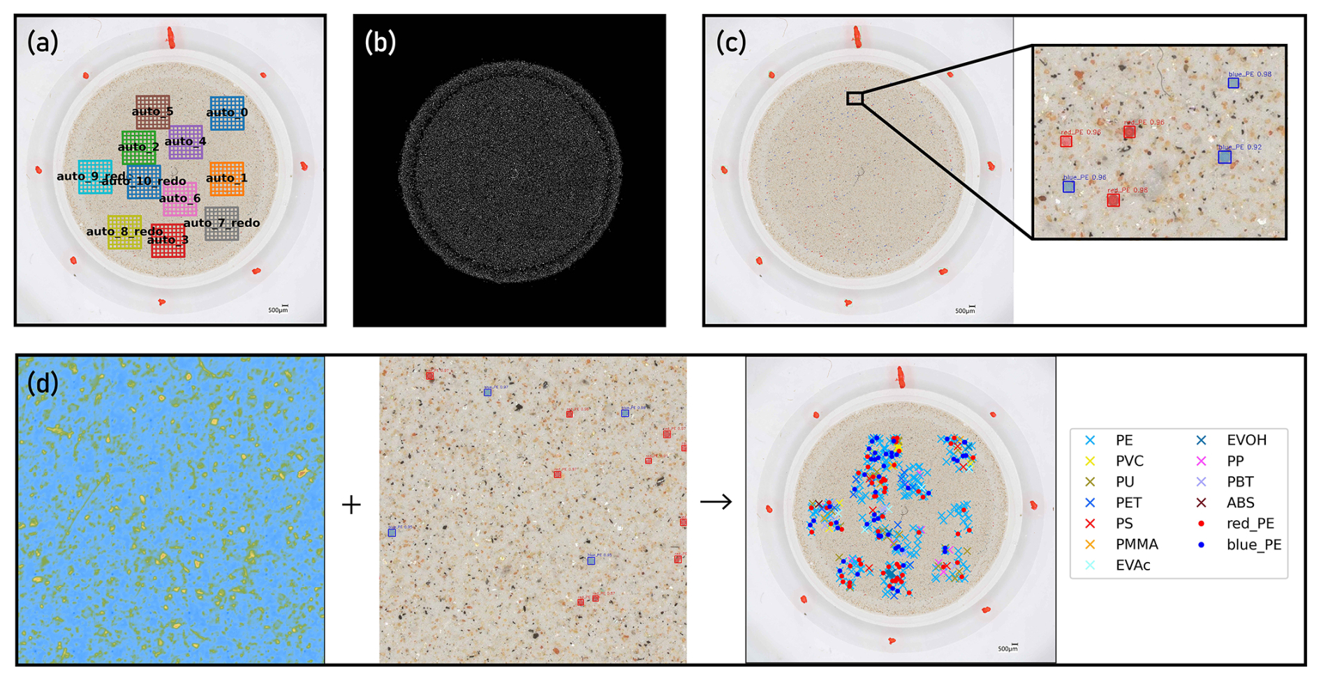
Figure 3 Features of a custom software platform “YAMANAKA” for the quantification of microplastics (MPs) based on correlative optical microscopy and FPA-μ-FTIR spectroscopy. (a) Generation of random subsampling windows across Anodisc filter (optical image shown) for FPA-μ-FTIR spectroscopy; (b) Analysis of the total number of particles on an Anodisc filter based on its optical image (processed image shown); (c) Analysis of the total number of surrogate standards on an Anodisc filter based on its optical image; (d) correlation of results obtained through FPA-μ-FTIR spectroscopy (left panel) and optical microscopy (middle panel) for the calculation of surrogate recoveries as well as determination of environmental MPs in a sample (right panel).

3.3.3 Custom software platform for combining results of optical microscopy and FPA-μ-FTIR

For extracting particle related information from optical microscopy and to correlate images from optical microscopy to chemical images derived from FPA-μ-FTIR measurements, we developed a software environment called “YAMANAKA” in Python.

Key features of YAMANAKA are outlined in Fig. 3 and include: (i) Referencing the coordinates of the optical microscopic image of the filter to the stage coordinates of the FPA-μ-FTIR instrument, thus enabling correlative microscopy, e.g., overlay of optical and chemical (FPA-μ-FTIR ) images, (ii) generating randomized subsampling windows on Anodisc filters for automated FPA-μ-FTIR measurements (Fig. 3a), (iii) detecting individual particles (including non-MPs) on a filter based on optical microscopy images (Fig. 3b), and thereby enabling the quantification of subsampling uncertainties, and (iv) identifying surrogate standards based on optical microscopy (Fig. 3c) and correlating the results to chemical images (Fig. 3d). Based on the latter, recoveries of surrogates were calculated. These features greatly facilitated and streamlined the sample analysis steps of the analytical chain. Further details about YAMANAKA, such as the models used for optical image analyses, are provided in the Supplement (Sect. S3).

3.4 Data interpretation

3.4.1 Microplastic particle size-to-mass estimation

Measurements by FPA-μ-FTIR provide 2D projections of particles from which the length (L), width (W) and area of the particles are derived. These were calculated directly by Microplastics Finder. The area of the particle's 2D projection was used to calculate the circle-equivalent diameter, defined as the diameter of a circle with an area equivalent to the area of the particle's 2D projection. The circle-equivalent diameter was used as the primary metric for reporting particle size.

The values of L and W are defined as the dimensions of the smallest rectangle enclosing individual projected particles. However, there is no information on the third dimension, i.e. the height or thickness (H) of the particles, for which assumptions have to be made.

To estimate the mass of MPs in a given sample, it is often assumed that the particles are of ellipsoidal shape (Barchiesi et al., 2023) and that they are deposited on the filter in their most stable position. Thus, H is smaller than W and L. We used in our study the particle volume calculation done by Simon et al. (2018), which assumes that $H/W$ is equal to the median of the ratio of W and L of all particles in a given sample analyzed by 2D imaging. The volume of an individual MP particle in the sample can then be expressed as:

$$\begin{array}{}\text{(1)}& V_{\mathrm{MP}}={\displaystyle \frac{\mathrm{4}\mathit{\pi }}{\mathrm{3}}}\cdot {\displaystyle \frac{W}{\mathrm{2}}}\cdot {\displaystyle \frac{L}{\mathrm{2}}}\cdot {\left({\displaystyle \frac{W}{L}}\right)}_{\mathrm{median}}\cdot {\displaystyle \frac{W}{\mathrm{2}}}\end{array}$$

The mass of individual MPs was calculated by multiplying the ellipsoid-based volume of the MPs using Eq. (1) with the density of their respective polymer type obtained from selected literature (Bellasi et al., 2021; Caldwell et al., 2022; Horton et al., 2017; Lusher et al., 2020; Huo et al., 2022). The polymer densities applied in this study are available in the Supplement (Table S2). The total mass of MPs in a sample was then calculated by summing the masses of all individual MPs identified in a subsample and extrapolating the mass of the subsample to that of the full sample as outlined for MP numbers in Sect. 4.5.

3.4.2 Determination of atmospheric microplastic deposition rates

Deposition rates, referring to the number or mass of MPs deposited per area and time, were calculated based on the area of the opening of the wet and dry sampling setups (0.042 m²), sampling duration (28 d) and the MP number counts or respective MP masses in the corresponding samples. For mass deposition rates, we assume that the determined distribution of MP particles in the (sub)sample is representative of the true mass distribution of MPs at the measurement location during the measurement period.

3.5 Quality assurance and quality control steps

3.5.1 Positive controls

For field samples, a known number of red PE spheres of 53–63 µm diameter were added to the respective sampling vessels (glass dish for dry deposition and filtration device for wet deposition) before sample collection. After sample collection and after samples had returned to the laboratory, a known number of blue PE spheres of 53–63 µm diameter were additionally added. The procedure for counting and adding the PE spheres to the samples is described in the Supplement (Sect. S1). These added PE spheres served as surrogate standards and were used to quantify sample-specific recoveries, referring to the amount of PE spheres recovered at the end of our analytical chain divided by the amount of PE spheres spiked, as described by Philipp et al. (2022). The use of red and blue PE spheres allowed us to distinguish between losses during sample collection and/or transport versus losses occurring during sample treatment in the laboratory.

3.5.2 Negative controls

Negative controls (n=12), i.e. field- or procedural blanks, were used to quantify contamination levels, and to minimize false positives and false negatives (see Sect. 5). Field- and procedural blanks were handled exactly as the field samples were, except for the exposure to the atmosphere. A procedural blank here refers to a clean stainless-steel mesh placed in a clean 250 mL glass beaker. A wet deposition field blank refers to an aluminium filtration device fitted with a steel mesh taken to the sampling site. A dry deposition field blank refers to a glass dish with glycerol taken to the sampling site.

3.5.3 Measures to limit contamination in the laboratory

To minimize the contamination of samples with MPs from the laboratory, all reagents were filtered through either 0.2 µm polycarbonate membranes (Whatman Nuclepore, Cytiva, Germany) or 15 µm stainless steel meshes before use. All glassware and metallic vessels were muffled for four hours at 450 °C prior to use. A white, cotton lab coat was worn during sample processing. Sampling vessels and other glassware were covered with aluminium foil whenever stored or not actively undergoing treatment.

The use of plastic-based lab equipment was avoided as much as possible. However, for the vacuum filtration step in the laboratory, we used a filtration funnel made of polysulfone. We therefore excluded polysulfone from our analyses of field samples and corresponding blanks.

To monitor potential contamination by airborne MPs in the lab, a clean Anodisc filter was placed in a glass petri dish, which was put on the bench where sample processing steps were carried out, and exposed to laboratory air for six months. The filter was analyzed by FPA-μ-FTIR, which revealed negligible contamination by airborne lab MPs even after six months of exposure, corresponding to <1 MP per filter and day.

4 Assessment of total measurement uncertainty

Each step in the analytical chain described above involves actions that can lead to measurement uncertainties, including random and systematic errors. Measurement uncertainties can be estimated in two main ways – directly by comparing the results of measurements of true replicates, or indirectly by identifying individual components of uncertainties, assessing their standard uncertainties and adding them to obtain a total uncertainty (International Organization for Standardization, 2007).

In this study, the indirect approach was used and the measurement uncertainty of our analytical chain was assessed following the approach of the Guide to the expression of uncertainty in measurement (Joint Committee for Guides in Metrology, 2008). In doing so, three so-called “levels” of uncertainty were quantified. Level 1 (L1) uncertainties refer to those that relate to the direct results of the sample analysis; in this case, the quantification of the number of MPs on an Anodisc filter.

To identify L1 uncertainties, first, the key steps of the analytical chain that contributed to the overall measurement uncertainty on the number of MPs were identified. These were (1) the losses of particles during sample collection, transport and treatment, (2) repeatability of FPA-μ-FTIR measurements, (3) impact of filter topography or differential MP sizes on FPA-μ-FTIR measurement results, (4) (mis)classification of MPs when assigning experimental FPA-μ-FTIR spectra, and (5) subsampling uncertainty during FPA-μ-FTIR measurements. The identified components of uncertainty aligned well with those identified in an interlaboratory comparison study by Ciornii et al. (2025).

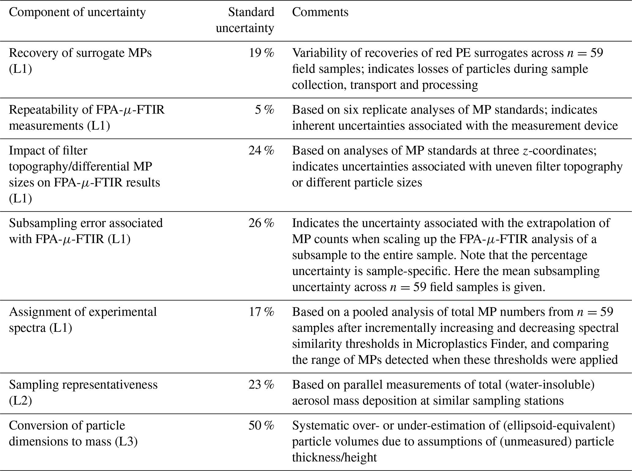
Level 2 and level 3 uncertainties are those arising when additional data extrapolations are made, such as converting the number of MPs on an Anodisc filter to a wet or dry atmospheric deposition rate at a given location (L2) or converting particle numbers and their size and composition information to mass (L3). Table 1 gives an overview of the determined individual components of uncertainty and their standard uncertainties, which are discussed below.

Table 1 Individual components of uncertainty of our analytical chain for the quantification of microplastics in wet and dry atmospheric deposition samples and their relative standard uncertainties. The individual standard uncertainties can be combined to calculate the total measurement uncertainty of the analytical chain (see Sect. 4.8). MPs = microplastics; PE = polyethylene, FPA-μ-FTIR = focal plane array μ-Fourier transform infrared spectroscopy; L1 = level 1 uncertainties related to the quantification of MP numbers on an Anodisc filter; L2 = level 2 uncertainty related to the extrapolation of MP deposition rates; L3 = level 3 uncertainty related to the conversion of MP number and size information to MP mass.

4.1 Recovery of surrogate MPs (L1)

Microplastic particles, including surrogate standards, can adhere to container walls during collection, storage and processing, leading to sample losses along the analytical chain. These losses were estimated by assessing the recovery rates of added surrogate standards, assuming that environmental MPs experience similar losses as the surrogates during transport and processing. Based on the analysis of 59 field samples using the YAMANAKA software, average recoveries of red and blue PE surrogate standards were found to be 65 ± 19 % and 73 ± 20 %, respectively (Table S3). These recovery values and the variabilities are within the range reported in the literature (e.g. Hagelskjær et al., 2023). The variabilities likely reflect manual handling steps, such as rinsing and transferring particles between containers.

The sample-specific recovery of red PE spheres is then used to correct the final MP number in the given sample. However, the variability of recoveries across multiple samples adds uncertainty to such a correction. To illustrate its contribution to the overall uncertainty in MP numbers, we attribute 19 % (Table 1) based on the variability of the recovery of red PE surrogates across 59 samples, as the relative uncertainty associated with particles losses that occurred between sample collection and the end of sample processing (steps 2 to 4 in Fig. 1).

4.2 Repeatability of FPA-μ-FTIR measurements (L1)

To assess the repeatability of FPA-μ-FTIR measurements, we prepared an Anodisc filter on which red PE and blue PS particles were deposited (see Supplement, Fig. S1). An area corresponding to 6 % of the Anodisc's analyzable area, which contained 44 red PE spheres and 22 blue PS spheres, and therefore a total of 66 MP spheres, was analyzed six times consecutively using the same measurement parameters. Figure 4a, b shows the results of six replicate measurements of the same particles (n=66) measured with the same parameters. The total number of red PE and blue PS spheres measured across replicates was variable, and ranged between 59 and 65 particles, with a mean of 62 and a standard deviation of 2.8. This translated into a relative uncertainty of ∼ 5 % (Table 1), i.e. standard deviation ⋅100/mean, which was included in the calculation of the total measurement uncertainty.

4.3 Impact of filter topography or differential MP sizes on FPA-μ-FTIR measurement results (L1)

As our FPA-μ-FTIR spectrometer does not feature an autofocus routine, every individual subsampling area is investigated at a fixed z-coordinate. Variations in the topography of the Anodisc filter and/or MPs of different sizes (heights) therefore result in an over- or under-focused IR beam with respect to the MPs. To quantify the uncertainties related to such changing focal heights (variable degree of defocus of the IR beam), 219 MPs (76 red PE and 143 blue PS spheres, same Anodisc filter as described in Sect. 4.2) were analyzed by FPA-μ-FTIR at three different z-coordinates. The three z-coordinates corresponded to (i) IR beam focused on the filter surface (red PE and blue PS spheres appeared blurry), (ii) IR beam focused ∼ 50 µm above the filter surface (red PE spheres in focus, blue PS spheres slightly blurred) and (iii) IR beam focused ∼ 100 µm above the filter surface (red PE spheres slightly blurred, blue PS spheres in focus). Polyethylene and PS particles were identified based on FPA-μ-FTIR data using Microplastics Finder in combination with YAMANAKA. The numbers of identified red PE and the blue PS spheres were between 53 and 73 (red PE), and 167 and 208 (blue PS) across the measurements (Fig. 4c, d). The results indicated that when the z-coordinates were set such that the IR beam focused 50 or 100 µm above the filter surface, the particles were detected with a higher success rate than when only the surface of the Anodisc was in focus.

The associated relative uncertainty was calculated using the largest deviation in measured particle numbers from the true particle number observed across the three focal height test measurements. This was estimated as 24 % (Table 1), which was included in the estimation of the overall uncertainty of the analytical chain.

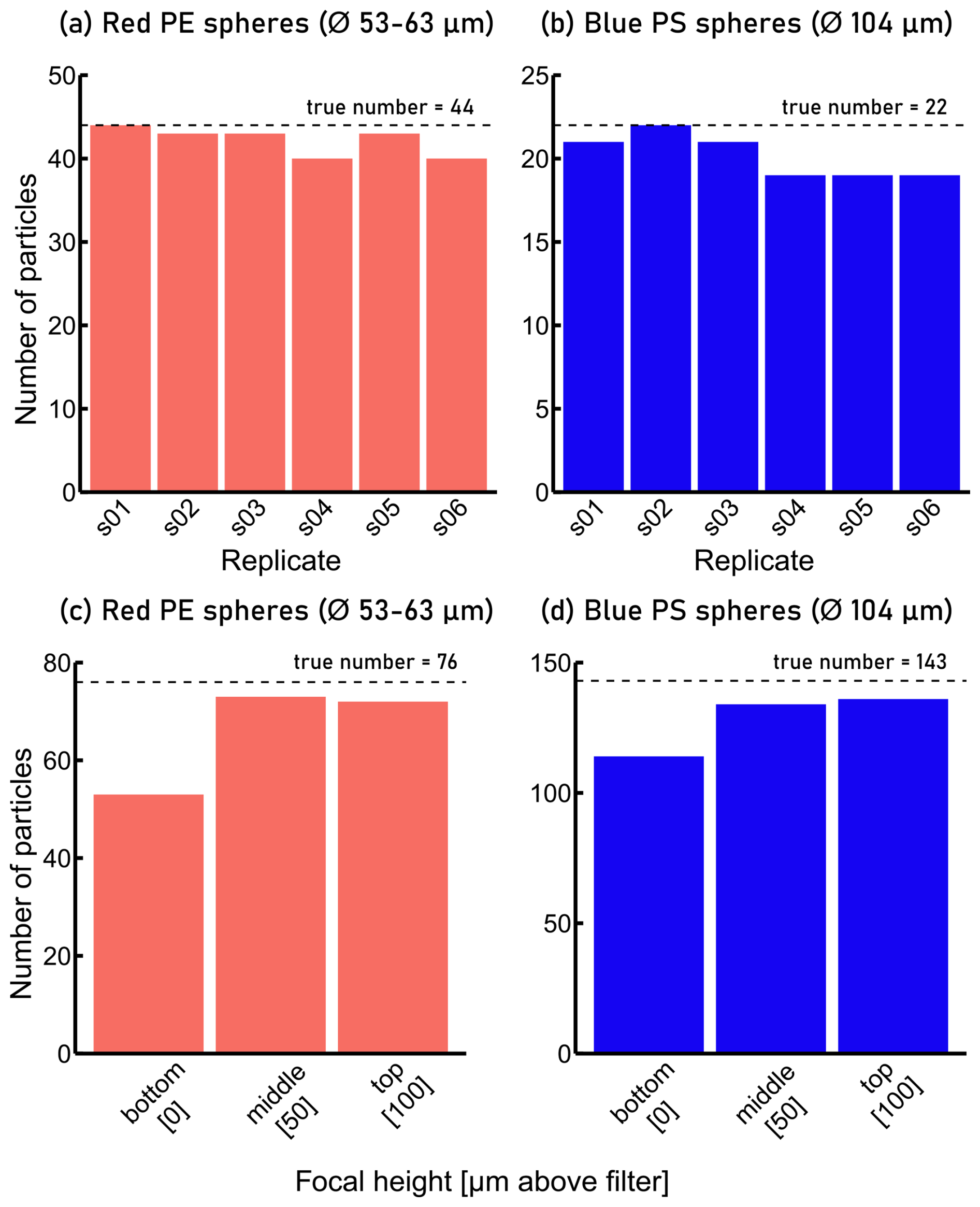
Figure 4 (a) Number of spherical red polyethylene (PE) particles identified during replicate FPA-μ-FTIR measurements compared to the true value of 44 particles observed on an optical microscopy image, (b) number of spherical blue polystyrene (PS) particles identified during replicate FPA-μ-FTIR measurements (true value: 22 particles), (c) number of spherical red PE particles identified during FPA-μ-FTIR measurements at different focal heights (true value: 76 particles), (d) number of spherical blue PS particles identified during FPA-μ-FTIR measurements at different focal heights (true value: 143 particles). In (c) and (d), “bottom”: IR beam focused on the filter surface (red PE and blue PS spheres appeared blurry), “middle”: IR beam focused ∼ 50 µm above the filter surface (red PE spheres in focus, blue PS spheres slightly blurred), “top”: IR beam focused ∼ 100 µm above the filter surface (red PE spheres slightly blurred, blue PS spheres in focus).

4.4 Assignment of experimental FPA-μ-FTIR spectra (L1)

Experimental FPA-μ-FTIR spectra of MPs found in the environment can substantially differ from the FTIR spectra of the respective (pure) polymers that are included in reference databases. Exposure to UV light can for example lead to photooxidation of the MP surfaces, which is reflected in the appearance of a carbonyl peak (Rouillon et al., 2016; Yan et al., 2023). Furthermore, MP particles are often polymer blends composed of more than one polymer type. The assignment of the experimental spectra to specific polymer types is therefore associated with uncertainties and misclassifications cannot be excluded. A quantitative assessment of these uncertainties and degree of misclassifications would require a priori knowledge of the MP types present on the filter substrate. Such information, however, is not available when investigating environmental samples.

Based on expert judgement following a visual comparison in Microplastics Finder of measured spectra of particles identified as plastic with reference FTIR spectra of polymers, we defined similarity thresholds on a polymer-specific basis above which the measured and reference spectra showed good agreement (see Table S2). The thresholds were set such that false positives and false negatives would be minimized.

To determine the uncertainty value arising from the selection of these thresholds, we performed a sensitivity analysis to see how the MP numbers changed if the polymer-specific similarity thresholds were increased or decreased by a value of 0.05, which we considered as realistic variations. The difference in the number of polymers detected with the upper and lower thresholds was calculated for each polymer type. A relative misclassification uncertainty was calculated by first dividing the difference by two and then further dividing this by the detected number of the given polymer at the selected threshold. Table S4 shows total and polymer-specific MP counts at three similarity thresholds (i.e. selected threshold, upper threshold and lower threshold) pooled from the analyses of n=59 environmental samples, together with polymer-specific uncertainties. For reasons of consistency and simplicity, and because not all uncertainties along the analytical chain could be determined for all polymers, we applied the uncertainty value of 17 % (Table 1) calculated across all polymer types rather than polymer-specific uncertainties when calculating the total measurement uncertainty.

4.5 Subsampling error (L1)

Vacuum filtration as we used in our study (step 4i in Fig. 1) can result in uneven deposition patterns of the particles on a filter (Schymanski et al., 2021). An extrapolation of the MP numbers detected in the analyzed subsample to the total number of particles present on the whole filter can therefore lead to a bias in the total amount of MPs present in the individual samples, if the extrapolation is based simply on the area fraction analyzed. We, therefore, applied a scaling approach based on the fraction of particle numbers analyzed as proposed by Schwaferts et al. (2021), which is based on the theory of random sampling.

To apply this approach, the total number of particles on the entire filter (N) and the number of particles in the subsampled windows (S) must be known. These were derived from automated analyses of optical images using the YAMANAKA software. Next, the number of MPs in the subsampled windows (S_MP) was determined from FPA-μ-FTIR measurements in combination with the analysis of spectra by Microplastics Finder. The ratio of MPs to all particles in the subsample $r_{\mathrm{S}}=S_{\mathrm{MP}}/S$ was calculated and considered as representative for the ratio of MPs to all particles deposited on the entire filter. The number of MPs on the entire filter (N_MP) was estimated as:

$$\begin{array}{}\text{(2)}& N_{\mathrm{MP}}=r_{\mathrm{S}}\cdot N\end{array}$$

The determined r_S can be regarded as an estimate of the true ratio of the number of MPs and total number of particles on the entire filter. The relative subsampling error e_rel can be expressed as:

$$\begin{array}{}\text{(3)}& e_{\mathrm{rel}}={\displaystyle \frac{z_{\mathrm{1}-\mathit{\alpha }/\mathrm{2}}\cdot \mathrm{sd}\left(r_{\mathrm{S}}\right)}{r_{\mathrm{S}}}}\end{array}$$

with sd(r_S) the standard deviation of r_S

$$\begin{array}{}\text{(4)}& \mathrm{sd}\left(r_{\mathrm{S}}\right)=\sqrt{{\displaystyle \frac{r_{\mathrm{S}}\cdot (\mathrm{1}-r_{\mathrm{S}})}{S}}\cdot {\displaystyle \frac{N-S}{N-\mathrm{1}}}}\end{array}$$

and $z_{\mathrm{1}-\mathit{\alpha }/\mathrm{2}}$ the $(\mathrm{1}-\mathit{\alpha }/\mathrm{2})$-quantile of the normal distribution, where α denotes the confidence level. For the 95 % confidence level as applied here, α=0.05 and $z_{\mathrm{1}-\mathit{\alpha }/\mathrm{2}}=z_{\mathrm{0.975}}$, which has a value of 1.96. We refer to Schwaferts et al. (2021) for a detailed discussion and derivation of Eqs. (2) and (3).

The sample-specific subsampling uncertainties of n=59 field samples were determined using this approach. On average, the subsampling uncertainty value was 26 % (raw data in Table S3). This average value was used to illustrate the typical contribution of subsampling uncertainty to the overall uncertainty budget of the analytical chain (Table 1). It is noted that when reporting the total uncertainty of a given sample's measurement, the subsampling uncertainty specific to that sample should be used, rather than the average subsampling uncertainty of 26 % mentioned above.

The subsampling uncertainty calculations could indeed also be used prior to FPA-μ-FTIR analysis to optimize measurement time or limit subsampling uncertainty. By estimating the expected proportion of MPs in a sample based on gained experience from prior measurements and calculating the total number of particles in an individual sample via optical image analysis, one could proactively determine the number and size of random subsampling windows that need to be analyzed to achieve a subsampling uncertainty below the desired threshold.

4.6 Representativeness of sample collection (L2)

The heterogeneous wet and dry deposition rates of particulate matter, including MPs, at the local scale additionally contribute to uncertainty when quantifying MPs in atmospheric dry and wet deposition samples. Understanding to what extent the MP content in a wet or dry deposition sample collected in a 0.042 m² catchment area is representative of a larger area, e.g. a measurement station, would require multiple parallel measurements at corresponding scales. Due to the limited number of atmospheric dry and wet deposition samplers available for this study, such measurements were not conducted. Moreover, given the other sources of uncertainties in the quantification of MPs with our analytical chain discussed above (total uncertainty >80 %), it would be challenging to attribute any observed variability in MP numbers across replicates as being caused by unrepresentative sampling.

Therefore, to get an estimate on the intra-site sampling uncertainty, we relied on available data of duplicate measurements of total water-insoluble aerosol deposition taken at four-week intervals from January 2024 to May 2025 at seven stations of the Swiss National Air Pollution Monitoring Network that operate similarly to the one in Duebendorf, where we collected our wet and dry deposition samples. The relative standard deviation of parallel bulk aerosol deposition measurements (rsd_aerosol) was calculated as

$$\begin{array}{}\text{(5)}& {\mathrm{rsd}}_{\mathrm{aerosol}}={\displaystyle \frac{\sqrt{\frac{{\sum }_i^n(x_{i,\mathrm{1}}-x_{i,\mathrm{2}}{)}^{\mathrm{2}}}{\mathrm{2}\cdot n}}}{\frac{\mathrm{1}}{\mathrm{2}\cdot n}{\sum }_i^{\mathrm{2}}(x_{i,\mathrm{1}}+x_{i,\mathrm{2}})}}\end{array}$$

where x_i,1 and x_i,2 are the results of parallel bulk aerosol deposition measurements and n is the number of measurements that have been pooled from the seven sampling locations (n=139). We determined rsd_aerosol=0.23. Based on these data, and assuming that (i) the uncertainty of the bulk aerosol deposition measurements is negligible and (ii) wet and dry MP deposition patterns are similar to that of bulk aerosol deposition, the rsd_aerosol of 23 % can be seen as an estimate for the dependence of the number of measured MPs in the choice of the exact sampling point.

4.7 Estimation of mass (L3)

The L3 uncertainty components are related to the conversion of particle dimensions and numbers to overall MP mass on an Anodisc filter. For such a conversion, the uncertainties associated with the measurement of particle dimensions, estimation of particle volumes and the selection of polymer densities play a role.

4.7.1 Uncertainty in particle size measurements by FPA-μ-FTIR

The uncertainty associated with the determination of particle dimensions (e.g. length and width) by FPA-μ-FTIR was calculated by comparing the diameters of surrogate standards measured by FPA-μ-FTIR versus those measured based on optical microscopy. Based on diameter measurements of n=4452 surrogate standards across 59 atmospheric deposition samples, we identified a systematic underestimation of 9 % by FPA-μ-FTIR (details in Sect. S5). This was taken into account when propagating the error associated with converting particle size to volume and eventually to mass.

4.7.2 Uncertainty in ellipsoid volume estimations

The magnitude of the error to be expected when applying the Simon model (Eq. 1) for particle volume estimations was investigated by Contreras et al. (2024), where a set of 203 plastic particles with sizes of a few millimeters was collected in marine environments and where the size of all three dimensions as well as the mass of the individual particles were measured experimentally. The data set consists of plastic particles of different shapes that could be classified into three classes according to their elongation (1D) (e.g. fibers), flatness (2D) (e.g. films) and uniformity in all three dimensions (3D) (e.g. fragments). Note that the mean size of these particles is larger than five millimeters (length of longest dimension), so these particles cannot be regarded as MPs. Generation of a similar test data set for MP particles is, however, hardly possible.

Contreras et al. (2024) showed that the accuracy of the Simon model strongly depends on the particle shape. For 3D particles, the ellipsoidal shape is a reasonable approximation, and the mass of 3D particles is only slightly overestimated. However, the mass of elongated 1D particles is systematically underestimated, on average by about 44 %. The largest errors occur with the thin 2D particles, for which the calculated thickness H is too large. For a distribution of particle shapes as in the test data set from Contreras et al. (2024) (1D: 44.3 %, 2D: 24.1 %, 3D: 31.5 %), the error in the calculated particle mass is dominated by the overestimation of the mass of the thin 2D particles and about 70 % in total. However, these uncertainty estimations assume that the measured dimensions have no error. Applying the 9 % underestimation of particle dimension described in Sect. 4.7.1. to the data set kindly provided to us by the authors of Contreras et al. (2024), the resulting uncertainty in the particle mass calculation using the Simon model was found to range between an underestimation of 53 % for 1D particles and an overestimation of 142 % for 2D particles. For the distribution of particle shapes as in the test data set of Contreras et al. (2024), the percentage error of MP mass calculation reduces to 29 % (see Sect. S5). Given that the distribution of particle shapes in atmospheric deposition samples is unknown, a conservative but realistic systematic error range of ± 50 % is considered when calculating the MP volume based on the measured number and size information.

4.7.3 Selection of polymer densities

For several polymers, there is a range of densities reported in the literature (see Table S5). To estimate the uncertainties associated with using a specific density when there is a range of possible densities, we selected seven polymers that were frequently detected in our samples – namely PE, polyethylene terephthalate (PET), PP, polyurethane, polymethyl methacrylate, PS and polyvinyl chloride – and listed their respective minimum and maximum density values as reported in selected literature (Bellasi et al., 2021; Caldwell et al., 2022; Horton et al., 2017; Lusher et al., 2020; Huo et al., 2022). The density value we chose when converting the volume to mass was the mean of the minimum and maximum densities reported across those studies. Considering the deviations of the mean from the respective minimum and maximum densities, we calculated polymer-specific percentage uncertainties associated with the use of the mean densities of each polymer when converting volume to mass. The range of uncertainties in the densities of the selected polymers was 2 %–15 %. The most common polymers – PE, PET and PP – had an uncertainty of 5 %. Compared to the large uncertainties of ∼ 50 % associated with volume estimations, we assumed the selection of polymer densities to play a minor role in the total uncertainty of mass estimations and we did not consider it in the overall mass uncertainty calculation.

4.8 Total uncertainty budget

The individual standard uncertainties (u_i, i=1, …, m) of the individual components of L1 uncertainty presented above are assumed to be independent and random. Therefore, the combined standard uncertainty (u) can be expressed as:

$$\begin{array}{}\text{(6)}& u^{\mathrm{2}}={\sum }_{i=\mathrm{1}}^m{u}_i^{\mathrm{2}}\end{array}$$

The expanded measurement uncertainty U of the considered components of uncertainty is then calculated as $U=k\cdot u$ with the coverage factor k. We applied a coverage factor of k=2 so that U corresponds to a confidence level of 95 %.

The uncertainty that is related to the representativeness of the sample collection (L2), which impacts the results when converting the number of MPs in a sample to an atmospheric deposition rate at a given location, can also be assumed to be a random uncertainty. Thus, the expanded measurement uncertainty of atmospheric deposition rates can be calculated from the propagation of L1 and L2 uncertainty components, i.e. including the representativeness of the sample collection as an additional component of uncertainty in Eq. (6).

The L3 uncertainty components related to the conversion of MP particle numbers into mass most likely results in a systematic error, of which the estimation of particle volume has the highest contribution. This is caused by the fact that the actual shape of the particles deviates from the assumed ellipsoidal shape, and the magnitude of over- or under-estimation depends on the actual morphologies of MPs found in samples. Therefore, they cannot be treated as random uncertainties, and the expected systematic error in the conversion from the number to the mass of MPs is considered separately and added to the random measurement uncertainties caused by L1 and L2.

Based on the individual components of L1 uncertainties described in Sect. 4.1 to 4.5, the extended total uncertainty when quantifying MP numbers on an Anodisc filter was determined to be approximately 88 %. Note that the contribution of the subsampling error is sample-specific and therefore the uncertainty of MP numbers in a sample may vary between samples.

Although such a quantitative estimation of total measurement uncertainty for MPs is, to our knowledge, not available in the literature, we could compare the contributions of uncertainty from individual steps in our analytical chain to similar steps identified in the interlaboratory comparison study by Ciornii et al. (2025). For example, the contribution of sample losses during filtration was described as being “high” and estimated at 10 %–30 % (Ciornii et al., 2025). This corresponds well with the average sample losses of 35 % that we observed in our study (based on an average recovery of red PE surrogates of 65 %). It is noted that our losses may be higher because they capture more than only the losses occurring during the filtration step. Similarly, the contribution of “extrapolation of results” was described by Ciornii et al. (2025) as having a “middle-high” contribution. This type of uncertainty corresponds to what we describe as subsampling uncertainty, which on average was 26 % and rather high relative to other components of uncertainty in our analytical chain. “Instrumental settings”, which included the threshold to positively identify spectra by comparison against spectral databases as well as optical focus, were considered to have a “middle-high” contribution (Ciornii et al., 2025). In our case, the assignment of experimental spectra was associated with an uncertainty of 17 % and the influence of focus related to filter topography or differential MP sizes was 24 %, which also translated to middle-high contributions to the total measurement uncertainty relative to other components in our analytical chain. The quantitative assessment of uncertainties carried out in our study therefore agreed well with the qualitative assessment of uncertainties by Ciornii et al. (2025).

The L2 uncertainty component that is related to the representativeness of the sample collection was determined based on co-located measurements of total atmospheric particle deposition and found to be 23 %. Combining this additional L2 uncertainty component with the L1 uncertainties resulted in a total expanded uncertainty of approximately 99 % for the estimation of MP number deposition rates of individual wet and dry atmospheric deposition samples. Note that L1 and L2 uncertainties can be regarded as random uncertainties and the uncertainty for their mean values derived from analyses of a number n of atmospheric deposition samples decreases with the size of n; more specifically, it decreases as a function of the inverse of the square root of n.

For the overall uncertainty of the mass of microplastics in a sample and the associated mass deposition rate, we also apply the relative overall uncertainty of the number of MPs to the calculated total MP mass in the sample. This approach implicitly assumes that the measured size distribution and type of MPs in the collected sample is representative of the true mass distribution of MPs during that sampling time at the sampling location. This results in an uncertainty interval for the calculated total MP mass due to the L1 and L2 uncertainty components. The systematic error caused by converting the MP number into MP mass is then taken into account by assuming a systematic overestimation of the upper limit and a systematic underestimation of the lower limit of the uncertainty interval by 50 % in each case. This leads to the range in which the true MP mass in a sample could lie, given all the uncertainties associated with the measurements, calculations, and assumptions.

5 Critical level (L_C) and limit of detection (LOD) of the analytical chain

The L_C and LOD for the quantification of MP numbers specific to our analytical chain were determined following an approach outlined by Currie (1968). Based on the number of MPs detected in individual blank samples, first the L_C was defined as

$$\begin{array}{}\text{(7)}& L_C={\mathit{\mu }}_B+t_{n-\mathrm{1},\mathrm{1}-\mathit{\beta }}\cdot {\mathit{\sigma }}_B\end{array}$$

where μ_B is the mean number of MPs in n blank samples and $t_{n-\mathrm{1},\mathrm{1}-\mathit{\beta }}$ the 1−β quantile of the t distribution given n−1 degrees of freedom. The L_C is the threshold value above which a signal can be interpreted as “detected” and above which the risk that a measurement of MP is interpreted as an actual signal even though no MP is present (false positives) is minimized. We set the confidence level β=0.05, and therefore $t_{\mathrm{11},\mathrm{0.95}}=\mathrm{1.796}$. Note that the one-sided quantile applies here.

Next, the LOD of the method was considered. While the LOD is often defined as 3σ_B or μ_B+3σ_B, with σ_B being the standard deviation of blank samples (Dawson et al., 2023; Keith et al., 1983), this definition does not take the variance of a real test sample into account and therefore only accounts for Type I errors (false positives) but not for Type II errors (false negatives) (Holstein et al., 2015). We therefore defined LOD as the threshold value above which both false positives and false negatives are minimized, the latter is the risk that an actual signal is incorrectly not recognized as such. The LOD is given as

$$\begin{array}{}\text{(8)}& \mathrm{LOD}=L_C+U_{\mathrm{LOD}}\end{array}$$

with U_LOD being the expanded measurement uncertainty of the measurement of MPs at a signal that is in the range of the LOD (expressed as absolute MP number per sample). With the selection of the confidence level β and the coverage factor used for the calculation of the combined measurement uncertainty (Sect. 4.8), the LOD has a confidence level of 95 %.

Measurements above L_C are a reliable proof of the existence of MPs in the sample and used as the primary reporting limit. Measurements between L_C and LOD should, however, be interpreted carefully, because the increased risk for a Type II error might result in an underestimation of the true MP number in a sample. A more detailed discussion of the chosen approach for the specification of detection limits can be found in Sect. S6.

To determine specific L_C and LOD values for our method, blank samples (n=12) comprising four procedural, four wet deposition, and four dry deposition field blanks, processed identically to environmental samples, were analyzed by FPA-μ-FTIR as described in Sect. 3.3.2. The most frequently observed polymers were PP, PET, and PE, with average counts of 5, 2, and 2 particles per blank, respectively (see Fig. S4). Other polymers appeared at much lower frequencies.

With an average blank value of 13 ± 9 MPs in the analyzed subsamples, an L_C of 29 MPs and LOD of 58 MPs was determined. The average blank value, scaled up for the entire sample, is within the range of blank values reported in the literature and would be considered a medium-level contamination (i.e. average of 10–50 MPs in blanks) according to Lao and Wong (2023). As the polymer-specific particle numbers were low, to ensure a conservative, yet robust, correction across all samples, we integrated the blank values across all polymer types when evaluating the method's L_C and LOD.

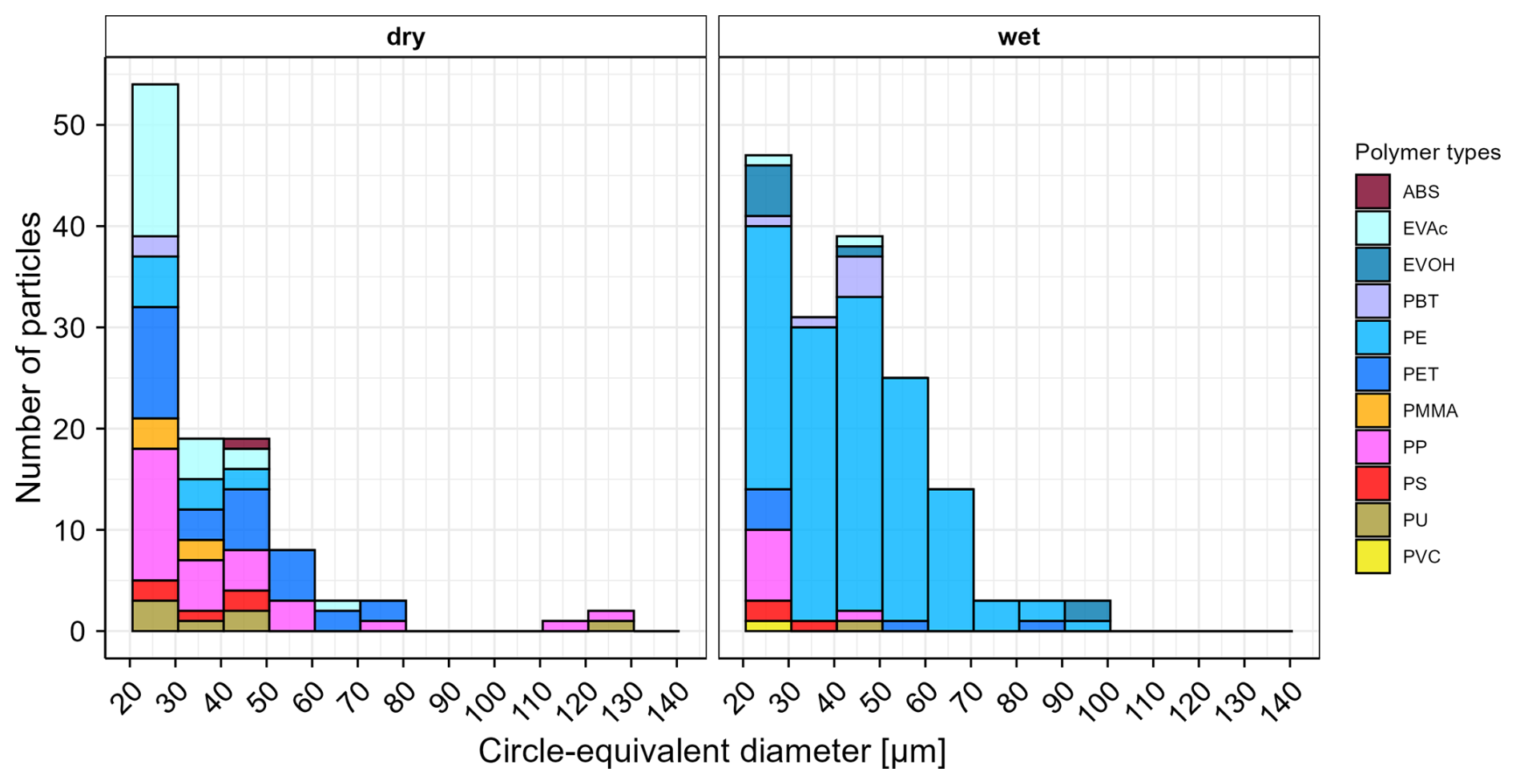
Figure 5 Number of microplastics by polymer type and size detected in the analyzed subsamples of dry deposition (left) and wet deposition (right) samples collected from Duebendorf, Switzerland between 18 July and 15 August 2025. ABS = acrylonitrile butadiene styrene, EVAc = ethylene vinyl acetate, EVOH = ethylene vinyl alcohol, PBT = polybutylene terephthalate, PE = polyethylene, PET = polyethylene terephthalate, PMMA = polymethyl methacrylate, PP = polypropylene, PS = polystyrene, PU = polyurethane, PVC = polyvinyl chloride. Circle-equivalent diameter refers to the diameter of a circle with an area equivalent to the measured area of the particle's 2D projection.

6 Quantitative assessment of MP content in wet and dry atmospheric deposition samples

The above-described analytical chain was used to quantify MPs in monthly samples of wet and dry atmospheric deposition collected during a one-year monitoring campaign at multiple sites. Here, we report specifically on the results for a pair of wet and dry deposition samples collected between 18 July and 15 August 2024, at a suburban site in Duebendorf, Switzerland, to illustrate the strength of our approach. A description of the results of the entire monitoring campaign would go beyond the scope of this study and will be presented elsewhere.

The wet and dry deposition samples were treated according to the steps described in Sect. 3, except for density separation as it was deemed unnecessary. Following sample processing and deposition of extracted particles onto Anodisc filters, the recoveries of surrogate standards for the wet deposition sample were 80 % for both red and blue surrogates, whereas for the dry deposition sample, the recoveries were 81 % for red and 86 % for blue surrogates. The total number of particles (including non-MPs) on the filters were 48 546 and 59 638, respectively for the wet and dry deposition samples. Random subsampling windows contained 15 588 and 18 856 particles (including non-MPs) each and were measured via FPA-μ-FTIR. In the subsampled fractions of the Anodisc filters, 165 (wet deposition) and 109 (dry deposition) MPs were detected. As shown in Fig. 5, the most frequently detected polymer types in the dry deposition sample were PP, PET and ethylene-vinyl acetate, whereas the wet deposition sample was largely dominated by PE.

The associated subsampling errors for these two samples were 13 % and 16 %, respectively. Both number counts were well above the method's critical level L_C of 29 MPs and LOD of 58 MPs. After blank-correcting by subtracting the mean blank value of 13 MPs, the likely numbers of MPs in the analyzed subsamples were determined to be 152 MPs (wet deposition) and 96 MPs (dry deposition). The detected number counts of MPs in the subsamples were scaled to the entire filter area using Eq. (2) and multiplied with factors 1.25 and 1.23 to account for the incomplete recoveries of the red PE surrogate standards. To calculate the total uncertainty in the number count of MPs in the entire wet and dry deposition sample, the sample-specific subsampling error and the remaining L1 uncertainty components listed in Table 1 were propagated to calculate the expanded measurement uncertainty, resulting in 592 (±446) and 375 (±291) MPs for the wet and the dry deposition sample, respectively.

Based on a catchment area of 0.042 m² and sampling duration of 28 d and considering the additional L2 uncertainty related to sampling representativeness, the number-based wet and dry deposition rates were respectively calculated as 528 ± 466 and 335 ± 302 MPs m⁻² d⁻¹. Although the expanded uncertainties of the proposed analytical chain respectively amount to 88 % and 90 % for the wet and dry deposition rate of MPs in these examples, which may seem large, it is essential to have such realistic estimates of measurement uncertainties to correctly interpret measurements and reliably compare results from different (monitoring) studies. In addition, it should be noted that the measurement uncertainty becomes smaller when mean deposition rates are determined from a larger number of samples collected at a given site. Although the interpretation of results from the single samples presented above must be done with care, the deposition rates we calculated for the suburban site in Duebendorf are within the range of values reported in the literature for MPs with particle sizes greater than 20 µm such as in the French Pyrenees (365 with a standard deviation of 69 MPs m⁻² d⁻¹) (Allen et al., 2019), protected areas in Western USA (range of 48–435 MPs m⁻² d⁻¹) (Brahney et al., 2020), Hamburg, Germany (range of 136.5–512 MPs m⁻² d⁻¹) (Klein and Fischer, 2019), London, England (771 with a standard deviation of 167 MPs m⁻² d⁻¹) (Wright et al., 2020), Lanzhou, China (353.83 with a standard deviation of 159.17 MPs m⁻² d⁻¹) (Liu et al., 2022), and South Africa (212 with a standard deviation of 31 MPs m⁻² d⁻¹) (Mutshekwa et al., 2025). It is noted that the studies cited here did not formally calculate measurement uncertainties but rather reported the values (e.g. mean or range of MPs) across a range of samples collected at different times or locations. The studies did not include surrogate standards either.

Finally, MP mass deposition rates of 16 and 7 µg m⁻² d⁻¹ for wet and dry deposition, respectively, were estimated. Based on considerations of L1 and L2 random uncertainties as well as L3 systematic errors, we find corresponding plausible values for the above mass deposition rates to range from 0.94–45.2 and 0.34–20.0 µg m⁻² d⁻¹ for wet and dry deposition, respectively. Few studies have reported mass-based atmospheric deposition rates. Compared to studies by Fan et al. (2022) and Rindelaub et al. (2025), who reported MP mass deposition rates of 334 ± 81 µg m⁻² d⁻¹ (Fan et al., 2022) and 89 ± 9 µg m⁻² d⁻¹ (Rindelaub et al., 2025) at different sites in New Zealand, our results were lower by a factor of 2 or up to 3 orders of magnitude. However, it should be noted that the studies relied on Py-GC-MS measurements for MP classification rather than the μ-FTIR-based approach used in this study and may have targeted different size classes. Moreover, the ranges reported by Fan et al. (2022) and Rindelaub et al. (2025) were not based on measurement uncertainties but rather captured the variability of MP mass deposition rates over multiple sampling sites. Therefore, the observed difference in mass deposition rates may reflect methodological and analytical uncertainties rather than geographical variability. Overall, this underscores the need for future studies to consider method-specific uncertainties and provide reliable ranges of possible values.

7 Conclusion and outlook

We developed an analytical chain for the collection, processing and analysis of MPs in wet and dry atmospheric deposition samples and quantified the uncertainties of each of the steps. Key developments in this work included a tailored setup for the separate collection of wet and dry atmospheric deposition samples, a custom software platform that enabled correlative optical microscopy and FPA-μ-FTIR spectroscopy, and a detailed assessment of the total uncertainty budget associated with the entire analytical pipeline. Although the usefulness of the tailored sampling setup is restricted to researchers seeking to collect atmospheric deposition samples, the software features for analyzing colored surrogate standards and total particle numbers, as well as the considerations used for the determination of the total measurement uncertainty may be applied generally across MP (monitoring) studies regardless of the matrix being investigated.

The total measurement uncertainty of the number of MPs in a single atmospheric deposition sample with our proposed analytical chain was determined to be around 90 %, which was deemed reasonable considering the various steps involved, including several manual steps during sample processing and analysis. The step-by-step assessment of uncertainties identified steps where improvements could be made to reduce uncertainties. In our analytical chain, the most dominant components of uncertainty for the determination of MP numbers were the subsampling error (26 %), influence of topography/different MP sizes on FPA-μ-FTIR measurement results (24 %) and the variable and incomplete recovery of surrogate standards (19 %).

Reducing the subsampling error would require a larger fraction of the filter or ideally the entire filter area to be analyzed, which requires long measurement times in the order of several days. The use of higher throughput instruments, preferably with auto-focus capabilities, could substantially reduce measurements uncertainties in the form of both subsampling uncertainties as well as those caused by a loss of focus due to uneven filter topography or differential particle sizes on the filter. The incomplete and variable recovery of surrogates is likely an indicator of slight differences in sample handling, which is largely unavoidable due to the many manual steps involved in the analytical chain, such as the rinsing of vessels and the transfer of samples from one vessel to another. Such particle losses could be reduced if a closed sample processing device where all sample processing steps could be conducted were available. Additionally, a major source of systematic error when estimating MP mass was the conversion of 2D particle size information from the FPA-μ-FTIR measurements to 3D ellipsoid volumes in the absence of information regarding particle height. Developments in the automated detection of specific particle morphologies such as fibers and the calculation of corresponding cylindrical volumes rather than ellipsoidal volumes could minimize this error.

While many of the uncertainty values are specific to our analytical chain and its operators, the fundamental concepts of our uncertainty assessment are transferable to any analytical chain regardless of matrix. It is important that a careful assessment of all uncertainties is done prior to their application in monitoring MPs.