Aerosol optical-to-microphysical conversion factors for lidars and ceilometers from extended AERONET data analyses: POLIPHON update

Updated POLIPHON (Polarization Lidar Photometer Networking) conversion factors for the laser wavelengths of 355, 532, 911, and 1064 nm are presented. The conversion factors allow us to transfer profiles of aerosol-type-dependent optical properties measured with lidars and ceilometers into profiles of microphysical particle properties, and to estimate cloud condensation nucleus (CCN) and ice-nucleating particle (INP) concentrations at observed cloud levels. These updates were necessary to permit a coherent and harmonized data analysis of different long-term spaceborne lidar observations at 355 and 532 nm and to support ground-based lidar and ceilometer network measurements and research on aerosol–cloud interaction. The POLIPHON conversion factors are obtained by analyzing long-term sun photometer observations conducted at 62 AERONET (Aerosol Robotic Network) stations. Conversion factors are now available for mineral dust, marine aerosol, urban and rural anthropogenic particles, tropospheric and stratospheric wildfire smoke and volcanic sulfate aerosol.

1 Introduction

The POLIPHON (POlarization LIdar PHOtometer Networking) method (Ansmann et al., 2012; Mamouri and Ansmann, 2016, 2017) has been introduced 10–15 years ago to provide an easy-to-handle, robust, lidar-based option to estimate height profiles of particle mass (PM), cloud condensation nucleus (CCN) and ice-nucleating particle (INP) concentration from backscatter lidar profiles. Of key importance are look-up tables of aerosol-type-dependent conversion factors that are derived from global, long-term Aerosol Robotic Network (AERONET, Holben et al., 1998) sun photometer observations that permit the conversion of particle optical into microphysical properties. The importance of such conversion tools arises from the fact that active remote sensing with lidars and ceilometers is the only way to continuously monitor aerosol layers and embedded clouds in the atmosphere with high vertical resolutions. Combined with cloud radar measurements, aerosol lidars provide the grounds for an observation-based in-depth investigation of aerosol–cloud interaction processes. In the framework of satellite-based lidar missions aerosols are characterized on a global scale. Long data sets, covering several decades are meanwhile collected with CALIOP (Cloud-Aerosol Lidar with Orthogonal Polarization, Winker et al., 2009, 2010) from 2006–2023, ALADIN (Atmospheric Laser Doppler Instrument, Baars et al., 2021; Trapon et al., 2025) from 2018–2023, ADCL (Aerosol and Carbon dioxid Detection Lidar, Dai et al., 2024) since 2022, and ATLID (Atmospheric lidar, Wehr et al., 2023; Wandinger et al., 2023) since 2024.

The POLIPHON analysis scheme has been widely applied to analyze spaceborne and ground-based lidar observations of local, regional, and global pollution states, aerosol long-range-transport, and aerosol–cloud interaction (e.g., Ansmann et al., 2011, 2019a, 2025b; Córdoba-Jabonero et al., 2018; Baars et al., 2019; Haarig et al., 2019, 2026; Hofer et al., 2020a; Georgoulias et al., 2020; Jimenez et al., 2020, 2025; Engelmann et al., 2021; Radenz et al., 2021a; Floutsi et al., 2023; Mamouri et al., 2023; Janicka et al., 2023; Shang et al., 2024; Shen et al., 2024; Rogozovsky et al., 2025; Filioglou et al., 2025; Proestakis et al., 2025a, b; Malollari et al., 2025; He et al., 2025b). The broad spectrum of POLIPHON applications have been validated within a variety of field campaigns (e.g., Düsing et al., 2018; Mamali et al., 2018; Haarig et al., 2019; Marinou et al., 2019; Wieder et al., 2022; Choudhury et al., 2022). In this article, we present recent updates and new features of the POLIPHON method. The latest set of conversion factors based on the analysis of sun photometer observations at 62 AERONET sites around the globe is introduced as well.

The following facts and aspects motivated the updates:

1. The aerosol profiling community grew significantly. Besides operational ground-based lidar networks such as EARLINET (European Aerosol Research Lidar Network, Pappalardo et al., 2014) and the mentioned satellite lidar missions, dense ceilometer networks significantly contribute to aerosol profiling on continental scales (e.g., Cazorla et al., 2017; Flentje et al., 2021; Bellini et al., 2024). One of the main ceilometer laser wavelength is 910–911 nm. Consequently, conversion factors are needed that cover the entire laser wavelength spectrum used in active aerosol remote sensing. Therefore, conversion factors for 355, 532, 911, and 1064 nm are presented in this article.

2. The launch of ATLID (laser wavelength of 355 nm) aboard the EarthCARE (Earth Cloud Aerosol and Radiation Explorer, Wehr et al., 2023) satellite in May 2024 prompted us to carefully reevaluate the 355 nm conversion factors, now for five basic aerosol types considered in the POLIPHON look-up tables. Furthermore, to obtain coherent, harmonized time series of global aerosol data sets since the start of the CALIOP satellite lidar, operated at 532 nm, we need updated POLIPHON conversion factor pairs for 355 and 532 nm to combine the CALIOP long-term observations with the EarthCARE measurements and to include even additional long-term observations with ALADIN and the ACDL.

3. The study of Kulkarni et al. (2025) motivated us to improve the statistical analysis applied to obtain the POLIPHON conversion factors. These authors found that our parameterization scheme applied to estimate the CCN concentration n_CCN from the observed particle extinction coefficient σ does not work well and overestimates the CCN concentration in the case of continental aerosol pollution. In our original statistical approach (Mamouri and Ansmann, 2016), we followed the recommendation of Shinozuka et al. (2015) and derived the respective extinction-to-CCN conversion factor from a linear correlation between log(σ) and log(n₅₀) values and between log(σ) and log(n₁₀₀) data, with n₅₀ and n₁₀₀ representing all particles with dry-particle radius > 50 and > 100 nm, respectively. These particle number concentrations are used as proxy for n_CCN. n₁₀₀ is used in the case of dust particles, whereas n₅₀ is used in the case of, e.g., anthropogenic and marine particles. Obviously, our statistical correlation analysis failed because of too noisy n₅₀ and n₁₀₀ data and the impact of outliers, with the consequence that the derived extinction-to-CCN conversion factors were too large. In this study, we apply a weighted linear regression analysis to σ and n₅₀ and to σ and n₁₀₀ data fields in linear scales (York et al., 2004). This approach is better in line with alternative retrieval schemes of Choudhury and Tesche (2022) and Lenhardt et al. (2023) and, most important, efficiently removes unwanted outliers. For all other conversion factors, we used already the linear regression approach in foregoing studies (Mamouri and Ansmann, 2016, 2017; Ansmann et al., 2019b, 2021), however, the improvement here is the removal of outliers.

The paper is organized as follows. In Sect. 2, we briefly explain the POLIPHON method and highlight the changes and improvements compared to the version presented in Mamouri and Ansmann (2016, 2017) and Ansmann et al. (2019b, 2021). In Sect. 3, we introduce the downloaded AERONET data of spectral aerosol optical thicknesses (AOTs) and size distributions and all the AERONET stations we considered in this POLIPHON-update project. We significantly increased the number of AERONET stations involved in the correlation studies to obtain the conversion factors. Even several Arctic and Antarctic AERONET stations are included to derive conversion factors for stratospheric wildfire smoke and volcanic sulfate layers. In Sect. 3.4, we discuss in detail how we handle observations performed at ambient humidity conditions to obtain conversion factors for dry aerosol particles, as requested by the atmospheric modeling community. Number, surface area, and volume concentrations of dry particles are required as input in CCN and INP parameterization schemes. In Sect. 4, all conversion factors for all defined 5 different aerosol types are presented and discussed. A brief conclusion section is given in Sect. 5. The statistical analysis (least-squares estimation (LSE) method) applied to the AERONET observations of optical and microphysical properties is described in Appendix A.

2 POLIPHON method: A compact overview

In this section, we provide a brief overview of the POLIPHON method. More details can be found in Mamouri and Ansmann (2014, 2016, 2017). A detailed description of the POLIPHON technique with focus on dust properties is given in Marinou et al. (2019), Ansmann et al. (2019a, b), and He et al. (2023, 2025a) as well. An extension towards wildfire smoke retrieval was discussed in Ansmann et al. (2021). The principle idea, concept, and data analysis scheme of the POLIPHON is illustrated in Fig. 1. The aerosol types considered in the updated POLIPHON data analysis are listed in Table 1.

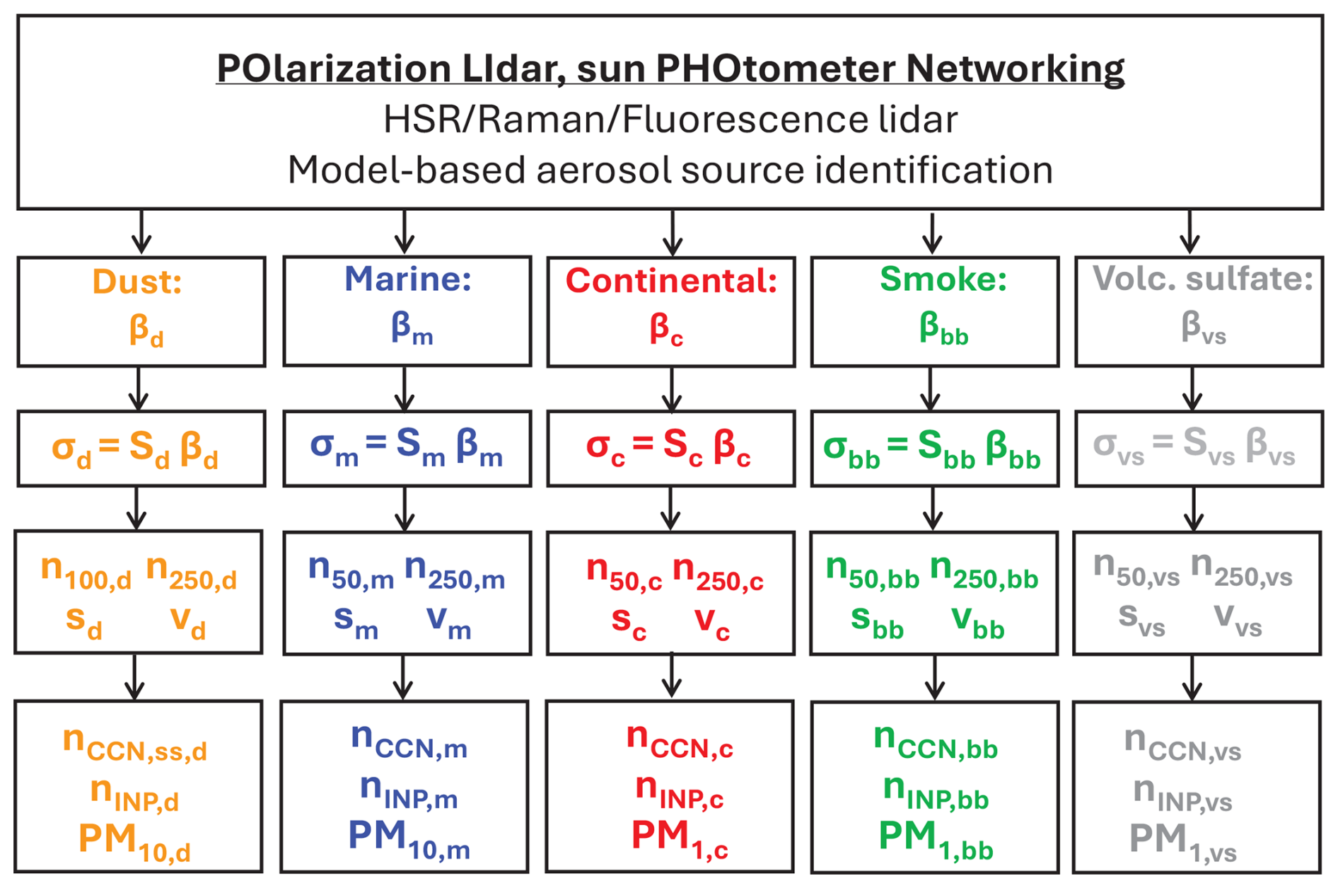
Figure 1 The POLIPHON approach to derive microphysical and cloud-process-relevant aerosol properties of five aerosol types (listed in the 4th and 5th row) from lidar observations of optical properties (backscatter and extinction coefficients β_i and σ_i, respectively, linked by the extinction-to-backscatter ratio S_i). In the identification of the aerosol types, aerosol transport modeling is used as well. The different data analysis steps and listed aerosol parameters are explained in the following Sect. 2.1 to 2.5.

Table 1 Aerosol types considered in the determination of updated POLIPHON conversion factors. Besides the main aerosol types, marine aerosol, mineral dust with fine-mode (df) and coarse-mode (dc) fraction, and continental anthropogenic haze, we consider biomass burning (bb) smoke and volcanic sulfate (vs) in the troposphere and UTLS.

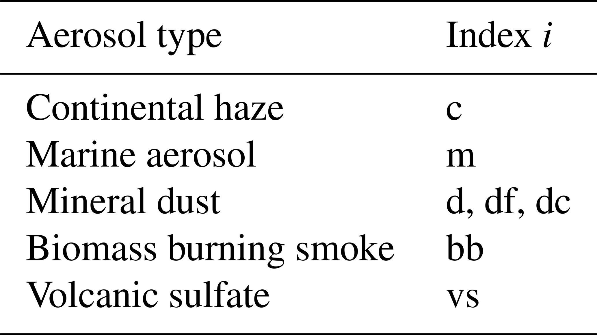
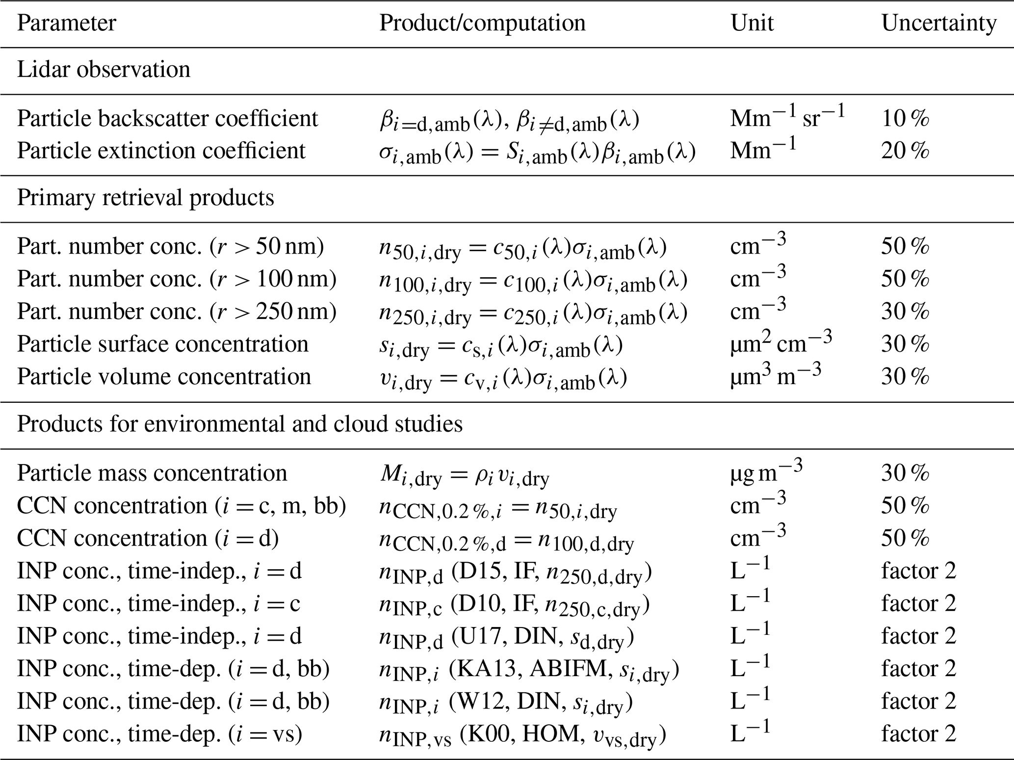
Table 2 Overview of the computations and conversions within the POLIPHON data analysis. The primary retrieval products ($n_{\mathrm{50},i,\text{dry}}$ to $n_{\mathrm{250},i,\text{dry}}$, s_i,dry, v_i,dry) for dry aerosol conditions are calculated from aerosol-type-dependent particle extinction coefficients σ_i,amb(λ) observed at ambient conditions (index: amb) and laser wavelength λ. r denotes particle radius. The dry-aerosol products are requested input data in the particle mass estimation and CCN and INP parameterizations (products for environmental and cloud studies). Details to CCN estimations and the different ice nucleation modes (IF, ABIFM, DIN, HOM) as well as the relevant literature for the respective parameterizations (D10, D15, U17, KA13, W12, K00) are given in the text. The units (column 3) are given for the products (β, σ, n, s, v, M, n_CCN, n_INP). Typical uncertainties, gained from many field studies and simulations, are listed in row 4.

2.1 Step 1: Separation of dust and non-dust optical properties

The POLIPHON data analysis consists of five steps. An overview of the main retrieval packages is shown in Table 2. In the first step, the dust and non-dust contributions to the particle backscatter coefficient are separated by using the measured profile of the particle linear depolarization ratio (Tesche et al., 2009; Mamouri and Ansmann, 2014). However, this is only possible if a polarization-sensitive lidar or ceilometer is operated. Besides non-spherical dust particles, volcanic ash, wildfire smoke in the upper troposphere and lower stratosphere (UTLS) and dry marine particles in the shallow marine boundary layer can cause enhanced light depolarization (Ansmann et al., 2010; Haarig et al., 2017, 2018). However, by using backward trajectory analysis these contributions to the measured depolarization ratio can be easily identified so that a clear quantification of the dust backscatter coefficient is possible. Step 1 is important because mineral dust belongs to the key aerosol types in the atmosphere and influences cloud processes in a very specific way as will be discussed below. If a polarization-sensitive lidar instrument is not available, one may use available modeled aerosol profile information to estimate the dust backscatter fraction, as described in the next section.

2.2 Step 2: Identification of the aerosol types

Aerosol-type and aerosol source information for detected aerosol layers can be generally obtained, e.g., via height-resolved air mass source attribution (Radenz et al., 2021b), backward trajectory analysis (Stein et al., 2015), or from large-scale atmospheric simulations with the CAMS (Copernicus Atmosphere Monitoring Service) model. CAMS is a global atmospheric composition forecast production system (Amarillo et al., 2024). Furthermore, simultaneously measured extinction and backscatter profiles observed with Raman lidar or High Spectral Resolution Lidar (HSRL) can be used to identify the non-dust aerosol types in the observed layers (Giannakaki et al., 2020) when using a polarization lidar.

Complex mixtures of aerosols, as they may frequently occur in coastal polluted areas near deserts as for example in the Eastern Mediterranean (Rogozovsky et al., 2025), are probably the most difficult scenarios regarding a proper identification of all contributing aerosol types. However, in the majority of aerosol scenarios, the aerosol conditions are much more simple, as numerous lidar observations of well-defined lofted desert dust plumes, pronounced wildfire smoke layers, marine aerosols over the remote oceans, or of the anthropogenically polluted boundary layer over the industrial continents show.

Note that conversion factors for volcanic ash are not included in Table 1. The volcanic ash conversion factors are very similar to the ones for mineral dust as observations showed (Ansmann et al., 2011).

2.3 Step 3: Conversion of aerosol-type-dependent backscatter into extinction coefficients

In the third step, the aerosol-type-dependent components β_i(λ) of the observed particle backscatter coefficient must be converted into respective particle extinction coefficients σ_i(λ) by using published data sets of aerosol-type-dependent extinction-to-backscatter ratios or lidar ratios S_i(λ) (Müller et al., 2007; Groß et al., 2013; Haarig et al., 2018, 2025; Floutsi et al., 2023, 2024). Meanwhile, many publications for lidar ratios at λ = 355 and 532 nm, and a few reports for the wavelength of 1064 nm are available in the literature (Haarig et al., 2022, 2025). The new generation of space lidars (355 and 532 nm HSRLs), measuring both the backscatter and the extinction coefficient of a given aerosol mixture, is able to produce its own aerosol-type-dependent lidar-ratio climatology by analyzing the observations, e.g., in pure dust or pure marine regions, in dense wildfire smoke plumes (Haarig et al., 2026), or highly polluted urban areas.

2.4 Step 4: Conversion of aerosol-type-dependent extinction coefficients into microphysical properties

In the fourth step, the POLIPHON extinction-to-number conversion factors c_50,i(λ), c_100,i(λ), and c_250,i(λ), the extinction-to-surface-area conversion factors c_s,i(λ), and the extinction-to-volume conversion factors c_v,i(λ) are applied to convert the lidar-derived aerosol-type-dependent extinction coefficients σ_i(λ) into particle number concentration n_50,i (considering all particles with dry-particle radius > 50 nm), n_100,i (considering all particles with dry-particle radius > 100 nm), and n_250,i (considering all particles with dry-particle radius > 250 nm), and into surface area (s_i) and volume concentrations (v_i). Table 2 (primary retrieval products) provides an overview of these conversions. The dry-aerosol products (index: dry) are required as input in the estimation of particle mass, CCN, and INP concentrations. The dry-aerosol properties are, however, derived from extinction coefficients σ_i,amb(λ) measured at ambient humidity conditions (Index: amb). The impact of water uptake by aerosol particles is small and thus the uncertainty introduced by unknown water uptake effects as long as the relative humidity (RH) is < 70 %. Aerosol particles can be regarded as dry at RH < 50 %. At RH > 75 % significant water uptake occurs in the case of hygroscopic particles such as anthropogenic sulfate particles (Skupin et al., 2016). Atmospheric conditions with RH > 75 % are particularly relevant for aerosol observations in the vicinity of clouds, where retrieving aerosol microphysical characteristics accurately is key to properly studying aerosol–cloud interaction. The water-uptake impact must thus be considered in the POLIPHON data analysis. This aspect is further discussed in Sect. 3.4.

According to Table 2, the conversion factors are designed in such a way that the required dry-particle microphysical products can be directly obtained from the observations (conducted at ambient conditions). Besides the number, surface, and volume concentrations in Table 2 further products are computed in the case of dust, such as $n_{\mathrm{60},\mathrm{d},\text{dry}}$, $s_{\mathrm{100},\mathrm{d},\text{dry}}$, v_dc,dry, and v_df,dry. The quantities will be explained in Sect. 3.1.

2.5 Step 5: Estimation of mass concentrations and cloud-relevant products

In the fifth and final step of the POLIPHON data analysis, the aerosol products, which are of importance for environmental monitoring and studies of aerosol–cloud interaction, are calculated. The dry-particle mass concentration M_i,dry is obtained from the derived volume concentration v_i,dry in combination with particle density information. The particle densities ρ_d, ρ_c, ρ_m, and ρ_bb for dust, continental aerosol pollution, dry marine particles, and wildfire smoke particles are set to 2.6, 1.5, 2.16, and 1.15 g cm⁻³, respectively (Ansmann et al., 2012, 2021). The particle density for stratospheric sulfate particles ρ_vs is a strong function of temperature (Wandinger et al., 1995). The H₂SO₄ concentration of the sulfuric acid-water solution droplets can be calculated by using model-based temperatures and by assuming a typical water vapor concentrations, e.g. of 5 ppm in the dry lower stratosphere.

An important POLIPHON application is the estimation of CCN and INP concentrations in the vertical profile up to tropopause level. Dust particles play a special role in aerosol–cloud-interaction processes. They are omnipresent in the atmosphere (Froyd et al., 2022). On the one hand, pure dust particles are hydrophobic in contrast to other relevant aerosol types, such as marine or anthropogenic pollution particles. Thus, dust particles seem to be quite inefficient CCN (Kumar et al., 2009; Koehler et al., 2009; Choudhury et al., 2026) as long as they are not internally mixed with soluble, hygroscopic material. For hydrophobic dust particles, the dust particle number concentration n_250,d may be regarded as an appropriate proxy for the dust CCN reservoir (Kelly et al., 2007).

During long-range transport, chemical aging (Tang et al., 2016) and cloud processing (Wurzler et al., 2000) lead to a coating of dust particles by soluble material (Karydis et al., 2011, 2017). This aspect was already discussed by Mamouri and Ansmann (2016). Contaminated dust particles are very efficient CCN, because they are comparably large and hygroscopic. For these particles n_100,d is a good CCN proxy. Even smaller dust particles may serve as CCN after accumulation of hygroscopic substances so that n_60,d may be regraded as an overall proxy for the dust CCN reservoir.

It should be emphasized in this context, that the light depolarization characteristics of the contaminated, irregularly shaped dust particles is not affected (compared to the ones of pure dust particles showing no contamination) as long as RH indicates dry conditions (RH < 60 % to 70 %). This is the clear conclusion of our field-campaign and long-term studies in highly polluted environments such as Cabo Verde during the winter season (Tesche et al., 2009) and at Dushanbe in Tajikistan (Hofer et al., 2020a, b). An accurate separation of dust and non-dust fractions is possible even in cases with aged and internally mixed dust particles. This conclusion is supported by accompanying sun photometer observations, i.e., by the good agreement between sun-photometer-derived fine- and coarse-mode AOTs and the lidar-derived dust and non-dust AOTs. Complex mixtures of dust and anthropogenic pollution can be regarded as an external mixture of contaminated dust and haze particles.

The number concentrations $n_{\mathrm{50},i,\text{dry}}$ and $n_{\mathrm{100},\mathrm{d},\text{dry}}$ in Table 2 (primary POLIPHON products) are used as CCN proxies $n_{\text{CCN},\mathrm{0.2}\mathit{\%},i}$ for hygroscopic (i = c, m, bb) and hydrophobic (dust, i = d) particles, respectively, for a typical water supersaturation of 0.2 % (relative humidity over water of 100.2 %). Such a supersaturation is reached during updraft conditions with low vertical velocities of clearly below 1 m s⁻¹. At stronger updraft speeds and correspondingly higher supersaturation values of 0.4 % to 0.7 %, the n_CCN values may be a factor of 5–10 higher than the ones for 0.2 % as we pointed out in Mamouri and Ansmann (2016).

Mineral dust is the most important INP type (DeMott et al., 2015; Kanji et al., 2017). Two different INP parameterization concepts are discussed in the literature and used in simulation models, the time-independent (diagnostic) approach and the time-dependent (prognostic) approach (Knopf et al., 2023). The time-independent approach includes a time-independent particle-number- and surface-area-based descriptions of ice nucleation (DeMott et al., 2010, 2015; Ullrich et al., 2017), denoted as D10, D15, and U17, respectively, in Table 2. The particle number concentration $n_{\mathrm{250},\mathrm{c},\text{dry}}$ (considering continental, insoluble particles with radius > 250 nm) is used as aerosol input in the D10,IF parameterization scheme to estimate the INP concentration in the case of immersion freezing (IF). Immersion freezing means that nucleation occurs on an insoluble particle which is immersed in a cloud water droplet (DeMott et al., 2010). The dust particle number concentration $n_{\mathrm{250},\mathrm{d},\text{dry}}$ is used as aerosol input in the D15,IF parameterization scheme used to estimate the dust INP concentration (DeMott et al., 2015). Ullrich et al. (2017) provides a deposition ice nucleation (DIN) parameterization for dust particles. DIN (ice nucleation initiated by water vapor deposition on INPs) typically occurs at cirrus level and temperatures < −40 °C. The dust surface area concentration s_d,dry is the aerosol input. Further diagnostic INP parameterization for marine particles (McCluskey et al., 2018), biological aerosol components (Tobo et al., 2013), and organic particles (Tobo et al., 2014) are available, but not listed in Table 2. Aerosol input is always the surface area concentration.

The time-dependent approach to immersion freezing is following the classical nucleation theory (CNT) (Pruppacher and Klett, 1997; Knopf and Alpert, 2013; Alpert and Knopf, 2016; Knopf et al., 2023). In the time-dependent approach, all particles can be activated at a random base and belong to the reservoir of INPs within a given cloud layer. Aerosol-type-dependent nucleation rates control the nucleation of ice crystals per second (Knopf et al., 2023). According to DeMott et al. (2010, 2015) and Schneider et al. (2025) the large particles with radius > 250 nm are the most favorable INPs. We may thus introduce the number concentration $n_{\mathrm{250},i,\text{dry}}$ as INP reservoir proxy. In Knopf and Alpert (2013) (KA13, ABIFM: water-activity based immersion freezing model) and Wang et al. (2012) (W12, DIN), time-dependent INP parameterizations for immersion freezing and deposition ice nucleation, respectively, are described.

Finally, an INP parameterization for homogeneous freezing is listed (Koop et al., 2000) (K00, HOM). This ice nucleation mode describes freezing of liquid sulfate particles (background aerosol particles or volcanic sulfate particles in the upper troposphere) at temperatures below −40 °C. Here, the volume concentration v_vs is the aerosol input parameter. Note, that all ice nucleation processes are strong functions of temperature, relative humidity, and vertical wind conditions (creating the ice supersaturation conditions required to start ice crystal nucleation). More discussion on INP retrieval and estimation with focus on lidar INP profiling are given in Mamouri and Ansmann (2016) and Ansmann et al. (2019b, 2021, 2023, 2025a).

3 POLIPHON conversion factors from AERONET observations

3.1 Data analysis concept

Main goal of the article is to present an updated set of POLIPHON conversion factors c_50,i(λ), c_100,i(λ), c_250,i(λ), c_s,i(λ), and c_v,i(λ) for five different aerosol types, defined in Table 1, and four lidar/ceilometer laser wavelengths. The POLIPHON conversion factors required in Table 2 are obtained from statistical analyses (explained in the Appendix A) of the correlation between two data records x_i,j(λ) and y_i,j. For simplicity, we assume dry-aerosol conditions in this introductory section. In Sect. 3.4, we explain the procedure for the general case of AERONET observations at ambient humidity conditions. The data set x_i,j(λ) contains all individual observations (from j=1 to N_obs) of the aerosol optical thickness AOT_i,j for wavelength λ and aerosol type i measured at one of the selected AERONET sites. The data set y_i,j contains the column-integrated values of one of the microphysical retrieval products such as $\int n_{\mathrm{50},i,j}\left(z\right)\mathrm{d}z$, $\int n_{\mathrm{250},i,j}\left(z\right)\mathrm{d}z$, $\int s_{i,j}\left(z\right)\mathrm{d}z$, or $\int v_{i,j}\left(z\right)\mathrm{d}z$ with height z above the AERONET station.

The AERONET data base stores all individual observations of the AOT from 340 to 1640 nm and the related column-integrated particle size distribution for all AERONET sites (AERONET, 2026; Sinyuk et al., 2020). The size distributions are obtained by applying a well-designed and validated comprehensive inversion scheme (Dubovik and King, 2000; Dubovik et al., 2000, 2006) to the spectrally resolved AOT observations and the measured spectral sky radiances. From the particle size distributions, the column-integrated properties $\int n_{\mathrm{50},i}\left(z\right)\mathrm{d}z$, $\int n_{\mathrm{250},i}\left(z\right)\mathrm{d}z$, ∫s_i(z)dz, and ∫v_i(z)dz, are calculated in the first step of the data analysis to obtain the POLPIHON conversion factors. Details are given in Mamouri and Ansmann (2016, 2017). As will be presented in the next section, we selected preferably AERONET sites with long-term observation over more than 10 years and thus having data records of the order 1000–100000 individual observations of optical and corresponding microphysical properties.

In the next step, a linear regression is applied for a well-defined subgroup of AERONET observations, e.g., for all dust-dominated observations (aerosol type index i = d) collected at a given near-desert station. The statistical analysis is repeated for all selected AERONET stations within or close to a desert. The applied least-squares estimation (LSE) method (York et al., 2004), described in the Appendix A, considers all individual dust observational data sets AOT_d,j(λ), $\int n_{\mathrm{100},\mathrm{d},j}\left(z\right)\mathrm{d}z$, $\int n_{\mathrm{250},\mathrm{d},j}\left(z\right)\mathrm{d}z$, $\int s_{\mathrm{d},j}\left(z\right)\mathrm{d}z$, and $\int v_{\mathrm{d},j}\left(z\right)\mathrm{d}z$), collected at one station. For each data set consisting of pairs of a given AOT_i,j(λ) and one of the defined microphysical products, e.g., of the dust particle volume concentration v_d,j, the linear regression analysis is performed and yields the conversion factor, e.g., the dust extinction-to-volume conversion factor c_v,d(λ) as needed in Table 2. For dust, the linear regression analysis is performed with 8 different microphysicial properties ($\int n_{\mathrm{60},\mathrm{d},j}\left(z\right)\mathrm{d}z$, $\int n_{\mathrm{100},\mathrm{d},j}\left(z\right)\mathrm{d}z$, $\int n_{\mathrm{250},\mathrm{d},j}\left(z\right)\mathrm{d}z$, $\int s_{\mathrm{d},j}\left(z\right)\mathrm{d}z$, $\int s_{\mathrm{100},\mathrm{d},j}\left(z\right)\mathrm{d}z$, $\int v_{\mathrm{d},j}\left(z\right)\mathrm{d}z$, $\int v_{\text{df},j}\left(z\right)\mathrm{d}z$, and $\int v_{\text{dc},j}\left(z\right)\mathrm{d}z$). In all other cases (marine and continental aerosol, wildfire smoke, and volcanic sulfate), four regression studies are conducted per wavelength with AOT_i,j(λ) and with one of the four defined microphysical products $\int n_{\mathrm{50},i,j}\left(z\right)\mathrm{d}z$, $\int n_{\mathrm{250},i,j}\left(z\right)\mathrm{d}z$, $\int s_{i,j}\left(z\right)\mathrm{d}z$, and $\int v_{i,j}\left(z\right)\mathrm{d}z$.

The long list of 8 dust conversion factors is related to specific role of dust in cloud processes. Freshly emitted hydrophobic dust particles may be rather inefficient CCN. Only particles with radius > 100 nm or even larger ones, partly > 200 nm in radius, may be able to serve as CCN. However, dust particles coated with hygroscopic substances may act as CCN already at radius sizes of > 50–60 nm. With $n_{\mathrm{60},\mathrm{d},\text{dry}}$, we introduce a new CCN proxy for contaminated dust, e.g., dust particles with sulfate coating.

In the case of ice nucleation, the surface area concentration s_d is usually the input parameter in INP parameterization. However, in immersion freezing processes with hydrophobic dust INPs, only the surface area concentration of the activated CCN (n_100,d) inside the droplets is then relevant in heterogeneous ice nucleation processes, i.e., the surface area s_100,d considering only the dust particles with radius > 100 nm should be used as aerosol input pararmeter in the INP parameterizations.

For a number of reasons summarized by Proestakis et al. (2025a, b), especially when illuminating the life cycle of dust in the atmosphere, lidar-derived profiles of fine-mode and coarse-mode dust mass concentrations are useful to improve parameterizations of dust emission, long-range transport and deposition in atmospheric models. Lidar-model comparisons regarding fine-mode and coarse-mode fractions during long-range transport were discussed in Ansmann et al. (2017). Therefore, we include extinction-to-volume conversion factors for fine mode c_v,df and coarse mode c_v,dc.

For a given station (assigned to one of the five aerosol types), the regression analysis is repeated for each of the different 4–8 microphyscial products to obtain the respective set of 4–8 conversion factors. This procedure is repeated for each of the four wavelengths. In the final step, we averaged all station-by-station conversion factors (for a given aerosol type, wavelength, and microphysical product) to obtain the mean conversion factors for all defined aerosol types and wavelengths. In the next two sections, we introduce the selected 62 AERONET stations and how we filtered the AERONET data sets to obtain the aerosol-type-dependent AERONET data sets required as input in the regression analyses.

Table 3 Overview of 62 AERONET stations, selected to obtain the conversion factors for mineral dust, marine aerosol, continental haze, biomass burning smoke, and volcanic sulfate aerosol in the troposphere and stratosphere.

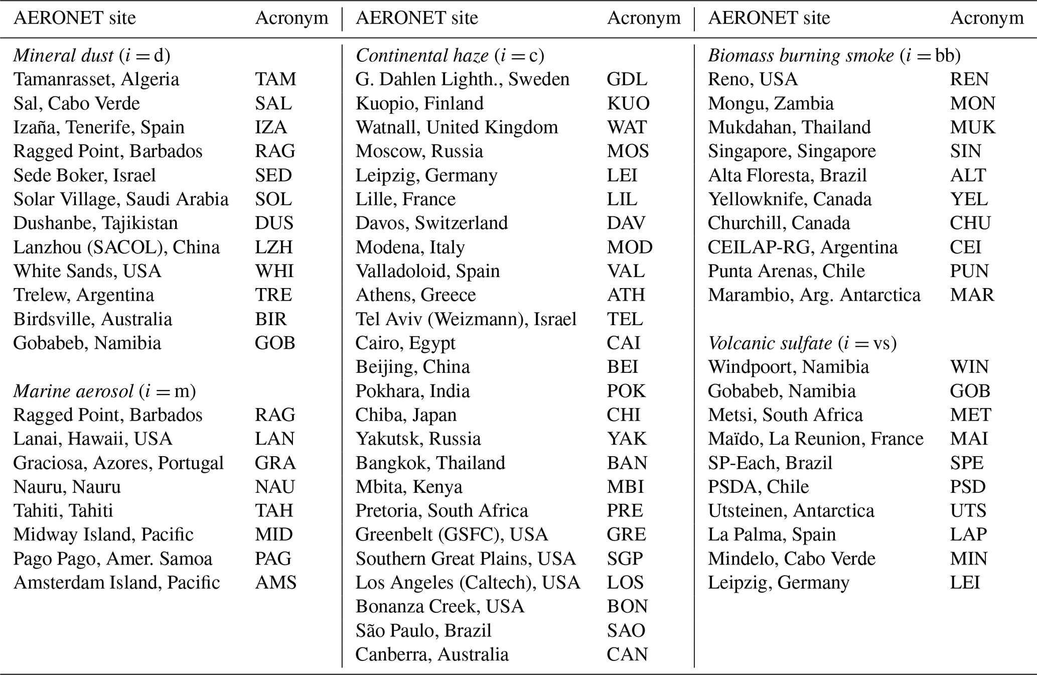
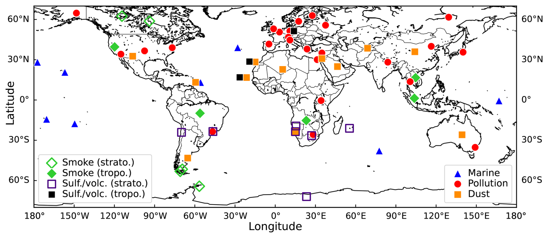
Figure 2 Distribution of the selected 62 AERONET stations over the globe. For the determination of marine, continental (urban, rural), and dust conversion factors, we used the observations at 8 marine AERONET stations (blue triangles), at 25 continental sites (red circles), at 12 stations close to deserts (orange squares). Observations of strong wildfire smoke events at 10 stations (green diamonds) and of pronounced volcanic sulfate layers at 10 sites (black squares) allowed the retrieval of wildfire smoke and volcanic sulfate conversion factors.

3.2 Selected AERONET stations

Table 3 and Fig. 2 provide an overview of all selected 62 AERONET stations used in our statistical data analysis. We selected 12 AERONET stations in or close to desert regions to be able to determine conversion factors for pure desert dust conditions (i = d). Similarly, we selected 8 stations on islands in the Pacific, Indian, and Atlantic Ocean with long-term observations of more than 10 years in order to derive representative marine-aerosol conversion factors (i = m). In the case of continental anthropogenic pollution (i = c), we selected 25 AERONET stations to cover remote (background), rural, and urban conditions on different continents.

In the case of wildfire smoke observations (i = bb), we used the stations, data sets, and data filtering options in this POLIPHON update effort as selected in Ansmann et al. (2021). However, this time, we excluded the observations at the Table Mountain station in California. The impact of urban haze from the Los Angeles region is always high and does not allow a trustworthy retrieval of pure smoke conversion factors. In Ansmann et al. (2021), conversion factors for 532 nm were presented, only. Now we repeated all computations for all four wavelengths, i.e., for 355, 532, 911, and 1064 nm, and applied, for the first time, also a weighted linear regressions analysis (York et al., 2004) to the wildfire smoke observations.

In the case of the stratospheric sulfate conversion factors for fresh volcanic aerosol (from the Hunga Tonga-Hunga Ha'apai volcanic eruption in mid-January 2022, in the following simply denoted as Hunga Tonga eruption), we used the same observations (stations, measurement days, observation times) as presented in Figs. 3 and 4 in Boichu et al. (2023). These stations are Maïdo on La Reunion, France, Windpoort and Gobabeb in Namibia, Metsi in South Africa, SP-EACH at São Paulo, Brazil, and PSDA, Chile, located in the Antofagasta region in northern Chile. The observations in late-January 2022 are characteristic for fresh sulfate (effective radius around 300 to 500 nm) with a low impact of sedimentation and removal of large particles. The volcanic sulfate particles formed a well defined accumulation mode (similar to the one of UTLS wildfire smoke).

To obtain conversion factors for aged Hunga Tonga sulfate aerosol, one year after the eruption, we used the observations at the Antarctic AERONET site of Utsteinen (72° S, 23.3° E, 1400 m above sea level, 160 km away from the Southern Ocean). The 500 nm AOT is close to 0.02 at unperturbed atmospheric conditions over the Antarctic stations so that any further AOT contribution, e.g., from the stratosphere, is visible in the data. The effective radius was 160 nm for these unperturbed aerosol conditions in January 2022. One year later, in January 2023, under the full influence of Hunga Tonga aerosol, the AOT increased to 0.04–0.05 and the effective radius of the pronounced accumulation mode caused by the volcanic sulfate aerosol was around 250 nm. These Utsteinen AOT observations were found to be in good agreement with our lidar observations at the German Antarctic Neumayer station (about 500 km west of the Utsteinen site) during the first months of 2023. The profile data showed 532 nm AOTs of 0.02–0.025 for the height range from the tropopause up to 20 km. According to the AERONET observations discussed by Boichu et al. (2023), the 500 nm AOT caused by the volcanic aerosol was of the order of 0.3–0.5 and the effective radius of the well-defined accumulation mode was close to 400 nm in January 2022.

We used the opportunity to analyze volcanic sulfate layers in the lower troposphere. Respective observations could be recently realized after the eruptions of the Cumbre Vieja volcano on La Palma in the autumn of 2021 (Córdoba-Jabonero et al., 2023; Gebauer et al., 2024). We included observations at Leipzig after the eruption of the Icelandic Eyjafjallajökull volcano in April 2010 in this study (Ansmann et al., 2011).

3.3 Downloaded AERONET products and aerosol-type-dependent data filtering

The data downloaded from the AERONET data base (AERONET, 2026; Sinyuk et al., 2020) for each station in Table 3 are listed in Table 4. The version-3-inversion data files contain AOT values for 440, 675, 870 and 1020 nm, separately for fine-mode and coarse-mode aerosol, and the corresponding particle size distribution for each individual observational data set. Furthermore, the volume and surface-area concentrations, separately for fine-mode and coarse-mode fractions, are available. These products are sufficient to calculate all conversion factors for 532 and 911 nm. From interpolations between neighboring AOT values by using respective Ångström exponents, we obtained the 532 and 911 nm total (fine-mode and coarse-mode), fine-mode, and coarse-mode AOTs. In, principle, the version-3-inversion data files with all the AOT information for 440, 675, 870 and 1020 nm can also be used to extrapolate to 355 and 1064 nm in order to create fine-mode, coarse-mode and total AOT data sets for 355 and 1064 nm.

Table 4 AERONET level 2.0 data downloaded for each selected marine, dust, and continental-haze AERONET station in Table 3. These AERONET products are required to derive the sets of conversion factors for all four lidar/ceilometer wavelengths of 355, 532, 911, and 1064 nm. In the case of tropospheric and stratospheric volcanic sulfate layers and stratospheric wildfire smoke, level 1.5 AOT data and corresponding inversion products are used.

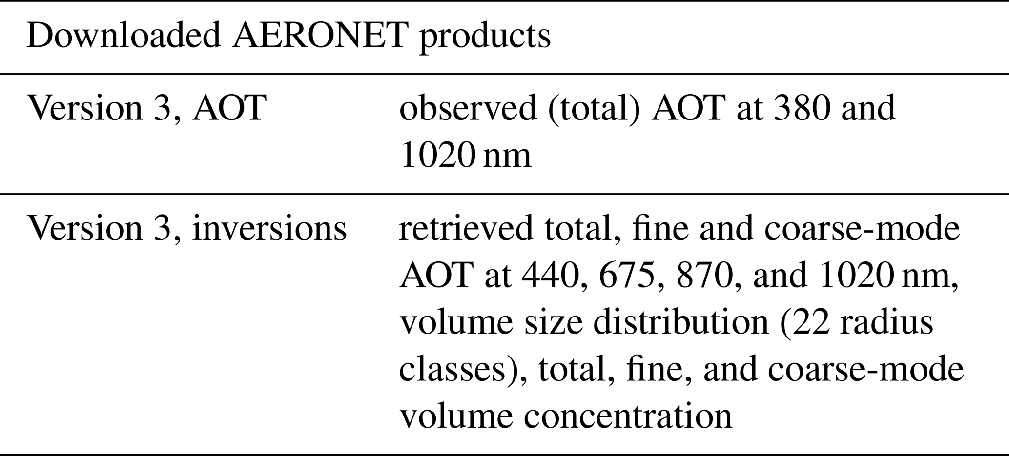
However, the specific absorbing and scattering features of mineral dust and wildfire smoke in the 355–532 nm wavelength range cannot be accurately reproduced by simple extrapolation of the 355 nm AOT from the version-3-inversion AOTs for the 440–1020 nm wavelength spectrum. Therefore, we used the directly observed 380 and 440 nm AOTs (Version 3, AOT data in Table 4) to obtain the 355 nm (total) AOT by extrapolation. Afterwards, we selected those 355 nm AOT values that were temporally close to the observations used to retrieve the version-3 inversion products. Analogously, we determined and selected the respective 1064 nm AOT values from directly measured 870 and 1020 nm AOTs. In the next step, we computed the coarse-mode AOTs at 355 and 1064 nm via extrapolation by using the coarse-mode AOT information in the version-3-inversion data files (covering the wavelength range from 440 to 1020 nm). Finally, we calculated the difference between the total and the coarse-mode AOTs to obtain the fine mode AOTs at 355 and 1064 nm. Internal checks and comparison between the total, fine-mode, and coarse-mode AOTs from 355 to 1064 nm indicated the consistency between all optical data.

Most conversion factors were computed by using total AOT and respective total (fine + coarse-mode) size distribution data. However, the wildfire smoke and volcanic sulfate conversion factors were determined by using the fine-mode AOTs and the respective microphysical properties computed from the fine-mode part of the size distribution, only. More details to this aspect can be found in Ansmann et al. (2021). The fine-mode data in the AERONET data base cover the full size distributions (well-formed, monomodal accumulation mode) of wildfire smoke and volcanic sulfate particles.

It should be emphasized that the fine-mode AOT is almost equal to the total AOT in the case of wildfire and volcanic-sulfate-dominated observations. This means that the computation of the 355 and 1064 nm coarse-mode AOTs and subsequent subtraction from the total AOTs do not introduce a significant bias in the fine-mode AOT data required to derive the wildfire smoke and volcanic sulfate conversion factors.

Note that in the case of all AERONET observations with a strong impact of UTLS aerosols on the measured AOT, only level 1.5 AERONET data are available. These UTLS-aerosol-dominated observations are completely removed and are not part of the level 2.0 data base. Similarly, many of the level 1.5 data are removed in the case of lower tropospheric volcanic sulfate layers. Level 1.5 data are cloud-screened but not further checked for instrumental biases. Level-2.0 data are available after regular inspection and calibration of the photometers at AERONET topical centers and recalculation of the level 1.5 data by using, e.g., updated filter transmission functions. Thus, we decided to use level 1.5 data in all analyses of tropospheric and stratospheric volcanic sulfate layers and in the analysis of UTLS smoke layers. Level 2.0 data were used in the case of lower tropospheric smoke data, only.

After setting up proper data fields of the total, fine-mode, and coarse-mode AOT and related microphysical inversion products, we can step forward towards the regression analyses. Well defined data sets for pure marine, pure dust, and pure continental haze conditions are needed in the correlation studies to obtain the aerosol-type-dependent conversion factors. We applied the filter options as defined in Table 5 to identify and select all pure marine observations conducted at the 8 marine AERONET stations, the pure dust cases over the 12 desert AERONET stations, and the continental-haze-dominated measurements over the 25 urban and rural continental AERONET sites defined in Table 3. For the sake of completness, the regression analysis considers dust fine-mode AOTs and the respective dust fine-mode column volume concentrations and, respectively, dust coarse-mode AOTs and dust coarse-mode column volume concentrations to obtain the dust fine-mode and coarse-mode volume conversion factors c_v,df and c_v,dc.

Ansmann et al. (2021)Ansmann et al. (2021)

Table 5 Data filtering and selection options in the POLIPHON conversion-factor retrievals. In the case of continental, marine and dust aerosol, only AERONET observations that fulfill the listed conditions for the Ångström exponent (AE) and the 532 nm AOT conditions are considered in the statistical analysis. The wildfire-smoke filter options are the same as in Ansmann et al. (2021). Manually selected observations are used in the case of volcanic sulfate layers as described in Sect. 3.2.

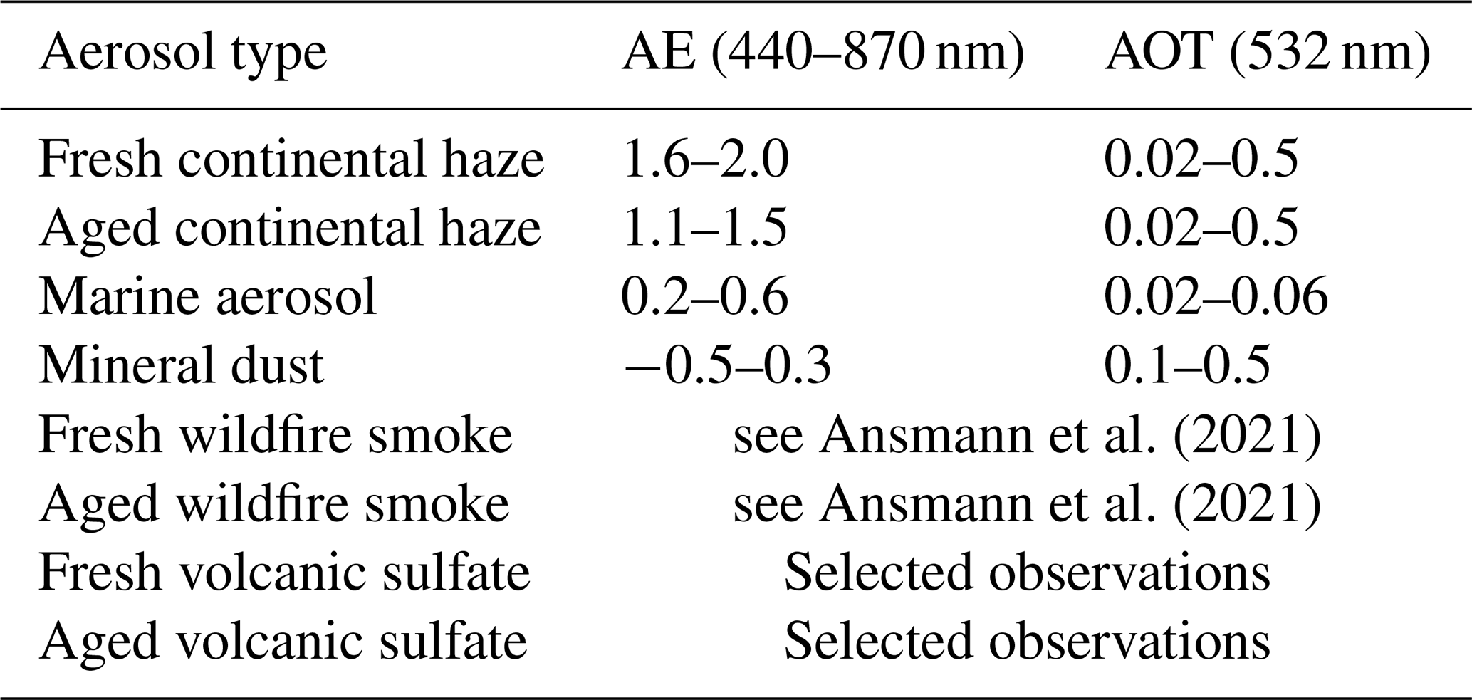
Note that we considered 532 nm AOT < 0.5, only, in the dust-related analysis to avoid any bias introduced by potentially incorrect AERONET observations that may occur in rather dense aerosols along the sunphotometer observational path. Such conditions may especially be given during measurements shortly after sunrise and shortly before sun set (Ansmann et al., 2019b). Fortunately, there are several AERONET stations that showed low bias at greater AOTs > 0.5, and in these cases we did not find a strong hint that we have a bias when we ignore all dust situations with AOT > 0.5. On the other hand, the majority of dust events around the globe show AOTs < 0.5 at 500–550 nm so that our conversion factors, presented here, are applicable to all these dust scenarios. In more than 80 % of cases out of all observations at AERONET stations close to dust source regions, 500 nm AOT < 0.5 was found.

The Ångström exponent AE for the 440–870 nm wavelength range was used to distinguish the different basic aerosol types. High AE values of 1.6–2.0 indicate urban haze with a large fraction of freshly produced small particles. Lower AE values of 1.1–1.5 indicate aged aerosol ensembles, in most cases a mixture of anthropogenic pollution and soil, road, and industrial dust. Very low and low AE values of < 0.3 (mineral dust) and from 0.2–0.6 (marine aerosol) are caused by coarse-mode dominated particle ensembles. Because AE values of 0.2–0.6 can also occur during dust events, we used the 532 nm AOT to distinguish dust from marine observations. Only dust cases with a 532 nm AOT exceeding 0.1 were considered in the statistical regression analyses. Marine AOTs are usually well below 0.07. A clear discrimination option to distinguish dust-dominated and marine-aerosol-dominated observations is important for AERONET stations on the islands of Tenerife (Izaña), Cabo Verde, and Barbados (Ragged Point). The filtering conditions for wildfire smoke were discussed in Ansmann et al. (2021) and in the foregoing section for volcanic sulfate aerosol.

Table 6 Data analysis concept to obtain the POLIPHON conversion factors (column 1, dry, required in Table 2) from AERONET observations at ambient conditions (index: amb, columns 3 and 4) in the case of marine (m), dust (d), and continental (c) pollution particles. The applied linear regression analysis with the x_i,j and y_i,j data fields (described in Appendix A) then lead to the factors for ambient humidity conditions (column 2, ambient). These derived conversion factors are interpreted as the required dry-aerosol conversion factors assuming a mean RH during the AERONET observations as given in column 5 (RH). Column 6 (Unit) shows the units of the individual conversion factors. All individual regression analysis procedures listed in the table are separately repeated for each individual extinction coefficient data set ${\mathit{\sigma }}_{i,\text{amb},j}\left(\mathrm{355}\mathrm{nm}\right)$, ${\mathit{\sigma }}_{i,\text{amb},j}\left(\mathrm{532}\mathrm{nm}\right)$, ${\mathit{\sigma }}_{i,\text{amb},j}\left(\mathrm{911}\mathrm{nm}\right)$, and ${\mathit{\sigma }}_{i,\text{amb},j}\left(\mathrm{1064}\mathrm{nm}\right)$.

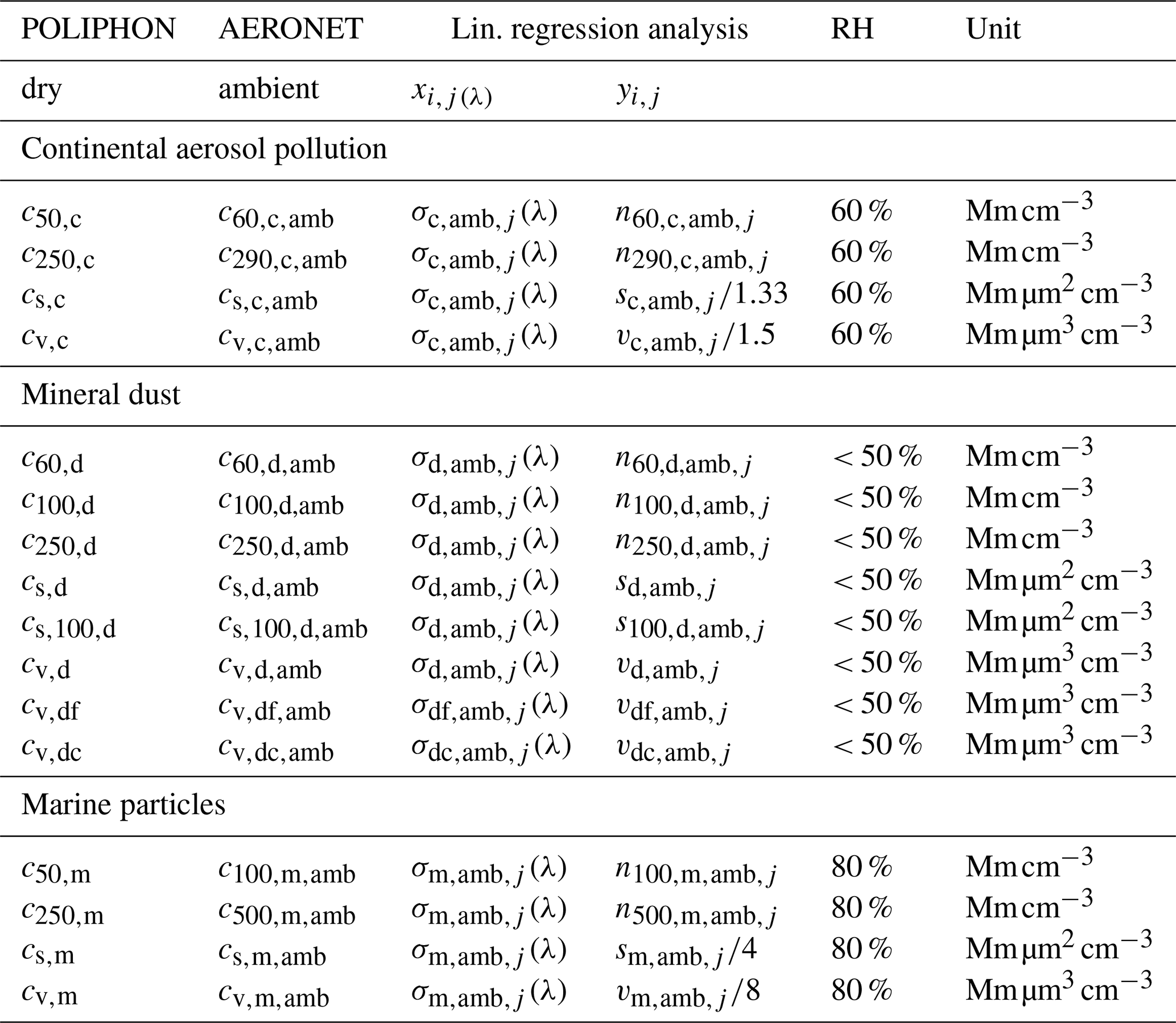
3.4 From observations at ambient humidity conditions to dry-aerosol conversion factors

One of the most important aspects to be considered in the regression analyses is the need for dry-aerosol conversion factors in Table 2. However, the AERONET observations are conducted at ambient humidity conditions. As a result of water uptake, hygroscopic particles in the air are larger at RH of 80 % than at RH of 40 % when they are dry or almost dry. This increase in particle size must be taken into account in the statistical analyses. The strategy to obtain the dry-aerosol conversion factors from AERONET aerosol data observed at ambient RH conditions is explained in Table 6. In order to be in line with the notation in Table 2 and the general lidar nomenclature (particle extinction coefficient instead of AOT, number, surface, volume, and mass concentration instead of column values of these quantities), we divided all AERONET AOTs and column microphyscial products by a typical vertical atmospheric length scale (aerosol layer depth) of 1000 m, and proceed with these data sets within the linear regression studies. This change is considered in Table 6.

The goal is to derive those conversion factors (in column 2 in Table 6) from the regression analysis with x_i,j(λ) and y_i,j data sets for swollen aerosol particles (in columns 3 and 4) that can be interpreted as conversion factors (in column 1) needed to solve the equations in Table 2. More details to this topic can be found in Mamouri and Ansmann (2016, 2017).

We may explain our basic data analysis concept by the following examples for continental haze: $c_{\mathrm{60},\mathrm{c},\text{amb}}$ is the obtained conversion factor when applying the linear regression analysis to all data pairs ${\mathit{\sigma }}_{\mathrm{c},\text{amb},j}$ and $n_{\mathrm{60},\mathrm{c},\text{amb},j}$ (with observational running index j from 1 to N_obs). $n_{\mathrm{60},\mathrm{c},\text{amb},j}$ considers all particles with radius > 60 nm. We assume a typical RH of 60 % during the AERONET observations. The continental pollution particles shrink by about 15 %–20 % when the relative humidity decreases to 40 % (dry conditions). This means that $n_{\mathrm{60},\mathrm{c},\text{amb},j}$ is approximately equal to $n_{\mathrm{50},\mathrm{c},\text{dry},j}$ and represents the particle number concentrations considering all dry particles with radius > 50 nm.

As indicated in Table 6, over polluted continents with a strong fraction of hygroscopic sulfate particles, a small water uptake effects has to be generally considered. Even when the photometer observations over rural and urban AERONET sites are conducted at sunny conditions, an RH of 60 % as an RH average value for entire continental planetary boundary layer PBL must be considered. Most of the aerosol (usually more than 80 %–90 % of the tropospheric aerosol content) resides in the boundary layer over the polluted continents. As mentioned, at these slightly enhanced humidity conditions the particle radius is about a factor of 1.15 ± 0.05 larger than the dry-particle radius at RH < 40 % (Skupin et al., 2016).

We assume an even higher marine PBL RH value of 80 % over the island stations during the observations of marine aerosols so that we expect a particle radius increase by roughly a factor of 2.0 according to an extinction enhancement factor of 3.7 at 532 nm as observed by Haarig et al. (2017) when RH increased from dry conditions with RH = 40 % to humid conditions with RH = 80 %. Such very high enhancement factors close to 4 could be measured in pure marine air over Barbados during the winter season in the absence of any continental influence from Africa, South and Central America.

Water vapor effects are neglected in the case of desert dust observations, RH < 50 % is assumed during the sunny AERONET observations at the AERONET stations close to or in deserts. As in the case of desert dust, we also assume dry conditions (RH < 50 %) during wildfire smoke and volcanic sulfate observations. Dry conditions generally prevailed in the upper troposphere and lower stratosphere and were probably also given in most cases of AERONET observations of smoke in the lowest 5 km of the troposphere over the AERONET stations in or close to fire regions. In the case of the few observations of lower tropospheric volcanic sulfate layers, we also assumed dry conditions in the regression analysis for a better comparison of all determined tropospheric and stratospheric sulfate conversion factors.

As described in detail in Mamouri and Ansmann (2016, 2017), the respective dry-aerosol surface area concentrations and volume concentrations for continental aerosol pollution (at RH = 40 %) are a factor of 1.33 and 1.5, respectively, lower than the ambient-condition (RH=60 %) surface area and volume concentrations in the case that the particle radius decreases by a factor of 1.15. Similarly, the dry aerosol surface area and volume values are smaller by a factor of 4 and 8 than the observed ones, respectively, when the particle radius shrinks by a factor of 2. These factors are considered in Table 6 (columns 2, 3, and 4).

In the case of the conversion factor, used to obtain particle number concentrations, we used a different way to consider the water uptake effect. As shown in Table 6, we simply interpret the computed values of $n_{\mathrm{60},\mathrm{c},\text{amb},j}$ and $n_{\mathrm{290},\mathrm{c},\text{amb},j}$ as $n_{\mathrm{50},\mathrm{c},\text{dry},j}$ and $n_{\mathrm{250},\mathrm{c},\text{dry},j}$, respectively, when assuming a particle radius reduction by a factor of 1.15. Similarly for marine aerosol, we assume that the observed values $n_{\mathrm{100},\mathrm{m},\text{amb},j}$ and $n_{\mathrm{500},\mathrm{m},\text{amb},j}$ are representative for the respective dry-aerosol values $n_{\mathrm{50},\mathrm{m},\text{dry},j}$ and $n_{\mathrm{250},\mathrm{m},\text{dry},j}$, respectively, when the particle radius is reduced by a factor of 2.

3.5 Correction of humidity effects in actual lidar observation

If nearby radiosonde observations are available so that a precise knowledge of the RH profile is given one can, in principle, transfers the continental extinction coefficient measured with lidar at a given RH level to extinction coefficients at 60 % in the retrieval of urban and rural continental aerosol microphysical properties, to the extinction coefficient at 80 % in the retrieval of the microphysical properties of marine particles, and to extinction values for 40 % in the retrieval of dust, smoke and volcanic sulfate microphysical properties before applying the POLIPHON conversion factors as given in Table 6 (column 1). The RH-related transfer of the extinction coefficient can be done following the Hänel parameterization (Hänel, 1976; Skupin et al., 2016; Haarig et al., 2017, 2025). If radiosonde observations are not available one may use modeled RH profiles. However, these profiles have to be generally handled with caution. Especially during conditions with cloud developments, modeled RH fields may not reflect properly the true RH conditions during the lidar observations. In such complicated cases, we recommend to leave out any humidity correction.

As a further remark, we recommend to avoid the application of the POLIPHON method in cases of lidar observations just below the base of cloud layer, i.e., where RH is of the order > 90 % so that strong water uptake by the particles causes large backscatter and extinction coefficients. The use of these large backscatter and extinction coefficients in the POLIPHON computations may lead strong biases (overestimation) in the estimates of the microphysical properties because of the large and not well known RH-controlled impact of water uptake effects. We recommend to use only POLIPHON products in aerosol–cloud-interaction studies for heights at least 500 m below the observed cloud base heights (Jimenez et al., 2020).

It is also worth noting that spaceborne lidar applications rely on trustworthy aerosol observations in the lateral vicinity of clouds layers in aerosol–cloud interaction studies. However, enhanced hygroscopic growth at high relative humidity can increase aerosol scattering by up to 80 % near these cloud boundaries (Twohy et al., 2009). Therefore, studies considering POLIPHON applications to spaceborne lidar data should exclude aerosol profiles in direct contact with a cloudy column, i.e., aerosol profiles measured within an area of approximately 5 km around the cloud field of interest.

4 Regression analysis results

The results of the statistical analysis of four contrasting AERONET data sets are discussed in Sect. 4.1 to introduce the basic products of the correlation studies and explain the variability in the results and what statistical quantity best represents the required specific conversion factor. In Sect. 4.2, the conversion factor sets for all individual marine, dust, and continental-pollution AERONET stations are presented and the variability in these conversion factors is discussed. In Sect. 4.3, mean values of all determined conversions factors are presented as a function of aerosol type and wavelength. All in all, 1488 individual regression analyses were performed to obtain 96 different conversion factors (for the 5 aerosol types and 4 wavelengths).

4.1 Case studies

Table 7 shows the results of the regression analysis applied to four contrasting AERONET data sets. Desert dust observations (IZA, Izana, Tenerife), a marine case (AMS, Amsterdam Islands) and observations at two urban AERONET stations (BEI, Beijing, China; PRE, Pretoria, South Africa) were used in the correlation studies. As outlined in Appendix A, the applied least-squares estimation method of fitting the best straight line to data points x_i,j and y_i,j delivers the slope b_i and the intercept a_i. In our AERONET-based statistical data analysis, slope b_i is a good proxy for the conversion factor c_i, describing the relationship between the extinction coefficient (x_i) and the microphyscial product (y_i). Physically, the most reasonable solution for b_i is given when a_i≈0, so that the microphysical values are close to zero when the particle extinction coefficient is close to zero. However, due to the scatter in the y_i,j values, mostly caused by AERONET retrieval uncertainties, the intercept a_i is larger or lower than 0. Table 7 shows a few examples of solution sets for the intercept a_i±δa_i and slope b_i±δb_i in the case of the linear regression analysis with $x_{\mathrm{d},j}={\mathit{\sigma }}_{\mathrm{d},\text{amb},j}$ at 532 nm and $y_{\mathrm{d},j}=n_{\mathrm{100},\mathrm{d},\text{amb},j}$ (IZA, dust observations, c_100,d retrieval). The Amsterdam Island example uses $x_{\mathrm{m},j}={\mathit{\sigma }}_{\mathrm{m},\text{amb},j}$ at 532 nm and $y_{\mathrm{m},j}=n_{\mathrm{100},\mathrm{m},\text{amb},j}$ (Amsterdam Island, AMS, marine conditions, c_50,m retrieval). The urban examples are based on the regression analysis with $x_{\mathrm{c},j}={\mathit{\sigma }}_{\mathrm{c},\text{amb},j}$ at 532 nm and $y_{\mathrm{c},j}=n_{\mathrm{60},\mathrm{c},\text{amb},j}$ (BEI, urban haze, AE range: 1.1–1.5, PRE, urban haze, AE range: 1.6–2.0, c_50,c retrieval).

Table 7 Solutions of the linear regression analysis for intercept a_i (in cm⁻³) and slope b_i (in Mm cm⁻³), and the ratio $\stackrel{\mathrm{‾}}{y_i}/\stackrel{\mathrm{‾}}{x_i}$ (in Mm cm⁻³) by using ${\mathit{\sigma }}_{i,\text{amb},j}\left(\mathrm{532}\mathrm{nm}\right)$ as x_i,j and $n_{\mathrm{100},\mathrm{d},\text{amb},j}$ (IZA), $n_{\mathrm{100},\mathrm{m},\text{amb},j}$ (AMS), $n_{\mathrm{60},\mathrm{c},\text{amb},j}$ (BEI), and $n_{\mathrm{60},\mathrm{c},\text{amb},j}$ (PRE) as y_i,j. N_obs is the number of observed x_i,j and y_i,j data pairs considered in the individual regression analyses. R² is the coefficient of determination. The computation of the different quantities, uncertainties δa and δb, and the coefficient of determination R² is explained in Appendix A. The correlation studies are performed to obtain the dry-particle POLIPHON conversion factors c_100,d (IZA), c_50,m (AMS), c_50,c (BEI, AE:1.1–1.5) and c_50cy (PRE, AE:1.6–2.0) as required in Table 2. The $\stackrel{\mathrm{‾}}{y_i}/\stackrel{\mathrm{‾}}{x_i}$ values are interpreted as the optimum solution for the sought conversion factors.

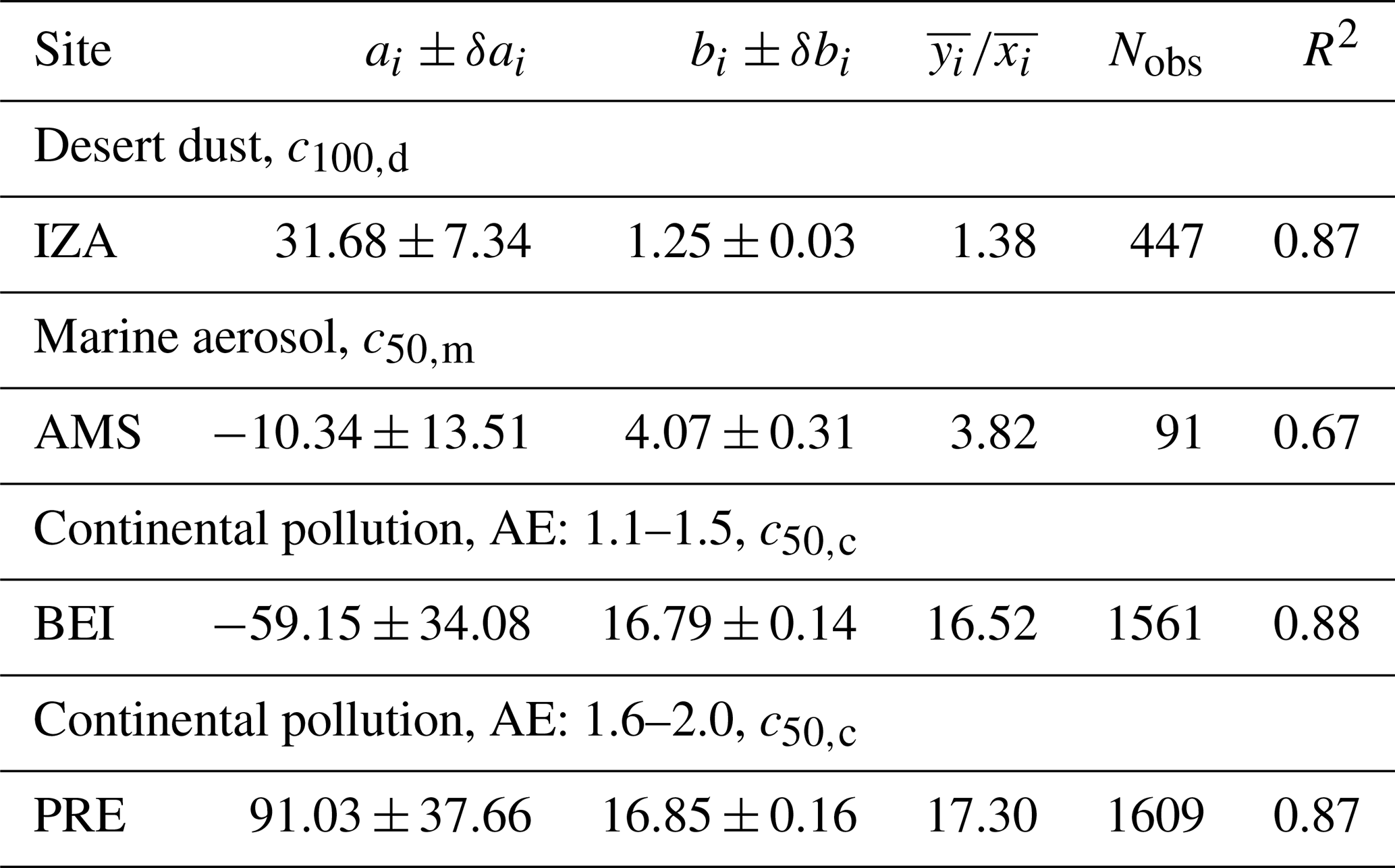
As can be seen, the intercept value a_i can have a noticeable impact on the solution for b_i. According to Eq. (A1), the slope b_i is equal to $\stackrel{\mathrm{‾}}{y_i}/\stackrel{\mathrm{‾}}{x_i}$ when the intercept is a_i=0. We see that b_i is smaller than this ideal b_i (for a_i=0) when a_i is positive, and vice versa, b_i is larger than the ideal b_i when a_i is negative. In most cases, it was found that a_i had only a minor impact on the determination of b_i, so that b_i was close to $\stackrel{\mathrm{‾}}{y_i}/\stackrel{\mathrm{‾}}{x_i}$ (within about 5 % around $\stackrel{\mathrm{‾}}{y_i}/\stackrel{\mathrm{‾}}{x_i}$) as is the case in Table 7 for the Beijing and Pretoria data.

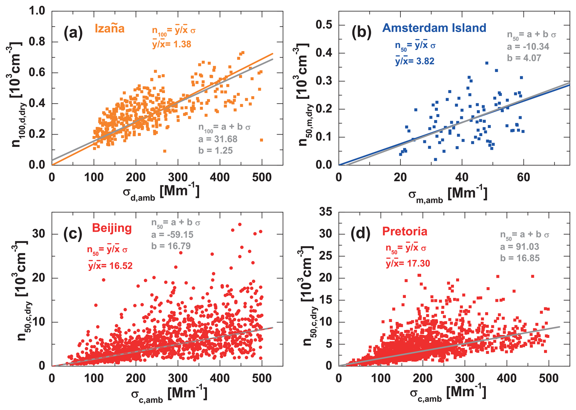
Figure 3 Number concentration $n_{\mathrm{100},\mathrm{d},\text{dry}}$ (a, Izaña), $n_{\mathrm{50},\mathrm{m},\text{dry}}$ (b, Amsterdam Island), $n_{\mathrm{50},\mathrm{c},\text{dry}}$ (c, Beijing, AE range from 1.1–1.5) and Pretoria (d, for the AE range from 1.6–2.0) versus respective particle extinction coefficient σ_i,amb(532 nm). The regression lines are obtained from the weighted linear regression analysis applied to 447 (a), 91 (b), 1561 (c), and 1609 (d) individual AERONET observations performed at the four sites. Table 7 contains the regression products a, b, and $\stackrel{\mathrm{‾}}{y}/\stackrel{\mathrm{‾}}{x}$ which are used to compute the gray and colored regression lines, respectively.

In Fig. 3, the available data and obtained regression products are shown. The different, but similar regression lines corroborate that the use of the $\stackrel{\mathrm{‾}}{y_i}/\stackrel{\mathrm{‾}}{x_i}$ values as conversion factors is fully justified. Note, that the shown c_50,i and c_100,d retrievals are the most critical ones compared to retrievals of the conversion factors used to estimate n₂₅₀, surface area and volume concentrations. In Fig. 3, the statistical analysis is based on strongly scattered data with a considerable fraction of unwanted outliers. The data are less noisy in the case of the other conversion factors (Mamouri and Ansmann, 2016, 2017; Ansmann et al., 2019b).

In the following tables in Sects. 4.2 and 4.3, we use the values for $\stackrel{\mathrm{‾}}{y_i}/\stackrel{\mathrm{‾}}{x_i}$ with the weighted mean values $\stackrel{\mathrm{‾}}{x_i}$ and $\stackrel{\mathrm{‾}}{y_i}$ according to Eqs. (A2) and (A3), respectively, as the conversion factors and interpret them as the dry-aerosol conversion factors that are needed in the main POLIPHON Table 2 to obtain the microphysical properties $n_{\mathrm{50},i,\text{dry}}$, $n_{\mathrm{100},i,\text{dry}}$, $n_{\mathrm{250},i,\text{dry}}$, s_i,dry, and v_i,dry.

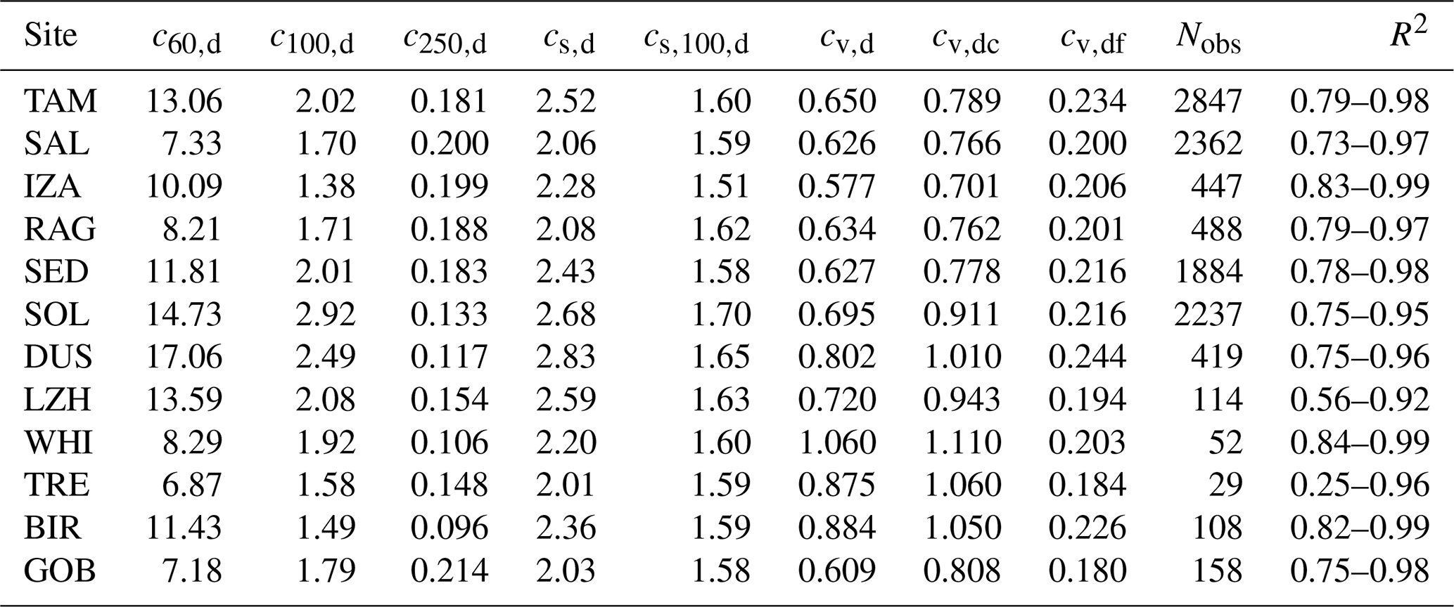
Table 8 532 nm POLIPHON conversion factors for the dust aerosol type (i = d), derived from dust observations at 12 AERONET stations. The full names of the stations are given in Table 3. Units of the conversion factors are given in Table 6. N_obs is the number of observed x_j and y_j data pairs considered in the individual regression analysis. R² is the coefficient of determination. Detailed explanations to the conversion factors are provided in Sects. 2.4, 3.1, and 3.4.

4.2 Station-by-station analysis

Tables 8–11 show the products of the regression analyses for all AERONET stations. The 532 nm conversion factors are listed. Table 8 contains the dust conversion factors obtained from the analysis of the selected 12 dust AERONET stations. The marine conversion factors in Table 9 are obtained from the regression studies with the observations at the 8 selected marine stations. Tables 10 and 11 show all conversion factors for anthropogenic haze derived from the selected 25 selected continental rural and urban AERONET stations. As already mentioned, N_obs in the four tables is the number of used x_i,j and y_i,j data pairs in the correlation studies and R² is the coefficient of determination and indicates the uncertainty in the obtained results. The lowest R² values are usually obtained in the c_50,i and c_60,d regression studies. The highest R² values are usually obtained for c_s,i and c_v,i.

Table 9 Same as Table 8, except for the marine aerosol type (i = m). The 532 nm POLIPHON conversion factors are derived from observations at 8 marine AERONET sites (island stations, far away from continents, see Fig. 2).

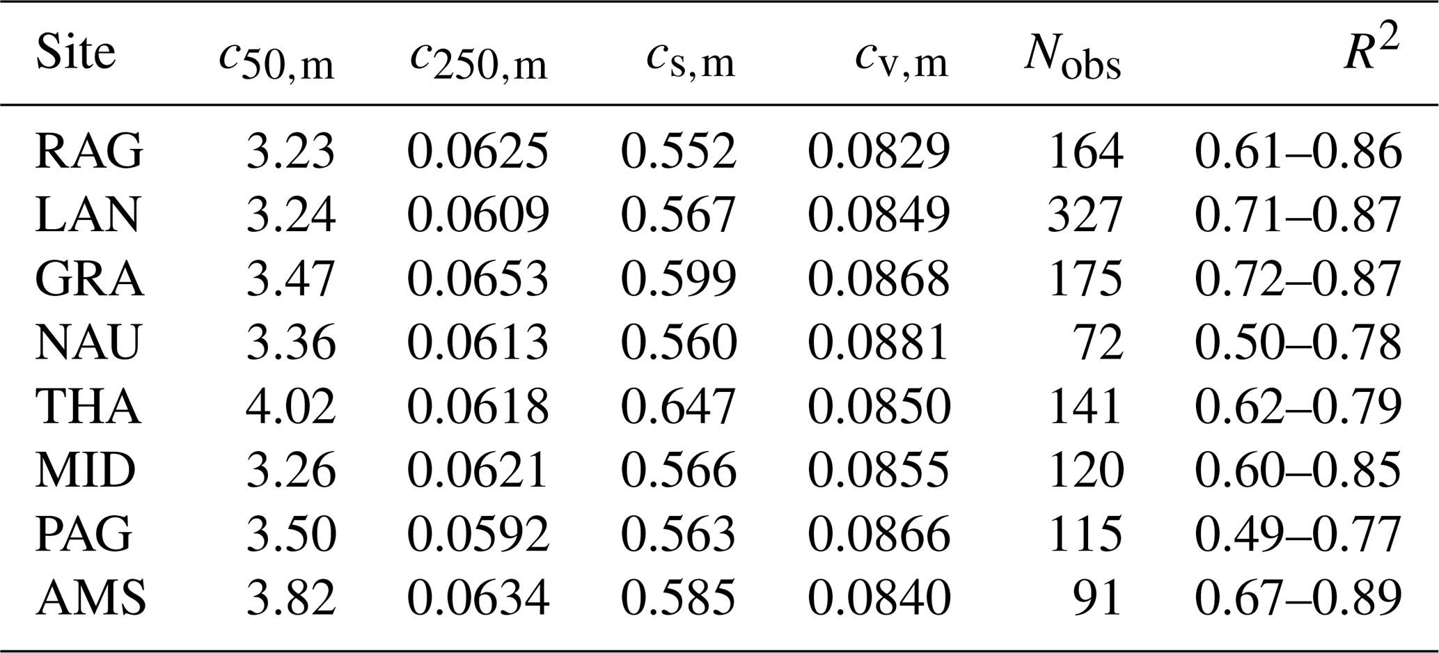
Table 10 Same as Table 8, except for the continental-pollution aerosol type (i = c). The 532 nm POLIPHON conversion factors are derived from observations at 25 continental, urban and rural AERONET stations (see Fig. 2). Only 532 nm AOT observations (and corresponding microphysical products) are considered in the statistical analysis showing AE values from 1.1–1.5. These relatively low AE values indicate aged continental pollution particles and the impact of local dust. Further filtering options are given in Table 5.

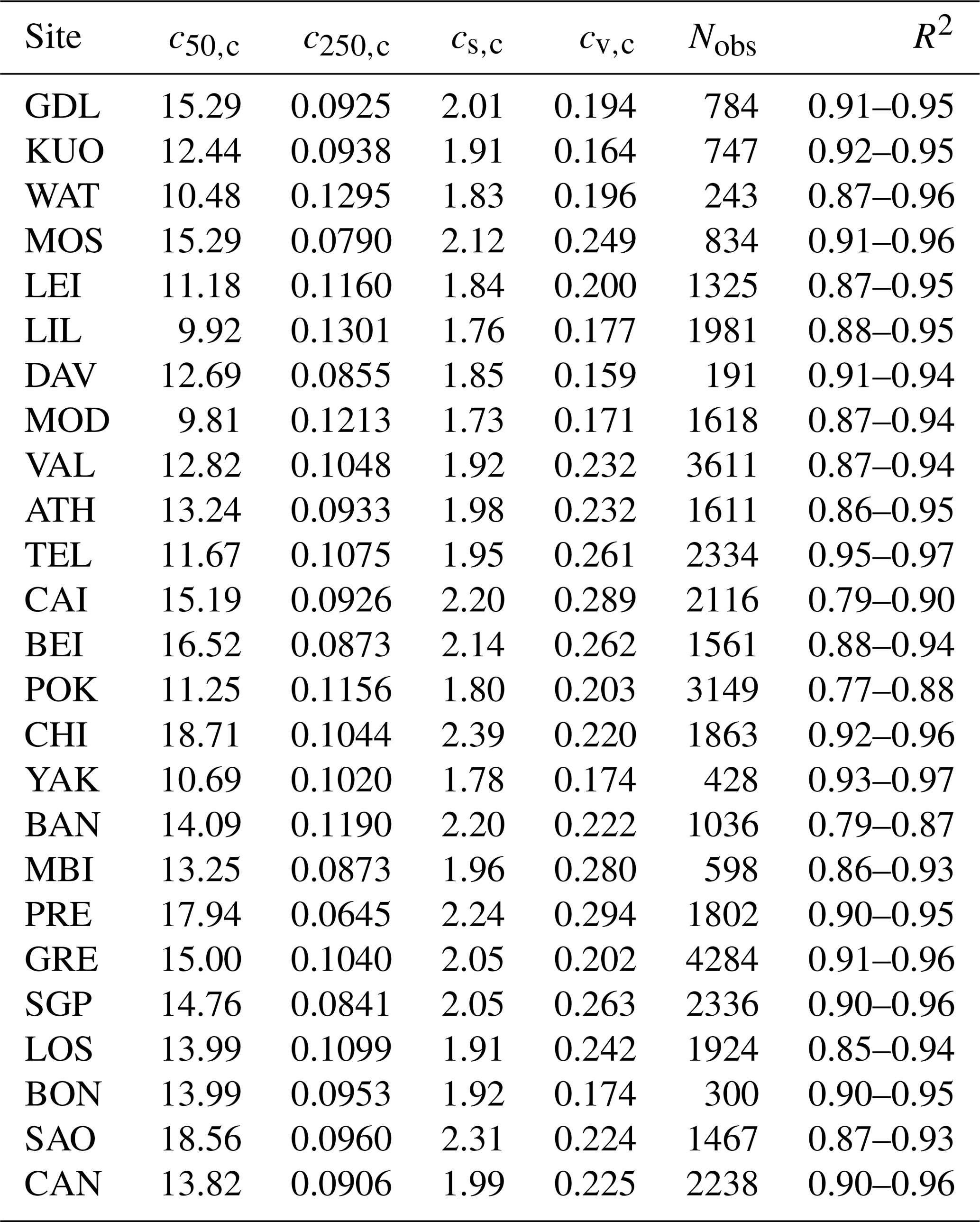
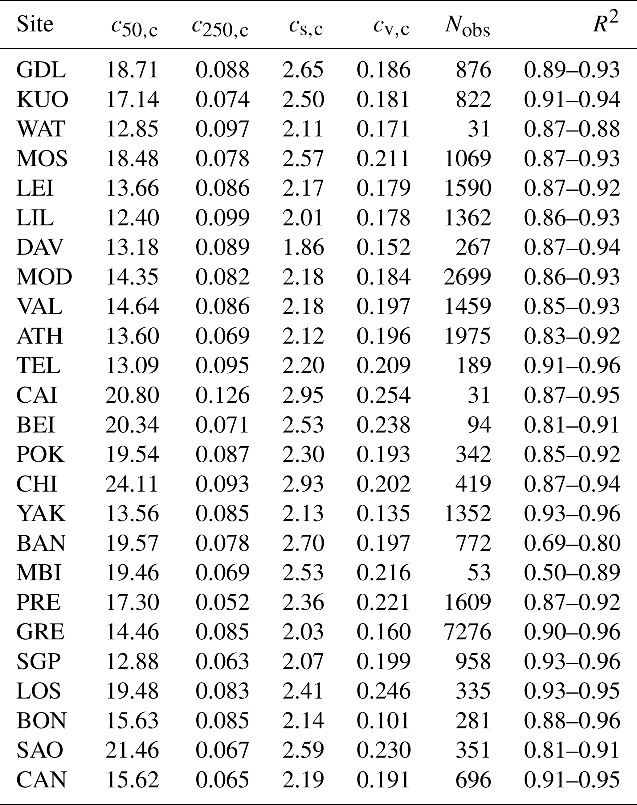
Table 11 Same as Table 10, except for the continental-pollution aerosol type and considering AERONET observations showing AE values from 1.6–2.0. These high AE values indicate fresh pollution, i.e., smaller particles.

The station-by-station results in the four tables provide an impression of the variability in the obtained conversion factors for the three main aerosol types. The reasons for the variability are varying ambient humidity conditions during the observations, varying aerosol conditions, especially regarding the size distributions of the observed aerosol mixtures over the polluted continents, and uncertainties in the AERONET inversion products (y_i,j values).

Fairly similar conversion factor sets were obtained for the different stations in the case of pure dust (Table 8) and pure marine observations (Table 9). A less homogeneous picture was obtained from the AERONET observations of anthropogenic pollution (Tables 10 and 11). As a new aspect, we distinguish between continental anthropogenic pollution for the two different AE ranges to better cover conditions with aged and fresh anthropogenic pollution and situations with urban haze and pollution conditions preferably occurring in rural regions. AE of 1.6–2.0 indicates the dominance of freshly produced, relatively small anthropogenic particles whereas AE from 1.1–1.5 suggests a considerable impact of larger particles, i.e., of aged anthropogenic particles including mixtures of fine-mode pollution and coarse-mode particles such as road, soil, and industrial dust. In winter, residential heating including wood burning (Malollari et al., 2025) contributes to the haze over the continents while during other seasons, bioaerosol (pollen, spores) and biological material from agricultural and harvesting activities may dominate the coarse-mode fraction. In the original study (Mamouri and Ansmann, 2016), we only considered the conversion factors for the AE 1.6–2.0 range, but especially at rural sites, the conversion factors for the 1.1–1.5 AE range may be more appropriate to estimate CCN concentrations. The comparison of the conversion factors in Tables 10 and 11 reveals that the conversion factors are typically different by 10 %–20 %. The conversion factors c_50,c and c_s are lower, and thus n_50,c and s_c are lower for a given extinction coefficient, in the case of aerosols mixtures showing AE from 1.1–1.5 compared to the respective values for AE from 1.6–2.0. The opposite is the case for the c_250,c and c_v,c conversion factors.

Regional differences in the dust conversion factors as discussed in Ansmann et al. (2019b) may exist, but seem to be small. The most robust AERONET inversion product is the surface area concentration for dust particles with radius > 100 nm, and thus the most trustworthy conversion factor is $c_{\mathrm{s},\mathrm{100},\mathrm{d}}$ in Table 8. Gerasopoulos et al. (2007) stated that the uncertainty in the particle size distribution is large for the particles with radius < 100 nm and > 7 µm (> 50 %) and small (10 %) for particles with radius from 100 nm to 7 µm. As can be seen, all values of $c_{\mathrm{s},\mathrm{100},\mathrm{d}}$ for different desert stations (WHI, TAM, TRE, BIR, GOB) are in the range from 1.58 and 1.60 Mm µm² cm⁻³. Regional differences are not visible. The variability of the other conversion factors in Table 8, e.g., of c_v,d of 0.65 Mm µm³ cm⁻³ (TAM), 1.06 Mm µm³ cm⁻³ (WHI), 0.88 Mm µm³ cm⁻³ (TRE), 0.88 Mm µm³ cm⁻³ (BIR), and 0.61 Mm µm³ cm⁻³ (GOB) may be the result of a combination of uncertainties in the inversion products and local aerosol characteristics. Regional aspects cannot be fully excluded when discussing conversion factors for AERONET stations close to deserts in Australia, South and North America, Africa, and Asia, but the regional impact is weak.

Figures 4 and 5 show the impact of the conversion factor variability on the retrieval of the CCN and dry-aerosol mass concentrations in the case of marine, dusty, and haze conditions. The particle extinction coefficient at 532 nm is set to 100 Mm⁻¹ and converted into the shown CCN and dry-mass concentration values. As can be seen, a rather low variability in the POLIPHON results and thus in the respective conversion factors is observed in the case of marine particles. Rather homogeneous conditions obviously prevail over the AERONET island stations during pure marine conditions as defined in Table 5. A similar conclusion can be drawn in the case of desert dust. A stronger variability is observed for anthropogenic haze conditions. One needs to take a 50 % uncertainty always into account in CCN estimations.

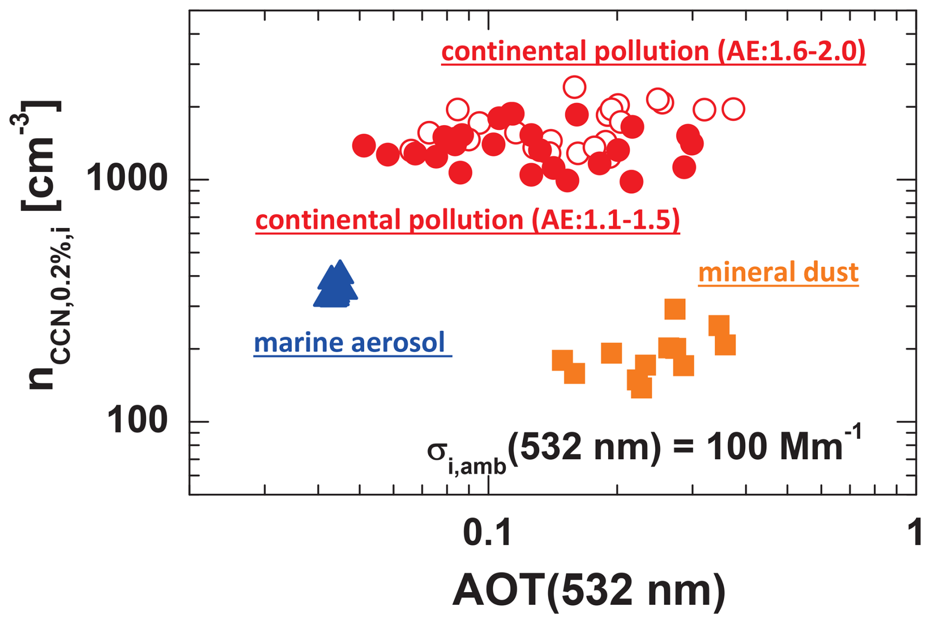
Figure 4 Impact of individual, station-by-station conversion factors on the estimated CCN number concentration. A 532 nm particle extinction coefficient σ_i,amb(532 nm) = 100 Mm⁻¹ is converted into $n_{\text{CCN},\mathrm{0.2}\mathit{\%},i}$ values by using the equations in Table 2. Eight individual marine conversion factors c_50,m are used to compute n_CCN,m (blue triangles), 12 dust conversion factors c_100,d are applied to obtain n_CCN,d (orange squares), and 25 continental-pollution conversion factors c_50,c, derived from AERONET observation with AE from 1.1–1.5 (solid red circles) and from AERONET observations with AE from 1.6–2.0 (open red circles) are used to obtain n_CCN,c. To better visualize the impact of the individual, station-by-station conversion factors, the CCN solutions are shown as a function of the station-mean 532 nm AOT, which is computed from all observations at a given AERONET site that were included in the respective individual conversion-factor determination.

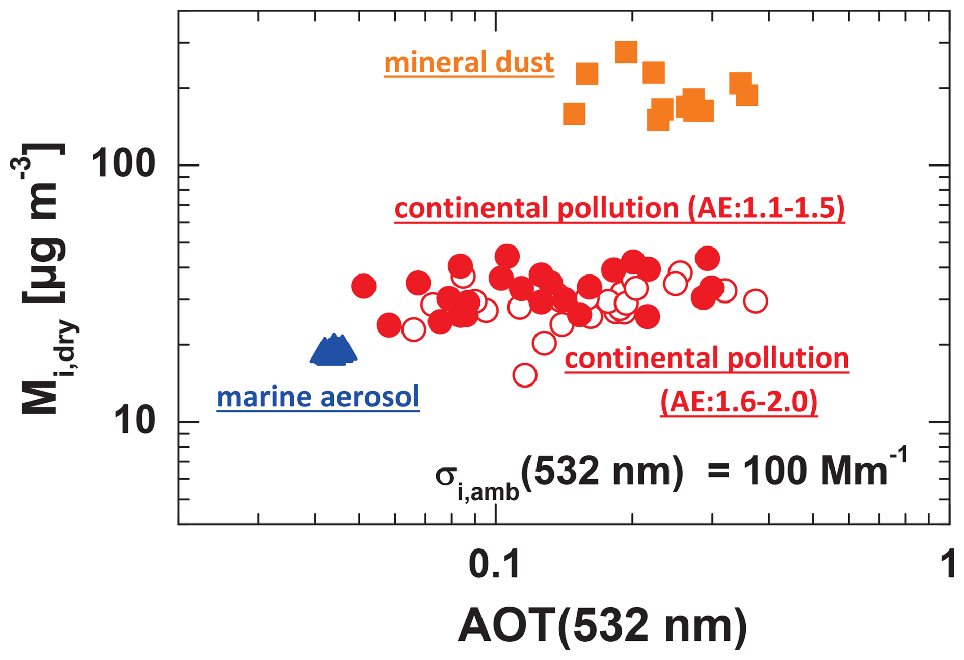
Figure 5 Same as Fig. 4, except for the computation of the dry-particle mass concentration from 532 nm particle extinction coefficient σ_i,amb(532 nm) = 100 Mm⁻¹. The conversion factors c_v,i and particle densities of 2.16 (dry marine), 1.5 (sulfate), and 2.6 g cm⁻³ (dust) are used.

One aspect is left to be discussed here. Papetta et al. (2026) compared balloon-borne in situ observations of dust volume concentrations and dust extinction coefficients with respective products from AERONET observations at Cabo Verde in September 2022 and concluded that AERONET-based volume conversion factors may be up to 50 % lower than the true conversion factors in the case of dust events with a strong fraction of very large to giant dust particles (with particle radius exceeding 15 µm). The AERONET inversion algorithm only considers dust particles with radius < 15 µm so that the derived volume concentrations are wrong if a significant amount of large to giant particles are present. However, these special cases that may occur after strong dust storms over desert regions or during dust devil events (Ansmann et al., 2009) seem to be rare. Except the lidar observation during the dust devils events in southeastern Morocco, close to Saharan dust sources in the summer of 2006, we never observed cases in which large to giant particles dominated the lidar observations. Only a few lidar observations are reported in the literature (Burton et al., 2015; Hu et al., 2020), that indicated the occurrence of a strong fraction of large to giant dust particles so that the use of the AERONET conversion factors presented here may lead to an underestimation of the dust mass concentration as Papetta et al. (2026) suggest.

4.3 Analysis summary: Mean conversion factors for 5 aerosol types and 4 wavelengths

Mean values for all conversion factors, for the five aerosol types, and the four wavelengths are presented in Tables 12–15. All station-by-station values, listed in Tables 8–11 were averaged, separately for each conversion factor and aerosol type, to obtain the mean 532 nm conversion factors for the three fundamental aerosol types (marine, dust, continental pollution). In the same way, the data sets of conversion factors for 355, 911, and 1064 nm were processed. The results are shown in Tables 12 and 13. The statistical analyses applied to the wildfire smoke and volcanic sulfate observations lead to the conversion factors given in Tables 14 and 15.

Table 12 Dust conversion factors (dust cf) for the conversion of σ_d,amb(355 nm) and σ_d,amb(532 nm) into respective dust particle number, surface area, and volume concentrations. These POLIPHON conversion factors can be used in Table 2. The individual, station-by-station conversion factors of the 12 AERONET dust sites were averaged and the respective mean values and one standard deviations are listed.

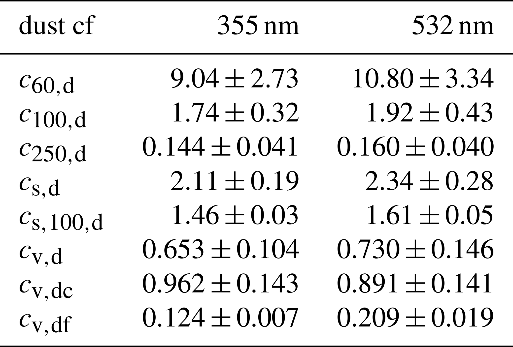
Table 13 Mean values of POLIPHON conversion factors for the 4 aerosol lidar and ceilometer wavelengths. The conversion factors for the three main aerosol types, derived from observations at 8 marine, 12 dust, and 25 continental-pollution AERONET stations, are averaged. The mean values and corresponding one standard deviations in this table are shown in Fig. 6. The units of the conversion factors are given in Table 6.

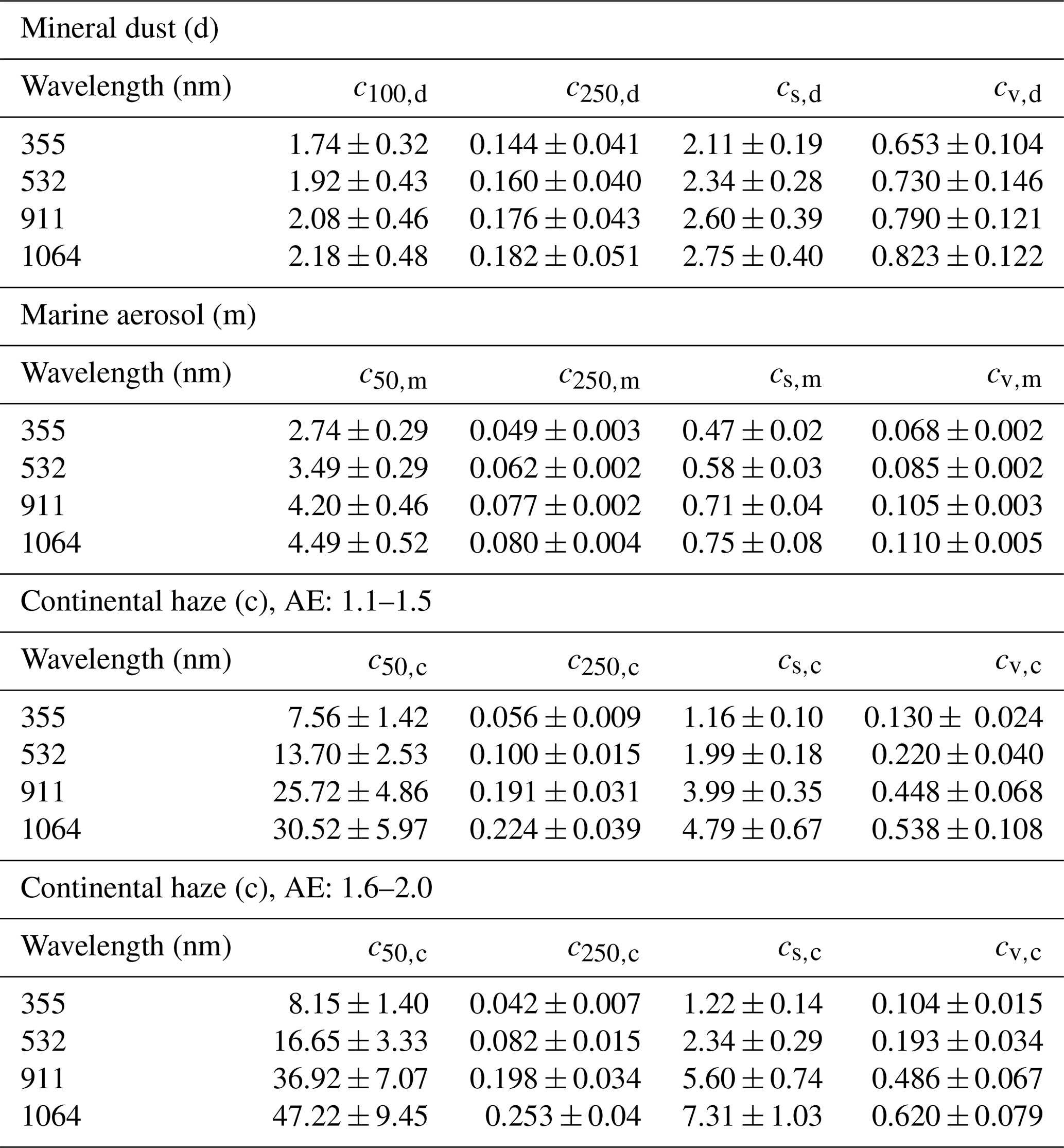
Table 14 Same as Table 13, except for wildfire smoke (BB smoke). The mean values and corresponding SD values are shown in Fig. 7 as well.

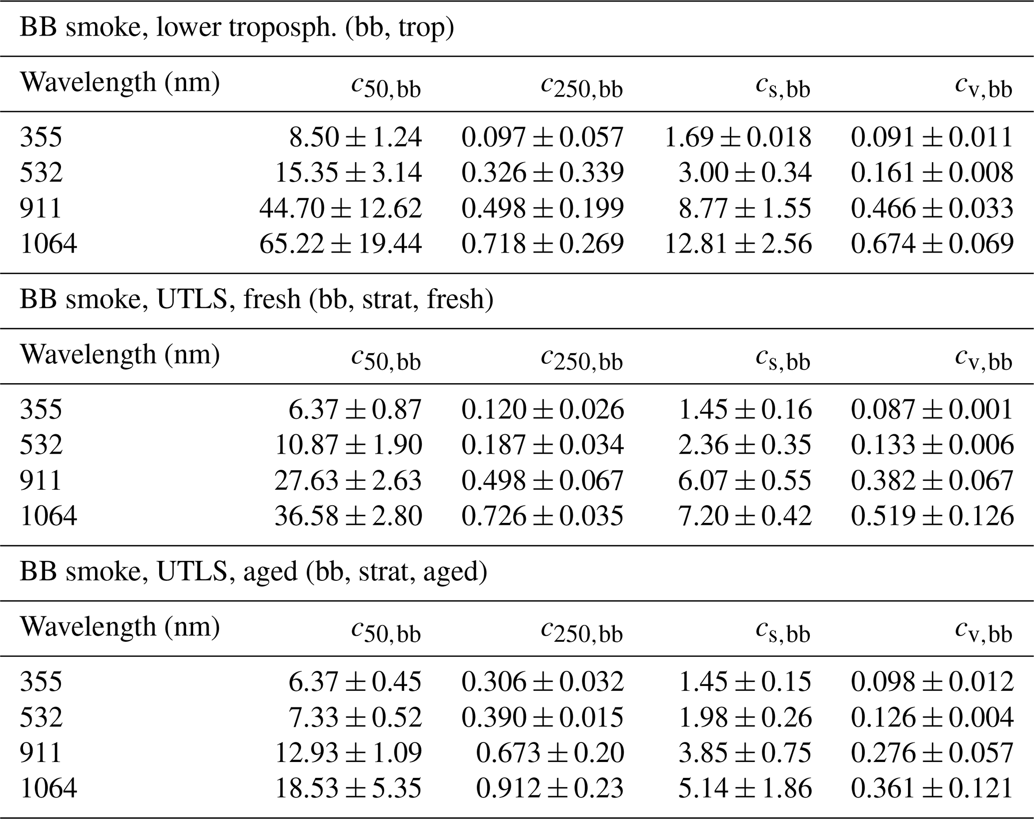
Table 15 Same as Table 13, except for volcanic sulfate aerosol (vs). The mean values and corresponding SD values are shown in Fig. 7 as well.

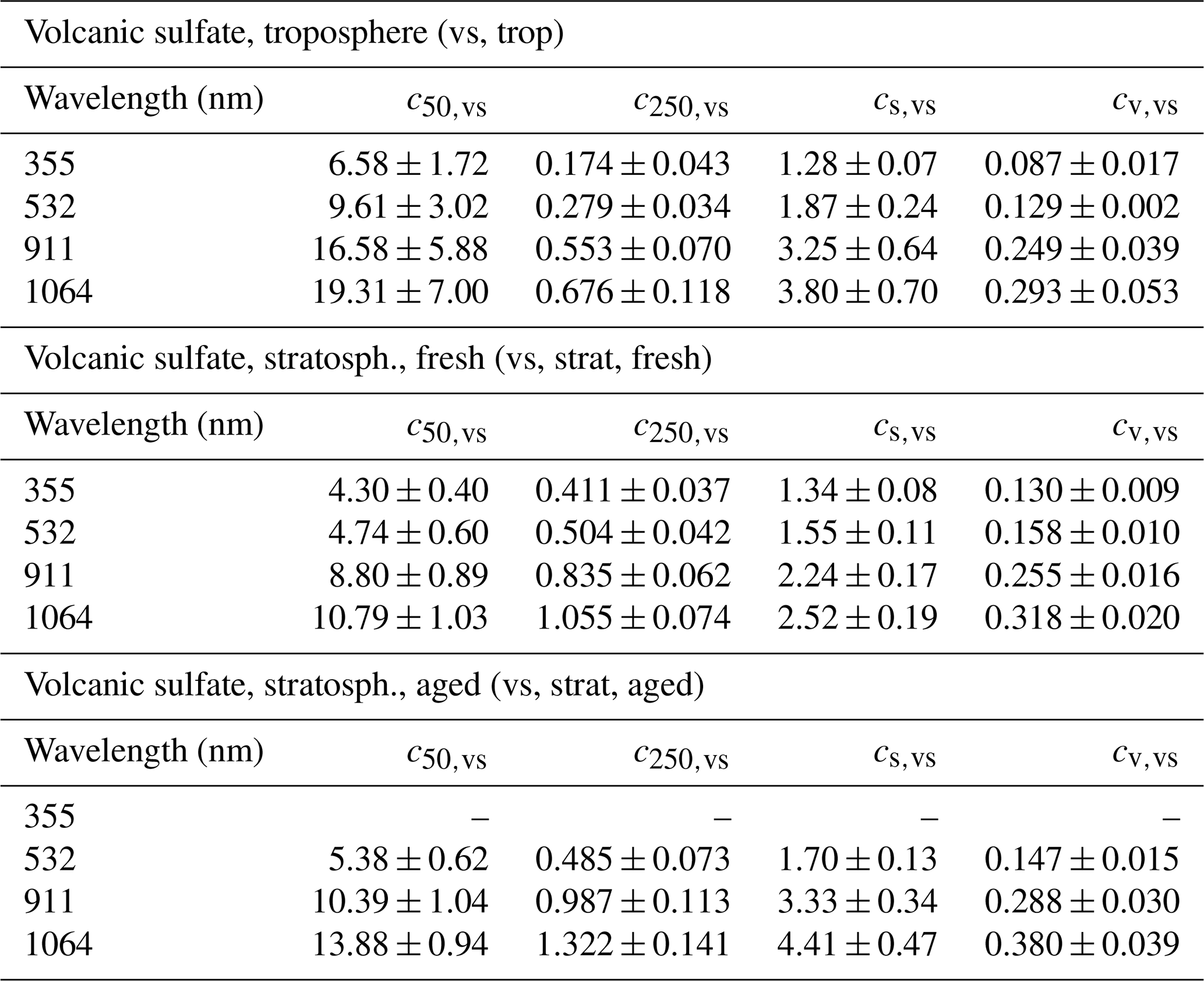
Table 12 is explicitly presented as support to the dust observations around the globe with CALIOP and ACDL (532 nm laser wavelength) and ALADIN and ATLID (355 nm wavelength). Mean values and standard deviations (SD) are listed. To combine the long-term aerosol observations, performed since 2006, in terms of microphysical properties in a coherent way, an internally consistent conversion factor set as given in Table 12 is required.

Table 13 contains mean values of the four fundamental conversion factors c_50,i, c_250,i, c_s,i, and c_v,i for the three basic aerosol types and the four wavelengths. In principle, one can use the individual conversion factor data in Tables 8–11 in cases with lidar and ceilometer observations close to one of the considered stations. However, when comparing ceilometer or lidar network data (on a continental scale), it is recommended to use the mean conversion factors given in Table 13.

The same AERONET data analysis procedure as described above and presented in Tables 8–13 for the marine, dust, and pollution aerosol types, was applied to the wildfire smoke and volcanic sulfate observations. The finally obtained mean values are shown in Tables 14 and 15. The tropospheric smoke conversion factors were obtained from the analysis of the AERONET observations at Reno, Mongu, Mukdahan, Singapore, and Alta Floresta (listed in Table 3). More details are given in Ansmann et al. (2021). Fresh UTLS wildfire smoke conversion factors were calculated from the stratospheric smoke observations at Yellowknife and Churchill in Canada in August 2017. The measurements of Australian smoke more than 10 000 km east of the smoke sources in Australia, originating from strong bush fires in December 2019 and January 2020, at the AERONET stations in South America (Punta Arenas, CEILAP RG) and Antarctica (Marambio) were used to determine the conversion factors for aged UTLS wildfire smoke (Ansmann et al., 2021).

The observations at the 6 AERONET stations Windpoort, Gobabeb, Metsi, Maido, SP-Each, and PSDA, listed in Table 3 and suggested by Boichu et al. (2023), were used to determine conversion factors for fresh stratospheric volcanic sulfate layers. These layers were observed during the first two weeks after the eruption of the Hunga Tonga volcano. Large AOTs of 0.3–0.5 and large sulfate particles with a particle effective radius of around 400 nm prevailed to that time.

The Antarctic observations at the AERONET station of Utsteinen in January 2023 (1 year after the eruption) were used to determine the conversion factors for size distributions of aged stratospheric volcanic sulfate layers, affected by sedimentation and tropopause-fold-related removal processes (Ansmann et al., 1997). The effective radius of the remaining volcanic sulfate particles was reduced to values around 250 nm after one year of long-range transport and the stratospheric contribution to the overall 532 nm AOT was about 0.02, in good agreement with our Antarctic lidar observations in the first half of 2023 (Radenz et al., 2024). For 355 nm, no useful results could be obtained. The main reason is that the determination of the stratospheric 355 nm AOT via extrapolation by using the observed 380 and 440 nm AOTs was not reliable.

We used the opportunity of the eruption of the Cumbre Vieja volcano (1120 $\mathrm{m}\mathrm{a}.\mathrm{s}.\mathrm{l}.$) on La Palma, Canary Islands, Spain, in September 2021 (Córdoba-Jabonero et al., 2023; Gebauer et al., 2024) to retrieve conversion factors for volcanic sulfate layers in the lower troposphere. The AERONET station La Palma (at 630 $\mathrm{m}\mathrm{a}.\mathrm{s}.\mathrm{l}.$ height) is located 18 km south of the volcano. We analyzed several observations conducted from 26 September to 22 October 2021. Volcanic sulfate aerosol could also be measured at the AERONET station of Mindelo, Cabo Verde, about 1500 km southwest of La Palma, from 23–27 September 2021. The air masses need 3 d to reach Mindelo. We added a few observations of a fully developed volcanic sulfate layer in the lower troposphere over Leipzig, 5–6 d after the emission of SO₂ plumes by the Eyjafjallajökull volcano on Iceland which erupted on 14 April 2010 (Ansmann et al., 2011).

The mean values and standard deviations considering all observations from all three stations are given in Table 15. For the individual stations we obtained the following regression results for c_50,vs (Mm cm⁻³), c_250,vs (Mm cm⁻³), c_s,vs (Mm µm² cm⁻³), and c_v,vs (Mm µm³ cm⁻³): 12.9, 0.25, 2.13, 0.13 for La Palma, 7.1, 0.31, 1.65, 0.13 for Mindelo, and 8.7, 0.28, 1.83, 0.13 for Leipzig.

These conversion factors for lower tropospheric volcanic sulfate layers have to be handled with caution. Most trustworthy are the values for free tropospheric aerosol conditions (above about 650 m height) at La Palma. However, these conversion factors for rather fresh sulfate plumes may not be representative for aged sulfate layers. For the Mindelo AERONET station (1500 km southwest of La Palma, 3 d of air mass transport in September 2021) (Gebauer et al., 2024), the volcanic aerosol was mixed with marine particles. The 532 nm AOT was 0.5 to 0.9 on 23–25 September, and around 0.3 on 26 and 27 September 2021 and thus much larger than the 532 nm AOT of about 0.05 for undisturbed marine conditions. The Mindelo conversion factors (not corrected for any potential water uptake effect) fit well into the scheme of conversion factors for rather fresh sulfate plumes (La Palma) and the aged volcanic sulfate layers in the stratosphere as listed in Table 15. In the case of the Leipzig conversion factors, the role of urban haze and the respective condensations of sulfuric acid on the existing anthropopgenic particles is not known as well as the impact of not corrected water uptake effects. On both analyzed days (19–20 April 2010), sunny and dry conditions prevailed over central Europe. The observed 532 nm AOT over Leipzig was 0.4–0.75 and thus much larger than the typically observed 532 nm AOT of 0.1. All in all, the values in Table 15 may be taken for conversion of lidar and ceilometer observations in the lower troposphere by assuming a general uncertainty of 50 %.

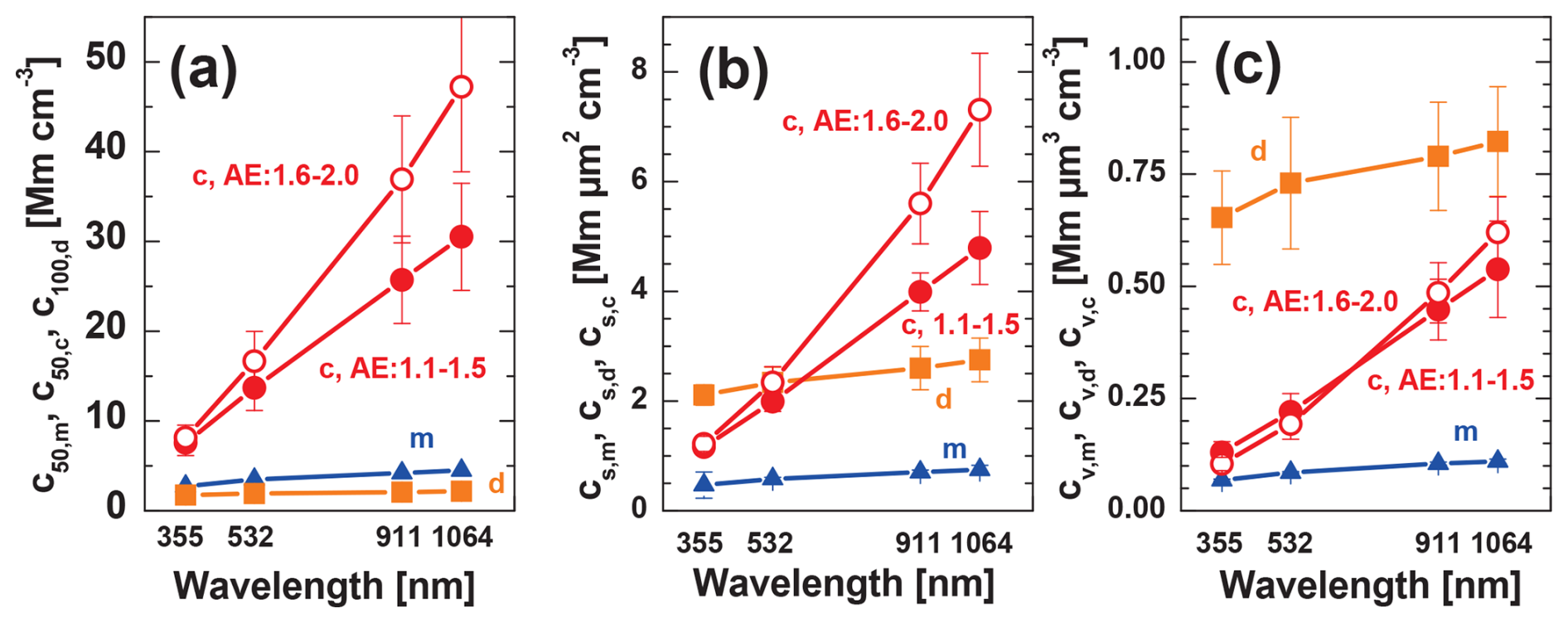
Figure 6 POLIPHON conversion factors (mean and SD) as a function of wavelength. (a) c_50,m (blue), c_50,c (solid red circles for AE from 1.1–1.5), open red circles for AE from 1.6–2.0), and c_100,d (orange), (b) same as (a) except for c_s,i with i = m, c, and d , and (c) same as (b) except for c_v,i. The values in Table 13 are shown together with SD (error bars).

Figure 7 Same as Fig. 6, except for wildfire smoke (bb) and volcanic sulfate layers (vs). The values in Tables 14 and 15 are shown together with SD (error bars).

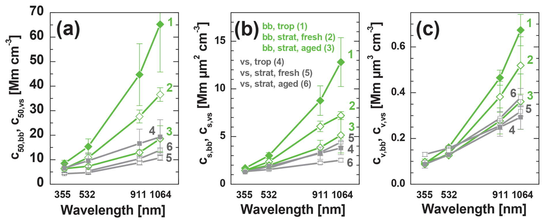
Figures 6 and 7 provide an overview of the wavelength dependence of the mean conversion factors c_50,i, c_s,i, and c_v,i. The mean values in the Tables 12, 14, and 15 are shown together with the respective SD (one standard deviation). The vertical SD bars thus indicate the variability in the station-by-station conversion factors. In the case of the Utsteinen conversion factors, we use the uncertainty δb_vs in the slope b_vs obtained from the regression analysis to indicate the potential uncertainty in the conversion factors.

The wavelength dependence of the conversion factors is directly related to the wavelength dependence of the particle extinction coefficient (or AERONET AOT) of the different aerosol types. The wavelength dependence is low for coarse-mode-dominated dust and marine aerosols and high for fine-mode-dominated aerosol ensembles (haze, smoke, and volcanic sulfate aerosols).

4.4 Discussion: Comparison of updated (2026) with previous (2016, 2019) conversion factors and conversion factors from alternative retrievals

The most critical conversion, associated with potentially large uncertainties, is the conversion of extinction coefficients into CCN concentrations. However, this approach is an important analysis tool in field studies of aerosol–cloud interaction. In this final subsection, we provide comparisons of the updated extinction-to-CCN conversion method with our previous conversion approach (Mamouri and Ansmann, 2016; Ansmann et al., 2019b) and with a few similar alternative conversion efforts (Choudhury et al., 2022; Lenhardt et al., 2023).

In Figs. 8 and 9, we show the relationship between the estimated dry-state particle number concentration $n_{\mathrm{50},\mathrm{m},\text{dry}}$, $n_{\mathrm{50},\mathrm{c},\text{dry}}$, and $n_{\mathrm{100},\mathrm{d},\text{dry}}$ (used as proxy for n_CCN) and the respective 532 nm particle extinction coefficient σ_m,amb, σ_c,amb, and σ_d,amb, measured at ambient humidity conditions with RH of typically 60 % (continental aerosol), 80 % (marine environment) and < 50 % (dry desert conditions). The number-vs-extinction relationships are defined by the linear equation $n_{\text{dry}}=c\times {\mathit{\sigma }}_{\text{amb}}$ with conversion factor c in Figs. 8 and 9 in the case of the A26 curves (this study) and the C22 curves in Fig. 9 (Choudhury et al., 2022). In the case of our previous studies (Mamouri and Ansmann, 2016; Ansmann et al., 2019b) as well as in the study of H25 (He et al., 2025a), the estimation is based on the relationship $n_{\text{dry}}=c\times {\mathit{\sigma }}_{\text{amb}}^{x_{\mathrm{p}}}$ with the additional extinction exponent x_p as input. x_p results from the linear regression with data in the log scale and is typically between 0.75 and 1.

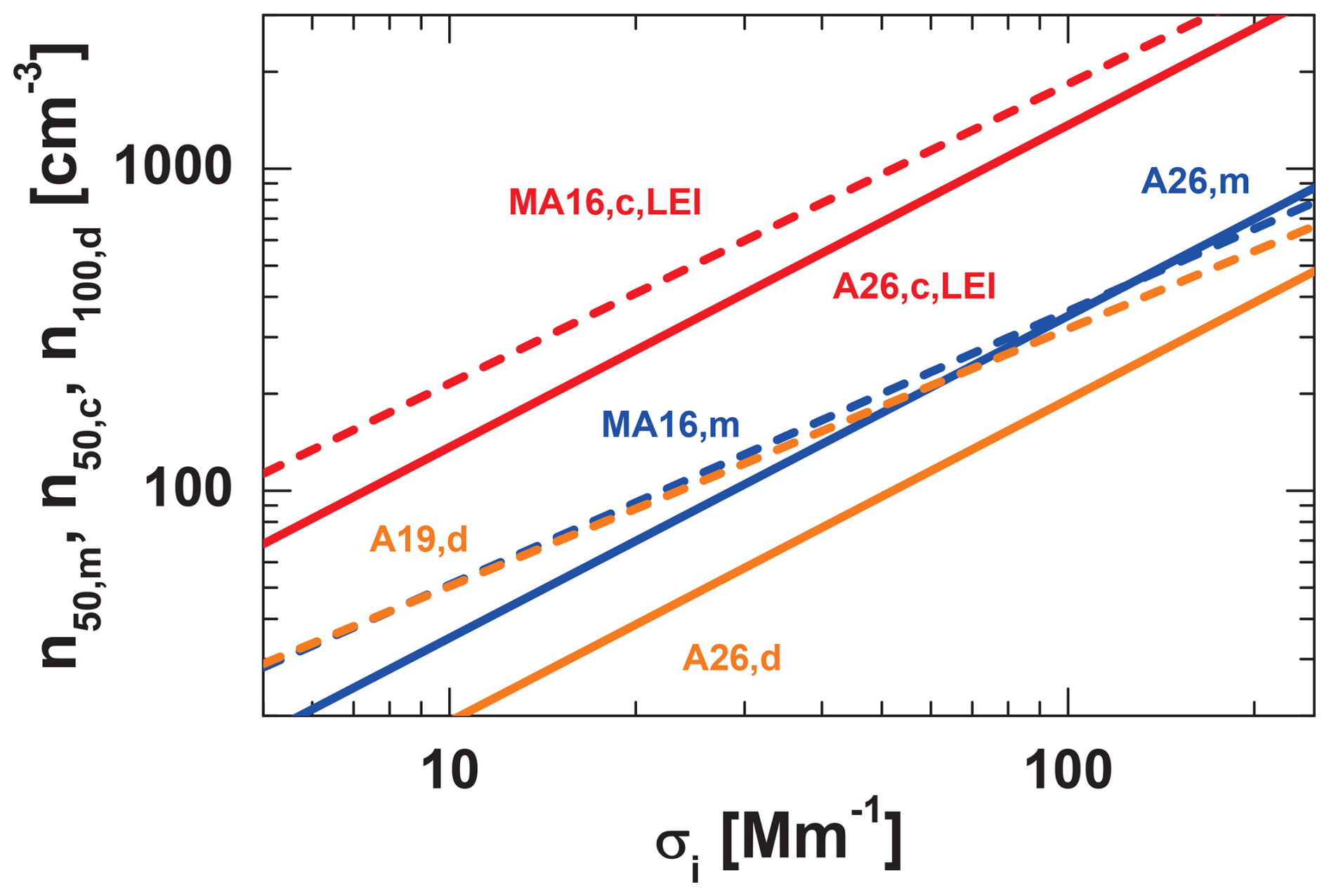
Figure 8 Particle number concentration (CCN proxy, dry particles) estimated from the 532 nm particle extinction coefficient by using the 2016 conversion method (MA16,m, marine, blue dashed; MA16,c,LEI, Leipzig urban haze, red dashed; A19,d, dust, orange dashed) (Mamouri and Ansmann, 2016; Ansmann et al., 2019b) and the new linear extinction-vs-number relationship (A26,m; A26,c,LEI; A26,d, solid lines), presented in this study (with the marine and dust conversion factors given in Table 13, and the Leipzig conversion factors in Table 11).

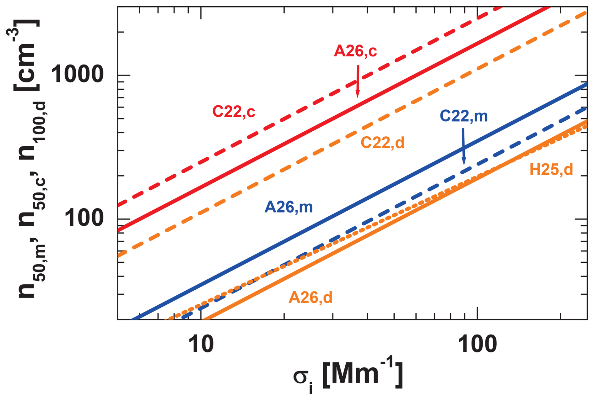
Figure 9 Comparison of the linear CCN-vs-extinction relationships applied by C22 (Choudhury et al., 2022) to estimate CCN concentrations from 532 nm extinction coefficients in the case of marine (C22,m, blue dashed), continental pollution (C22,c, red dashed), and dust particles (C22,d, orange dashed) and the respective relationships presented in this study (A26,m; A26,c; A26,d, solid lines, with the 532 nm conversion factors in Table 13). The dotted orange line shows the dust parameterization of He et al. (2025a), indicated by H25,d, derived from observations at a Saudi Arabian AERONET station.

In Fig. 8, we used c = 8.0 cm⁻³ and x_p=0.8 in the case of the A19,d line. The respective relationship between $n_{\mathrm{100},\mathrm{d},\text{dry}}$ and the 532 nm particle extinction coefficient σ_d,amb roughly represents the mean relationship between these two parameters when considering Saharan and Asian AERONET stations (Ansmann et al., 2019b).

The comparison of the different curves in Figs. 8 and 9 allows us to discuss the differences between the different conversion factors c_50,m, c_50,c, and c_100,d or, more general, the different conversion approaches when keeping the impact of the varying particle extinction exponent x_p into account.

The differences between the curves in Fig. 8 for a given aerosol type are to a large extent related to the changed statistical analysis applied to the AERONET observations. In our original approach (Mamouri and Ansmann, 2016; Ansmann et al., 2019b), we followed the recommendation of Shinozuka et al. (2015) and derived the respective extinction-to-CCN conversion factors from a linear correlation between, e.g., log(${\mathit{\sigma }}_{\mathrm{c},\text{amb},j}$) and log($n_{\mathrm{60},\mathrm{c},\text{amb},j}$) (see Table 6). Now, a weighted linear regression analysis is applied to the data fields of ${\mathit{\sigma }}_{i,\text{amb},j}$ and $n_{\mathrm{60},\mathrm{c},\text{amb},j}$, $n_{\mathrm{100},\mathrm{m},\text{amb},j}$, $n_{\mathrm{60},\mathrm{d},\text{amb},j}$, or $n_{\mathrm{100},\mathrm{d},\text{amb},j}$. This approach is much more simple and efficiently removes outliers. This change in the AERONET data analysis reduces the conversion factors by a factor of 1.4 to 1.8 (for extinction coefficients of 20–50 Mm⁻¹) in the case of continental pollution with Leipzig conversion factors (AE range from 1.6–2.0). The new approach significantly improved the POLIPHON conversion factors, which are now better in line with alternative conversion factors discussed by Kulkarni et al. (2025). In the case of mineral dust (A19,d vs A26,d), the conversion factors decreased by roughly a factor of 2 for dust extinction coefficients from 20–50 Mm⁻¹. Here, the problems with AERONET observations at high dust AOTs > 0.5, as discussed in Ansmann et al. (2019b), may have contributed to the strong deviation between the A19,d and A26,d curves. The MA16,m and A26,m curves for marine conditions are likewise close together. The remaining difference may indicate the impact of the different statistical analysis concepts, following Shinozuka et al. (2015) in the case of MA16,m and by applying the new linear regression approach in the case of A26,m.

In Fig. 9, we compare the updated POLIPHON approach to estimate CCN concentrations from lidar observations (A26,m; A26,c; A26,d) with an alternative approach (C22,m; C22,c; C22,d) introduced by Choudhury and Tesche (2022) and further discussed in Choudhury et al. (2022). In addition, we compare our updated CCN estimations (A26,d) with a parameterization for dust CCN (n_100,d) suggested by He et al. (2025a), indicated by He25,d and derived from AERONET observations in Saudi Arabia.

The C22 curves are based on conversion factors which are computed by using a specific particle size distribution for each aerosol type (dust, marine aerosol, polluted continental conditions). The microphysical properties for six different aerosol types of the CALIPSO aerosol model (CAMel) are used (Omar et al., 2005, 2009). CALIPSO stands Cloud-Aerosol Lidar and Infrared Pathfinder Satellite Observation (Winker et al., 2009, 2010). The differences between the curves for a given aerosol type i in Fig. 9 are mainly caused by the differences between the modeled CALIPSO size distribution and the climatological, real-world-reflecting size distributions for marine, dust, and continental haze aerosol derived from the AERONET long-term observations as used in our POLIPHON studies. The strong discrepancy between the dust conversion factors introduced by the underlying mineral dust size distribution characteristics was already discussed by He et al. (2025a). Obviously, the dust fine-mode fraction (particles with radius < 500 nm) of the CALIPSO aerosol model contains too many particles. The derived number concentration $n_{\mathrm{100},\mathrm{d},\text{dry}}$ is a factor of 6–7 larger than the respective A26,d values for extinction coefficients of 20–50 Mm⁻¹. Note, that our previous CCN estimation approach (Mamouri and Ansmann, 2016) already reproduced well airborne in-situ measured CCN concentrations as was shown in Choudhury et al. (2022).

A dust curve provided by He et al. (2025a), derived from AERONET observations in Saudi Arabia, is shown in Fig. 9 in addition. These authors used a different approach to filter out pure or almost pure dust observation. They used the depolarization information in the AERONET data base to filter out the observations dominated by dust. As can be seen, a very good agreement is found although the Shinozuka et al. (2015) approach is used, i.e., the retrieval of the extinction-to-n₁₀₀ conversion factor is based on the correlation between log(σ_d,j) and log($n_{\mathrm{100},\mathrm{d},j}$). This approach provides higher CCN concentrations at lower extinction coefficients.

Lenhardt et al. (2023) studied the relationship between in-situ-measured CCN concentrations in biomass burning smoke layers over the southeastern Atlantic west of southern Africa and 532 nm particle extinction coefficients measured simultaneously with lidar and found conversion factors c_50,bb close to 10 Mm cm⁻³. This is in reasonable agreement with our updated wildfire smoke conversion factors of 15.4 Mm cm⁻³ (for the mixture of fresh and aged tropospheric smoke), 10.9 Mm cm⁻³ (for fresh smoke in the UTLS) and 7.3 Mm cm⁻³ (aged smoke in the UTLS). The biomass burning smoke layers, observed west of Africa, may have even contained some dust particles contributing with rather low conversion factors of around 2 Mm cm⁻³ (Table 13) to the overall conversion factor.

Veselovskii et al. (2025) provided an independent multiwavelength-lidar-based approach to derive extinction-to-surface-area and extinction-to-volume conversion factors for aged wildfire smoke at 355 and 532 nm. These authors found c_s,bb of 1.3 Mm µm² cm⁻³ and c_v,bb of 0.085 Mm µm³ cm⁻³ for 355 nm and 1.75 Mm µm² cm⁻³ and 0.13 Mm µm³ cm⁻³ for 532 nm. Our updated 532 nm conversion factors are 1.98 Mm µm² cm⁻³ and 0.13 Mm µm³ cm⁻³, respectively.

Jäger and Deshler (2002, 2003) published conversion factors for the estimation of surface area concentrations in stratospheric sulfate layers after the strong volcanic eruption of the Pinatubo volcano in 1991. By combining balloon-borne observations of the stratospheric particle size distribution at Laramie, Wyoming, and lidar observations at Garmisch-Partenkirchen, Germany, a few months after the eruption Jäger and Deshler (2003) obtained for c_s,vs at 532 nm values of 2.5–3 Mm µm² cm⁻³. We obtained values of 1.55 Mm µm² cm⁻³ very shortly after the eruption of the Hunga Tonga volcano for very fresh sulfate layers, when the impact of sedimentation of sulfate particles only played a minor role. One year later, we derived a value of c_s,vs = 1.7 Mm µm² cm⁻³, when sedimentation and tropopause-fold events already removed the largest sulfate particles. For background conditions, the stratospheric sulfate conversion factors take values of 4–6 Mm µm² cm⁻³ (Jäger and Deshler, 2003).

5 Summary and concluding remarks

An updated set of POLIPHON conversion factors, applicable to lidar and ceilometer observations at the laser wavelengths of 355, 532, 911, and 1064 nm, has been presented. These conversion factors cover five aerosol types. In the case of volcanic ash (type number 6), the dust conversion factors can be used in conversion computations. A broad spectrum of robust, spectrally resolved, real-world-reflecting conversion factors is available for the use in the analysis of ceilometer and lidar network observations and spaceborne lidar data collected in the framework of several space lidar missions since 2006. To obtain the presented set of aerosol-type-dependent conversion factors measurements taken at 62 carefully selected AERONET stations, located in rather different environments around the globe, with data records typically covering 10–20 years, were statistically analyzed.

The main motivation for the update was given by the demands of the ceilometer and space lidar communities. By using the POLIPHON data analysis scheme, the ceilometer product spectrum can be significantly broadened towards CCN, INP, and mass concentration information. This potential may be used to support aerosol emission and transport modeling and weather predictions performed by environmental and meteorological services. Seifert et al. (2023) pointed out that actual aerosol conditions are not considered at all in numerical weather prediction models so that, e.g., strong Saharan dust outbreaks towards Europe, North America or Central and East Asia, which may have a strong impact on ice formation in the atmosphere, are completely ignored in weather forecasts. Meanwhile, powerful ceilometers are able to monitor desert dust outbreaks in large detail and, by using the POLIPHON method, even in terms of CCN and INP concentration estimates.

With respect to atmospheric research with focus on field studies of aerosol–cloud interaction, the updated POLIPHON conversion factors may contribute to a more robust and accurate characterization of the aerosol in terms of CCN and INP concentrations in the framework of closure studies, in which CCN and INP concentrations are compared with cloud droplet and ice crystals number concentrations obtainable from combinations of lidar and radar observations of cloud systems. Closure studies are of fundamental importance to better understand the impact of different aerosol and meteorological conditions on cloud and precipitation formation processes. Such closure studies are also possible from space, e.g., in the framework of the EarthCARE mission, so that a global view on aerosol–cloud interaction can in principle be reached with strong support by the POLIPHON methodology.

Appendix A: Conversion factors from LSE studies

The least-squares estimation (LSE) method (York et al., 2004) is applied to determine all conversion factors mentioned in Table 6. The respective input data sets x_i,j (particle extinction coefficient for aerosol type i and observations j from j=1 to j=N_obs) and y_i,j (one of the retrieved microphysical aerosol products for aerosol type i) are given in Table 6 (x_i,j and y_i,j columns).

For simplicity, we continue with x_j and x_j in this appendix, and leave out aerosol-type index i. The classical regression scenario is assumed (see Appendix D in York et al., 2004), i.e., we assume that the scatter of data points in the regression plots and in the obtained regression results are mainly caused by the uncertainty in the y_j data and not by the uncertainty in the observations x_j. We assume small uncertainties in x_j of 10 % or less. Such small uncertainties are confirmed by our numerous lidar-sunphotmeter intercomparisons we performed since more than 20 years. In contrast, large uncertainties of 20 % to 75 % are given for the AERONET products (Gerasopoulos et al., 2007; Dubovik and King, 2000; Dubovik et al., 2000, 2002, 2006).

The following set of equations are used to determine the conversion factors (York et al., 2004):

$$\begin{array}{}\text{(A1)}& {\displaystyle }& {\displaystyle }\stackrel{\mathrm{‾}}{y}=a+b\stackrel{\mathrm{‾}}{x},\text{(A2)}& {\displaystyle }& {\displaystyle }\stackrel{\mathrm{‾}}{x}={\displaystyle \frac{{\sum }_{j=\mathrm{1}}^N{w}_j{x}_j}{{\sum }_{j=\mathrm{1}}^N{w}_j}},\text{(A3)}& {\displaystyle }& {\displaystyle }\stackrel{\mathrm{‾}}{y}={\displaystyle \frac{{\sum }_{j=\mathrm{1}}^N{w}_j{y}_j}{{\sum }_{j=\mathrm{1}}^N{w}_j}},\text{(A4)}& {\displaystyle }& {\displaystyle }b={\displaystyle \frac{{\sum }_{j=\mathrm{1}}^N{w}_j\mathrm{\Delta }{x}_j\mathrm{\Delta }{y}_j}{{\sum }_{j=\mathrm{1}}^N{w}_j\mathrm{\Delta }{x}_j^{\mathrm{2}}}},\text{(A5)}& {\displaystyle }& {\displaystyle }a=\stackrel{\mathrm{‾}}{y}-b\stackrel{\mathrm{‾}}{x}\end{array}$$

with the intercept a, the regression coefficient b, the mean value $\stackrel{\mathrm{‾}}{x}$ of the independent variable, the mean value $\stackrel{\mathrm{‾}}{y}$ of the dependent variable, and $\mathrm{\Delta }{x}_j=x_j-\stackrel{\mathrm{‾}}{x}$ and $\mathrm{\Delta }{y}_j=y_j-\stackrel{\mathrm{‾}}{y}$. The determination of the weights w_j is explained below. The weights are used to widely suppress the impact of outliers in the y_j data set on the regression results, especially on the determination of the regression coefficient b.

The conversion factors are approximately given by the regression coefficient b, provided that the intercept a is close to zero. For a=0, $b=\stackrel{\mathrm{‾}}{y}/\stackrel{\mathrm{‾}}{x}$ according to Eq. (A1). The scatter in the y_j data causes a≠0.

The uncertainties of a and b are given by (York et al., 2004)

$$\begin{array}{}\text{(A6)}& \mathit{\delta }a=\sqrt{\sum _{j=\mathrm{1}}^N\mathrm{1}/\left(w_j\right)+{\stackrel{\mathrm{‾}}{x}}^{\mathrm{2}}\mathit{\delta }{b}^{\mathrm{2}}}\end{array}$$

and

$$\begin{array}{}\text{(A7)}& \mathit{\delta }b=\sqrt{\mathrm{1}/\sum _{j=\mathrm{1}}^N\left(w_j\mathrm{\Delta }{x}_j^{\mathrm{2}}\right)}.\end{array}$$

The coefficient of determination R² of the linear regression analysis is given by

$$\begin{array}{}\text{(A8)}& R^{\mathrm{2}}=\mathrm{1}-{\displaystyle \frac{{\sum }_{j=\mathrm{1}}^N{w}_j(y_j-\mathit{\beta }{x}_j{)}^{\mathrm{2}}}{{\sum }_{j=\mathrm{1}}^N{w}_j\mathrm{\Delta }{y}_j^{\mathrm{2}}}}\end{array}$$

with

$$\begin{array}{}\text{(A9)}& \mathit{\beta }={\displaystyle \frac{{\sum }_{j=\mathrm{1}}^N{w}_j{x}_j{y}_j}{{\sum }_{j=\mathrm{1}}^N{w}_j{x}_j^{\mathrm{2}}}}.\end{array}$$

The coefficient of determination R² expresses how well the dependent variable can be predicted by the observed, independent variable.

The required weights w_j in Eqs. (A2)–(A4) are obtained in the following way. We transferred all individual ratios $r_j=y_j/x_j$ to $r_j=y_{j,\text{ref}}/x_{\text{ref}}$, i.e., we relate all individual y_j values to the mean value $x_{\text{ref}}=\frac{\mathrm{1}}{N}{\sum }_{j=\mathrm{1}}^N{x}_j$. N is the number of available observations. The transferred values y_j,ref are given by

$$\begin{array}{}\text{(A10)}& y_{j,\text{ref}}={\displaystyle \frac{y_j}{x_j}}\times x_{\text{ref}}.\end{array}$$

Next, we defined the deviation

$$\begin{array}{}\text{(A11)}& \mathrm{\Delta }{y}_{j,\text{ref}}=y_{j,\text{ref}}-\stackrel{\mathrm{‾}}{y_{\text{ref}}}\end{array}$$

with the mean value $\stackrel{\mathrm{‾}}{y_{\text{ref}}}=\frac{\mathrm{1}}{N}{\sum }_{j=\mathrm{1}}^N{y}_{j,\text{ref}}$. The weight is then given by (York et al., 2004)

$$\begin{array}{}\text{(A12)}& w_j={\displaystyle \frac{\mathrm{1}}{(\mathrm{\Delta }{y}_{j,\text{ref}}{)}^{\mathrm{2}}}}.\end{array}$$

To avoid a too large impact of the data points y_j,ref close to the mean value $\stackrel{\mathrm{‾}}{y_{\text{ref}}}$ on the regression results because of the increasing weight with decreasing distance to $\stackrel{\mathrm{‾}}{y_{\text{ref}}}$, we set the weight to

$$\begin{array}{}\text{(A13)}& w_j={\displaystyle \frac{\mathrm{1}}{(y_{j,\text{ref}}*\mathrm{0.1}{)}^{\mathrm{2}}}}\end{array}$$

if the relative deviation $\mathrm{\Delta }{y}_{j,\text{ref}}/y_{j,\text{ref}}$ is between 0 and ± 0.1. Now, we can compute an improved mean value,

$$\begin{array}{}\text{(A14)}& \stackrel{\mathrm{‾}}{y_{\text{ref}}}={\displaystyle \frac{{\sum }_{j=\mathrm{1}}^N{w}_j{y}_{j,\text{ref}}}{{\sum }_{j=\mathrm{1}}^N{w}_j}}.\end{array}$$

In the following, we may apply Eqs. (A11)–(A14) many times before we proceeded with the regression analysis by using Eqs. (A1)–(A5).