Application of UAV-based methods for quantifying methane point source emissions over an Arctic geological seep

Uncrewed aerial vehicles (UAVs) are increasingly becoming essential monitoring tools across a rapidly growing set of applications, due to their operational versatility, relatively low operating cost, and provision of data at a range of spatial scales. However, UAV-based measurement methodologies and associated instruments for atmospheric research are still in their early stages and require extensive efforts to exploit their full potential. In Arctic regions, geological CH₄ seeps can release CH₄ at rates significantly higher than typical biogenic sources and those associated with permafrost degradation processes; hence, accurate quantification of their emission rates is crucial for the overall CH₄ budget of the Arctic. The application of conventional greenhouse gas monitoring platforms – flux chambers and eddy-covariance towers – are not always practical as eddy-covariance towers are stationary point measuring devices that require long observation times with reliable footprint modeling to constrain emissions while flux chambers have a small footprints and therefore require multiple measurements and have a high potential of introducing disturbances. UAVs can overcome these limitations as they can capture the spatial extent of the gas plume released from a point source with minimal disturbance to the source. In July 2025, we deployed two UAV platforms with different sensing instruments to sample a known geological CH₄ seep located at the outer Mackenzie River delta, Canada. We flew vertical “curtain” patterns with open-path and closed-path CH₄ instruments to sample gas concentrations in flux planes at different downwind distances from the gas seep. We first evaluated the performance of the UAV-mounted instrumentation, comparing the open- and closed-path greenhouse gas analyzers. We then applied two widely used quantification techniques (mass-balance and Gaussian plume inversion) finding that mass-balance approaches were better suited for flux estimation over the seep area as the measurements were not close to a Gaussian profile with an average model-data mismatch of 81 %. We estimate that the seep emission rate falls in the range of 7.8 to 16.0 kg CH₄ h⁻¹ and the average across all methods and flights were estimated as 12.3 kg CH₄ h⁻¹ with standard deviation of 2.4 kg CH₄ h⁻¹. The emissions from this single point are equivalent to the biogenic flux from approximately 2.5 km² of the surrounding permafrost landscape, underscoring the need to assess the potentially significant contribution of geological seeps to regional and pan-Arctic carbon budgets.

1 Introduction

Arctic permafrost ecosystems are subjected to warming about four times faster than the global average (i.e., Arctic amplification) (Rantanen et al., 2022), which results in accelerated permafrost degradation that may cause the decomposition of previously frozen carbon, amplifying the release of greenhouse gases (GHGs) such as CO₂ and CH₄. Additionally, permafrost and glaciers act as natural barriers that play a critical role in trapping large amounts of geological CH₄ below ground (Walter Anthony et al., 2012). As permafrost becomes unstable due to warming, this natural barrier is compromised. Fractures and conduits may develop or expand, facilitating the release of geological CH₄ into the atmosphere (Walter Anthony et al., 2012).

Geological CH₄ seeps are common in the outer Mackenzie River delta, and have been observed within channels, rivers, marshes, and lakes (Wesley et al., 2023; Dallimore et al., 2024). Due to limited accessibility and the risks of disturbing the source during the measurement, these surface waters constrains the methods that one can apply to quantify emissions, primarily due to limited accessibility and the risk of disturbing the source during the measurements. Thus far, locating and estimating the emission flux from these under water seeps has been challenging. Aerial imaging spectroscopy is poorly suited for this application due to water's extremely low reflectance in the shortwave infrared (Zhang et al., 2017; Baskaran et al., 2022; Ayasse et al., 2018; Elder et al., 2019). Airborne eddy covariance analysis lacks the spatial resolution that is required to resolve these point sources (Kohnert et al., 2017). Furthermore, conventional surface-based monitoring systems such as eddy covariance towers or flux chambers are impractical for locating and identifying new point or localized sources, and are generally more difficult to establish on bodies of water, wetlands, and marshlands. Accurately estimating the emission rates from point or localized sources if the locations are already known is less complex than unknown point sources, since this allows the monitoring systems to be positioned such that sources fall within their spatial coverage.

In contrast, small uncrewed aerial vehicles (UAVs) equipped with in-situ gas instruments are a very practical measurement alternative that can access hard-to-reach areas over bodies of water, wetlands, and marshlands. Small UAVs create minimal disturbance and can map the entire extent of a plume originating from a point source. Despite current limitations in their flight time, small UAVs are becoming an essential tool in atmospheric science (Thielicke et al., 2021; Wildmann and Wetz, 2022; Wetz et al., 2023, 2021; Bolek and Testik, 2022) and GHG emission measurements (Andersen et al., 2018, 2023; Gålfalk et al., 2021; Bolek et al., 2024; Bonne et al., 2024; Kunz et al., 2018, 2020; Shah et al., 2020; Scheller et al., 2022; Morales et al., 2022). Significant progress has been achieved in UAV-based emission quantification over industrial sites such as power plants and landfills (Shah et al., 2019; Gålfalk et al., 2021; Morales et al., 2022), however methodologies over natural ecosystems are still in the early stages of development (Bolek et al., 2024; Scheller et al., 2022; Shaw et al., 2021; Yazbeck et al., 2025).

Instrumentation for UAV-based GHG measurements must have high sensitivity, low power consumption, fast response time, and be lightweight. Gas analyzers based on absorption spectroscopy in the mid-infrared region using tunable diode lasers can meet these requirements and this is becoming a widely used technique to quantify the concentration of GHGs. For fast-moving aerial vehicles, such as UAVs, a critical choice must be made between open- and closed-path gas analyzers. While both rely on the same fundamental measurement principle, their gas sampling approaches differ, which influences data characteristics and processing requirements. The measuring cell of the open-path analyzers is directly exposed to the atmosphere, allowing near-instantaneous response to rapid changes in concentration caused by turbulence. Conversely, the enclosed sample cell in closed-path analyzers effectively smooths the measured concentration profiles due to the much lower air exchange rate in the sample cell and sampling tubes (Detto et al., 2011; Takriti et al., 2021). Closed-path analyzers typically feature temperature- and pressure-controlled sample cells, which minimize the impact of variable environmental conditions on measurement accuracy. However, the necessary sampling pumps and thermal regulation systems increase instrument weight and power consumption compared to open-path alternatives. Conversely, open-path analyzers are directly exposed to changing atmospheric conditions that can affect their performance, often requiring post-acquisition corrections.

Beyond monitoring system considerations, the choice of data analysis method is critical for accurately quantifying fluxes. One well-established technique to quantify emission rates from mobile platforms is the mass balance approach (Morales et al., 2022; Andersen et al., 2023; Bonne et al., 2024). In this method, the emission rate is estimated by integrating the enhanced concentration signal over the observational plane (Bonne et al., 2024). This method usually requires interpolation of the non-uniform sparse UAV measurements onto a uniform 2D-grid using techniques such as the Kriging method (Morales et al., 2022; Andersen et al., 2021). Fitting a covariance model to a geo-spatial dataset requires the user to optimize predefined variances and length scales, as the covariance model is highly sensitive to these parameters (Morales et al., 2022). The mass balance technique can also be applied without using a complicated interpolation scheme, provided that the collected data have high spatial resolution (Bonne et al., 2024; Scheutz et al., 2025; Borchardt et al., 2025). In this direct approach, horizontal flight transects are treated individually, and transect-integrated flux densities are interpolated between each transect, and extrapolated between the lowest-altitude transect and the ground. Gaussian plume inversion is another widely used approach to quantify the emission rates using UAVs (Shah et al., 2019; Andersen et al., 2021). In this technique, the concentration profile generated by emissions from a constant point source is assumed to be time-invariant and to follow a Gaussian distribution. UAV-based sampling close to the source may not always yield a Gaussian-like concentration field due to small-scale turbulence, short observation times, and insufficient repeated measurements; however, several studies have shown that this method can be used to generate reasonable flux estimates (Shah et al., 2019, 2020; Andersen et al., 2021). Both the Gaussian plume inversion and mass balance approaches require wind speed data in addition to concentration measurements.

In this study, we deployed two UAV platforms, one equipped with an open-path instrument and the other with a closed-path instrument, to quantify the source strength of a geological CH₄ seep. We applied three emission rate quantification methods to the measured data: mass balance with Kriging interpolation, direct mass balance, and Gaussian plume inversion. Finally, we discussed the results obtained from the two gas analyzers and the different quantification methods, evaluating their advantages and disadvantages for UAV-based applications over the seep site, which are relevant to applications in other sectors where CH₄ emissions are a concern.

2 Methods

2.1 Measurement site, UAV platforms, and sampling strategies

Our study site is a known geological CH₄ seep located at the outer Mackenzie River delta, west of Richards Island, Northwest Territories, Canada (69.319583° N, 135.477520° W), where there is an abundance of water bodies throughout the extensive wetlands (Fig. 1a). Permafrost underlying the Arctic's second largest delta is relatively thin (<100 m) and formed during the Holocene (Burn and Kokelj, 2009; Dallimore et al., 2024). While several parameters influence the permafrost thermal state, including snow cover, vegetation, and ground temperature, hydrology exerts the greatest influence on the local ground thermal regime (Burn et al., 2009; Burn and Kokelj, 2009; Miner et al., 2022). We focus on a seep previously identified and named Channel Seep 2 (Wesley et al., 2023; Dallimore et al., 2024), which originates from the riverbed. The maximum measured gas seepage rate was reported as 0.4 m³ min⁻¹, which is equivalent to 16.1 kg h⁻¹, assuming all the seepage consists of CH₄ with a density of 0.67 kg m⁻³ (see Fig. 1b) (Dallimore et al., 2024). Across the outer Mackenzie River Delta, Dallimore et al. (2024) documented 46 natural gas seeps with diverse characteristics in geological formation via isotopic signatures, occurrence, and size. Strong CH₄ emissions throughout this thin permafrost area were previously detected by the Polar 5 research aircraft (Kohnert et al., 2017) and attributed to geological sources based on emission rates much higher than typical biogenic sources. This attribution was later confirmed by isotopic analysis (Dallimore et al., 2024; Wesley et al., 2023). Although there are several other seeps in this region, to the best of the authors' knowledge, there is no close strong source in the downwind direction that can significantly influence the measurements of this study. We rarely observed sporadic ebullition events from a pond close to Channel Seep 2; however, these ebullition events compared to main seep were minuscule and expected to have a negligible impact on the flux estimations.

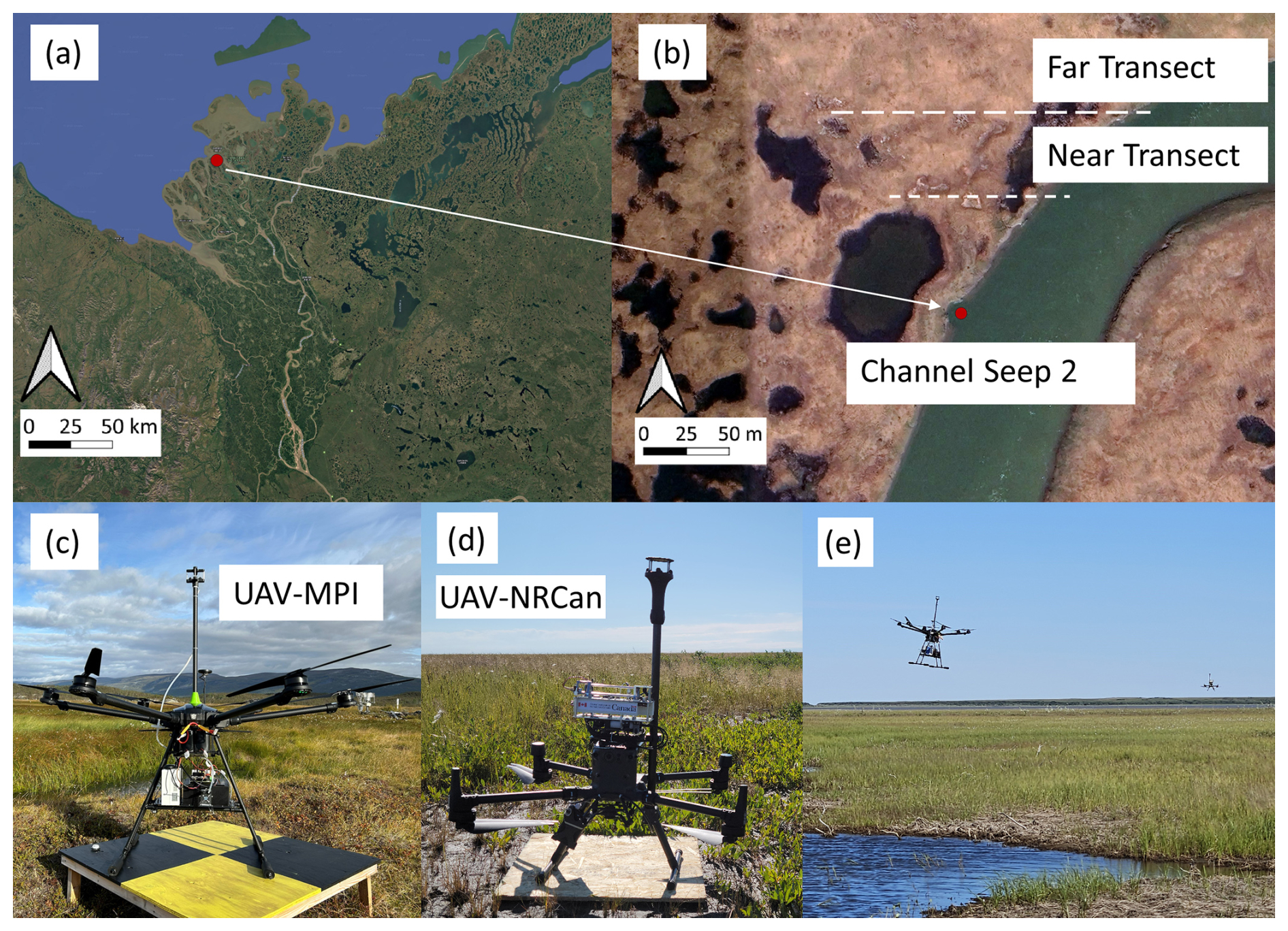
Figure 1 Study area in the outer Mackenzie River delta, NT, Canada (a); Aerial image of the location of Channel Seep 2 (69.319583° N, 135.477520° W) indicated by red dot and approximate transects flown indicated by dashed lines (b) ((a) and (b) overlaid on satellite images, Maps data: ©Google Maps 2025, Imagery: ©2025 Airbus, Maxar Technologies); Images showing the two UAV platforms, UAV-MPI (c, figure adapted from Bolek et al. (2024)) and UAV-NRCan (d). Image (e) shows the two UAVs sampling downwind of CH₄ seep in the near (UAV-MPI) and far (UAV-NRCan) distances.

To quantify the emission rate at Channel Seep 2, we used two UAV platforms: UAV-MPI (Fig. 1c) and UAV-NRCan (Fig. 1d). UAV-MPI is a hexacopter (PM X6 Pro XL) that is equipped with CH₄ and CO₂ gas analyzers along with an ultrasonic anemometer (Licor LI-550) that measures 2D wind speed, temperature, humidity, and pressure (see Bolek et al., 2024 for more details). The CH₄ analyzer is a closed path (CP) analyzer (Strato, Aeris Technologies) that measures the dry mole fraction of CH₄ at 2 Hz sampling frequency with <1 ppb s⁻¹ of sensitivity. The CP instrument was customized by adding a thermally controlled enclosure to control the temperature of the measuring cell, which reduces the instrument drift (see Appendix A). The anemometer deployed on UAV-MPI, 0.67 m above the rotor plane, recorded wind measurements at 2 Hz with a reported accuracy of ±0.2 m s⁻¹ for speed and ±1.0° for direction. UAV-NRCan is a DJI Matrice 300 RTK quadcopter equipped with a CH₄ gas analyzer custom-built by the National Research Council of Canada (NRC), and a 2D anemometer (WindUltra, Gill Instruments) placed 0.75 m above the rotor plane to measure wind speed and direction. The NRC CH₄ analyzer is a mid-infrared tunable diode laser absorption spectroscopic system with an open path (OP) gas cell, a sampling rate of 100 Hz, and a resolution of 26 ppb at 10 Hz, calibrated over the concentration range of 2 to 50 ppm (Beattie et al., 2026), and the anemometer has an accuracy of <2 % RMSE for wind speed and <1.0° RMSE for wind direction. Two additional ground-based wind sensors were deployed to verify the UAV-based measurements. The wind speed measurements are relatively consistent between the UAV platforms, and the wind conditions are similar for the far- and near-curtain flights. More details can be found in Appendix D, where the measurements of ground-based sensors were also included. With the full scientific payload, each UAV platform achieved flight times of about 20 min.

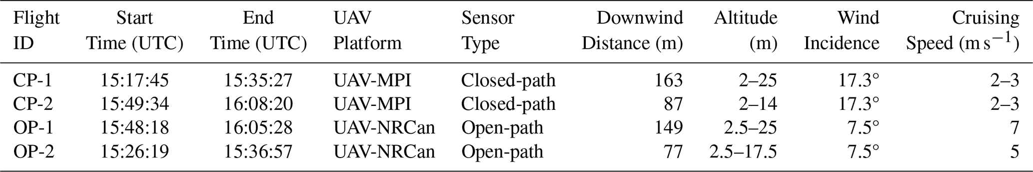
We conducted a total of four flights, with each UAV platform flying curtains at two distances from the Channel Seep 2, corresponding to roughly 80 and 150 m downwind (Fig. 1b). Table 1 shows the flight details. Flight curtains were oriented to be approximately perpendicular to the local wind direction. The lowest flight transects were conducted as close to the ground surface as possible to minimize quantification uncertainty associated with a near-ground measurement gap. UAV-MPI (flight IDs CP-1 and -2) was flown manually, since programming flight pattern on-site was not possible for this UAV, at a constant speed while maintaining a fixed heading. UAV-NRCan (flight IDs OP-1 and -2) was flown with a pre-programmed flight trajectory where the headings aligned with the direction of UAV travel. The width of the far curtains for both platforms (CP-1 and OP-1) was approximately 250 m. The near curtain width (CP-2 and OP-2) was approximately 150 m.

Table 1 Details of the conducted flights, all flights were performed on 1 August 2025. Mean air temperature during flights was about 19 °C.

All four curtain flight transects are shown in a top-down “bird's-eye” view in Fig. 2. The x-axis is defined to align with the mean prevailing wind direction for all flights, which is 188.5°. The downwind distance from the source (i.e., seep location) to each flux curtain along the x-axis is indicated. Along the central axis, the curtains flown by closed-path UAV-MPI (CP-1 and CP-2) are 10–14 m farther from the source than the corresponding curtains for open-path UAV-NRCan (OP-1 and OP-2), but in all cases the flight transects extended beyond the boundaries of the plume. In all curtains, the dominant wind direction approximately coincides with the location of the observed CH₄ peak enhancements along the transects. The mean wind incidence angle was <20° in all cases (see Fig. 2 and Table 1) and the non-zero wind incidence angle is expected to have a negligible impact on the emission rate calculation (Mohammadloo et al., 2025). For all our quantification methods, we assumed that the seep source as well as the channel flow rate is time-invariant during the sampling period.

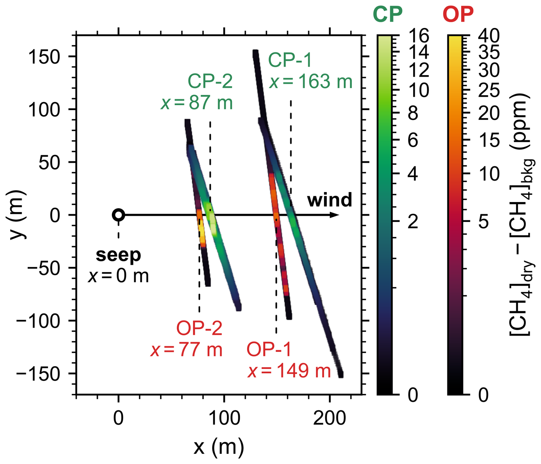
Figure 2 Bird's-eye view of measured methane concentrations after removing the background for the four curtain flights. The origin of the coordinate system is defined at the gas seep (69.319583, −135.477520°) and the x-axis is aligned with the dominant wind direction (188.5°). Here, OP and CP indicate open-path and closed-path and refer to UAV-NRCan and UAV-MPI, respectively.

2.2 Flux quantification methods

2.2.1 Mass balance approach

The mass balance approach is widely used to estimate net emissions released from a point source or a defined area, and the mass conservation equation is typically simplified by neglecting diffusion and assuming the plume is statistically stationary during the sampling period. We applied a mass balance approach to UAV-based sampling similar to the approach used in piloted aircraft-based sampling (Karion et al., 2013; Fiehn et al., 2020). The mass balance method applied to piloted aircraft-based sampling often requires, or assumes, a vertically well-mixed boundary layer since measuring a plume's vertical variability is not always possible (Karion et al., 2013; Fiehn et al., 2020). Although at sufficiently downwind distances this assumption may hold, for UAVs where the sampling being made close to the source, the plume is most likely not vertically well-mixed, hence dense sampling along vertical and horizontal axes are required (Shaw et al., 2021). The net emission flux (Q) through a sampling plane transecting the plume is given by:

$$\begin{array}{}\text{(1)}& {\displaystyle }Q=\int \int q_{\mathrm{meas}}(y^{\prime },z)\mathrm{d}{y}^{\prime }\mathrm{d}z\end{array}$$

where the flux plane is defined along the measured transect (y^′) and altitude (z), and $q_{\mathrm{meas}}(y^{\prime },z)$ is the CH₄ flux density at each point in the flux plane, as defined in Eq. (2) below. Note that y^′ is curtain-specific, as it is derived from the UAV's flight path. The flux densities are given by:

$$\begin{array}{}\text{(2)}& \begin{array}{rl}{q}_{\mathrm{meas}}(y^{\prime },z)& =\left(\right[{\mathrm{CH}}_{\mathrm{4}}{]}_{\mathrm{meas}}(y^{\prime },z)-\left[{\mathrm{CH}}_{\mathrm{4}}{]}_{\mathrm{bkg}}\right)\\ & \cdot u_{⟂}(y^{\prime },z)\cdot {\mathit{\rho }}_{{\mathrm{CH}}_{\mathrm{4}}}\left(z\right),\end{array}\end{array}$$

where [CH₄]_meas is the measured CH₄ mixing ratio, [CH₄]_bkg is the background mixing ratio. A constant background CH₄ of 2031.8 and 2029.1 ppb is removed from the measured dry mole fractions for UAV-MPI and UAV-NRCan, respectively, where these background values were estimated by averaging sampling points outside of the plume-affected regions (see also Fig. B1). u_⟂ is the component of the recorded wind speed perpendicular to the flux curtain, and ${\mathit{\rho }}_{{\mathrm{CH}}_{\mathrm{4}}}\left(z\right)$ is the density of CH₄ gas, used to convert the CH₄ mixing ratio [ppm] to mass concentration [gCH₄ m⁻³], which is calculated according to:

$$\begin{array}{}\text{(3)}& {\mathit{\rho }}_{{\mathrm{CH}}_{\mathrm{4}}}\left(z\right)={\displaystyle \frac{P\left(z\right)M_{{\mathrm{CH}}_{\mathrm{4}}}}{R{T}_{\mathrm{avg}}}}(\mathrm{100}\mathit{\%}-{\mathrm{H}}_{\mathrm{2}}\mathrm{O}(y,z\left)\right)\end{array}$$

where P(z) is the altitude-dependent pressure, H₂O(y,z) is the measured water vapor mole fraction in percentage, $M_{{\mathrm{CH}}_{\mathrm{4}}}$ is the molar mass of CH₄ (16.04 g mol⁻¹), R is the universal gas constant (8.314 m³ Pa K⁻¹ mol⁻¹), and T_avg is the average temperature. P(z) is a regression function that was derived from pressure measurements of UAV-NRCan, and T_avg was calculated using the ground sensor measurement.

In this study, we used two different mass balance approaches to estimate the emission rate: direct mass balance (DMB), Sect. 3.2.1, and cluster Kriging mass balance (CKMB), Sect. 3.2.2. The DMB approach uses the measured enhancements without any in-plane interpolations. In DMB, transect integrated flux densities ($\int q_{\mathrm{meas}}\mathrm{d}{y}^{\prime }$ in gCH₄ s⁻¹ m⁻¹) are calculated using simple linear interpolation, for each horizontal transect and then subsequent integration carried out in the vertical direction. At the lowest level of the sampling plane, we used a logarithmic function to complete the vertical profile, assuming zero flux at the ground level (Bonne et al., 2024; Dooley et al., 2024). Given that the methane source is effectively at ground level, high CH₄ mixing ratios are expected close to the ground, and so the shape of the extrapolation curve is convex. The CKMB approach, on the other hand, uses Kriging interpolation to map the measured CH₄ enhancement onto a regular grid. Kriging is a technique that employs an interpolation based on predefined covariance models (Müller et al., 2022). We used the cluster Kriging method that was developed by Morales et al. (2022) and first clustered the data into two groups, enhanced and background, using a Gaussian Mixture Model. We fit the data within each cluster with a variogram (scikit-gstat analysis module was used), optimizing the variance and length-scales through least-square regression. We exported the fitted variograms to covariance models (gstools library), which we later used to apply Ordinary Kriging (pykrige library). We interpolated the measured wind field onto the same grid as the concentrations; however in this case, we applied ordinary Kriging without clustering the data as clustering is not required for wind data. In both mass balance methods, the surface is treated as homogeneous and flat.

The uncertainties are attributed to instrument errors, interpolation errors, plume capture uncertainty, background concentration estimation, and non-stationary plume dynamics. The instrument errors of OP and CP analyzers were detailed in Beattie et al. (2026) and in Bolek et al. (2024), as well as in Appendix A, respectively. In the CKMB method, the uncertainties are quantified using the covariance matrices provided by the Kriging algorithms, which were below 10 % of the calculated emission rates for all cases. For the DMB method, the uncertainties associated with linear interpolation along the vertical and horizontal axes are assumed to be around 10 % as was found in the Kriging algorithm uncertainties. Due to the high-resolution sampling and because the choice of interpolation techniques has been shown to have a negligible impact on the emission rate estimation (Mohammadloo et al., 2025), we assigned similar-magnitude interpolation uncertainties for both mass balance methods. Since the interpolation uncertainties were readily available from the CKMB method, we applied the same range for the DMB method. This assumption could be significantly violated in the case of low-resolution UAV sampling. In this case, a more rigorous uncertainty quantification approach would be required. Plume capture uncertainty arises when the UAV misses the plume on one or more transects. Here, we quantify this uncertainty by leaving one transect out and running the algorithm again. The estimated flux values are about 20 % smaller when the transect with the highest CH₄ enhancement is excluded. Overall, we conservatively estimate the uncertainty contribution from the plume capture component to be 25 % of the calculated flux values. Using constant background concentration may cause bias in our flux estimations as background concentration may vary. To account for this in our uncertainty budget, we used ±1σ of the background concentration and propagated this as a systematic error source in our flux estimations (Yong et al., 2024). This yielded about 3 % additional uncertainty for CP flux estimates and between 10 %–13 % for OP flux estimates as ±1σ corresponds to about 3 ppb for CP and 9 ppb for OP analyzer. We note that this difference between the sensors originates from different noise characteristics of the sensors rather than being a physical difference in background. The uncertainties originating from the turbulent nature of the atmospheric transport however, are challenging to quantify and were not included in the uncertainty estimation here.

2.2.2 Gaussian plume inversion approach

The Gaussian plume model provides a simplified solution for the advection-diffusion equation and is used to simulate the atmospheric transport of GHGs such as CH₄. In the Gaussian plume model, the concentration field is assumed to be steady-state, meaning that the wind field is stable over time, such that the concentration field is time invariant and the surface is treated as homogeneous and flat. However, this assumption may not hold under turbulent and variable wind conditions, especially close to the source (Shah et al., 2019). Several formulations have been proposed to overcome this issue, such as replacing the diffusivity parameter with a near-field mixing factor (Shah et al., 2019) or applying a different dispersion calculation than the Gaussian plume formulation (Vergassola et al., 2007; van Hove et al., 2025). Here, we adapt the approach from Shah et al. (2019) where the time-averaged flux density is presumed to follow from the morphology of a Gaussian plume, such that the modeled flux density (q_mod) is given by:

$$\begin{array}{}\text{(4)}& \begin{array}{rl}{q}_{\mathrm{mod}}(x,y,z)& ={\displaystyle \frac{Q}{\mathrm{2}\mathit{\pi }{\mathit{\sigma }}_y\left(x\right){\mathit{\sigma }}_z\left(x\right)}}\exp \left(-{\displaystyle \frac{(y-y_{\mathrm{0}}{)}^{\mathrm{2}}}{\mathrm{2}{\mathit{\sigma }}_y^{\mathrm{2}}\left(x\right)}}\right)\\ & \left\{\exp \left(-{\displaystyle \frac{(z-h{)}^{\mathrm{2}}}{\mathrm{2}{\mathit{\sigma }}_z^{\mathrm{2}}\left(x\right)}}\right)+\exp \left(-{\displaystyle \frac{(z+h{)}^{\mathrm{2}}}{\mathrm{2}{\mathit{\sigma }}_z^{\mathrm{2}}\left(x\right)}}\right)\right\}\end{array}\end{array}$$

where Q is the total emission flux from the CH₄ source, σ_y(x) and σ_z(x) are the horizontal and vertical mixing factors, y₀ is the center of the plume along the y-axis, and h is the height of the emission source. We assume that the mixing factors σ_y(x) and σ_z(x) vary linearly with distance x from the source, such that σ_y(x)=τ_yx and σ_z(x)=τ_zx.

Given experimentally determined flux densities over a measured flux curtain, the emission rate through the flux curtain can be estimated by fitting Eq. (4) to the measured data. The flux densities can be computed from measured concentration data [CH₄]_meas according to:

$$\begin{array}{}\text{(5)}& \begin{array}{rl}{q}_{\mathrm{meas}}(x,y,z)& =\left(\right[{\mathrm{CH}}_{\mathrm{4}}{]}_{\mathrm{meas}}(x,y,z)-\left[{\mathrm{CH}}_{\mathrm{4}}{]}_{\mathrm{bkg}}\right)\\ & \cdot u_x(x,y,z)\cdot {\mathit{\rho }}_{{\mathrm{CH}}_{\mathrm{4}}}\left(z\right)\end{array}\end{array}$$

This definition is similar to that for flux density given in Eq. (2), except that we replace the perpendicular wind speed with u_x, which is the x-component of instantaneous wind vector, where x is aligned with the prevailing wind direction (see Fig. 2). In this work, the CH₄ source is a gas seep in a water channel, and so we fix h=0. We fit the remaining parameters Q, y₀, τ_y, and τ_z using the LMFIT package in Python. The uncertainty in the emission rate can be estimated by evaluating how well the model fits the measured data (Shah et al., 2019) such that:

$$\begin{array}{}\text{(6)}& \mathrm{\Delta }Q=Q\sqrt{{\displaystyle \frac{{\sum }_j\left((q_{\mathrm{meas},j}-q_{\mathrm{mod},j}{)}^{\mathrm{2}}\right)}{{\sum }_j\left(q_{\mathrm{meas},j}^{\mathrm{2}}\right)}}}\end{array}$$

This formulation for the uncertainty in Q accounts for both the variability in wind direction and the uncertainty in the positional data. We assume that uncertainties in the measurements of CH₄ concentration, wind speed, temperature, and pressure are negligible compared to the uncertainty in the model itself, and that the frequency of spatial sampling is sufficient to avoid any bias in flux estimation.

3 Results and Discussions

3.1 Comparing sensor response and wind measurements between UAV platforms

Both UAV-platforms were instrumented with an anemometer and CH₄ analyzer. The measured wind speed and direction for each system are corrected to account for the velocity of the UAV platform. Measured wind speeds from all four curtain flights are illustrated as a function of altitude in Fig. 3 (see also Appendix D). The wind speed measurements are relatively consistent between the UAV platforms, and the wind conditions are similar for the far- and near-curtain flights. Both platforms show large wind speed variability at each altitude, with average standard deviations of 0.68 and 0.64 m s⁻¹ for UAV-MPI (CP-1 and CP-2) and UAV-NRCan (OP-1 and OP-2) at both curtains, respectively. Following Bolek et al. (2024), assuming a neutral boundary layer condition and logarithmic wind profile, we estimate the friction velocity u^* from the measured wind speed profile for each curtain (see Fig. 3). These values (u^*) are very similar across all flights, indicating comparable turbulence conditions. The uncertainty in u^* is smaller for UAV-NRCan compared to UAV-MPI, which can primarily be attributed to denser measurements in the vertical direction and faster movement of the UAV-NRCan. We correct UAV-MPI wind direction measurements for misalignment of the wind sensor relative to north, to yield mean wind directions of 189.8° ± 10.8°, 189.1° ± 11.9°, 188.0° ± 7.9°, and 189.0° ± 7.9° for CP-1, CP-2, OP-1, and OP-2, respectively.

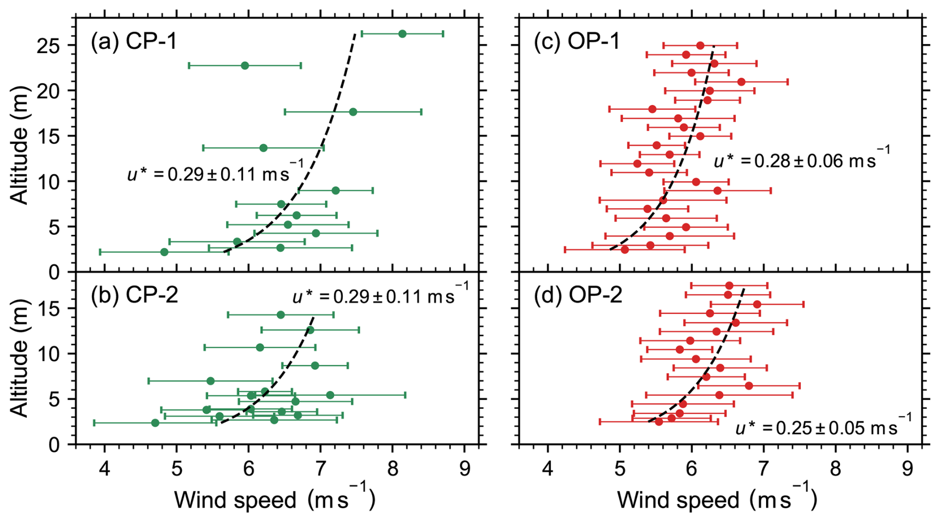
Figure 3 Measured wind speed and estimated friction velocities from (a, b) UAV-MPI and (c, d) UAV-NRCan. Closed circles represent mean wind speed at each altitude while standard deviations are represented as horizontal bars. The black dashed lines represent the logarithmic fitting. The flight ID is indicated in the top left corner for each flight (see Table 1).

Figure 4 shows the CH₄ enhancements measured in each of the four curtain flights as a function of position in the curtain. The corresponding timeseries data is shown in the Appendix (Fig. B1). As UAV-MPI (CP-1 and CP-2) was piloted manually, the horizontal transect length and vertical spacing are less regular than for UAV-NRCan (OP-1 and OP-2), which used pre-programmed flights. In both cases, i.e. manual and pre-programmed flights, we ensured that the extents of the plume were captured by monitoring the sensors' data over a radio link in real-time. In addition, after the initial CP-2 curtain flight was complete (at around 15 m above takeoff), UAV-MPI repeated the lower transects at the bottom of the curtain and collected additional data until its battery was depleted. The measured peak CH₄ enhancements for both OP curtains are 2–3 times larger than those measured in the CP curtains. Morales et al. (2022) observed similar differences between an active AirCore system and a custom-built, open-path quantum cascade laser absorption spectrometer (QCLAS). These differences in the measured mixing ratios can mainly be attributed to instrument characteristics of the CP analyzer, including cell volume and flow rate. Although the measured peak mixing ratios are affected by the instrument characteristics, the integrated area should not be affected (Tettenborn et al., 2025). In our analyses, we verify this by comparing the emission rate estimations between these sensors. The peak concentration enhancements measured in the far curtain flights CP-1 and OP-1 are 8.1 and 17.3 ppm, respectively. For the near-curtain flights, the peak enhancements are 19.7 and 47.8 ppm for CP-2 and OP-2, respectively. The altitudes corresponding to the transects containing the peak concentrations are similar for both platforms: 5.2 and 6.0 m for the far curtains CP-1 and OP-1, and 3.2 and 3.4 m for the near curtains CP-2 and OP-2, respectively. Rather than indicating a substantial difference in the actual CH₄ concentration, the higher concentrations measured by the OP sensor are indicative of its much faster response time and lack of an enclosed sampling cell compared to the CP sensor. The limited pump speed and mixing within the enclosed sampling cell for the CP sensor result in an effective smoothing and broadening of the measured data. For this reason, distinct color scales are defined for the CP sensor curtains and the OP sensor curtains, capped at 16 and 40 ppm for CP and OP, respectively.

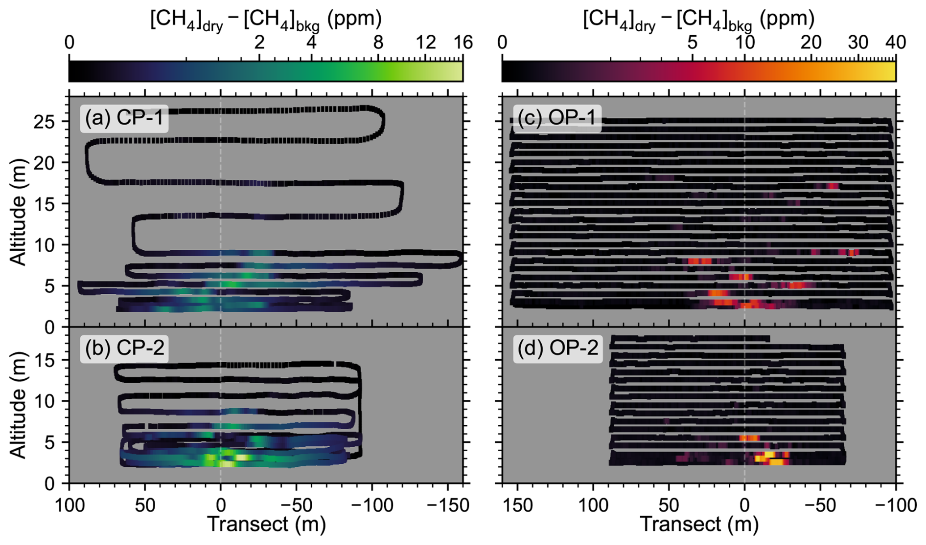
Figure 4 Measured dry methane concentrations after removing the background for the four curtain flights. (a, b) Curtains for the closed-path sensor at downwind distances of 163 and 87 m, respectively. (c, d) Curtains for the open-path sensor at 149 and 77 m downwind.

To compare the performance of the closed path (CP; UAV-MPI) and open path (OP; UAV-NRCan) analyzers, we examine the transects around the same altitude (around 3 and 5 m a.g.l.). The comparison is shown in Fig. 5a and b for far and near curtains, respectively. To facilitate comparison, the measured CH₄ concentration is plotted as a function of distance Δy relative to the peak along the y-axis (as defined in Fig. 2). The direction of travel along the transect for each UAV is indicated by an arrow in the legends of Fig. 5a and b. In general, the signal from the OP analyzer shows much higher temporal resolution and associated fluctuations compared to CP, for which the measurements were much smoother. The width of the signal of both analyzers is more similar for the far curtain (OP-1 and CP-1) than for the near curtain. This is because the plume is more evenly dispersed at further distances from the source. Both sensors observe additional peaks on both sides of the central peak that are attributed to the plume meandering under turbulent conditions. However, the shape of the plume recorded by the CP sensor is consistently asymmetrical with a gradual tail appearing after the UAV has crossed the plume (see Figs. 5 and B1). This asymmetrical tailing towards the flight direction is attributed to air mixing in the analyzer cell and, to a large extent, due to the slow air exchange rate of the CP analyzer (i.e. 0.7 Hz at 0.6 L min⁻¹ of flow rate). We do not expect that this tailing would cause significant bias in our emission rate estimations, as integrating along a transect should yield similar results, irrespective of the instrument response time (Tettenborn et al., 2025). Apart from the smoothing and broadening of the measured data, the extended tail of the CP measurement has additional smaller secondary peaks along the flight direction which may be attributed to (i) a slightly larger wind-incidence angle–supported by the shorter tail in the opposite flight direction, (ii) limited pump speed and/or friction within the tubing that prevents complete flush of the sampled air effectively.

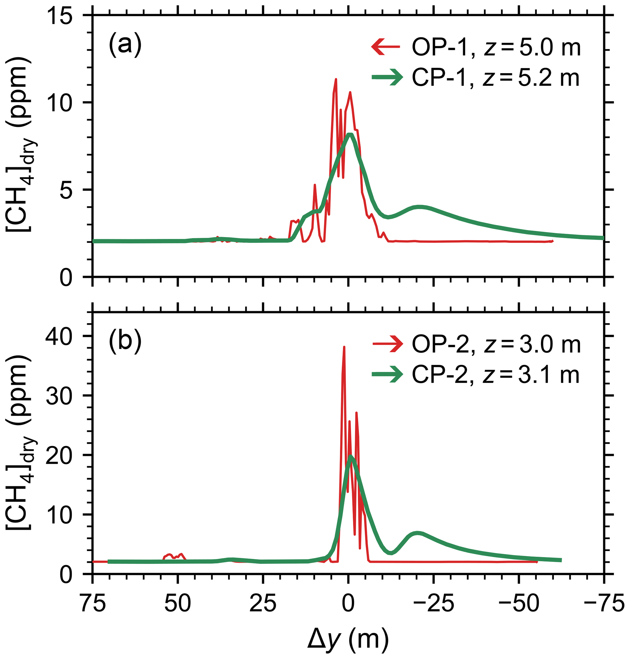
Figure 5 Comparison of dry methane concentrations measured by the closed- and open-path sensors over a single horizontal transect. (a) Horizontal transects measured at z≈5 m above ground-level for downwind distances of 163 m (CP-1) and 149 m (OP-1). (b) Transects at z≈3 m for 87 m (CP-2) and 77 m (OP-2). To facilitate comparison, the horizontal axis shows the distance Δy relative to the recorded peak. Arrows in the legends indicate the flight directions.

3.2 Emission flux quantification

3.2.1 Direct mass balance

The calculated transect integrated flux densities (i.e., $\int q_{\mathrm{meas}}\mathrm{d}{y}^{\prime }$) for all curtains are illustrated in Fig. 6. In all flights, the flux profiles converge to zero with increasing altitude, indicating that the plume extent in the vertical direction is fully captured. Using the DMB method, the emission rate of the seep is calculated to be 11.7±5.5 kg CH₄ h⁻¹ and 13.5±7.9 kg CH₄ h⁻¹ from CP-1 and CP-2, respectively. For OP-1 and OP-2, the calculated emission rates are 10.0±6.2 kg CH₄ h⁻¹ and 12.1±8.8 kg CH₄ h⁻¹, respectively. For the far curtains (CP-1 and OP-1), minor enhancements are detected even above 15 m a.g.l., whereas for the near curtains (CP-2 and OP-2), no enhancement is captured above 10 m. Due to atmospheric turbulence, at some altitudes both platforms miss the plume, with only minimal enhancements observed at 5.5 m for CP-2, at 7 m for OP-1, and at 4.5 m for OP-2. As UAVs capture only the instantaneous plume, these events are unavoidable. However, dense vertical sampling and repeated measurements can minimize the impact of missing the plume; still, we estimate that missed plume sections contribute at most about 25 % uncertainty (see Sect. 2.2.1) to the emission flux values reported here.

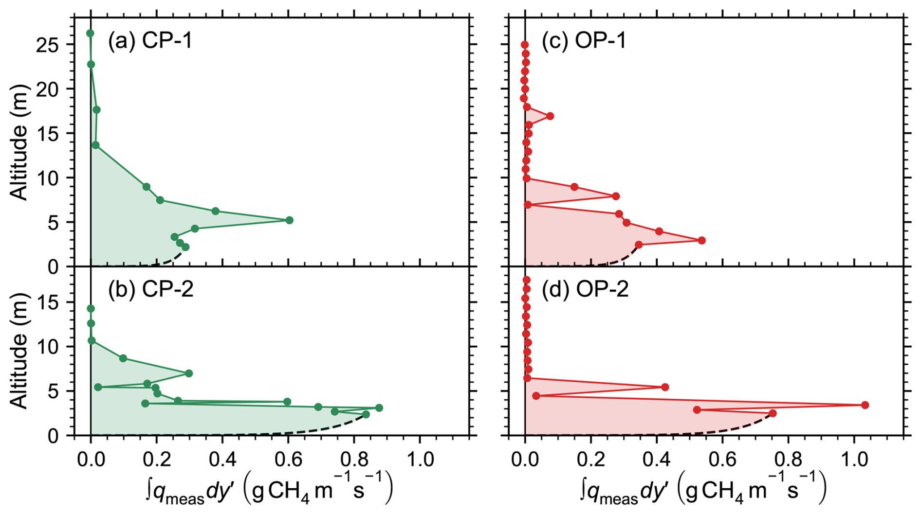
Figure 6 Calculated transect-integrated flux densities ($\int q_{\mathrm{meas}}\mathrm{d}{y}^{\prime }$) for each transect used in the DMB approach. The dashed lines indicate the logarithmic fitting that was employed to extrapolate the profile from the ground to the height of the first measurement transect.

The calculated emission rates for all curtains and platforms agree within their estimated uncertainties. On average, the uncertainty ranges are about 52% of the estimated fluxes for CP and 67 % for OP analyzer. The higher uncertainties in OP estimations can mostly be attributed to uncertainties in background estimations. In both platforms, the estimations from close curtains (CP-2 and OP-2) had about 10 % higher uncertainties compared to the estimations from far curtains (CP-1 and OP-1). This is partly due to differences in the uncertainty of the logarithmic fitting to the ground level. Compared to far curtains, the relative contribution of this uncertainty to total budget was twice as high for both platforms in close curtains. In CP-2 flight, after sampling the curtain up to an altitude of about 15 m, the remaining part of the battery was used to re-sample the section of the curtain that is close to the ground (i.e., between about 2 and 6 m). Treating CP-2 as two individual curtains indicates the benefits of repetitions in reducing the uncertainties due to atmospheric turbulence, since the estimations deviate by ±5 % from the one using all the data. Excluding the repeated transects, the emission rate is estimated to be 13.1±6.5 kg CH₄ h⁻¹. As the additional transect measurements in CP-2 do not capture the full vertical extent of the plume, it therefore cannot be treated as an independent curtain. We combine the repeated transects close to the ground with the segment of the original curtain above 6 m to construct a new curtain (i.e., a second curtain patched with the repeated transects and the portion above 6 m). The emission rate calculated from this new curtain is 14.1±7.6 kg CH₄ h⁻¹. Under challenging conditions where the repetitions are limited as in this study, after sampling the curtain once, re-sampling sections close to the ground may be beneficial as long as the battery lasts.

3.2.2 Cluster Kriging mass balance

We apply Cluster Kriging to interpolate the measured concentration fields for all curtains onto regular grids (see Fig. 7). Variograms are estimated using the Cressie-Hawkins method (Cressie and Hawkins, 1980) to fit the data with a model, as this estimator exhibits better performance compared to other available estimators (for more details please see Mälicke, 2022). We use a stable variogram model for the wind fields, but apply stable, exponential, and spherical models interchangeably for concentration fields whenever a better fit is observed. Here, to evaluate a better fit among the variograms we used RMSE (root mean square error) values.

Using the CKMB approach, emission rates for the UAV-MPI platform are calculated as 13.3±5.5 and 14.3±6.0 kg CH₄ h⁻¹ for CP-1 and CP-2, respectively. For UAV-NRCan, emission rates are estimated as 8.8±5.5 and 7.8±5.4 kg CH₄ h⁻¹ for OP-1 and OP-2, respectively. As expected, the plume that is captured by the CP sensor appears wider than the OP sensor, especially when comparing curtains CP-2 and OP-2, which are nearer to the source (Fig. 7b and d). While Morales et al. (2022) previously indicated that CKMB provides better estimates at downwind distances shorter than 75 m (a threshold exceeded for all of the curtains in this study) that threshold assumed UAVs could not fully map plumes extending above 10 m. In this work, however, both platforms flew up to an altitude of 25 m (Fig. 4), successfully capturing the full vertical extent of the plume. Here, UAV-NRCan flew dense vertical transects with higher flight speed, whereas UAV-MPI was flying at a slower speed and the transect spacing was adjusted at higher altitudes to accommodate the limited battery life while still sampling the full vertical extent of the plume.

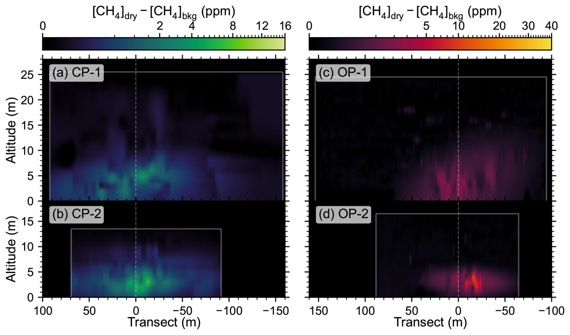
Figure 7 Kriged CH₄ enhancement fields from UAV-MPI for flights (a) CP-1 and (b) CP-2 and from UAV-NRCan for flights (c) OP-1 and (d) OP-2. The measured curtain extents are illustrated with boxes indicated by white lines, and the center of the curtain is indicated with a white vertical dashed line.

3.2.3 Gaussian plume inversion

The near-field Gaussian plume inversion (GPI) is applied by fitting Eq. (4) to the measured flux densities q_meas, calculated according to Eq. (5) and shown in the appendix (Fig.  C1). The GPI allows the modeled plume to be reconstructed in three dimensions. Therefore, for each measurement platform, we fit the measured data for one curtain but used the resulting plume model to reconstruct both curtains, for illustration purposes. The fit parameters for each curtain are summarized in Table 2. The modeled plumes obtained by fitting the far curtains (CP-1 and OP-1) are shown in Fig. 8, and the plumes obtained by fitting the near curtains (CP-2 and OP-2), are shown in Fig. 9.

Table 2 Fitting parameters for Eq. (4) obtained using the near-field GPI.

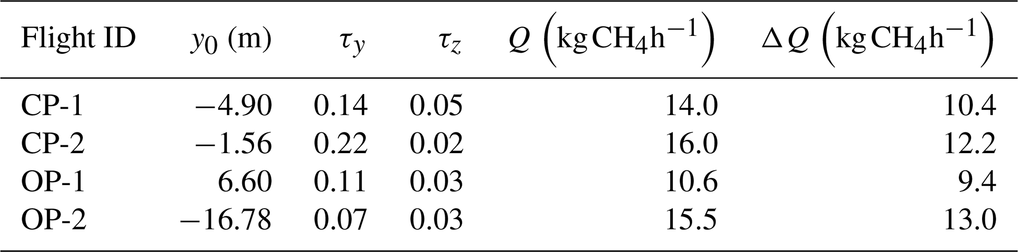
Figure 8 Modeled flux densities obtained from applying the near-field GPI to the far flux curtains (CP-1 and OP-1). The model results are shown for all four flux curtains, though the model parameters were obtained using only CP-1 and OP-1, indicated as Fit.

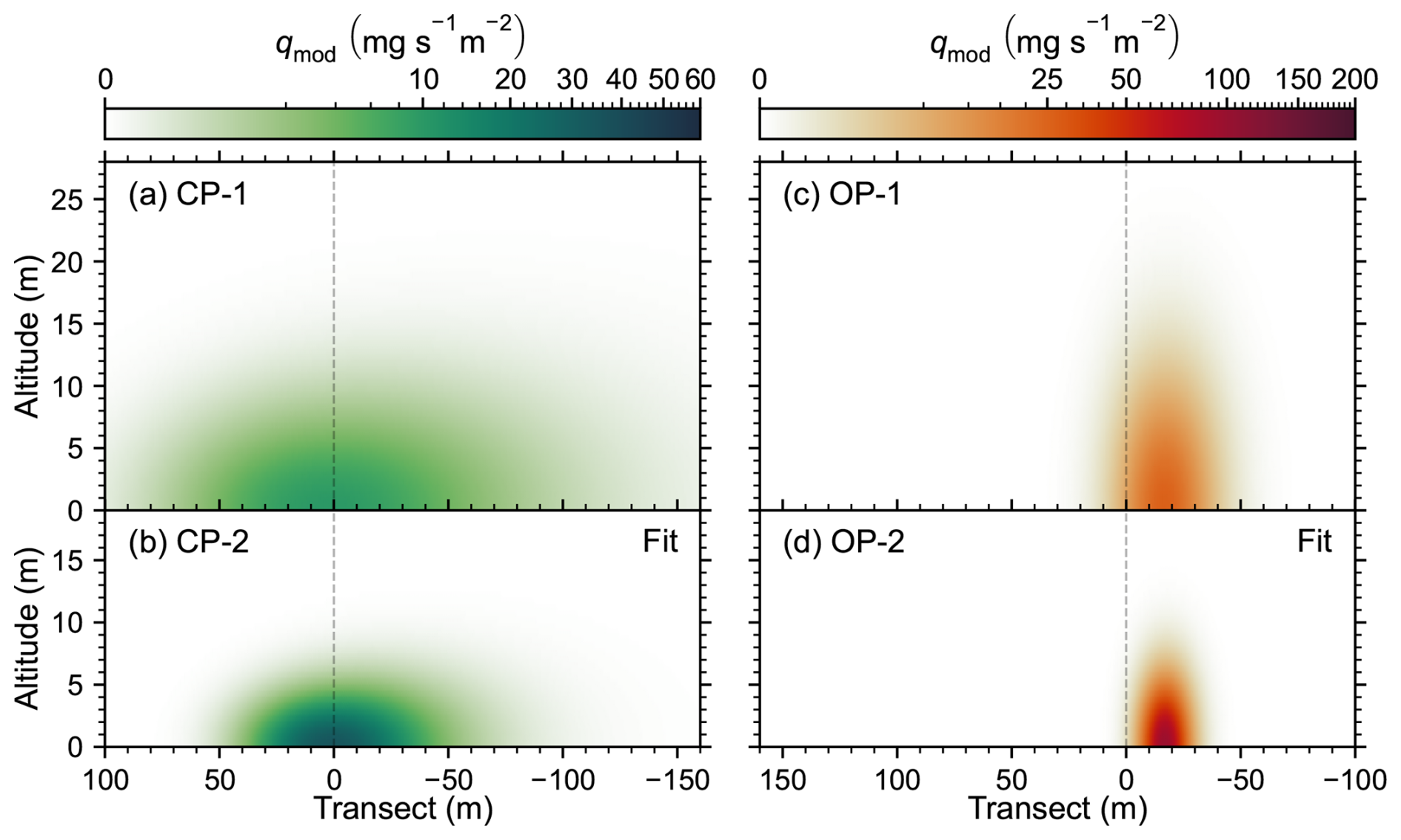
Figure 9 Modeled flux densities obtained from applying the near-field GPI to the near flux curtains (CP-2 and OP-2). The model results are shown for all four flux curtains, though the model parameters were obtained using only CP-2 and OP-2, indicated as Fit.

In all cases, the source height is fixed at h=0 and the remaining parameters are allowed to vary. We expected the plume to be centered close to y₀=0, in line with the prevailing wind direction. However, turbulence and variability in the instantaneous wind direction lead to non-zero values for y₀, ranging from −16.78 to +6.60 m. The deviations in y₀ are larger for the OP sensor compared to the CP sensor.

When fitting the far curtains (CP-1 and OP-1, Fig. 8), the shape of the modeled plume is similar for both the OP and CP systems, though the result obtained for the CP sensor appears more dispersed, attributed to the CP sensor's signal broadening effect. The results obtained when fitting the near curtains (CP-2 and OP-2, Fig. 9) show substantial differences in the shape of the modeled plume, with much broader apparent horizontal dispersion (τ_y) for CP-2 compared to OP-2. In this case, at just ∼ 80 m downwind of the source, the plume has had little opportunity to disperse and is highly influenced by turbulence and local eddies. At this distance, the difference in response of the CP and OP sensors is pronounced. Furthermore, we see that the perceived shape of the emission plume is strongly influenced by the response of the sensor. This suggests that application of prescriptive dispersion models that define the expected shape of a plume based on average local atmospheric conditions without accounting for the sensor response and the measurement duration, such as the Pasquill Stability Classes (Pasquill, 1961), are ill-suited for near-field measurements obtained by UAVs. However, in comparing Figs. 8 and 9, it is apparent that the capacity of the near-field Gaussian plume formalism to reproduce the shape of the plume in three dimensions remains limited, at least for downwind distances in the 80 to 150 m range with short observation times and atmospheric conditions similar to those presented here.

Comparing the emission flux estimates reported in Table 2, all values fall in the range from 10.6 to 16.0 kg CH₄ h⁻¹, in agreement within their respective uncertainties. The large error bounds, ranging from 74 % to 90 % of the corresponding flux estimates, are due to the large residuals between the Gaussian plume model and the measured data, indicating the Gaussian plume model does not adequately represent the measurement data. Though agreeing well within the prescribed uncertainty, we note that the difference between the estimated flux rates for the far and near curtains is smaller for the CP sensor compared to the OP sensor. We attribute this effect to the more gradual response of the CP sensor, which more closely resembles a smoothly varying Gaussian plume than the OP sensor.

3.3 Insights and lessons learned

Comparison between the methane concentration measurements for both UAV platforms shows that the OP analyzer often records sharper and larger CH₄ peaks, while the peaks are much smoother and damped for the CP analyzer. The OP analyzer may be preferable for plume tracking due to its higher sampling rate and lower latency compared to the CP analyzer. However, plume morphologies are discrete due to sharp peaks in OP, and rather smooth in the CP. Nevertheless, the quantification methods presented in this study regardless of analyzer type were able to produce consistent emission rate estimates for the seep, overlapping within their respective method uncertainty ranges. The estimated emission rates from all of these methods are provided in Fig. 10.

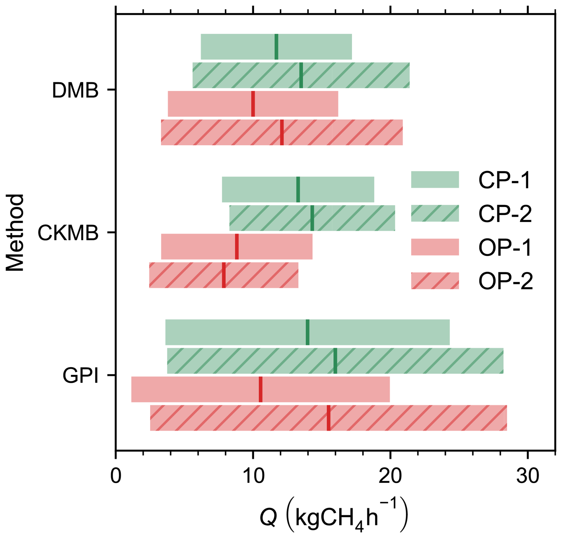
Figure 10 Emission rate estimations (Q) from different models and UAV platforms. Here, DMB, CKMB, and GPI denote Direct Mass Balance, Cluster Kriging Mass Balance, and Gaussian Plume Inversion approaches. Far curtains OP-1 and CP-1 are represented as solid red and green bars and near curtains OP-2 and CP-2 are represented with hashed red and green bars, respectively.

The application of DMB is straightforward and produces the most consistent emission rate estimates across both curtains and UAV platforms. However, adequate sampling density is essential, particularly in the vertical direction. Sparse sampling in the vertical direction can lead to large uncertainties and underestimation of the emission flux, especially when the plume center is missed (the uncertainties are estimated to be about 25 %). The uncertainties associated with the linear interpolations between transects are largely unknown and may be underestimated in this study. Further investigation is needed to rigorously quantify these uncertainties. The choice of the extrapolation method between ground and the first measuring height for DMB can significantly impact the resulting emission rate estimates. Collecting additional data while UAVs are on the ground may help to improve the extrapolation. The CKMB method provides excellent agreement in the emission rate estimates when comparing the far and near curtains for each UAV platform individually, and the interpolation uncertainty can be directly and conveniently quantified using covariance matrices. However, the variation between the platforms is greatest for CKMB compared to the other quantification methods. This is likely due to sensor response times and differences in flight execution: the OP platform utilized autonomous flight paths (resulting in regular sampling interval), whereas the CP platform was manually piloted (resulting in irregular sampling interval). Compared to DMB, the CKMB method is more complicated to apply and computationally more demanding as the curtain area increases. Additionally, fitting a variogram to the measured data usually requires optimizing the variance and length scales, which may not always converge (Andersen et al., 2021).

The near-field Gaussian Plume Inversion (GPI) generates emission rate estimates that are similar to the DMB and CKMB method estimates. Across all of the methods, there was less variation in the flux estimations for UAV-MPI (CP-1 and CP-2) compared to those for UAV-NRCan (OP-1 and OP-2). This variation in the OP sensor estimates was most notable in the GPI method, for which there was 38 % difference between the estimates for OP-1 and OP-2. Similar to the CKMB method, the GPI method tends to smooth the observed methane enhancements and widen the extent of the modelled plume both vertically and horizontally. When the morphology of the measured plume deviates strongly from a Gaussian shape, the GPI approach may be less suitable than other quantification methods, as the model cannot sufficiently explain the observation. This can prevent the optimization from converging or from finding the optimum parameters, as was reported in Andersen et al. (2021), even under relatively homogeneous conditions without any impact of topography and channel flow. In this study, deviation from the Gaussian plume shape is attributed to limited sampling time which cannot adequately represent time-averaged well-defined plumes, micro-topographical features that introduce additional disturbances, and channel flow rates that may distort the plume morphology (Shah et al., 2019; Allen et al., 2019). Therefore, over the seep area studied here with high-density sampling, mass balance approaches (CKMB and DMB) should be preferred when on-board wind measurements are available to avoid the large model – data mismatch as observed in GPI method. This can be to some extent mitigated by using both curtains simultaneously. Given the 3-D nature of the Gaussian plume model, it is also possible to fit the data from both the far and the near curtains simultaneously. For the CP sensor, fitting both curtains together leads to an estimated emission rate of 12.8±9.9 kg CH₄ h⁻¹, which is slightly less than the estimated flux rates for CP-1 and CP-2 individually. For the OP sensor, the combined estimate is 12.4±10.9 kg CH₄ h⁻¹, falling between the estimates for OP-1 and OP-2. GPI method can become practical whenever an on-board wind measurement is not available although this may lead to higher uncertainties. Additionally, the two-dimensional curtain flight patterns employed in this study may not be the optimum choice to retrieve the plume shape parameters required for the GPI method. Sampling strategies that use adaptive path planning to maximize the information gain in a limited time may be more suitable, as described in van Hove et al. (2026).

Overall discrepancies between applied quantification methods for each individual flights was on average 12 %, except for OP-2 where the difference was on the average 35 %. CMKB method estimations for OP sensor, compared to other two methods were lower especially for OP-2. This may be due to plume dynamics not being statistically stationary as indicated by the differences in CH₄ enhancements (see Fig. 7). OP-2 measurements do not show any enhancements above 6 m above ground level, while in CP-2, enhancements were observed even about 9 m above ground level. These differences affect the vertical interpolation of Kriging which resulted as smaller emission rate estimations compared to other methods. Furthermore, GPI estimation of OP-2 was almost double the estimation of CKMB. Since the CKMB method clusters the observational data as either enhanced or background, and interpolates these two clusters separately, the vertical extent of the predicted plume in CKMB compared to GPI method is smaller, hence the estimated emission rate. The observed differences (about 16 %) between mass balance methods can be attributed to the different interpolation schemes applied as well as UAVs sampling instantaneous plume dynamics rather than a static, theoretical representation of the plume. Moreover, these differences can also be partly attributed to the different flight strategies. While our analysis assumes the seep releases CH₄ directly into the atmosphere without significant interaction or advection within the water column, we acknowledge that water flow dynamics could potentially play a role in dispersing CH₄ prior to its atmospheric emission. Future investigations could benefit from measurements of water flow velocities and dissolved methane concentrations to quantify potential advection of CH₄ within the channel.

4 Conclusions

In this study, we evaluate several point source emission rate quantification methodologies using two UAV platforms equipped with methane analyzers, one open path (OP) and the other closed path (CP). Overall, the UAV-based methodologies presented in this study enable quantification of the emission rates from hard-to-access methane point sources that would otherwise be difficult to quantify.

Despite the differences in equipment and analysis methodologies used here and their associated uncertainties, the present work estimates that the methane emission rate of the investigated seep is in the range of 7.8 to 16.0 kg CH₄ h⁻¹ with an average value of 12.3 kg CH₄ h⁻¹ and standard deviation of 2.4 kg CH₄ h⁻¹ (see earlier seepage rate reported as 16.1 kg CH₄ h⁻¹ in Sect. 2.1).. Although this value only represents emissions during the active-layer thaw conditions, and does not reflect seasonal variations in emission rates, this average emission rate is significantly higher than biogenic sources. When compared to maximum daily biogenic CH₄ fluxes from permafrost landscapes (ranges approximately between 1.6–5 mg m⁻² h⁻¹, Friborg et al., 2000; Skeeter et al., 2022), emissions from this point source are equivalent to biogenic emissions from a minimum area of 2.5 km², pointing to the importance of identification, quantification, and inclusion of such emission sources in Earth-System models.

Appendix A: Custom temperature controller for Aeris Strato

The Aeris Strato CH₄ analyzer used on the UAV-MPI platform was customized with a thermally controlled enclosure to stabilize the cell temperature and reduce signal drift (see Fig. A1a). A thermal enclosure surrounding the measuring cell was added, including peltier elements for heating/cooling to keep the temperature within that enclosure stable (at 41 °C) using a temperature controller (TEC-1091, Meerstetter Engineering GmbH). This controller unit is directly powered by the analyzer board, minimizing system weight and complexity. We tested the performance of the analyzer against a calibration gas in a climate chamber. The calibration gas was routed through a coil-shaped steel tubing to equilibrate the gas temperature with the climate chamber temperature as much as possible.

Prior to testing the impact of the temperature controller, we observed large temperature fluctuations (±10 °C) within the analyzer cell under relatively stable conditions (see Fig. A1b). The TEC OFF test was conducted between 13:50 to 14:10 LT (black dashed lines in Fig. A1b). Although the climate chamber temperature was set to cycle between 10–15 °C every minute for about 20 min, the analyzer cell temperature was increasing throughout the test. This increase can be attributed to the low cooling efficiency of the thermally controlled enclosure and self-heating of the analyzer's cell. Subsequently, the temperature controller was turned on (TEC ON, 14:12 LT) and the instrument was allowed to warm up for about 30 min until the cell temperature was stabilized around 41 °C. The TEC ON test was conducted (red dashed lines in Fig. A1b) under the same climate chamber setup as TEC OFF test. The standard deviation of the cell temperature during TEC ON was calculated as 0.01 °C, whereas this was 1.62 °C during TEC OFF test. This was also reflected in CH₄ measurements (see Fig. A1c), the standard deviation during TEC OFF was 5.48 ppb (IQR 10.5 ppb), whereas during TEC ON this was 1.45 ppb (IQR 1.94 ppb). The improvement of the analyzer was also shown with Allan-Werle-plots (Fig. A1d). The instrument noise for longer averaging times is much smaller with the temperature controller unit compared to without one.

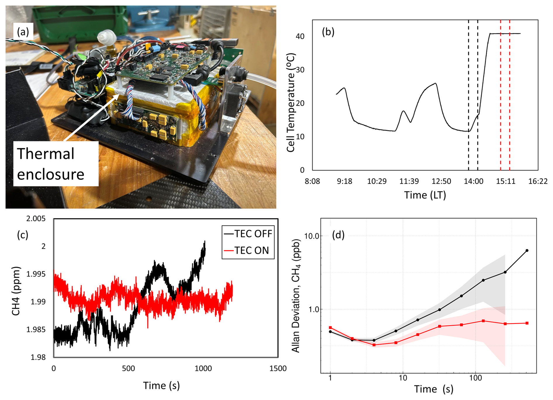
Figure A1 Customized Aeris Strato analyzer (a) showing thermally controlled enclosure wrapped around the measuring cell (b) recorded cell temperature of the analyzer during the climate chamber test, (c) measured CH₄ concentration with and without temperature controller (d) Allan-Werle-plots of both conditions. Here, red colors represent when the temperature controller unit was on (TEC ON) while black colors represent when the temperature controller was off (TEC OFF).

Appendix B: Timeseries data for measured flux curtains

Figure B1 shows the measured methane mixing ratios for all curtains from both UAV platforms.

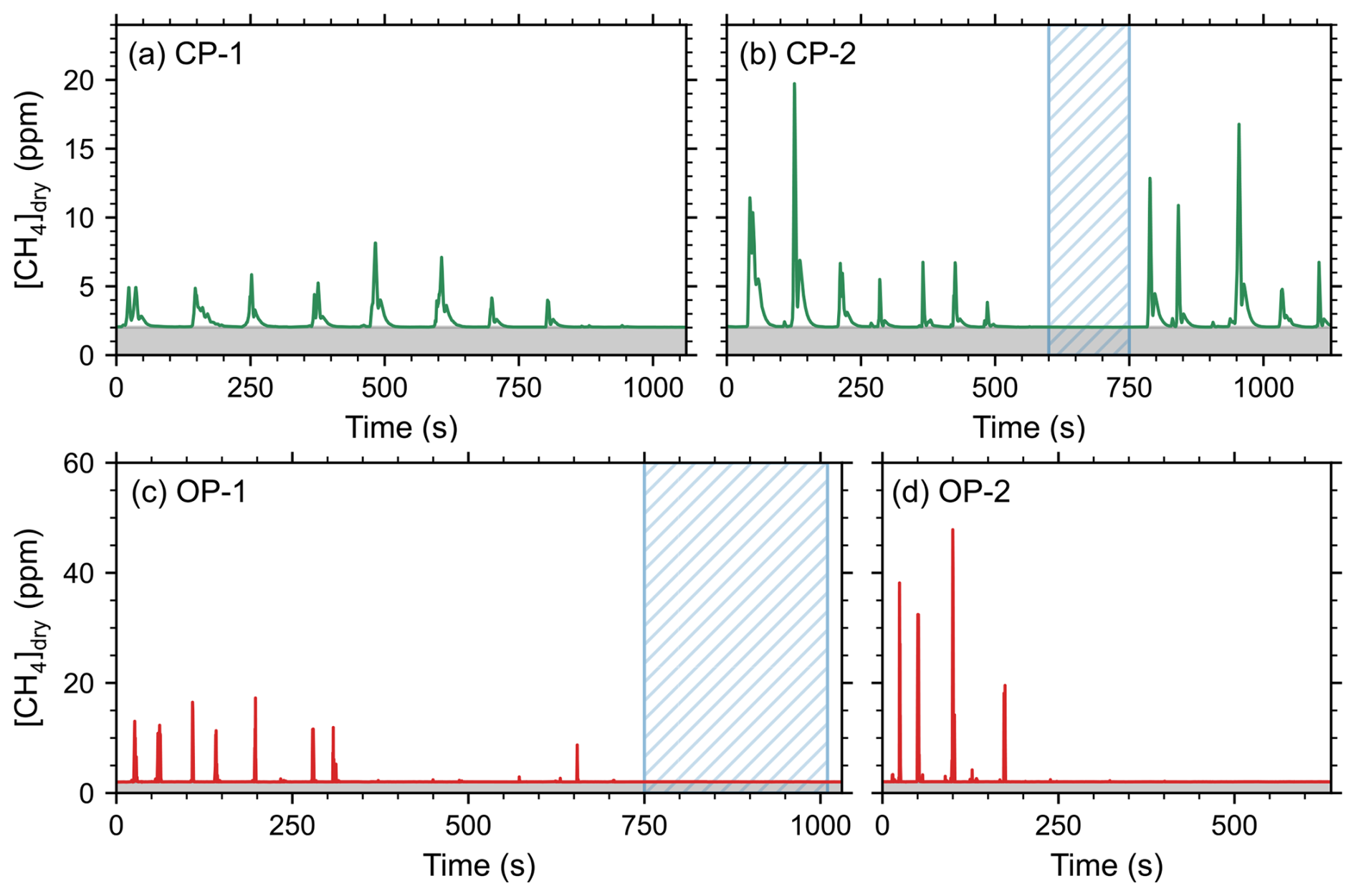
Figure B1 Measured methane concentration timeseries for the four curtain flights, labeled CP-1, CP-2, OP-1, and OP-2. The shaded regions indicate the background methane concentration, recorded as 2.0318 ppm for the closed-path sensor (a, b) and 2.0291 ppm for the open-path sensor (c, d). The background concentrations were estimated by averaging the measurements within the dashed region.

Appendix C: Flux densities used for Gaussian plume inversion

The calculated methane flux densities (q_meas) for all curtains from both UAV platforms are shown in Fig. C1.

Figure C1 Methane flux densities calculated from Eq. (5) (a, b). Flux density for the closed-path sensor at downwind distances of 163 and 87 m, respectively. (c, d) Flux density for the open-path sensor at 149 and 77 m downwind.

Appendix D: Wind speed and direction comparison

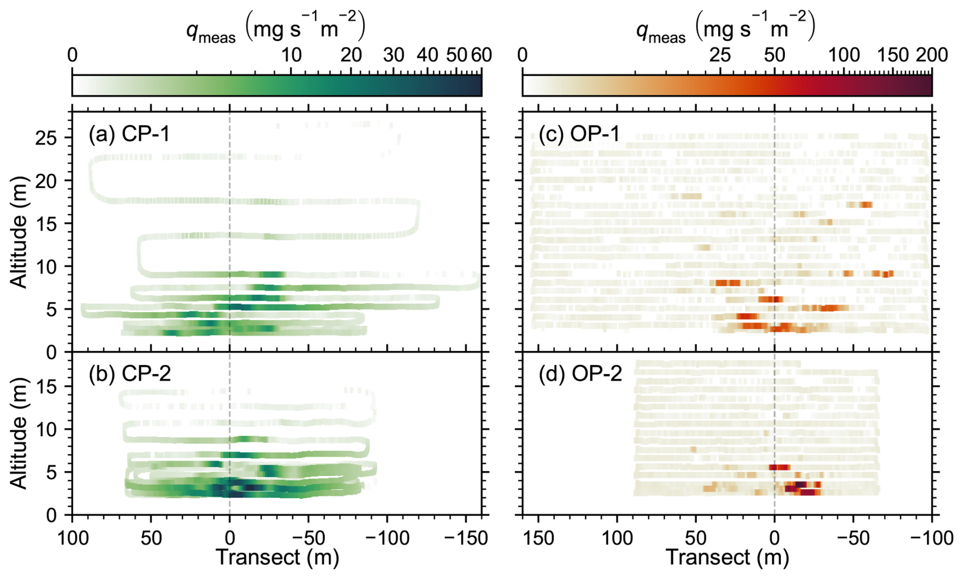
Figure D1 shows the measured wind direction and speed during all curtain flights and from ground-based sensors. Note that UAV-based wind measurements depart from the ground-based measurements as UAVs ascend during the curtain flight. The differences between the on-board wind measurements (CP-1 and OP-2, CP-2 and OP-1) are primarily due to spatial differences of the curtains (i.e. 150 vs. 80 m downwind distance from seep location) and different flight altitudes. This further demonstrates that all wind speed measurements are consistent throughout the measurement duration. We placed the ground-based sensors close to the seep location at two different heights, one at about 1.5 m (Windsonic4) above ground level and other (Gill Windultra) at about 2.7 m, while UAV-based anemometers were placed 0.67 and 0.75 m above the rotor plane in UAV-MPI and UAV-NRCan, respectively. Wind direction measurements agree well with the ground-based sensor after correcting the measurements from UAV-MPI and ground sensor (Windsonic4) north alignment.

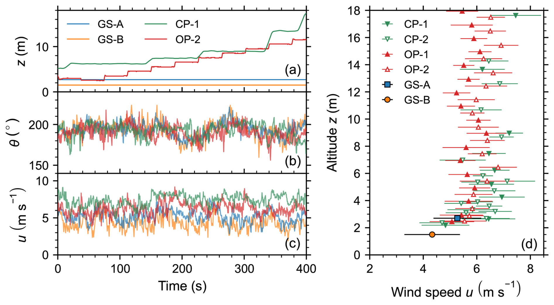
Figure D1 Comparison of wind measurements during CP-1 and OP-2 flights: (a) the altitudes of ground sensors and both UAVs, (b) wind direction measurements, and (c) wind speed measurements from both UAV platforms and ground sensors (GS-1: WindSonic4; GS-2: Gill WindUltra). (d) Wind speed measurements from all platforms during all four flights at different altitudes, where each symbol represents the mean wind speed and horizontal bars represent the standard deviations.