Assessment of the RFI environment in key passive microwave bands for Earth observation

Radio Frequency Interference (RFI) is spreading worldwide, affecting numerous Earth Observation (EO) instruments. Among these, microwave radiometers play an essential role, providing critical measurements for climate monitoring, weather forecasting, and numerous other applications. In order to plan for future satellite missions and fully exploit currently available measurements, it is crucial to study the contamination levels at bands where radiometers operate. This work presents the Earth Observation RFI Scanner (EORFIScan), an RFI detection system for EO products that combines multiple RFI detection techniques in order to reduce missed detections. This software has been used to assess several passive microwave bands from 6 up to 200 GHz, including both exclusive and shared bands. Analysis and validation of this method is presented for the year 2022. The resulting RFI probability maps show significant contamination in the bands up to and including 18.7 GHz; thus for the assessment, we mainly focus on bands from 6 to 18.7 GHz, where the most widespread contamination is found. A few brightness temperatures in the range of 350–400 K have been observed at 23.8 GHz and one at 36.5 GHz, which suggest the presence of man-made emissions. At higher frequencies, RFI contamination is not clearly visible in the analysed data. Comparisons with simulated radiances from a numerical weather prediction model are presented as a way to evaluate the RFI detection, finding that flagged observations are typically warmer than model simulations, as would be expected for RFI. It is clear from the results presented that RFI is already a concern for users at lower frequency passive microwave bands, and it is recommended that real-time monitoring systems are developed to keep an eye on the evolving threat of RFI in EO bands.

1 Introduction

Radio spectrum monitoring and enforcement actions are key to deliver radio protection and ensure that the different radio services operate in compliance with the in-force radio regulations and to secure an efficient and effective spectrum use, free from Radio Frequency Interference (RFI) (Pedro et al., 2022). Notwithstanding these essential actions, RFI is an inevitable consequence of the operation of radio systems, and it is a growing threat that has affected numerous Earth Observation (EO) satellite missions in recent years, especially passive microwave sensors (Draper, 2016b; Oliva et al., 2016; Piepmeier et al., 2014). These interferences vary widely in power level, radiation pattern, polarization, bandwidth, time duration, duty cycle, etc., and as a consequence there is no single algorithm that can optimally detect all levels and types of radiometric contamination (Querol et al., 2017).

The European Space Agency (ESA) and other space agencies rely on microwave radiometers for a wide variety of Earth Observation (EO) missions, operating in frequency bands from 1 to 700 GHz. RFI can negatively impact these radiometers in three different ways: High power RFIs can potentially damage the instrument, but have low occurrence probability; medium power RFIs cause data loss and gaps; and low power RFIs, mostly undetected, can distort scientific data, potentially compromising geophysical retrievals and weather forecasts.

It is thus of utmost importance to detect such RFI occurrences, not only to address their impact on the users' side, but also to support respective radio protection actions. However, instances of interference can vary widely not just in magnitude as mentioned above, but also in whether it is possible or appropriate to assign responsibility. Albeit the role of the International Telecommunications Union (ITU) in facilitating international coordination of radio protection actions, national administrations, by means of their National Regulatory Authorities (NRA), are responsible for overseeing the spectrum use and enforce the law in the territory under their jurisdiction. The bands typically used in EO missions fall into EESS (Earth Exploration-Satellite Service), including passive allocations with either exclusive access or shared access with active services. Service disruptions should always be reported to NRA who are responsible for conducting the required investigations and actions on the field to secure integrity of the spectrum so it can be effectively and efficiently used. In the case of exclusive access bands, clear violations, from the law enforcement standpoint, are easier to act upon. In case of shared access bands, the regulatory framework is still to be enforced. If the regulatory framework is enforced and service disruptions still occur, those findings are relevant in closing the loop for future enhanced spectrum policy, planning and assignment conditions. Comprehensive details about radio protection policies and practices can be found in (Pedro et al., 2022). There are numerous instances of the process to locate and shut down illegal transmissions ongoing, but new RFI sources appear constantly and the procedure to detect, attribute, and shut down illegal operators takes time.

In addition to clear violations of ITU regulations, many instances of apparent RFI come from legal operations in nearby bands or simply other users in a non-exclusive band. Furthermore, the spectral response of a radiometer can vary significantly from its specified bandwidth, and in this case apparent violations may be caused by radiometer sensitivity outside of the exclusive-use band due to being manufactured outside specified tolerances. Many space agencies now publicly provide measured spectral response functions (SRFs) for MW radiometers (SFCG, 2014) and it is a recognized best practice (English et al., 2020), but it is rare for heritage sensors and indeed most of the instruments studied here do not have measured SRFs publicly available. In other words, the cause of apparent RFI may be due to instrument design, illegal operators, or be a simple consequence of sharing a crowded part of the spectrum. No matter their source, satellite operators and downstream users need to address the inevitable presence of unwanted emissions.

Regardless of the source of RFI, and although the RF environment is constantly changing, it remains critically important for the planning of future EO missions to know the current status of contamination at bands of interest. For example, the L-band has been widely studied (Oliva et al., 2016; Bringer et al., 2018; Parde et al., 2011), and this has led to tangible changes in mission design and requirements for subsequent L-band missions. Nevertheless, the ESA RFI Monitoring & Information Tool (ERMIT) showed that the decreasing trend in worldwide contamination suddenly changed in 2024 when the Russo-Ukrainian war and the Myanmar civil war led to massive contamination in all observations over Europe and most of the South and South East Asia (ERMIT, 2025). C-band contamination was first discovered in AMSR-E measurements (Li et al., 2004). The presence of RFI in this band led to inclusion of an extra C-band channel on the follow-on AMSR2 mission for the purpose of RFI mitigation (Imaoka et al., 2010). RFI surveys conducted with different methodologies have only been conducted up to and including the 23.8 GHz band (Draper, 2018; Wu et al., 2020; Casey et al., 2022; Farrar and Jones, 2016), showing contamination in the 18.7 GHz band but not at higher frequencies. Quartly et al. (2020) reports RFI up to the 36.5 GHz band, albeit not widespread. Despite the best efforts of space agencies to predict the potential contamination issues of future EO missions, the RFI environment could change rapidly as services require more and more bandwidth, technology becomes more accessible and thus widespread, active services are aiming at higher frequencies, and the spectrum becomes more crowded with different users. Spectrum use, in the past, present and future, by Earth observation missions has been reviewed in Jorge et al. (2023).

The objective of this study is to survey RFI contamination in several key passive microwave bands from 6 up to 200 GHz using the same methodology, independent on the sensor characteristics (conical scan, across-track scan, …), in all bands commonly used by microwave radiometers using software developed under an ESA contract: the Earth Observation RFI Scanner (EORFIScan). This system is designed to be placed between the data generated from EO missions and the end users, such as the Numerical Weather Prediction (NWP) centres, with the goal of detecting and filtering RFI in order to avoid the assimilation of RFI-contaminated data. These new flags are appended to the original EO products. For this analysis, a comprehensive library of RFI detection algorithms is used, supported by external information and RFI databases. As the system analyses the incoming EO products, the results are stored in internal RFI databases that are used to improve future detection of RFI signals in the products. These databases show a picture of the RFI environment in each frequency band analysed. L-band is not analysed since EORFIScan is an upgrade of the Ground Detection RFI System (GRDS), which already surveyed this frequency band (Oliva et al., 2021), and frequency bands beyond 200 GHz the number of sensors working at these bands is reduced and RFIs are less likely to happen.

It is worth emphasizing that proper validation of RFI detection methods is difficult because no source of truth is available. Traditional metrics like a false alarm ratio are then hard to define, in contrast to a parameter like precipitation for which rain gauges offer a local measure of truth. In this study, RFI detection is assessed using simulations from an NWP model, following the idea that NWP model simulations provide information on the expected natural variability, which can be used as reference for RFI detection. This allows some validation of the methods, both instantaneously and in aggregate, but does not lead to specific conclusions on aspects like detection limits or false alarms. Furthermore, even an excellent RFI detection method will miss contamination that is within instrument or geophysical noise levels. This type of low-level RFI would be effectively undetectable on an instantaneous basis. Therefore, the lack of detection does not preclude the existence of RFI in a given band. This is especially true at higher frequencies where natural variability is larger due to more significant atmospheric signals.

This paper is structured as follows. Section 2 describes the system architecture, the RFI detection techniques utilized, and the threshold computation procedure, Sect. 3 shows the RFI maps of the passive microwave bands from 6 up to 200 GHz, which are discussed in Sect. 4. Section 5 describes the results validation, and Sect. 6 draws some conclusions.

2 Materials and Methods

This section presents a brief overview of the system architecture, describes which instruments were analysed during which time period, describes the RFI detection techniques applied in the analysis, and explains the procedure to compute the thresholds of each detection technique.

2.1 Instruments Used and Temporal Scope of the Analysis

In order to minimize the number of different instruments used to cover as many bands as possible, AMSR2 (Imaoka et al., 2010), AMSU-A (Mo, 1996), MWHS-2 (Zhang et al., 2012)) and AMR-C (Maiwald et al., 2020) were chosen. Table 1 shows the passive microwave bands under study and the bands and polarizations covered by each instrument. The numbers inside parentheses state which channels or bands each instrument has in each polarization in that band. AMSR2 provides observations at H (horizontal) and V (vertical) polarizations for all frequency bands, whereas the other instruments only measure one polarization. Cross-track scanners such as AMSU-A and MWHS-2 have polarization that shifts as a function of scan angle, with the polarization typically referred to as quasi-vertical or -horizontal (QV or QH) depending on the polarization at nadir. AMSR2, AMSU-A and MWHS-2 provide 2-D T_B observations per frequency band and polarization. AMR-C is, instead, a single-beam radiometer; therefore, it provides 1-D observations. Using these 4 instruments, all bands above L-band up to 200 GHz were covered. Note that the 18.7 GHz band is observed by two sensors (AMR-C and AMSR2), the 23.8 GHz is observed by 3 (AMR-C, AMSR2 and AMSU-A), and 89 GHz is also observed by 3 (AMSR2, AMSU-A and MWHS-2). This allows cross-validation between instruments. AMSR2 is the sole payload on GCOM-W, and is a one-off instrument. In contrast, the other instruments studied have flown or will fly on multiple satellite platforms. The analysis here uses AMSU-A from Metop-C, MWHS-2 from FY-3E, and AMR-C from Sentinel-6A.

Table 1 Passive microwave bands covered by this study, and instruments observing them. Parentheses state the channel number(s) that the instrument has in that band. Correspondence between channel numbers and band characteristics can be found in World Meteorological Organization (WMO) (2025).

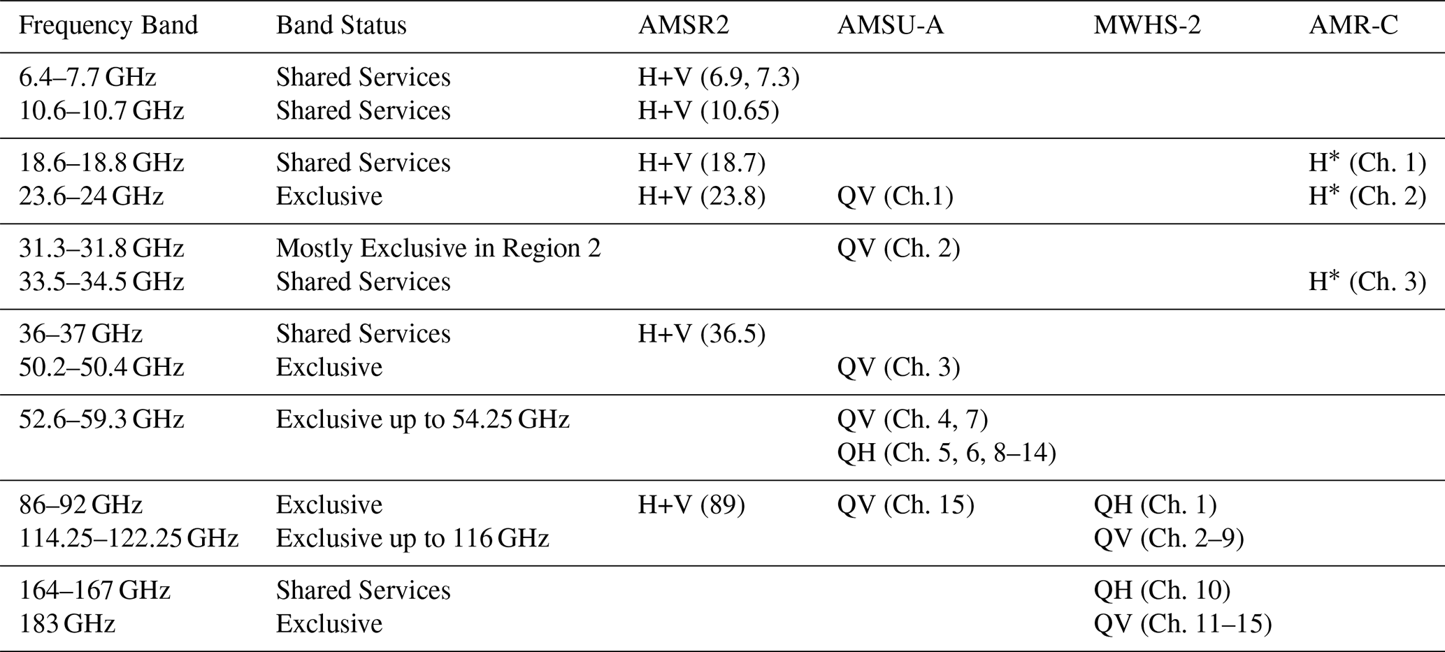
^∗ AMR-C observes at nadir using H polarization. V polarization is present in the instrument as back-up, since there is no difference between H and V observations when observing at nadir.

If the product contains the water fraction of each observation, pixels are labeled as “land” (water fraction lower than 5 %), “sea” (water fraction higher than 95 %), and “coast” (water fraction between 5 % and 95 %, and pixels 50 km up to away from the coastline according to CIA World Data Bank II; CIA, 1985). If the product only distinguishes pixels as land or sea, coast pixels are deduced as pixels up to 50 km away from the same coastlines database. Labels “sea-ice” and “storm/clouds” are added afterwards. In the case of AMSR2, sea-ice is detected using the ARTIST sea-ice algorithm (Spreen et al., 2008), which to the authors knowledge performs well in the Arctic marginal zone (Kern et al., 2019), and storms are obtained using the procedure from Draper (2016a). For AMSU-A, MWHS-2 and AMR-C, the k-means algorithm is used to separate “sea” into “sea-only”, “sea-ice”, and “storm/clouds”.

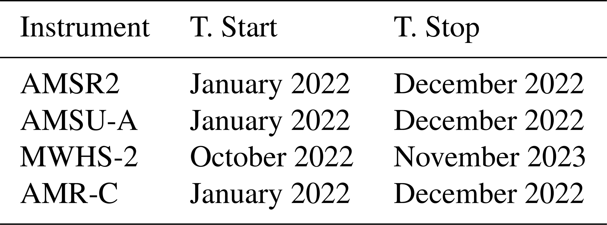
Table 2 shows the time span covered by the analysis, which tried to cover all 2022. However, MWHS-2 only provides observations for the 166 GHz band from October 2022 onward (in the case of satellite FY-3E, the first of the series FY that covers this band). In order to cover a similar period of time to be able to observe any seasonality, the time span analyzed from FY-3E covers 2023 instead of 2022.

Table 2 Time span for each satellite. The specified months are included in the analysis.

2.2 RFI Detection techniques

Multiple RFI detection techniques are applied to the observations with three progressive threshold levels. Different thresholds will therefore correspond to how strict the detection is, and how confident we are that the detections picked up actual RFI (referred later as “confidence level”). The flags for each frequency band are combined with a logical OR, so they keep the highest confidence level. By doing so, observations have 4 possible flags that can be encoded in 2 bits: no RFI flag, low confidence flag, medium confidence flag, and high confidence flag. The RFI techniques used in the analysis are the following:

• Intensity algorithm: An observation with brightness temperature T_B is flagged if T_B>α(λ), where α(λ) represents the threshold as a function of the latitude λ. We apply this detection algorithm to all assessed instruments.

• Polarization ratio: An observation with brightness temperatures T_H and T_V for H and V polarizations, respectively, is flagged if the polarization ratio P exceeds a threshold α(λ) that depends on latitude λ. We apply this detection algorithm only to AMSR2. The Polarization ratio is defined by Cavalieri et al. (1984) as:

  $$\begin{array}{}\text{(1)}& P={\displaystyle \frac{T_{\mathrm{V}}-T_{\mathrm{H}}}{T_{\mathrm{V}}+T_{\mathrm{H}}}}\end{array}$$

• Spatial Variability: An observation is flagged if the modulus of the components of the spatial variability (Gonzalez and Woods, 2018) is greater than a threshold α(λ) that depends on the latitude. For 2-D imaging, both components of the spatial variability are computed by doing the convolution of the data in the instrument reference frame (field of view number and scan number) with the matrices in Eqs. (2) and (3). We apply this detection algorithm to all assessed instruments.

  $$\begin{array}{}\text{(2)}& {\mathbf{H}}_{{\mathrm{SV}}_{\mathrm{1}}}=\left(\begin{array}{ccc}\mathrm{0}& \mathrm{0}& \mathrm{0}\\ -\mathrm{1}& \mathrm{0}& \mathrm{1}\\ \mathrm{0}& \mathrm{0}& \mathrm{0}\end{array}\right)\end{array}$$
  $$\begin{array}{}\text{(3)}& {\mathbf{H}}_{{\mathrm{SV}}_{\mathrm{2}}}=\left(\begin{array}{ccc}\mathrm{0}& \mathrm{1}& \mathrm{0}\\ \mathrm{0}& \mathrm{0}& \mathrm{0}\\ \mathrm{0}& -\mathrm{1}& \mathrm{0}\end{array}\right)\end{array}$$

  In the case of AMR-C, that is a 1-D instrument, the convolution is conducted with a vector composed of ten −1, a 0, and ten 1: $\langle \begin{array}{ccc}-\mathrm{1}\mathrm{\dots }-\mathrm{1}& \mathrm{0}& \mathrm{1}\mathrm{\dots }\mathrm{1}\end{array}\rangle$

• Image Enhancement: An observation is flagged if the modulus of the result of applying a high pass filter to the image (Gonzalez and Woods, 2018) is greater than a threshold α(λ) that depends on the latitude λ. To apply the high pass filter in 2-D images, the data in the instrument reference frame (field of view number and scan number) is convoluted with the matrix:

  $$\begin{array}{}\text{(4)}& {\mathbf{H}}_{\mathrm{HPF}}=\left(\begin{array}{ccc}-\mathrm{0.5}& -\mathrm{1.5}& -\mathrm{0.5}\\ -\mathrm{1.5}& \mathrm{8}& -\mathrm{1.5}\\ -\mathrm{0.5}& -\mathrm{1.5}& -\mathrm{0.5}\end{array}\right)\end{array}$$

  No useful equivalent has been found for 1-D sensors. We apply this detection algorithm to all assessed instruments except AMR-C.

• Generalized RFI Index: An observation is flagged if the generalized RFI Index ΔT_B[i] at a given frequency channel i is positive and larger than a given threshold α. The generalized RFI Index (Draper, 2018) is defined as the difference between observation T_B[i] and the expected value $\widehat{T_{\mathrm{B}}}\left[i\right]$):

  $$\begin{array}{}\text{(5)}& {\displaystyle }\mathrm{\Delta }{T}_{\mathrm{B}}\left[i\right]=T_{\mathrm{B}}\left[i\right]-\widehat{T_{\mathrm{B}}}\left[i\right]\text{(6)}& {\displaystyle }\begin{array}{rl}\widehat{T_{\mathrm{B}}}\left[i\right]& =a_{\mathrm{0}}\left[i\right]\\ & +\sum _{j\in \left\{f_C\left(j\right)\ne f_C\left(i\right)\left)\right)\right\}}\left(a_j\cdot T_{\mathrm{B}}\left[j\right]+b_j\cdot T_{\mathrm{B}}^{\mathrm{2}}\left[j\right]\right)\end{array}\end{array}$$

  The expected brightness temperature $\widehat{T_{\mathrm{B}}}$ is estimated using the brightness temperatures and their squared values of the other frequency channels j≠i weighted by the coefficients a an b, which are determined statistically by minimizing $min\left\{T_{\mathrm{B}}\left[i\right]-\widehat{T_{\mathrm{B}}}\left[i\right]\right\}$ for a large number of observations. If RFI is present, the observation ΔT_B[i] will be larger than the estimation $\widehat{T_{\mathrm{B}}}\left[i\right]$. Note that this technique assumes that the observations from other frequency channels are RFI-clean. Nonetheless, note that this is not always the case. This could lead to RFI contamination from other frequency channels leaking as false signatures in the desired channel. We apply this detection algorithm to all assessed instruments.

2.3 Threshold computation procedure

The EORFIScan has three threshold levels. Each is defined through a False Alarm Probability P_fa. The higher P_fa, the higher the number of detections, but their certainty decreases since the number of possible missed detections increases. In contrast, the lower P_fa, the lower the number of detections, but the higher the certainty of detection. From now on, the first case will be referred to as less strict and the latter as more strict in terms on how certain we are that a detection is not a false alarm. Thresholds might depend on geometrical or geophysical parameters such as the latitude or the incidence angle, the polarization or the terrain type. For instance, the physical temperature tends to be higher at low latitudes, and colder at higher ones, so it is expected the brightness temperature to follow this tendency, or in a similar way, the natural range of brightness temperatures over sea is different than the range over land.

Since one of the applications is to use the cleaned data to feed geophysical models, thresholds must be determined statistically and be model independent. Otherwise, the data used to feed models would only contain the data that already fit the models, preventing thus any improvement in these same models.

The time period used for the threshold computation has been determined empirically. For AMSR2, one week of each consecutive month of 2021 was used, to take into account the variability between seasons. For AMSU-A and MWHS-2, which have less dense data sampling, two weeks of each month were used. AMR-C data is even more scarcely sampled, so two full years (2020 and 2021) were used. Each instrument's thresholds have been computed separately using uniquely its own data.

The ideal procedure for setting the RFI detection technique thresholds is to first apply the RFI detection techniques to a large number of clean observations. Then, to estimate the probability density function f_X(x₁) for each frequency band, polarization, and surface type (e.g. land, sea, coast). Then, a threshold α defined by a given a priori probability of false alarm P_fa is found using Eq. (7) (Querol et al., 2017):

$$\begin{array}{}\text{(7)}& P_{\mathrm{fa}}=\underset{\mathit{\alpha }}{\overset{\mathrm{\infty }}{\int }}{f}_X\left(x_{\mathrm{1}}\right)\mathrm{d}{x}_{\mathrm{1}}\end{array}$$

The a priori probability of false alarm is defined as erroneously choosing hypothesis H₁ (RFI is present) when the true hypothesis is H₀ (no RFI is present), which can be formulated as $P_{\mathrm{fa}}=P\left(H_{\mathrm{1}}\right|H_{\mathrm{0}})$. The only exception to this procedure is the Generalized RFI Index, which first estimates the coefficients to compute the index, and then the thresholds are set to the PDF of the resulting error. In reality, it is impossible to exclude all samples contaminated with RFI, since this is actually the goal of the study. These samples modify the PDF used in Eq. (7). To minimize this effect, the strongest and most obvious contaminated samples and the nearby ones are excluded with a preliminary RFI screening method.

The function f_X(x₁) might not only depend on the random variable x₁, but also on the geometrical variables $y_{\mathrm{1}},\mathrm{\dots },y_N$ (latitude, longitude, incidence angle, azimuth angle, etc.). Ideally, the (N+1)-dimensional histogram of $f_X(x_{\mathrm{1}},y_{\mathrm{1}},\mathrm{\dots },y_N)$ would be computed and the threshold α would be computed for the desired P_fa for each N-dimensional bin $(Y_{\mathrm{1}},\mathrm{\dots },Y_N)$:

$$\begin{array}{}\text{(8)}& \begin{array}{rl}& P_{\mathrm{fa}}=\\ & \underset{\mathit{\alpha }\left(Y_{\mathrm{1}},\mathrm{\dots },Y_N\right)}{\overset{\mathrm{\infty }}{\int }}{f}_X(x_{\mathrm{1}},y_{\mathrm{1}},\mathrm{\dots },y_N|y_{\mathrm{1}}=Y_{\mathrm{1}},\mathrm{\dots },y_N=Y_N)\mathrm{d}{x}_{\mathrm{1}}\end{array}\end{array}$$

Estimating small P_fa values for all bins would require a huge amount of data, or else the threshold values for low P_fa values would be quite noisy. Instead, to simplify, it will be assumed that f_X depends at most on a single variable y₁ that stands for the most relevant geometrical variable. This variable is determined by inspecting the 2D histograms of x₁ against all possible y_n, taking into account that there might be no dependency. It also will be assumed that y₁ only changes the mean value of f_X with a deterministic function g(y₁):

$$\begin{array}{}\text{(9)}& f_X(x_{\mathrm{1}},y_{\mathrm{1}})=f_X(x_{\mathrm{1}}+g(y_{\mathrm{1}}\left)\right)\end{array}$$

Figure 1 (a) AMSR2 RFI pre-filtering map at 6.9 GHz and H polarization. Color axis shows the standard deviation of the high-pass filter value. (b) RFI Contamination maps observed by Draper (2018).

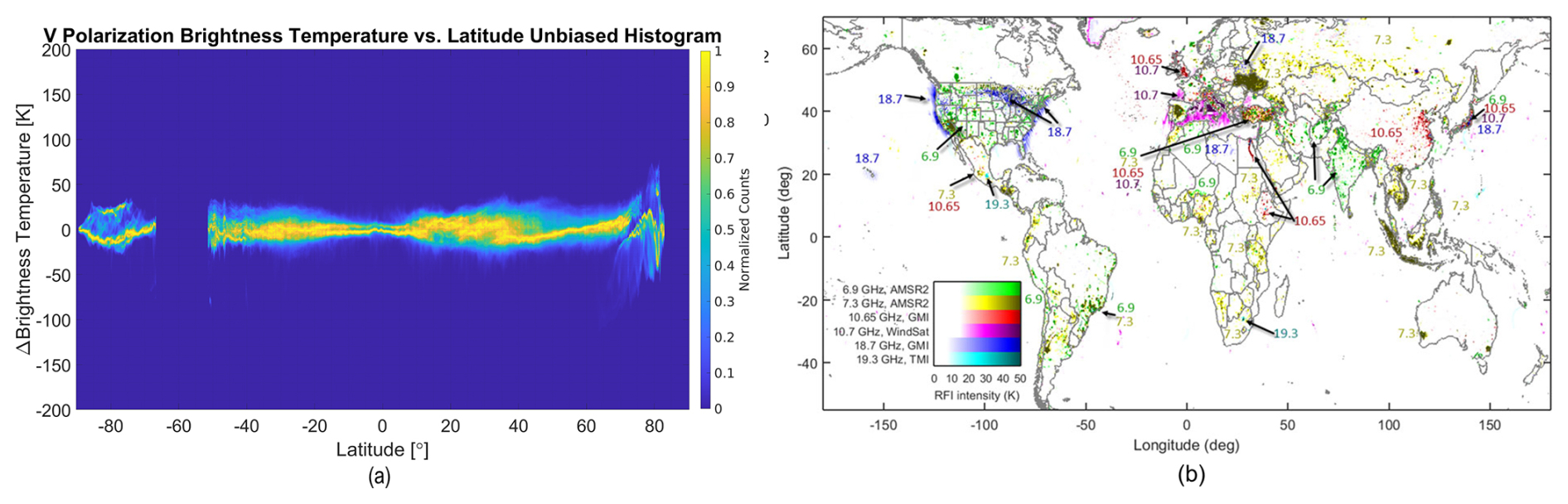
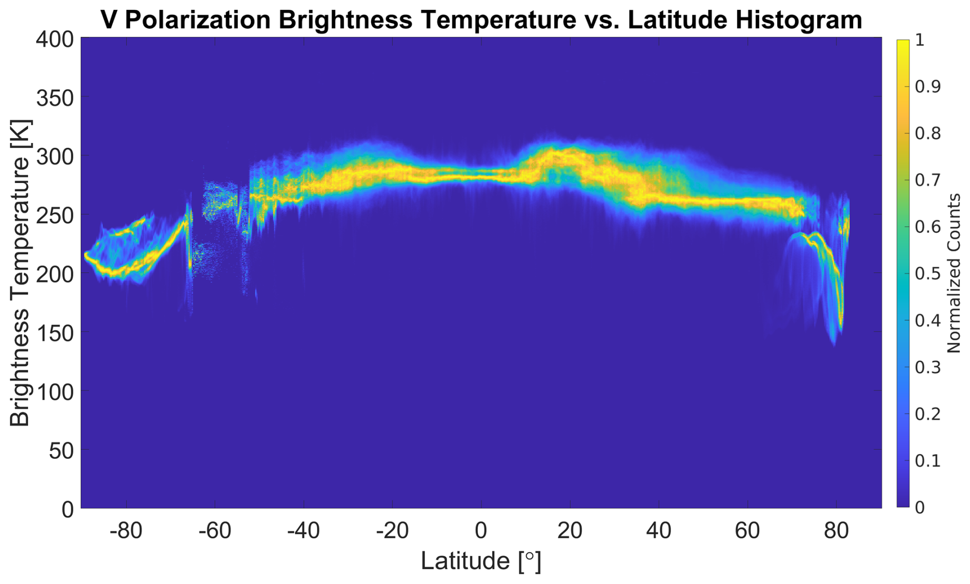
Figure 2 Biased 2-D histogram of the brightness temperature at 6.9 GHz V polarization in AMSR2 as function of the latitude.

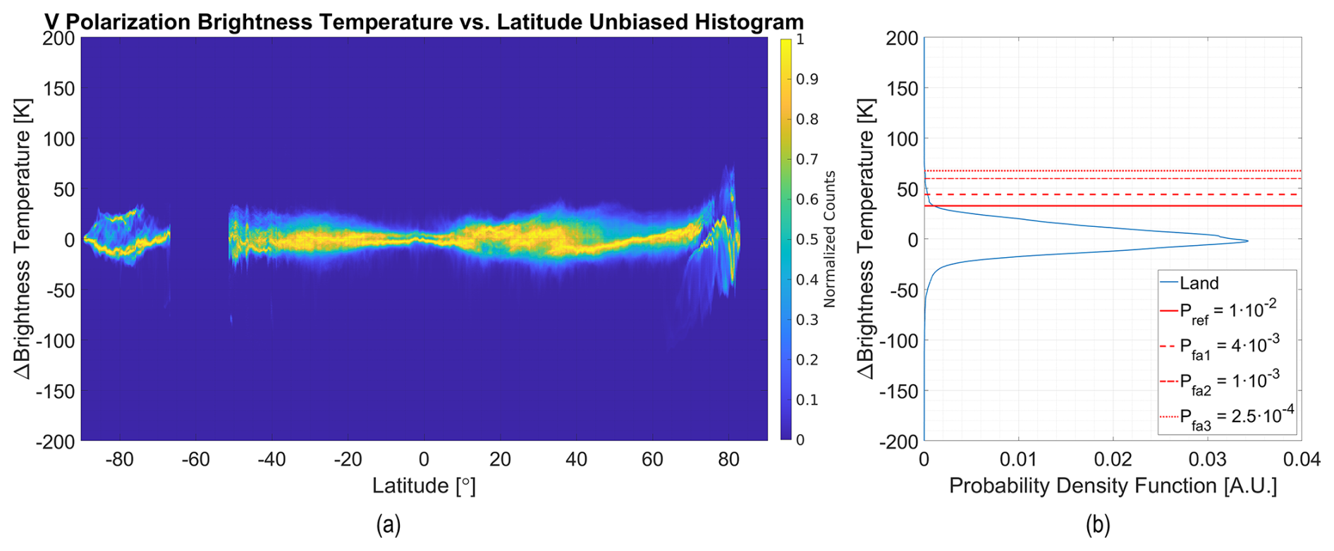
Figure 3 (a) Unbiased 2-D histogram of the brightness temperature at 6.9 GHz V polarization in AMSR2 as function of the latitude. The histogram is normalized in bins of 0.25° latitude. (b) Integrated 1-D histogram for the unbiased 2-D histogram in panel (a). The figure has been rotated and vertically aligned to match the integration of panel (a) along the latitudinal axis aligning their peaks.

The procedure for determining thresholds consists in first estimating g(y) so that f_x becomes the probability density function of a unidimensional random variable with deterministic dependency on the function g(y₁), then remove this dependency, and last compute the thresholds with respect this unidimensional random variable. The steps for this procedure are S.1 to S.9 described below.

S.1

First, the data from AMSR2, AMSU-A and MWHS-2 was pre-filtered for strong RFI contamination using the high pass filter from the Image Enhancement algorithm. AMR-C data are used without RFI prefiltering. To do so, the filter is applied and the results are collocated in cells of 0.5° × 0.5° in latitude and longitude. The standard deviation of each cell is computed, and the cells are classified according to their surface type (“land”, “sea-only”, “coast”, “sea-ice”, “cloud/storm”). For a given terrain type “land” and “sea-only”, cells are discarded if they are considered an outlier following the criteria ${\mathit{\sigma }}_X\ge \mathrm{median}\left(X\right)+\mathrm{4}\cdot c\cdot \mathrm{MAD}\mathit{\left\{}X\mathit{\right\}}$, where $\mathrm{MAD}\mathit{\left\{}X\mathit{\right\}}=\mathrm{median}\left(\right|X-\mathrm{median}\left(X\right)\left|\right)$ is the Median Absolute Deviation, $c=\frac{-\mathrm{1}}{\sqrt{\mathrm{2}}\cdot {\mathrm{erfc}}^{-\mathrm{1}}(\mathrm{3}/\mathrm{2})}$ (Leys et al., 2013), $\mathrm{erfc}\left(z\right)=\mathrm{1}-\mathrm{erf}\left(z\right)$ is the complimentary error function where $\mathrm{erf}\left(z\right)=\frac{\mathrm{2}}{\sqrt{\mathit{\pi }}}{\int }_{\mathrm{0}}^z{e}^{-t^{\mathrm{2}}}\mathrm{d}t$. Figure 1a shows the standard deviation of the high-pass filter in each cell for AMSR2 at 6.9 GHz H Polarization. Note how it matches the literature in Fig. 1b (Draper, 2018). Likely false positives due to sea-ice on the southern coast of Alaska, the Baltic Sea, and the Russian-Pacific coast are ignored, since they are “coast” pixels.

S.2

2-D histograms of each RFI detection technique (except the Generalized RFI Index), frequency band, and polarization are computed as a function of the available geometric parameters (latitude, incidence angle, etc.) to visualize which one has more influence. For instance, Fig. 2 shows the brightness temperature as function of the latitude. The dependencies found between thresholds and geometric parameters for each RFI detection techniques is mentioned in the list of RFI detection techniques in Sect. 2.2. The histograms are normalized in bins of the variable y₁ (the x-axis). In the case of the brightness temperature for ASMR2, the bins are 0.25° wide.

In the case of the Generalized RFI Index, once the coefficients a_i and b_i are estimated in Eq. (6), the 1-D histogram of the error in Eq. (5) is computed. In the case no geometrical dependencies are found, also the 1-D histogram is computed. Both cases jump directly to S.5.

S.3

The contribution g(y₁) is estimated as $\widehat{g}\left(y_{\mathrm{1}}\right)=\mathit{\{}x:f_X(x,y_{\mathrm{1}}\left)\text{ is maximum}\mathit{\right\}}$, and the unbiased 2-D histogram is computed as $\widehat{f_X}\left(x_{\mathrm{1}}\right)=f_X(x_{\mathrm{1}}-\widehat{g}(y_{\mathrm{1}}),y_{\mathrm{1}})$ as shown in Fig. 3a.

S.4

The 2-D histogram in Fig. 3a is integrated along the x dimension (latitude) and divided by the total area to obtain a 1-D Probability Density Function as shown in Fig. 3b.

S.5

The three desired thresholds α_i, i=1…3 (dashed lines in Fig. 3b) and a reference threshold α_ref (continuous line in Fig. 3b) are computed for a given set of $P_{{\mathrm{fa}}_i}$, i=1…3 and $P_{{\mathrm{fa}}_{\mathrm{ref}}}$ using Eq. (7). The reference false alarm probability is a high probability $P_{{\mathrm{fa}}_{\mathrm{ref}}}={\mathrm{10}}^{-\mathrm{2}}$ used to smooth the threshold function as will be shown later. The other false alarm probabilities are set to $P_{{\mathrm{fa}}_{\mathrm{1}}}=\mathrm{4}\times {\mathrm{10}}^{-\mathrm{3}}$, $P_{{\mathrm{fa}}_{\mathrm{2}}}=\mathrm{1}\times {\mathrm{10}}^{-\mathrm{3}}$, and $P_{{\mathrm{fa}}_{\mathrm{3}}}=\mathrm{2.5}\times {\mathrm{10}}^{-\mathrm{4}}$, respectively. In the case of 1-D histograms only the three thresholds α_i, i=1…3 are computed, and the procedure finishes here.

S.6

The distances between the thresholds to the reference threshold $d_i={\mathit{\alpha }}_i-{\mathit{\alpha }}_{\mathrm{ref}}$ are calculated.

S.7

The reference threshold α_ref(y₁) as function y₁ is computed in the 2-D biased histogram using Eq. (10), and is shown with a continuous red line in Fig. 4.

$$\begin{array}{}\text{(10)}& P_{{\mathrm{fa}}_{\mathrm{ref}}}\left(y_{\mathrm{1}}\right)=\underset{{\mathit{\alpha }}_{\mathrm{ref}}\left(y_{\mathrm{1}}\right)}{\overset{\mathrm{\infty }}{\int }}{f}_X(x_{\mathrm{1}},y_{\mathrm{1}})\mathrm{d}{x}_{\mathrm{1}}\end{array}$$

S.8

The threshold approximation function for the reference false alarm probability α_ref(y₁) is approximated with a M order polynomial, shown in Fig. 4 as a continuous green line:

$$\begin{array}{}\text{(11)}& {\mathit{\alpha }}_{\mathrm{ref}}\left(y_{\mathrm{1}}\right)\approx p\left(y_{\mathrm{1}}\right)=a_M\cdot y_{\mathrm{1}}^M+\mathrm{\dots }+a_{\mathrm{1}}\cdot y_{\mathrm{1}}+a_{\mathrm{0}}\end{array}$$

S.9

The threshold approximation function for each threshold level is defined as ${\mathit{\alpha }}_i\left(y_{\mathrm{1}}\right)=p\left(y_{\mathrm{1}}\right)+d_i$ and is shown in Fig. 4 as a dashed green lines.

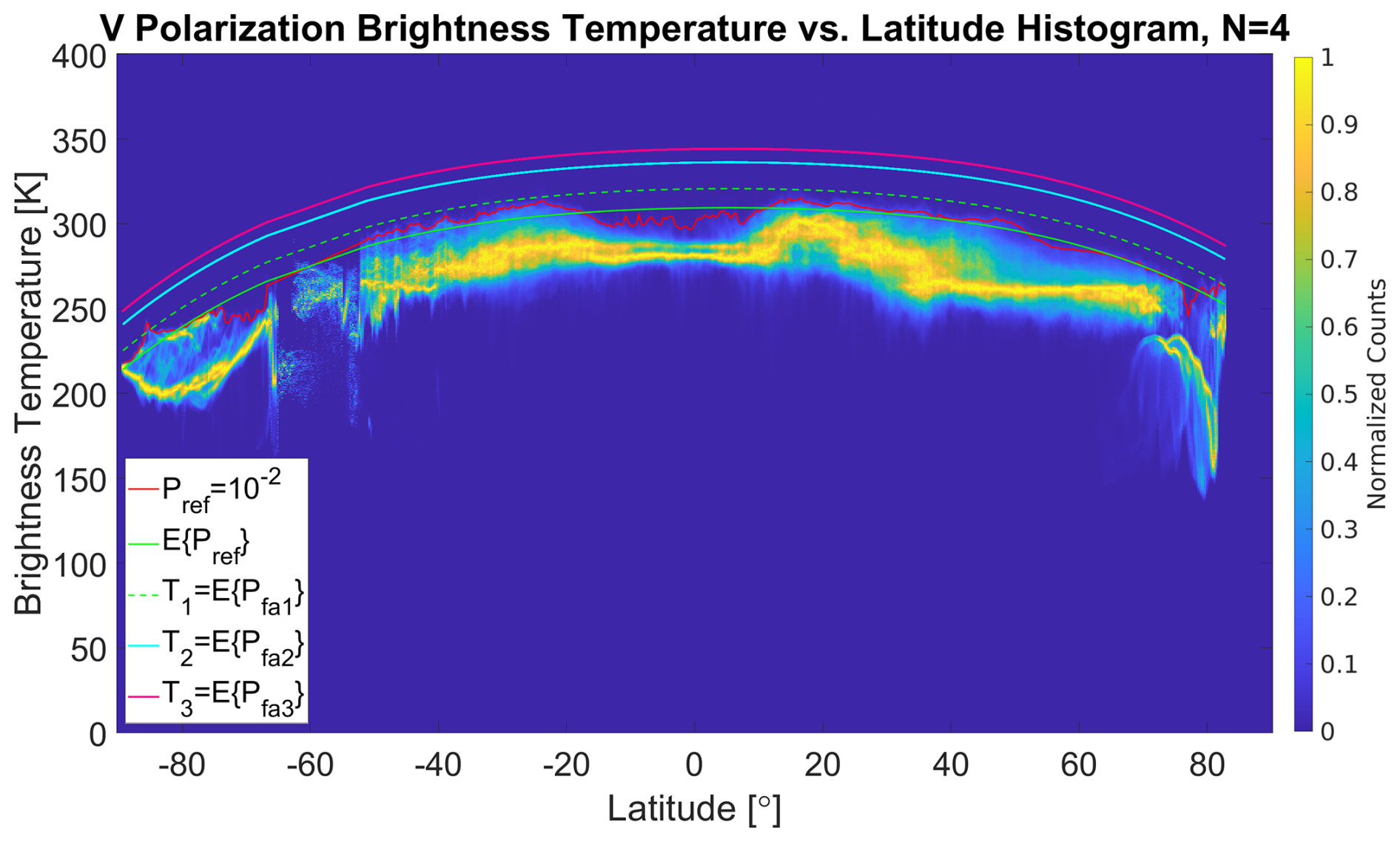
Figure 4 Biased 2-D histogram of the brightness temperature at 6.9 GHz V polarization in AMSR2 as function of the latitude, with the reference threshold α_ref(y₁) in red, the threshold approximation function for the reference false alarm probability in continuous green line, and the threshold approximation function for each threshold level in green dashed lines. The histogram is normalized in bins of 0.25° latitude.

If Eqs. (10) and (11) were used to directly compute α_i(y₁), a large dataset would be required since $P_{{\mathrm{fa}}_i}$ are small, and small datasets will imply excessively noisy estimations. Still, large datasets will not ensure that two polynomial approximation functions α_i(y₁) do not cross each other. The procedure described here reduces the amount of data needed, and ensures that threshold approximation functions do not cross each other, and therefore increasing false alarm probabilities always ensures a less strict threshold as defined at the beginning of this subsection.

Note that this subsection focused on the probability of false alarm and does not mention the a priori probability of missed detections P_md. Calculating P_md requires knowing the statistics on the RFI sources. These statistics are scarce, vary over time, have been conducted in particular frequency bands (not necessarily generalized to other bands), and barely include low power RFIs, the ones more likely to be miss detected. As a consequence, this computation is not possible or may be inaccurate.

Note that since no ground truth is available, it is not possible to estimate the a posteriori probability of false alarms or the a posteriori probability of missed detections.

3 Results

In order to evaluate the status of the RFI environment, RFI probability maps are used. Neither AMSR2, AMSU-A or MWHS-2 data is gridded, so EASE2 grid with 25 km spacing has been used for the database. Observations are assigned to the closest grid point. Then, the probability of RFI is calculated at each grid point as $P_{\mathrm{RFI}}=D/O$, where D is the number of RFI detections, and O is the total number of observations.

The maps are computed for each month along the temporal scope of each sensor analysis using both ascending and descending data, and both H and V polarization (if available). In the following, we present maps of mean RFI probabilities generated from these monthly maps, with the aim to highlight areas that are consistently flagged as RFI-affected. While these average maps may not capture more transient events that are only present during certain times, they provide a representative overview of the main affected areas. Average maps are a good trade-off between showing RFI contamination and mitigating false alarms.

Furthermore, after discarding measurements potentially affected by sun glint, observations over 350 K were stored along with their latitude, longitude and date per each frequency band. Then, they were grouped into clusters using k-means method.

Figures 5 to 9 show mean RFI probability maps for selected channels from the four instruments considered, covering the frequency range 6.9 to 183 GHz. Maps from AMSR2 have been prioritized over AMSU-A since two polarizations are available, and consequently the resulting maps are less noisy. Furthermore, the higher the frequency, the noisier the maps, since the spatial resolution is higher, the atmospheric effects on the T_B become more intense, and the atmospheric contributions are less smooth than the land or sea dynamics particularly because cloud and precipitation sensitivity generally increases with frequency.

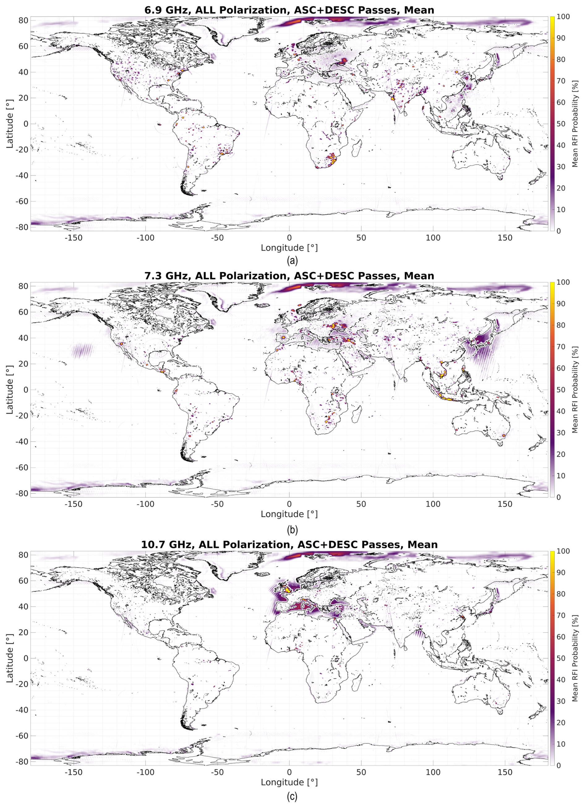
Figure 5 RFI Probability maps for: (a) 6.9 GHz (AMSR2), (b) 7.3 GHz (AMSR2), and (c) 10.7 GHz (AMSR2).

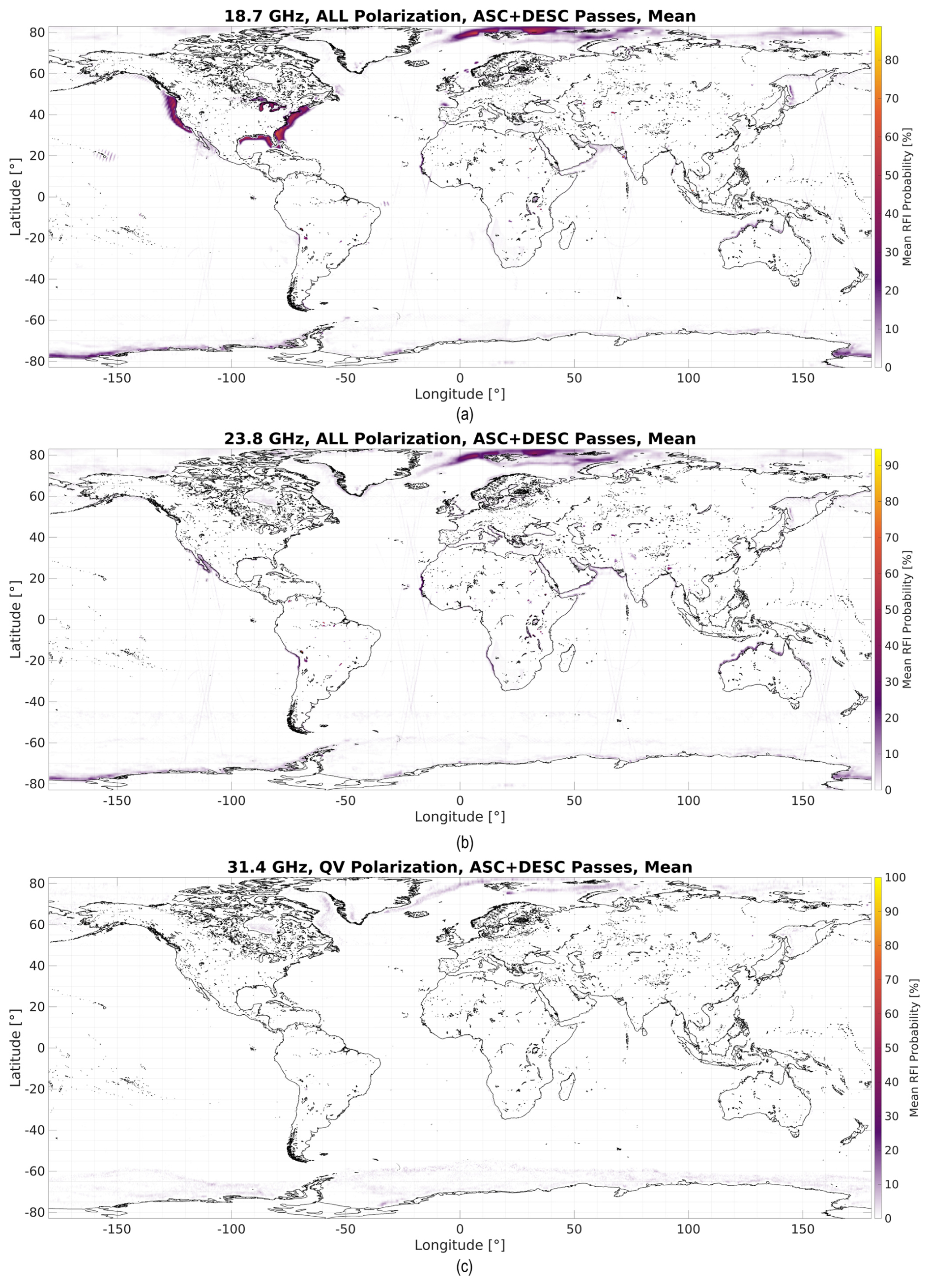
Figure 6 RFI Probability maps for: (a) 18.7 GHz (AMSR2), (b) 23.8 GHz (AMSR2) and (c) 31.4 GHz (AMSU-A).

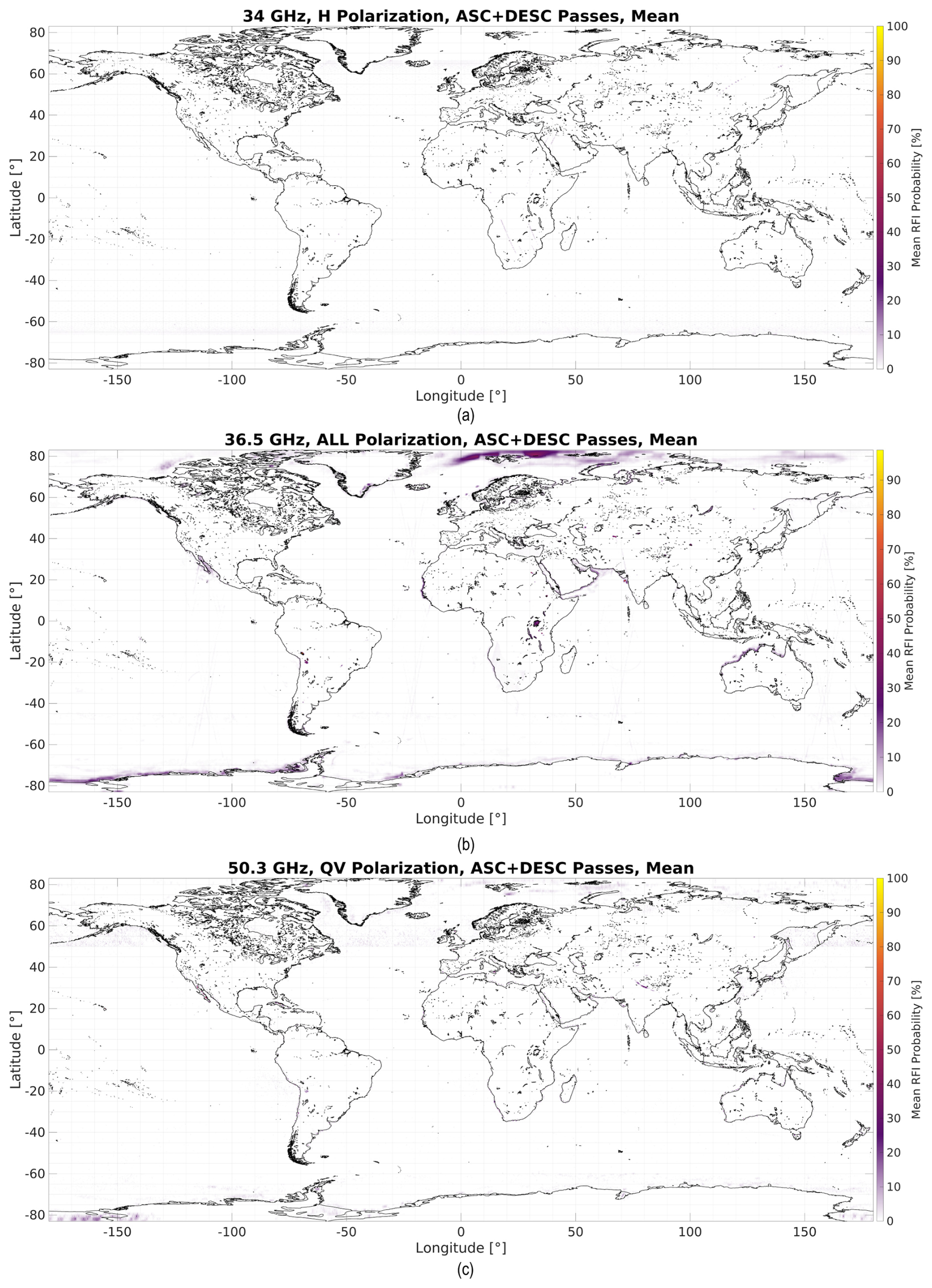
Figure 7 RFI Probability maps for: (a) 34 GHz (AMR-C), (b) 36.5 GHz (AMSR2), and (c) 50.3 GHz (AMSU-A).

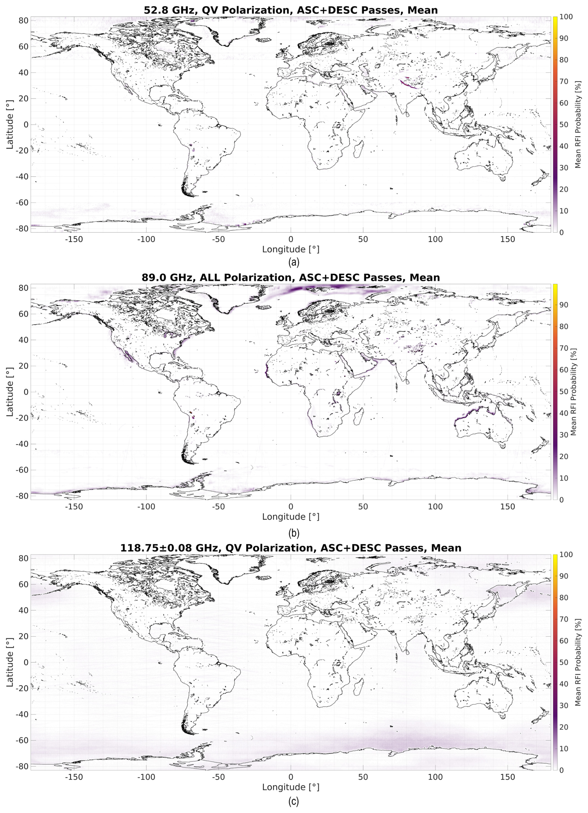
Figure 8 RFI Probability maps for: (a) 52.6–59.3 GHz (AMSU-A), (b) 89 GHz (AMSR2), and (c) 118 GHz (MWHS-2).

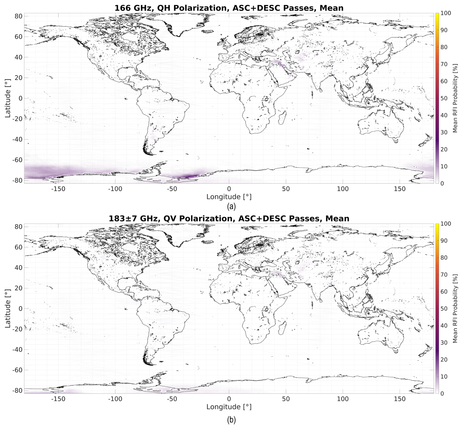
Figure 9 RFI Probability maps for: (a) 166 GHz (MWHS-2), and (b) 183 GHz (MWHS-2).

4 Discussion of the Identified RFI Environment

The 6.4–7.7 GHz band is not exclusively allocated for passive applications and therefore passive sensors cannot claim protection. This regulatory framework can be linked to the significant contamination documented previously (Draper, 2018; Wu et al., 2019, 2020). It is separated into the 6.9 and 7.3 GHz sub-bands. At the 6.9 GHz sub-band contamination is widespread in the US, and India. Some contamination is scattered in South America (with a denser detection area in Brazil), in Africa (with a denser detection area in South Africa), Europe (note the dense detection area over Ukraine and the detection from possible oil rigs in the North Sea), and the sea contamination in the Yellow Sea in front of China probably due to marine traffic. Point sources of 6.9 GHz contamination over sea had previously not been identified in the literature. In the 7.3 GHz sub-band contamination is present in all populated continents. Both North and South America show a few scattered detections, with strong detections in Central America. Europe also shows a few RFI sources, mostly in the North Sea due to oil rigs, and a large contaminated area over Ukraine. The Middle East is heavily contaminated in Turkey and Syria, with some contamination seen in Saudi Arabia. Indonesia and Thailand show strong signatures across their entire areas due to a telecommunication service using this band. Some isolated RFI sources can be seen in the rest of Oceania. Also note the reflection of geostationary satellite signals over the sea near Japan, in the Mediterranean Sea and the Atlantic Ocean near Europe, and in the Pacific Ocean between Hawaii and the US.

Only a part of the 10.7 GHz band is exclusive for passive services (10.68 to 10.70 GHz), whereas AMSR2 has a nominal bandwidth from 10.60 to 10.70 GHz. RFI contamination is mostly present in Europe due to the reflection of geostationary TV broadcast satellites over the sea (Scanlon et al., 2025). The reflections are seen as stripes following the descending orbit direction. The same signatures can be seen as descending stripes in the Bay of Bengal near the coast, which were not observed in previous analyses. Some strong signatures can be seen in the UK, and some contamination is visible along the Nile River, in Nigeria, on the east coast of China, Mexico, Middle East, Central and Western Europe, Australia and widespread in Japan and Turkey.

The 18.7 GHz frequency band is not exclusive for Earth Observation, but despite this the RFI contamination maps are relatively clean. RFI contamination is found on the US coast, also including Hawaii. No other regions seem to be contaminated. However, the analysis focused on 2022; since then, strong contamination has been observed by the recent Compact Ocean Wind Vector Receiver onboard the International Space Station (COWVR-ISS) instrument (Brown and Morris, 2024). It is true that COWVR-ISS has a larger bandwidth than AMSR2, and the detected RFIs could be out of the AMSR2 bandwidth. This fact plus a growing presence of contaminated areas makes an RFI detection and mitigation system increasingly attractive at this frequency band.

Figure 10 AMSR-2 RFI Probability maps centred at the Norwegian coastline for: (a) 6.9 GHz, (b) 7.3 GHz, (d) 18.7 GHz, and (e) 36.5 GHz; and (c) Oil Rig distribution near the Norwegian coast in 2022 (NOD, 2024).

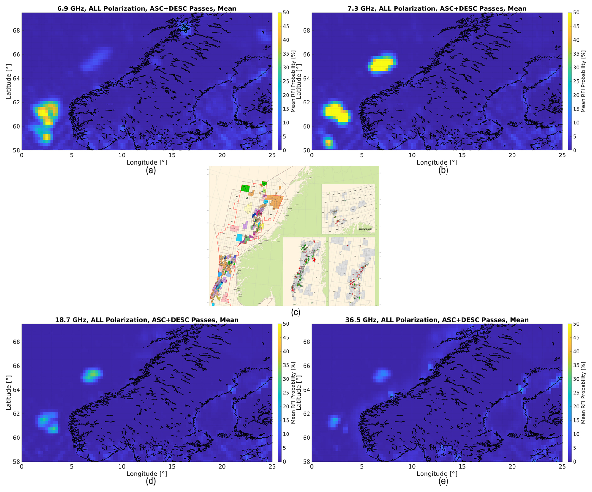
One area where we can zoom in is near the Norwegian coast in the North Sea and Arctic Ocean, where several spots of contamination at different bands can be observed. They closely match the location of the 2022 oil rig maps observed in Fig. 10 and it seems reasonable to view this as causal. These signatures are only observed by AMSR2. They are also visible at 6.9, 7.3 and 36.5 GHz, but not at 10.7 GHz, and 89 GHz (see Sect. 3). A possible explanation could be that the RFI Index technique is causing false positives due to the coefficients associated with certain bands. Bands where RFI is erroneously detected (tentatively 18.7 GHz) are explained by the coefficients in a and b corresponding to the T_b of the channels where the RFI is present being negative, contributing positively to the RFI Index (see Eq. 5). On the contrary, in bands that do not show this “cross-contamination” effect, the coefficients in a and b corresponding to the T_b of the channels where the RFI is present is positive, contributing negatively to the RFI Index. Figure 10 shows that the upper RFI detected area at 7.3 GHz and the lower RFI detected area at 6.9 GHz seem to be “cross-contaminating” the 18.7 and 36.5 GHz maps, since patterns have similar shapes. It could be the opposite way, but it is less likely that an oil rig is transmitting at 36.5 GHz, since commercial radio links are common at 6.9 and 7.3 GHz bands.

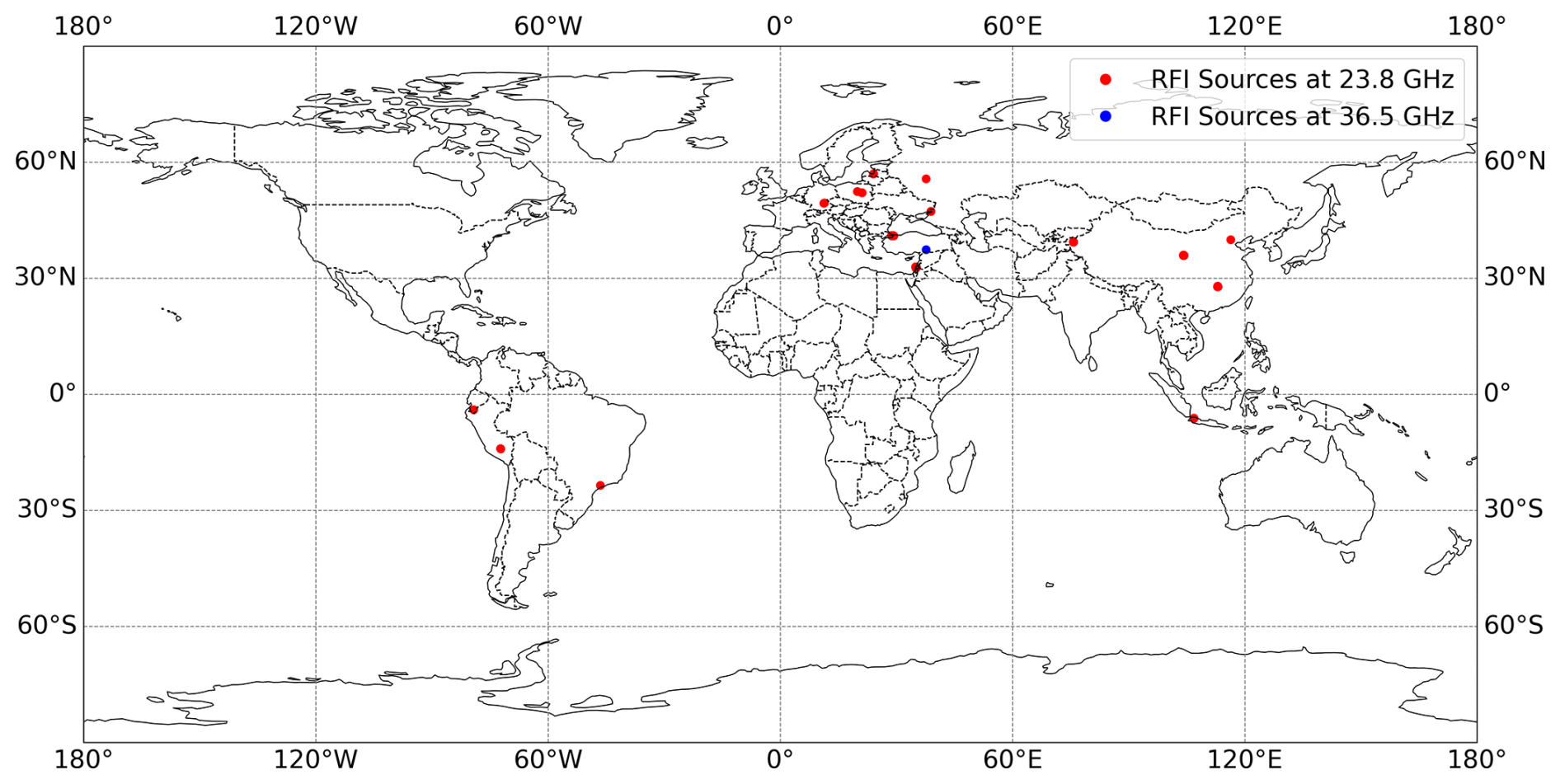
Figure 11 Map showing the location of all RFI at 23.8 GHz (red), and at 36.5 GHz (blue).

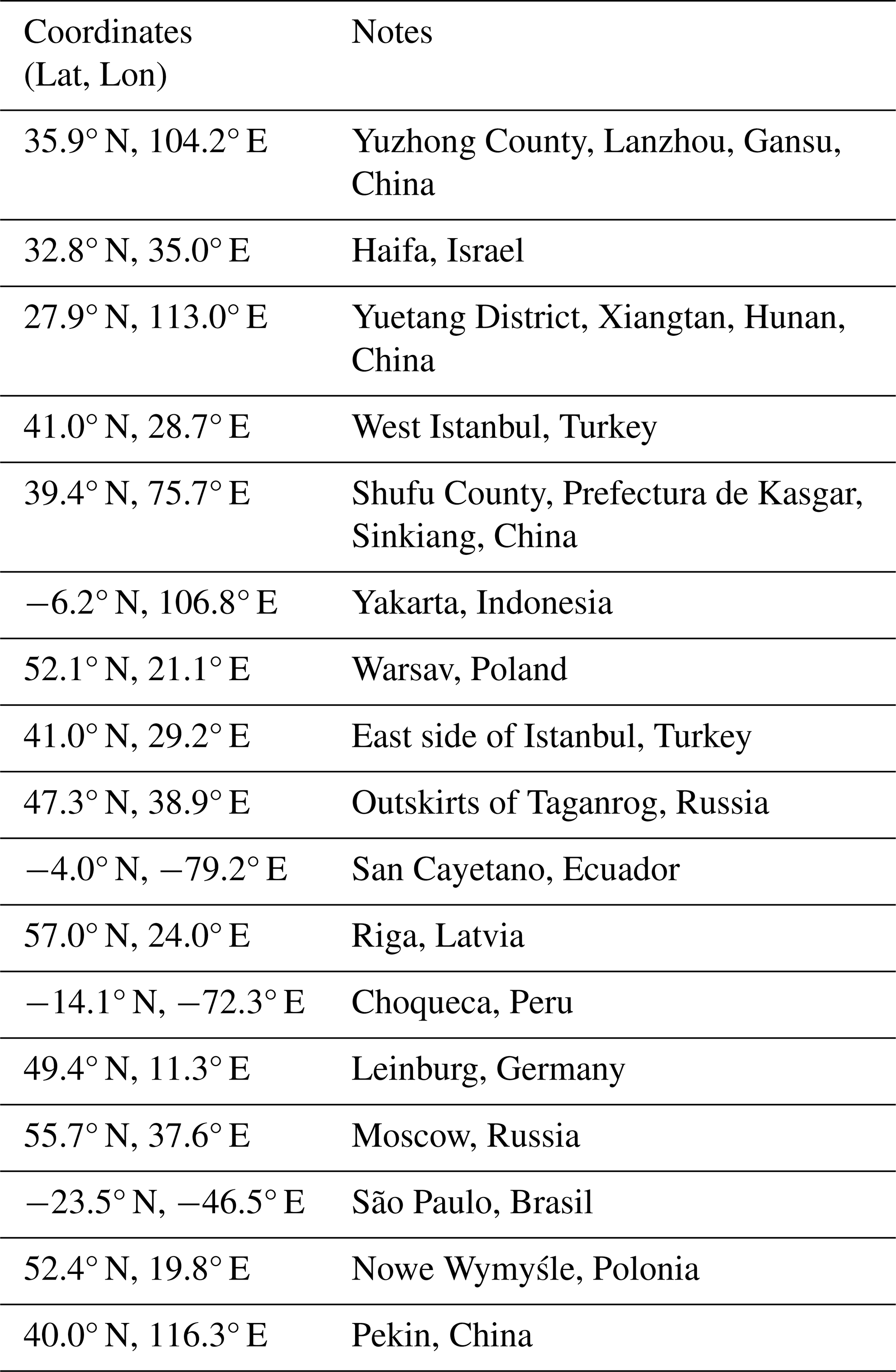
The 23.8 GHz frequency band is exclusive for passive services, but the deployment of communication services for 5G services in the nearby band 24.25–27.5 GHz might cause RFI contamination in this band. This band was identified for use by 5G in 2019 (Ookla, 2023). Analysis of the AMSR2 measurements at 23.8 GHz highlighted instances in which the measured brightness temperature was between 350 and 400 K which indicates presence of RFI. Some of those observations are suspected to be caused by sun glint. These measurements were scattered along a constant latitude that changed from month to month, and matched the regions prone to sun glint shown in (Wentz et al., 2021) and Sect. 3 of (Kazumori et al., 2016) whose latitude also change along the year. Some of these observations even showed abnormally high values compared to the surrounding area in the higher frequency bands. These observations were discarded from the analysis. The rest of those observations over 350 K were grouped in clusters and are listed in Table 3. The largest cluster of RFI signatures is located in Yuzhong County, Lanzhou, Gansu, China. These observations are, to our knowledge, the first confirmed detection of RFI in the 23.8 GHz band. The COWVR-ISS also reported RFI in this frequency band (Brown and Morris, 2024), but since the instrument's bandwidth is 75 MHz larger than the allocated band for passive observations, it is not possible to ensured if it is an in-band or out-of-band emission. Adjacent channels include mobile and fixed communications, and amateur communications. All RFI observations have been located in a World map in Fig. 11. These detections are not observed in the RFI Probability maps since the number of contaminated observations is proportionally low to the total number of observations collocated to a cell. Furthermore, the smaller antenna swath makes adjacent cells not to contain any contaminated observations, and therefore they do not show the typical “bump” shape. As consequence of both, the effect of these observations in the maps can not be distinguished from the detection noise.

Table 3 Centroid coordinates of each cluster of RFI signatures at 23.8 GHz band, sorted by number of observations.

The 31.3–31.8 GHz is exclusive for passive services in region 2, but no clear signs of RFI contamination can be seen except than false positives in already previously mentioned areas such as sea-ice missed classifications and coastal up-welling areas. The band from 33.5–34.5 GHz is shared but results do not suggest man-made RFI contamination. RFI has been found in this frequency band with COWVR (Brown and Morris, 2024), but the larger bandwidth of COWVR (1975 MHz) also covers part of the adjacent bands. Therefore, these reported sources cannot be confirmed as in-band.

The 36–37 GHz band is shared with other services. RFIs have been reported in this frequency band in November 2018 caused by a radar facility in Roi Namur in the Kwajalein atoll, Marshall Islands. The RFI signal only affected the gain of the Sentinel-3 instrument, and the radiometric data quality was not affected (Quartly et al., 2020). No clear RFI signatures were detected in the considered dataset. AMSR2 data showed 1 single observations in 2022 over 350 K which could not be linked to sun glint effects. The only remaining observation is located at 37.41° N, 37.61° E in Araban, Gaziantep province, Turkey. This RFI observation has been located in a World map in Fig. 11.

At higher frequencies, there were no clear detections of RFI signals in the considered dataset, regardless of whether the bands are exclusive or shared. The signatures shown in the maps seem to respond to geophysical signatures rather than RFI contamination due to their large extension, location, and variability throughout the year. Most bands show false detections at the sea-ice borders as a result of missed classifications in both hemispheres, even after using a sea ice concentration algorithm that performs well in the ice marginal zone (Kern et al., 2019). Threshold could have been adjusted to reduce the false positives in the ice edges, but it would had come at the expense of misdetections in this area. Although not many RFI are expected here, some ships cross this area and their presence should not be neglected. False detections can also be seen at the borders of the Greenland ice sheet, or in the Himalayan mountains. Many coastlines, such as the Mauritanian coast, the Angola-Namibia coast, the Chilean-Peruvian coast, the north-west coast of Australia, the Yemen-Oman coast, the Somalia coast, the Baltic Sea coastline, the Yellow Sea coastline, and the California coast show a high RFI probability in many frequency bands (such as 18.7, 23.8, 36.5, or 89 GHz) and instruments. Capone and Hutchins (2013) shows correspondence between these areas and the so-called upwelling regions of the ocean, of which the four main ones are the Chilean-Peruvian coast, the California coast, the Angola-Namibia coast, and the Mauritanian coast. The water anomaly observed by this effect in the Canary and California currents can reach 4 K after long time averaging and could explain the detection in these areas (Gómez-Ocampo et al., 2018; Benazzouz et al., 2014). For analogous reasons to the sea ice edge false alarms, softening the thresholds might result in misdetections in marien regions such as the Yellow sea of the seas around Japan. Other false positives are observed in South America and Africa can be seen in all frequency bands such as the Lakes Titicaca and Poopó. The RFI probability changes over the year with a stable decreasing trend until mid-year, when it starts to increase again. This could be caused by a reduction on the water level during summer until the rainy period in winter.

5 Results Validation

NWP models compare millions of observed radiances with model-simulated radiances every day as part of the data assimilation procedure. For microwave radiances at ECMWF, this process employs the RTTOV-SCATT radiative transfer model (Geer et al., 2021), simulating radiative effects from the surface, atmospheric gases, clouds, and precipitation – a so-called all-sky simulation. The observed radiance (O) is compared to the model's short-range forecast simulation of the observation, known as the model background (B), interpolated in time and space to the observation location and with the same viewing geometry. This is the first step of the assimilation of the observations, which will subsequently lead to updated model fields. In addition to offering information to update the model state, analysis of departures between observations and model (O−B) can be instructive for monitoring the quality of observations themselves. It is worth noting that in this study the full spatial resolution of radiances are analyzed (i.e. with no averaging applied), in contrast to typical pre-processing of observations before assimilation at ECMWF that includes averaging (superobbing) for most microwave data.

Simulations of the NWP model background do not include artificial sources. The background thus represents a realization of a pristine RF environment, one with natural sources of emission only. Analysis of departures can therefore aid in the identification and quantification of RFI sources, as the natural range of O−B variability is known very well in most cases. For example, over the ocean at low frequencies that are primarily sensitive to SST, O−B variations are typically within about 1 K. This provides a tight constraint on expected behavior, allowing abnormal radiative signals to stand out as likely contamination. Instantaneous departures can show these anomalous scenes, but the real power of NWP-based monitoring is in the aggregate, with signals able to emerge even in noisy sampling over many days and weeks. Crucially, RFI should manifest as a positive O−B signal only, whereas other mismatches between the model and observations should be distributed between positive and negative departures. For example, a misplaced cloud in the model background will show up at a cloud-sensitive frequency band as a positive blob next to a negative one, whereas a region of RFI should be overwhelmingly positive. Even if RFI is coincident with cloud and precipitation, the large amount of sampling afforded by NWP-based analysis means that these signals should still be clear in time-averaged maps and histograms.

In this validation analysis, only results from AMSR2 low frequency channels are presented, covering March and October of 2022. This is to focus on frequency bands in which significant contamination was found. Fuller analysis can be found in the technical report from (Duncan and Bormann, 2024), and comprehensive analysis of AMSR2 performance in the ECMWF system can be found in Kazumori et al. (2016).

5.1 Definitions, Screening, and Instantaneous Departures

Here we define the departure with inclusion of a bias correction term, as calculated by the variational bias correction scheme used within the data assimilation system (Auligné et al., 2007). This is a method of removing persistent sources of bias between observations and model, including overall instrument bias against the model plus terms for angular and atmospheric thickness components among others. Inclusion of the channel-dependent BC term here is important for analyzing AMSR2, which has roughly 2–5 K mean biases against the ECMWF model at several channels (Duncan et al., 2024). This should also aid in isolating signals of contamination rather than bias. The departure is defined:

$$\begin{array}{}\text{(12)}& D_{\mathrm{BC}}=(O-B)-\mathrm{BC}\end{array}$$

To illustrate what can be seen in the departures, Fig. 12 shows AMSR2 observations at 18.7V, the model background simulated values, and the difference. East of the United States' east coast is a long frontal region of cloud and precipitation, resulting in positive and negative departures side-by-side. In contrast, the area around Florida shows relatively weak but persistent positive departures of roughly 5–10 K, consistent with a reflected geostationary broadcast signal. In this way, RFI contamination can be identified by eye in O−B fields.

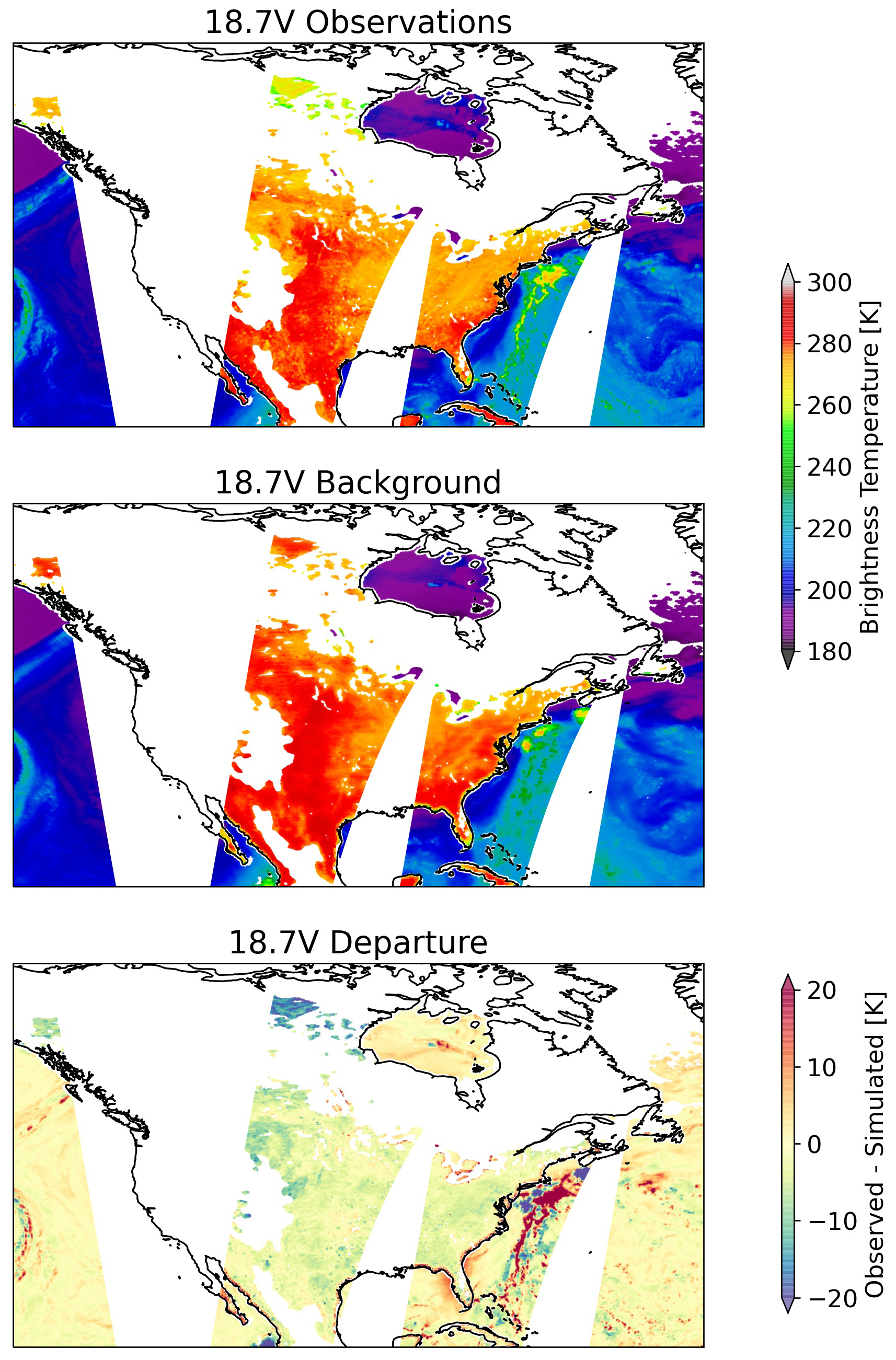
Figure 12 Observed radiances (top), model background equivalents (middle), and background departures (O−B; bottom) from AMSR2 18.7V on 2 October 2022 over North America.

However, the fidelity of model-simulated radiances is not the same everywhere and it is therefore necessary to introduce some screening of departures for statistical analysis. For example, microwave radiances over ice-free oceans have very well-modeled surface emissivities at the frequencies discussed, whereas more challenging surfaces such as sea-ice, high orography, and snow-covered ground have much poorer emissivity modeling. Certain regions are thus screened out of the validation analysis in order to exclude areas of known model bias or deficiencies in the forward modeling. This is why frozen surfaces of Canada, high orography of the Rocky Mountains, and some coastal scenes are not shown in Fig. 12. This data selection essentially follows the screening rules for microwave imagers assimilated at ECMWF (Geer et al., 2022). For more details on the data selection, see (Duncan and Bormann, 2024).

RFI sources are spectrally narrow in most cases and should therefore be distinct between radiometry bands. This is important for departure-based RFI detection because model assumptions and radiative transfer modeling will be very similar at nearby frequencies. Consequently, a forward model error such as an erroneous surface emissivity will manifest similar at nearby frequencies whereas RFI will not. Figure 13 shows departures from the three lowest frequency bands on AMSR2 at V over Western Europe. The left panels show all departures, while the right panels show only points that EORFIScan flagged as likely RFI. As the figure presents descending nodes of the GCOM-W orbit and AMSR2 scans in the forward direction, it is possible to see reflected RFI from geostationary sources, particularly over sea at 10.65V in the Bay of Biscay, the North Sea, and in parts of the Mediterranean. It is also clear that some surfaces over land are simulated better than others, with larger model biases apparent over complex surfaces and some artefacts along coastlines. Regardless, several point sources of RFI are evident through localized positive departures over both land and sea, most evident at 6.9V in the North Sea, Luxembourg, and southern Spain, at 7.3V at different sites in the North Sea and Italy, and then very strong sources at 10.65V in the UK and Italy. Most of the clear examples of RFI in the left panels are identified by EORFIScan in the right panels. One possible exception is 7.3V contamination in Italy where despite both 6.9V and 10.65V RFI in the vicinity, the much stronger departures at 7.3 GHz suggest likely RFI here.

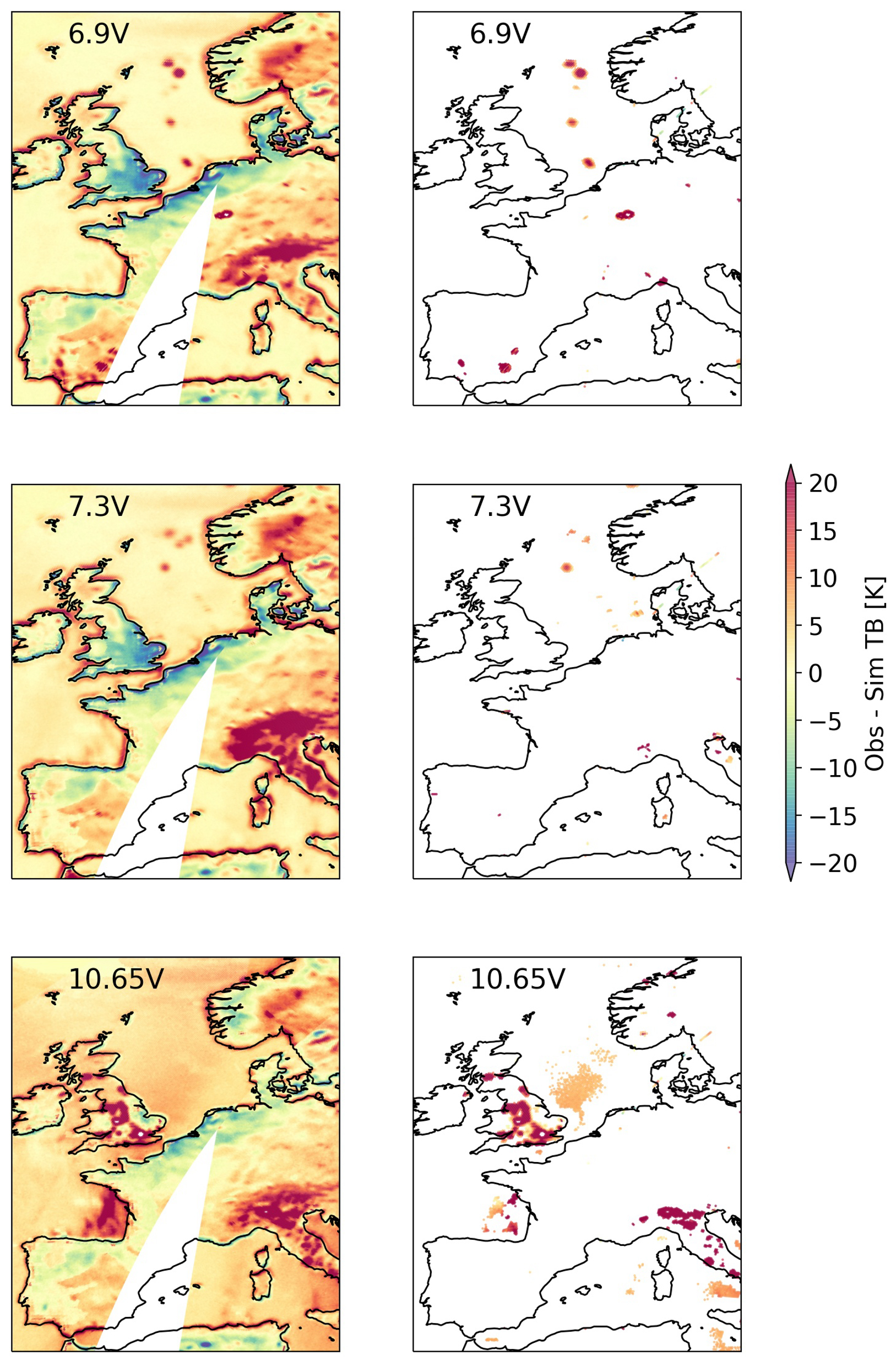
Figure 13 Departures for AMSR2 channels 1, 3, and 5 (all V) on 2 March 2022 over western Europe. The right column only shows departures identified by EORFIScan as likely contamination.

5.2 Statistical Evaluation

Moving from qualitative to quantitative evaluation of flagged departures, it is best to focus on areas in which there is known contamination to improve the signal to noise ratio of the analysis. For example, it is not useful to analyze the Southern Ocean for RFI flagging when it is clear from Figs. 5 and 6 that little to no real contamination is found there. The focus here is on a region encompassing North America, Europe, North Africa, and the Middle East (20–70° N, 140° W–50° E), as this region includes a variety of sources at different frequency bands. Figure 14 shows mean departure maps of this region for March 2022, gridded at a 1° resolution. The four lowest-frequency V channels from AMSR2 are shown, now with all screened departures in the top panels and flagged departures only in the bottom ones. In this analysis, the two higher-confidence flag levels (introduced in Sect. 2.3) are used together as simply “flagged data” for simplicity.

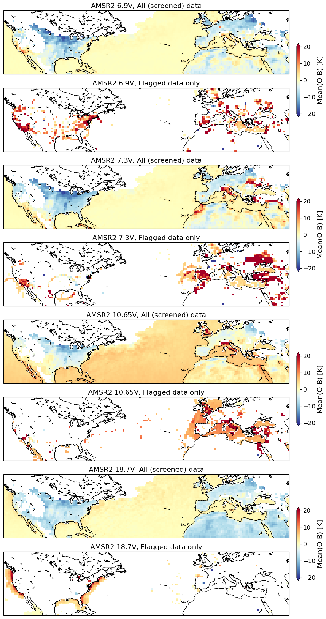
Figure 14 Mean departures from AMSR2 channels 6.9V, 7.3V, 10.65V, and 18.7V comprising data from March 2022. Plots alternate between all observations that passed the screening criteria (top) and RFI-flagged observations only (bottom). At least 1000 observations need to exist in a grid box for it to be plotted, and at least 10 flagged observations for the bottom panels.

Due to atmospheric and surface variability, well-identified RFI will not exclusively manifest as positive departures, but will generally produce positive departures in the aggregate. Strong and/or persistent contamination should thus be red in the figure. The monthly mean departures for all data do indicate some regions for which frequent RFI can be picked out by eye without any filtering: e.g. Morocco and Ukraine at 7.3V or England and Italy at 10.65V. These are clearly regions with persistent contamination. For flagged points only, the expectation is that skillful detection would identify positive departures in the aggregate – lighter red for weak or infrequent true RFI, and dark red for consistently strong RFI. Most of the flagged points do match with positive mean departures, with larger magnitudes typical over land and weaker but more widespread RFI over sea. Some of the main features found by EORFIScan in Fig. 5 – e.g. reflected contamination at 10.65V around Europe and 18.7V around the USA – are verified by the departure analysis. Many smaller features that are either not persistent or not strong enough to be clear in Fig. 5 are visible in Fig. 14, including the Nile Valley at 10.65V, Southern California at 6.9V, Spain at 7.3V, and so on.

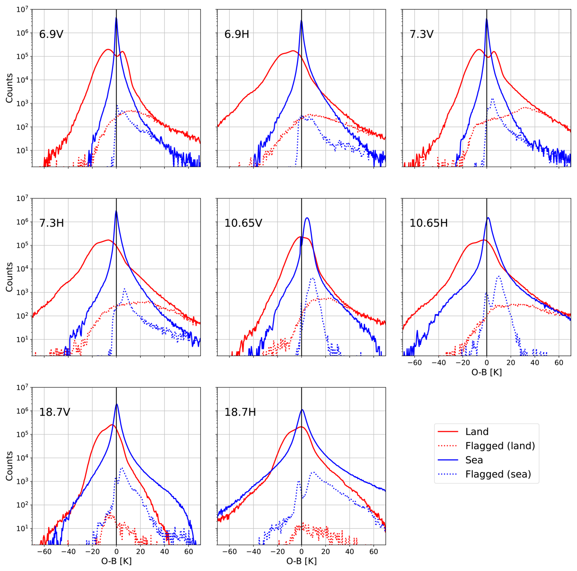
Figure 15 Histograms of departures for screened observations over land (red; > 95 % land fraction) and sea (blue; < 1 % land fraction), comprising data from March 2022. The histograms of all points are given by solid lines, with the flagged histograms given by dotted lines. Region is the same as for the previous figure.

Along the same lines, aggregate departures can be analysed across this region by separating points by land and sea. Figure 15 provides histograms of departures from this region, showing all data and flagged data from land and sea separately. This allows investigation of relative thresholds of detection and viewing the symmetry of the departures. It is clear that EORFIScan flags a large majority of very positive departures at 6.9 and 7.3 GHz over both land and sea, with nearly all departures larger than +30 K flagged as likely contamination at 6.9V, for example. In these cases, it is quite likely that these are indeed RFI, as the departure PDFs have long positive tails. In general, EORFIScan flags very few negative departures, especially over sea, and this indicates a low rate of false positives. It is interesting to note that the histograms are significantly wider for H channels than for V at all frequencies, as might be expected from the larger dynamic range at H. Possibly as a result of this, EORFIScan is more cautious in flagging for H channels. This means that detection thresholds appear larger at H channels, as can be seen in the histogram peaks for flagged data over sea especially. One further feature to note is that EORFIScan thinks that most contamination over sea is fairly weak, with most cases being between about +5 and +20 K departures; this is in contrast to much of the contamination over land, where +20 K signals are common and 7.3 GHz contamination is typically a +25 K signal or more.

5.3 Validation Discussion and Critique

One aspect that is very important for data assimilation is that RFI screening does not remove real, natural signals of clouds and precipitation. This is more of a concern for higher frequency channels due to hydrometeor sensitivity generally increasing with frequency. The challenge for good RFI identification is to retain the natural signals while having a detection threshold that is low enough for the application of interest. Judging the performance of EORFIScan is not quite as easy as simply ensuring that the departure standard deviation decreases globally – if the flagging removes too many points with real geophysical signals, then it is undesirable.

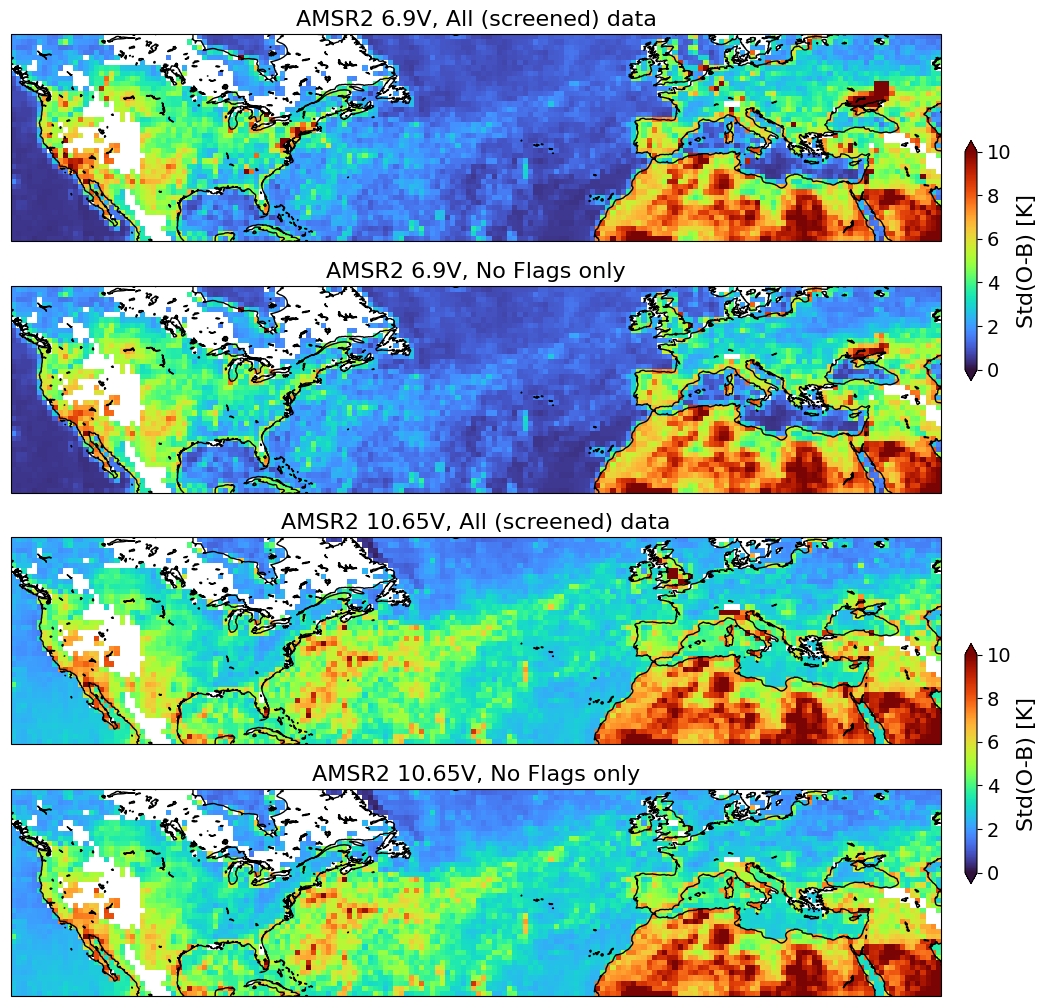
Figure 16 Standard deviation of departures for all screened observations (top) and just observations with no flag (bottom) from AMSR2 channels 6.9V and 10.65V, comprising data from October 2022. At least 1000 (screened) observations need to exist in a grid box for it to be plotted.

With this in mind, Fig. 16 shows the standard deviation of departures before and after flagged data have been removed at 6.9V and 10.65V, now over October 2022 rather than March. Comparing the top and bottom panels, there are regions in which likely contamination appears almost entirely removed by EORFIScan flagging, for example over the UK at 10.65V or the northeast US at 6.9V. Some regions like southeast Ukraine do appear much improved after screening at 6.9V, but significant contamination remains. Outside of the known areas of contamination, the standard deviations of departures appear almost entirely unchanged; examples include the northwestern Atlantic in the Gulf Stream and the Sahara and Arabian deserts, in which large variability is expected and indeed retained by EORFIScan. This indicates that false positives are not significantly dampening the natural variability of departures.

Balancing detection against false positives is difficult to assess for RFI because there is not a truth dataset to compare against, and assessing the detection threshold is similarly challenging because low-level RFI is particularly hard to identify. In our analysis, negative departures represent likely (but not certain) false positives if they are flagged. With this definition of false positives, EORFIScan has a false positive rate of between 0.05 % to 0.2 %, depending on the frequency. Given this low rate of false positives, it could be suggested that the flagging is primarily identifying larger instances of RFI. Going back to the swath-level view of Fig. 13, it does appear that flagging is rare near coastlines, and some points of likely RFI remain in the un-flagged maps of Fig. 16 along coastlines.

This balance is more difficult for H channels where the range of natural variability is larger because of more variable emissivity. The histograms of Fig. 15 suggest that detection limits of EORFIScan are perhaps twice or more what they are at V, though 10.65 GHz departures over sea are an interesting outlier with most flagged departures lying between about +8 to 15 K at both polarizations. It is hard to say anything definitive about the strength of expected contamination because these could conceivably be quite different at V and H at the same frequency band. But if the assumption is that RFI magnitudes are similar across polarizations then the detection skill is stronger at V over both land and sea, especially at C-band.

6 Conclusions

This paper described an assessment of key passive microwave bands exploited for Earth Observation from the 6.4–7.3 GHz band to 174–191 GHz. First the EORFIScan software has been described, which applies multiple RFI detection techniques to EO brightness temperature products. This part includes a description of the RFI detection techniques and the methodology to compute the thresholds. The software has then been used to analyze a year of AMSR2, AMSU-A, MWHS-2, and AMR-C data in order to cover all main EO passive microwave bands beyond the L-band. The methodology has been assessed for AMSR2 and AMSU-A via comparisons with NWP model equivalents, with results presented for the 6–19 GHz bands on AMSR2, where the large majority of corroborated RFI was found. RFI probability maps for 2022 have been computed as the number of detections over the number of observations accounting for all polarizations and orbital passes.

The results have shown heaviest contamination in the 6.4–7.3 GHz band, more moderate contamination at 10.7 and 18.7 GHz bands. The identified areas of systematic contamination have been assessed using all-sky NWP departures, and in most cases are found to correlate strongly with positive departures as would be expected for skilful flagging of RFI. Several new sources are observed in these bands with respect to the literature and corroborated by the NWP-based analysis. The emergence of 6.9 GHz contamination over sea is particularly troubling, as this is a key band for all-weather SST and sea-ice measurements (Scanlon et al., 2025), and will be flown on the upcoming CIMR mission from ESA as well as on the successor instrument to AMSR2, AMSR3. First RFI signatures have been found at 23.8 and 36.5 GHz in AMSR2.

Consideration of RFI detection systems in these bands is strongly advised as part of future mission planning, as the contamination observed already has an impact on users and may be expected to worsen in the upcoming years. At bands from 50 GHz and up, no significant contamination has been detected in the dataset under consideration. However, the constantly evolving threat of RFI in EO bands would benefit greatly from monitoring in real time, especially for bands of consequence for NWP and other operational applications. It is clearly suboptimal to discover new sources of contamination a year or two after those radiances have been ingested into a variety of operational models and retrievals, and thus real-time monitoring would provide significant benefit to a wide community of users.

It is reasonable to expect that high-frequency technology will become more accessible, low-frequency bands will become more crowded, and new services will require greater bandwidths in the near future. As a result, higher frequency bands may start showing contamination and RFI at lower frequency bands could become more widespread than it already is, which will threaten their use for Earth observation. Given that new missions take years from design until the end of their operational lifetime, new EO missions should include RFI detection and mitigation systems to be prepared for the expected worsening of the RFI environment.