Improving imputation of missing PM_2.5 speciation data using PMF-informed source-receptor relationships

Missing values are ubiquitous in atmospheric monitoring due to instrument drift, calibration cycles, operational interruptions, and other random malfunctions. Such gaps can undermine the reliability of subsequent analyses and introduce systematic biases. Conventional imputation methods, such as geometric mean substitution, K-nearest neighbor (KNN), Bayesian principal component analysis (BPCA), and deep learning models often rely primarily on statistical correlations, may require auxiliary inputs, and offer limited physical interpretability. To address this issue, we propose a novel source-receptor-informed Positive Matrix Factorization Reconstruction (PMFr) method that leverages PMF-derived source-receptor relationships, rather than purely statistical interpolation, to impute missing PM_2.5 speciation data without requiring auxiliary data. Benchmarking on a two-month dataset against commonly used imputation techniques, including KNN, BPCA, and a deep learning predictive model, demonstrates that PMFr achieves superior accuracy and robustness across real-world missing scenarios, with a mean coefficient of determination (R²) of 0.81, index of agreement (IoA) of 0.92, and mean absolute percentage error (MAPE) of 22.8 %, reducing MAPE by 25.5 %–29.1 %, particularly for key PM_2.5 species. Further PMF-based validation shows that PMFr better preserves source-profile composition and source-contribution temporal features, indicating that the completed dataset retains more physically meaningful source information and is more suitable for source apportionment. These results highlight PMFr as a robust and physically interpretable approach for reconstructing reliable PM_2.5 speciation data.

1 Introduction

Ambient fine particulate matter (PM_2.5) remains a pressing global environmental challenge due to its well-documented impacts on climate forcing, atmospheric visibility degradation, and adverse health outcomes (Liu and Matsui, 2021; Peng et al., 2023; Hao et al., 2023; Kim et al., 2025b). These effects are governed by the chemically diverse nature of PM_2.5, which comprises inorganic ions, carbonaceous materials, trace metals, and other species. Comprehensive PM_2.5 speciation measurements are therefore fundamental for tracking source contributions, elucidating atmospheric processes, and evaluating their diverse impacts. However, missing data are ubiquitous in both routine monitoring networks and intensive field campaigns due to instrument drift, calibration cycles, operational interruptions, and other random malfunctions (Yu et al., 2017). Such gaps can undermine the reliability of subsequent analyses and introduce systematic biases. Consequently, accurate and robust imputation of missing values is essential, as inappropriate handling of missing data can lead to distorted interpretations and erroneous scientific conclusions.

A wide range of methods have been developed to address missing values in PM_2.5 chemical component datasets, generally falling into listwise deletion, simple substitutions, and advanced statistical models (Alwateer et al., 2024). Basic approaches such as listwise deletion and mean or median substitution, although recommended in the U.S. EPA's guidelines for their simplicity (Norris et al., 2014), often compromise data quality: listwise deletion discards samples containing any missing species and substantially reduces statistical power, whereas median or mean substitution introduces bias that becomes more pronounced as data variability increases (Emmanuel et al., 2021; Polissar et al., 1998; Khan and Hoque, 2020). Linear interpolation is also frequently applied because of its ease of implementation, yet its performance is highly sensitive to the temporal pattern and extent of missingness (Samal et al., 2021; Junninen et al., 2004). To better capture inter-species correlations and nonlinear dependencies, more advanced techniques, including KNN, BPCA, and deep learning models such as deep belief networks (DBN), have been explored and often outperform simpler methods (Lee et al., 2023; Lai and Kuok, 2019; Zaini et al., 2022; Xie, 2017; Shen et al., 2018). Nevertheless, these statistical and machine-learning approaches typically rely on mathematical interpolation, may require auxiliary inputs such as meteorological variables or satellite-derived AOD, and offer limited physical interpretability (van Donkelaar et al., 2019; Lee et al., 2024; Hu et al., 2014; Kim et al., 2024, 2025a). As a result, accurately reconstructing missing PM_2.5 chemical species remains a methodological challenge.

To address these limitations, we develop a physically interpretable imputation method grounded in air pollution source-receptor principles to reconstruct missing PM_2.5 chemical species. Source contributions and profiles are first resolved from pre-existing speciation data using Positive Matrix Factorization (PMF), which decomposes the dataset into a source chemical profile matrix and its corresponding contribution matrix. Under the commonly assumed temporal stability of source chemical compositions, the resolved profiles are then used to reproduce new PM_2.5 speciation datasets containing missing species by multiplying the estimated source-specific PM_2.5 mass by the resolved source profiles, enabling estimation of missing values based on physically meaningful source signatures. This approach ensures that reconstructed concentrations align with both chemical structure and emission characteristics rather than relying solely on mathematical interpolation. To evaluate performance, we generated artificial missing data in complete-speciation datasets; the proposed method was then compared against geometric mean substitution, linear interpolation, K-nearest neighbors (KNN), deep belief networks (DBN), and Bayesian principal component analysis (BPCA). The datasets completed by each imputation method were subsequently used as PMF inputs to assess how different imputation strategies influence downstream source apportionment results. This study highlights the potential of a source-informed strategy for robust and interpretable imputation, as well as for generating completed datasets suitable for subsequent source apportionment and chemical-constrained health and climate impact analyses.

2 Material and Methods

2.1 Sample Collection and Data Processing

Hourly PM_2.5 speciation data were collected on the rooftop of the Nanjing Environmental Protection Building (NEPB, 118.75° E, 32.06° N). Water-soluble inorganic ions including NH${}_{\mathrm{4}}^{+}$, SO${}_{\mathrm{4}}^{\mathrm{2}-}$, NO${}_{\mathrm{3}}^{-}$, Cl⁻, Ca²⁺, Mg²⁺, K⁺, and Na⁺ were determined by MARGA (ADI 2080; Applikon Analytical B.V., the Netherlands). Hourly OC and EC concentrations were measured using a semi-continuous OC/EC analyzer (RT-4, Sunset laboratory Inc., USA) with the NIOSH method 5040 (Birch, 2002). An Xact 625 ambient metals monitor (Cooper Environmental, United States) was configured to quantify twenty-three elements (K, Fe, Zn, Ca, Si, Mn, Pb, Cu, Ti, As, V, Ba, Cr, Se, Ag, Cd, Ni, Au, Co, Sn, Sb, Tl, and Hg). Detailed information on the monitoring site, instrument setup and maintenance, and chemical analysis were reported by studies (Yu et al., 2019, 2020; Xie et al., 2022).

The dataset used in this study comprises inorganic ions (NH${}_{\mathrm{4}}^{+}$, SO${}_{\mathrm{4}}^{\mathrm{2}-}$, and NO${}_{\mathrm{3}}^{-}$), trace elements (K, Fe, Zn, Ca, Si, Mn, Pb, Cu, Ti, As, V, Ba, Cr, and Se), and carbonaceous materials (OC and EC), which were measured from 1 October 2017, 01:00 am local time (LT, GMT+8) to 30 November 2017, 11:00 pm LT. The summary for the missing of raw data can be seen in Table S1 in the Supplement.

2.2 Missing Data Generation

Four factors are considered to affect the performance of imputation methods: the missing-data generation mechanism, the proportion of missing data, the gap pattern of missing data (Junger and Ponce de Leon, 2015), and whether multiple species are missing simultaneously (MCMS) or independently (MCMI). Specifically, MCMS refers to the simultaneous absence of multiple species at a single timestamp, while MCMI denotes missing values occurring independently at distinct timestamps.

The mechanisms of missing values are typically classified into three categories (Little and Rubin, 2019): (i) missing completely at random (MCAR), where missing values are generated independently, namely independent of both observed and unobserved values. (ii) missing at random (MAR), where missingness is related to observed data, and (iii) missing not at random (MNAR), where missing values are related to unobserved data such as values below the detection limit (BDL). Analysis of the NEPB dataset shows no systematic association between missing occurrences and pollutant concentration levels or temporal patterns, indicating that the missingness does not follow the MNAR mechanism (García-Laencina et al., 2010). Consequently, missing data were generated randomly to ensure that the artificial missingness remained independent of pollutant concentrations.

The proportion of missing data is a critical factor affecting imputation performance. In this study, missingness rates of 10 %, 15 %, and 20 % were imposed, matching the observed range of 10 %–20 % in the monitored dataset.

Gap pattern refers to the proportion of different gap lengths within the total missing data. Based on the summary of the missing data, the physical meaning and prior research (Plaia and Bondì, 2006; Betancourt et al., 2023; Jing et al., 2022; Richardson and Hollinger, 2007), gap lengths (l) were categorized into three types: (i) short gaps, with l from 1 to 6; (ii) medium gaps, with lengths greater than 6 but less than 23; and (iii) large gaps, l ranging from 23 to 115 consecutive values (1 to 5 d), which represents the longest gap observed in the raw dataset (Table S2).

Table 1 Description of different missing scenarios considered in this study.

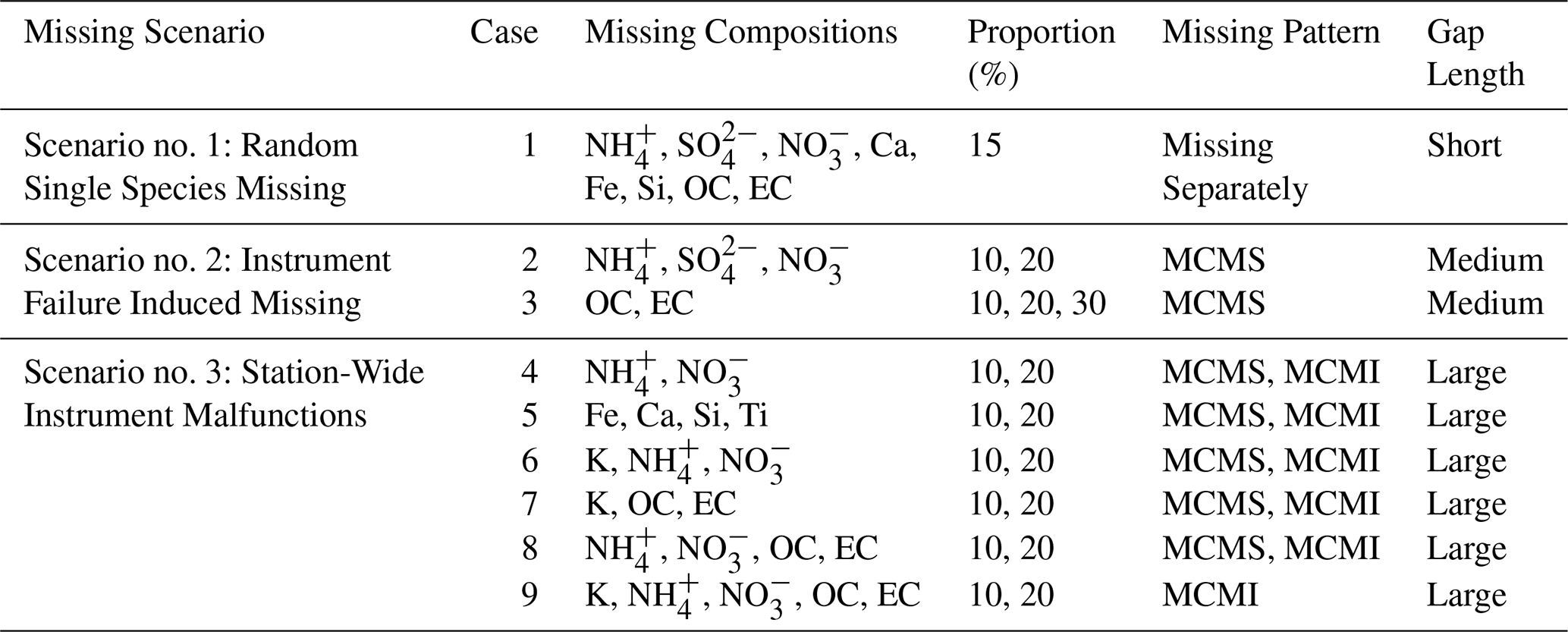
In summary, missing data were generated according to the scenarios listed in Table 1. These scenarios include: (i) random single-species missing that create short gaps in individual species (Case 1); (ii) instrument-failure-induced missing that produce medium gaps across all species measured by a given instrument, affecting ionic (Case 2) and carbonaceous (Case 3) monitors; and (iii) station-wide instrument malfunctions that result in large gaps spanning multiple species. These scenarios include malfunction of the ionic monitoring instrument (Case 4) and elemental monitoring instrument (Case 5), concurrent malfunction of two instruments (Cases 6–8), and malfunction of all monitoring instruments (Case 9). Potassium (K) was treated as missing in multi-instrument malfunction scenarios (Cases 6, 7 and 9) due to its strong correlations with both ionic and carbonaceous species (Fig. S1). The performance of the imputation methods was evaluated using the coefficient of determination (R²), the mean absolute percentage error (MAPE), and the index of agreement (IoA) (Sect. S1.2).

2.3 Source-Receptor Informed Positive Matrix Factorization Reconstruction (PMFr) and Validation

A source-tracer for imputation, hereafter referred to as a tracer, is defined as a key species that distinguishes a specific factor (source) from others and reflects how that factor (source) influences the receptor over time. Co-tracers refer to co-varying tracers of the same factor, collectively characterizing the temporal behavior of the corresponding source. As illustrated in Fig. 1, PMF is first applied to resolve factor profiles and their contributions, providing source-receptor relationships constrained by expert knowledge, given that pollution sources imprint distinct temporal patterns on the receptor site. Details of the usage of PMF for SA can be found in the literature, and the uncertainty settings are provided in Sect. S1.3 (Hopke, 2016; Paatero, 1999; Paatero and Hopke, 2003). Based on the SA results with selected source profiles, species requiring imputation are classified as tracers or non-tracers through a knowledge-driven step (Bi et al., 2019). When imputing tracers, the availability of co-tracers should be checked at each timestamp before reconstruction, because the source contribution vector (g) needs to be constrained by source-specific tracer information. If all tracers associated with a specific factor are simultaneously missing, the corresponding g vector is less directly constrained by observed species; in such cases, these missing tracer values are first imputed using another imputation method, with KNN recommended for its simplicity, efficiency, and ability to provide a reasonable estimate of temporal variation. The corresponding uncertainty is set to 10 % of the imputed concentration. For missing tracers with available co-tracers, as well as for non-tracers, missing values are replaced by the geometric mean. The uncertainty calculation is further discussed in Sect. S1.4. The pre-imputed dataset and its associated uncertainty matrix are then fed into the PMF analysis for reconstruction. The PMF run decomposes the dataset into factor profiles (F) and source contributions (G), and data reconstruction is achieved by multiplying the G and F matrices. Rather than relying directly on covariance in the high-dimensional chemical dataset, PMFr reconstructs missing values within this low-entropy source structure represented by PMF-resolved source profiles and temporal contributions.

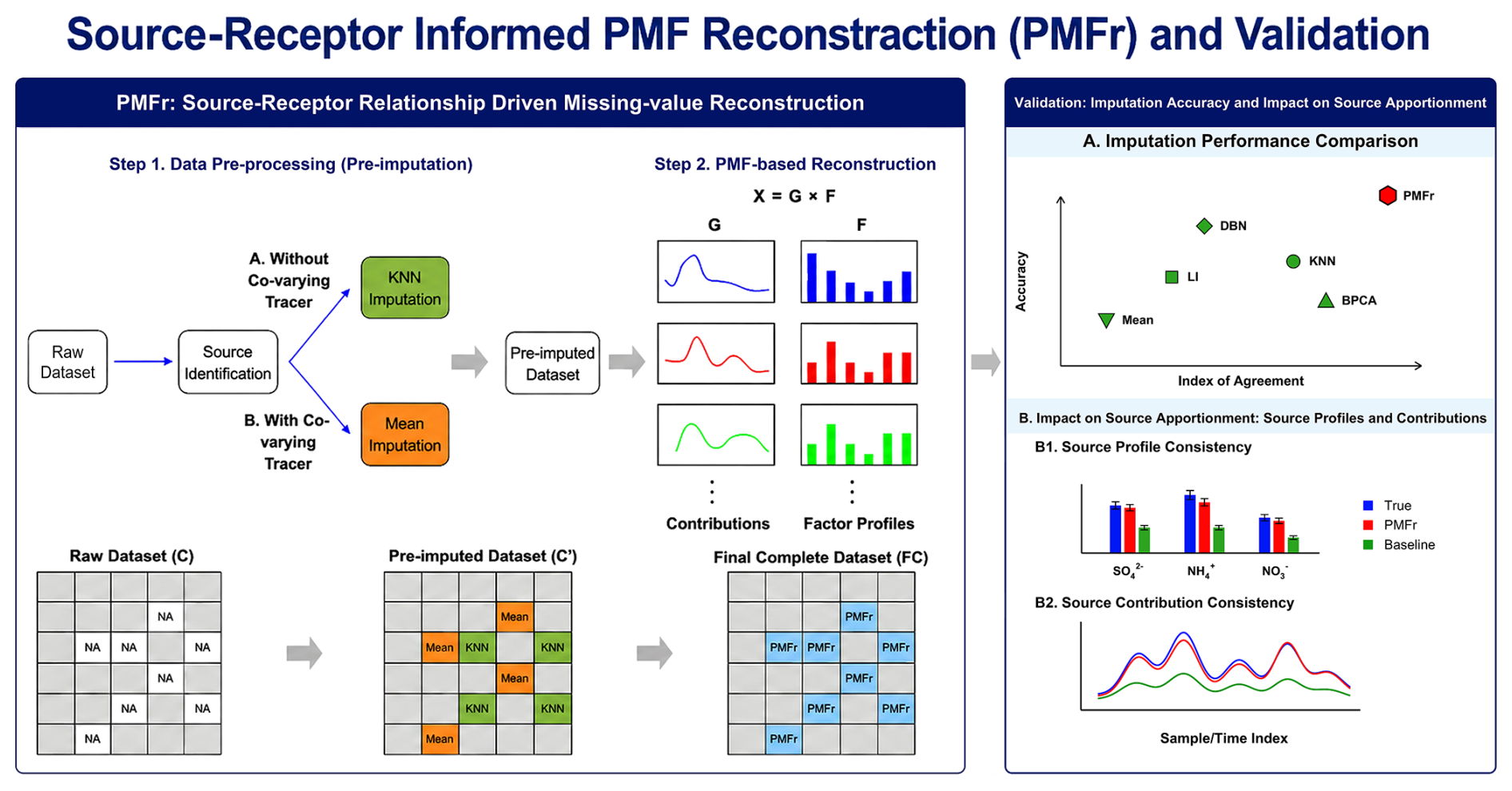
Figure 1 Flow chart of source-receptor informed Positive Matrix Factorization Reconstruction (PMFr) and validation.

The performance of PMFr was evaluated using two complementary validation endpoints: direct reconstruction accuracy and physical source-feature preservation. The reconstructed concentrations were directly compared with observed values and benchmarked against baseline methods, including LI, KNN, DBN, BPCA, and geometric mean imputation (Mean), using R², IoA, and MAPE. The U.S. EPA PMF 5.0 User Guide recommends handling missing values by replacing them with the species median and assigning a high uncertainty to downweight these substituted values. Here, missing values were replaced by the species-specific geometric mean, following the same constant-substitution and downweighting principle. Because the geometric mean is also a robust central value for skewed data and was adopted in the previous PMF analysis using the same hourly PM_2.5 speciation dataset (Xie et al., 2022), it was used here as a representative conventional PMF missing-value treatment for comparison with PMFr. Physical source-feature preservation was further assessed by comparing the PMF-resolved source profiles and corresponding source contributions obtained from different imputed datasets with those derived from the original complete dataset.

3 Results and Discussion

3.1 Source-receptor relationship resolved by PMF

PMF solutions were explored from four to nine factors using datasets containing 10 % missing values. The best-fitting solution was selected by the model performance, including the interpretability of the factor profiles, which is essential for determining the optimal factor number and imputation, and the distributions of scaled residuals (Reff et al., 2007; Brown et al., 2015; Dai et al., 2020, 2021) (Figs. S2 and S3). Bootstrapping (BS), displacement (DISP), and combined BS-DISP analyses were also performed for these solutions(Paatero et al., 2014; Liu et al., 2017; Wang et al., 2018). Four-to-six factor solutions were statistically insufficient to fully explain the variance in the input data matrix. When the factor number increased from six to seven, the $Q/Q_{\exp }$ ratio experienced a decline of 11.2 %. This drop indicates that the 6-factor model leaves a substantial amount of residual variance unexplained. Specifically, the 5-factor solution improperly lumped on-road traffic emissions with metal smelting (Fig. S5). In the 6-factor solution, sulfate and nitrate were mixed together as a single identified secondary inorganic aerosol factor (Fig. S6). Eight and nine factor solutions demonstrated statistical over-resolution with diminishing returns. As the factor number increased from seven to eight, the $Q/Q_{\exp }$ ratio dropped less dramatically (8.5 %) compared to the previous step. Furthermore, the 8-factor solution exhibited a high unmapped rate during the BS analysis, highlighting statistical instability. From a physical perspective, these higher-factor solutions over-resolved the data into physically meaningless profiles. For instance, the 8-factor solution isolated a Cu-high loading factor that lacks a clear chemical profile (Fig. S7), while the 9-factor solution further fragmented the coal combustion into two unidentifiable sources (Fig. S8). For the 7-factor solution, the model predicted concentrations of tracers such as Ca, V, ${\mathrm{NH}}_{\mathrm{4}}^{+}$, and ${\mathrm{NO}}_{\mathrm{3}}^{-}$ correlated with the observed values with coefficients of determination (R²) of 0.92, 0.91, 0.98, and 0.88, respectively (Table S4). The high R² values of bulk species indicate that the 7-factor model fits well for the data. For tracers like Si, Mn, Se, and Cu, the scaled residuals follow a normal distribution with a mean of 0 and a variance of 1. For bulk species like ${\mathrm{NH}}_{\mathrm{4}}^{+}$, ${\mathrm{NO}}_{\mathrm{3}}^{-}$, and ${\mathrm{SO}}_{\mathrm{4}}^{\mathrm{2}-}$, the scaled residuals exhibit a small-tailed distribution, with the highest frequency concentrated near 0 and ranging from −2 to 2. Additionally, the scaled residuals of the bulk species OC and EC follow a normal distribution with a mean of 0 and a variance of 1. The distribution of scaled residuals demonstrates the validity of our solution. Physically, the 7-factor solution successfully decouples all distinct emission sources without redundant splitting. The first factor was interpreted as Coal Combustion (CC), characterized by high explained variances of Pb, As, and Se (Cheng et al., 2015) and higher daytime concentrations (Fig. S10a) (Li et al., 2020). These species have relatively low DISP intervals. The Heavy Oil Combustion (HOC) was characterized by V and Ni, which are tracers of HOC (Becagli et al., 2012). The presence of HOC is consistent with the fact that Nanjing is the biggest container port on the Yangtze River. The Metal Smelting (MS) factor was identified with high Cr, Fe, Mn, Zn and Ni explained variances. Cr, Mn, Zn and Fe are typically emitted from iron and steel production (Chang et al., 2018; Pekney et al., 2006), and they exhibit relatively low DISP intervals. Cu and Ba, along with high loadings of OC and EC, serve as tracers for On-road Traffic (OT), reflecting vehicle exhaust and non-exhaust emissions such as brake and tire wear (McKenzie et al., 2009; Becagli et al., 2012). OT is also identified by high loadings of OC and EC, with the increase of concentration during the rush hour (Fig. S10d). The Crustal Dust (CD) factor is composed of crustal elements Ca, Si, Ba, Fe and Ti (Wang et al., 2018). The remaining two factors are Secondary Sulfate (SS) and Secondary Nitrate (SN), whose tracers are sulfate for SS, and ammonium and nitrate for SN, respectively. SS and SN exhibit enhanced formation around midday and nighttime, respectively (Fig. S10f and g). The following reconstruction process will be based on the 7-factor solution.

3.2 Comparison of Imputation Methods under Different Missing Scenarios

3.2.1 Overall Performance under All Missing Scenarios

As shown in Fig. S30, the PMFr method achieves the overall R² of 0.81 and MAPE of 22.8 % under the three evaluated missing scenarios. In comparison, DBN results in an R² of 0.73 and a MAPE of 32.2 %, BPCA yields an R² of 0.72 and a MAPE of 30.6 %, and KNN achieves an R² of 0.72 and a MAPE of 31.2 %. For simple baseline methods, LI produces an R² of 0.35 and a high MAPE of 61.7 %, while the geometric mean imputation method (Mean) results in a higher MAPE of 66.75 %. Given that mean imputation produces a constant value without temporal variation and consistently fails to provide effective reconstruction across individual scenarios (Figs. S11–S29), its performance is solely quantified by MAPE here and is excluded from further detailed comparisons in subsequent sections. Furthermore, the Taylor diagram (Fig. S31) illustrates that the PMFr reconstructed data yield a normalized standard deviation (σ) of 0.93, closely matching the observational variance (σ=1.0), suggesting its capability to capture the amplitude of data variations.

3.2.2 Scenario no. 1: Random Single Species Missing

As shown in Fig. 2, PMFr achieves the highest mean IoA (0.96) and lowest mean MAPE (16.88 %), both with low standard deviations. Both PMFr and DBN attain the highest mean R² of 0.86, with DBN exhibiting a lower standard deviation.

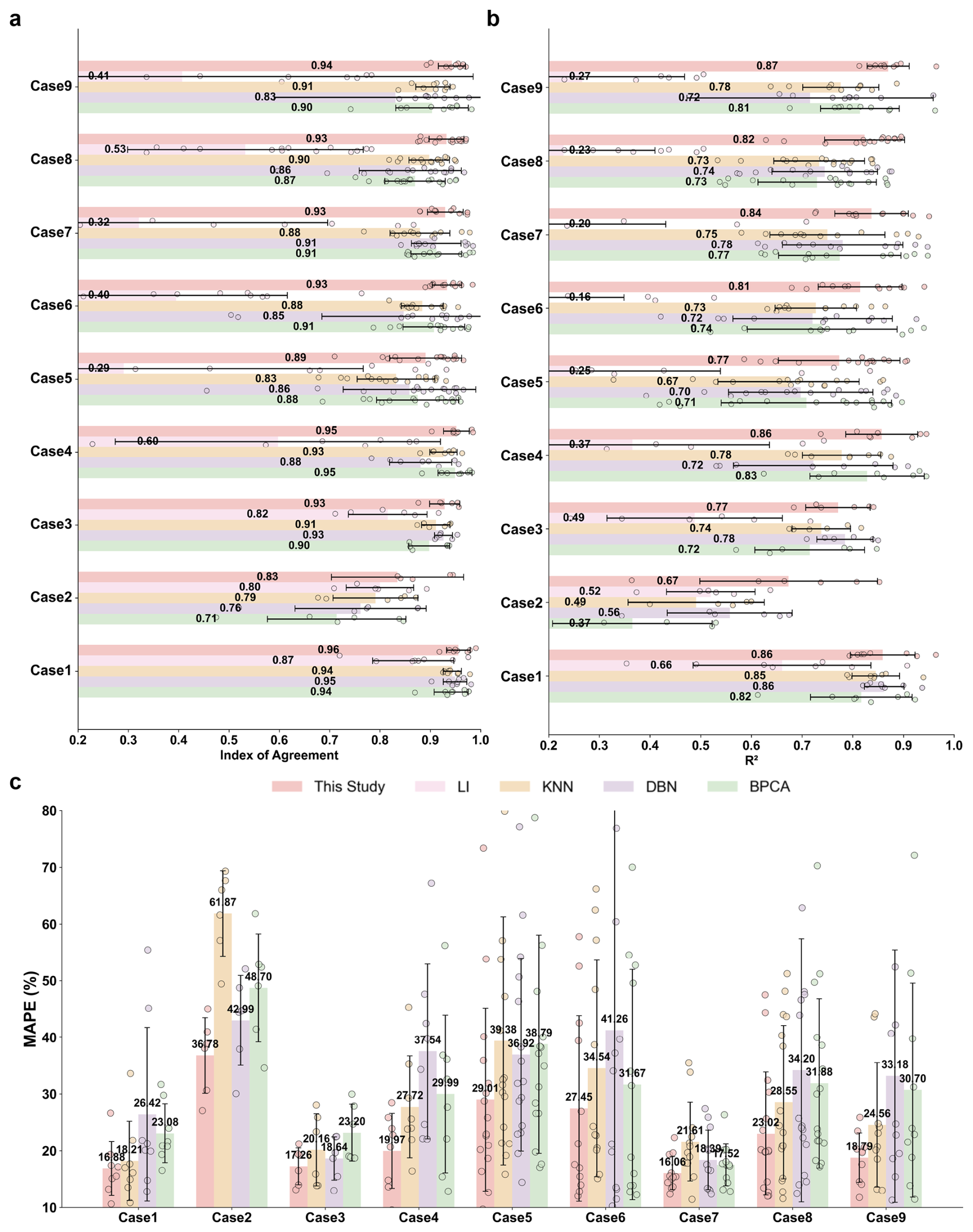
Figure 2 Performance of five imputation methods across nine Cases. Asymmetric error bars indicate the standard deviation. Points show the performance for individual species. (a) R², (b) IoA, and (c) MAPE, where LI method is excluded due to poor performance under system failure conditions.

For inorganic ions, PMFr performs best when imputing ${\mathrm{NH}}_{\mathrm{4}}^{+}$ and ${\mathrm{NO}}_{\mathrm{3}}^{-}$ with R² values of 0.96 and 0.91, respectively. PMFr shows the highest agreement with the observed values when imputing ${\mathrm{NH}}_{\mathrm{4}}^{+}$ and ${\mathrm{NO}}_{\mathrm{3}}^{-}$, especially for both low and high concentrations (Figs. S11 and S12). The performance of PMFr declines when imputing ${\mathrm{SO}}_{\mathrm{4}}^{\mathrm{2}-}$, with R² = 0.79, IoA = 0.92 and MAPE = 15.09 %. Nevertheless, PMFr still outperforms LI, KNN, and BPCA. PMFr achieves higher R² and IoA (0.83 and 0.96, respectively), but it attains a lower MAPE (15.09 %) compared to DBN (19.81 %). As shown in Fig. S12, values imputed by PMFr show better agreement with true observations when the missing data correspond to low ${\mathrm{SO}}_{\mathrm{4}}^{\mathrm{2}-}$ concentrations. All methods except LI struggle to accurately impute high ${\mathrm{SO}}_{\mathrm{4}}^{\mathrm{2}-}$ concentrations. The absence of other cations like Na⁺ and Mg²⁺ may impact the imputation efficiency when the missing ${\mathrm{SO}}_{\mathrm{4}}^{\mathrm{2}-}$ concentrations are high. This difference is likely because the formation of NH₄NO₃ typically dominates the nitrate fraction, while (NH₄)₂SO₄ accounts for only a portion of the total sulfate.

For elements, PMFr performs well, with R² values of 0.82–0.93, IoA values of 0.95–0.98, and MAPE of 13.21 %–17.17 %, all accompanied by low standard deviations. Compared with PMFr, DBN performs better when imputing Fe, yielding higher R² and IoA, but also a higher MAPE. Conversely, PMFr shows better performance when imputing Ca, particularly for high concentration values (Fig. S14). The proposed method underestimates Fe, whereas DBN shows better consistency for missing observations that correspond to high Fe concentrations. Nevertheless, all methods fail to accurately reconstruct those high Fe concentrations (Fig. S16). LI performs better when imputing elements than ions, indicating that element concentrations fluctuate more steadily.

For carbonaceous materials, PMFr attains the highest IoA (0.94) for OC and the second-highest IoA (0.95) for EC, with low MAPE values of 17.42 % and 15.53 %, respectively. KNN achieves the highest R² (0.86 for OC and 0.87 for EC), although with lower IoA values compared to PMFr. DBN performs worse for OC, especially for low concentrations (Fig. S17). Although LI performs reasonably well for OC, it exhibits weak correlations with the true observations for EC, a trend also observed when imputing ${\mathrm{NO}}_{\mathrm{3}}^{-}$ and ${\mathrm{SO}}_{\mathrm{4}}^{\mathrm{2}-}$, as its performance is easily affected by the distribution pattern of missing data (Junninen et al., 2004). EC is primarily emitted from motor vehicles, whereas OC encompasses both directly emitted primary organic carbon (POC) and secondary organic carbon (SOC) formed through atmospheric processes. The behavior of POC is consistent with partial origins from vehicular emissions, while the variations of SOC are likely associated with secondary sources such as SS and SN (Liao et al., 2023). The proposed method effectively captures SOC by utilizing reasonable factor profiles, whereas other imputation methods fail to reveal the formation of SOC due to limited data. Therefore, PMFr is recommended for imputing missing components caused by random missingness.

3.2.3 Scenario no. 2: Instrument Failure Induced Missing

As shown in Fig. 2, PMFr achieves the highest mean R² (0.67) and IoA (0.83), and the lowest mean MAPE (36.78 %) in Case 2. Although the R² error bar is relatively broad, indicating species-dependent variability in correlation performance, the smaller MAPE error bar suggests that PMFr maintains more stable magnitude accuracy across species. The R², IoA, and MAPE of PMFr range from 0.54–0.81, 0.59–0.95, and 27.09 %–52.01 %. Performance declines for ${\mathrm{SO}}_{\mathrm{4}}^{\mathrm{2}-}$, with IoA values of 0.58 and 0.64 for 10 % and 20 % missingness, respectively. PMFr yields lower MAPE (34.09 % and 52.01 %) when the missing percentages are 10 % and 20 %, respectively. When imputing ${\mathrm{NH}}_{\mathrm{4}}^{+}$ and ${\mathrm{NO}}_{\mathrm{3}}^{-}$, PMFr shows the best agreement with true observed values among all methods, particularly for both low and high concentrations (Figs. S18–S21), owing to the constructed source-receptor relationships, which effectively address the difficulties that machine-learning methods face in capturing extreme values.

In Case 3, the proposed method achieves the highest mean IoA (0.93) and the lowest mean MAPE (17.26 %), both with low standard deviations. Although performance declines relative to Case 1, PMFr remains comparable to DBN, which leverages inter-variable correlations for imputation. The decline is likely attributable to the absence of key tracers, consistent with the tracer-dependent variability observed at the NEPB site – where the strong OC-EC correlation may reflect their common origin in motor-vehicle emissions (Yu et al., 2020). The performance of PMFr may be impacted because PMF tends to overestimate the loading of OC and EC in the OT factor, thereby obscuring their contributions from other sources. Nevertheless, this highlights the interdependence between OC and EC, and the greater decline observed in KNN and BPCA compared with the proposed method.

3.2.4 Scenario no. 3: Station-Wide Instrument Malfunctions

As illustrated in Fig. 2, PMFr achieves the highest mean R², IoA, and the lowest mean MAPE with low standard deviations in Case 4 (0.86 %, 0.95 %, and 19.97 %, respectively) and Case 5 (0.77 %, 0.89 %, and 29.01 %, respectively). In Case 4, PMFr captures the temporal variability of the imputed species more effectively, yielding higher R² and IoA values, particularly for both low and high concentrations of ${\mathrm{NH}}_{\mathrm{4}}^{+}$ and ${\mathrm{NO}}_{\mathrm{3}}^{-}$, indicating the stability of SN even under extreme missing cases. In Case 5, the imputation results show that all elemental species are well reconstructed, with Ti being the only exception. For Ti, PMFr demonstrates the highest accuracy, achieving IoA values between 0.82 and 0.95 and outperforming other methods, especially at low concentration levels (Figs. S26–S29). This improvement is likely associated with the predominant emission of Ti from dust sources, enabling PMFr to estimate missing values by leveraging the characteristic Ti-Ca-Si ratios in source profiles once the CD factor is identified (Wang et al., 2018).

PMFr consistently achieves the highest mean R² (0.81–0.84), IoA (0.93), and the lowest MAPE (16.06 %–27.45 %) under Cases 6–8, all accompanied by low standard deviations. Compared with Case 4, the performance of KNN and BPCA declines in Cases 6 and 8. For KNN, IoA falls from 0.93 to 0.88 (Case 6) and 0.89 (Case 8); for BPCA, IoA declines from 0.95 to 0.89 (Case 6) and 0.90 (Case 8), with both methods showing increased standard deviations. These results indicate that KNN and BPCA become unstable when additional species correlated with ${\mathrm{NH}}_{\mathrm{4}}^{+}$ and ${\mathrm{NO}}_{\mathrm{3}}^{-}$ are missing, with the degradation being substantial in Case 6. In contrast, PMFr remains stable with low standard deviations because ${\mathrm{NH}}_{\mathrm{4}}^{+}$ and ${\mathrm{NO}}_{\mathrm{3}}^{-}$ are estimated from source-receptor relationships – specifically the SN profile – rather than from correlations with species such as K, which are estimated via the CC and CD profiles. In Case 9, PMFr achieves the highest mean R², IoA, and the lowest MAPE (0.87 %, 0.94 %, and 18.79 %, respectively). The strong performance of PMFr, KNN, and BPCA in this MCMI setting is attributable to the abundant co-occurring information, even as the number of missing species increases.

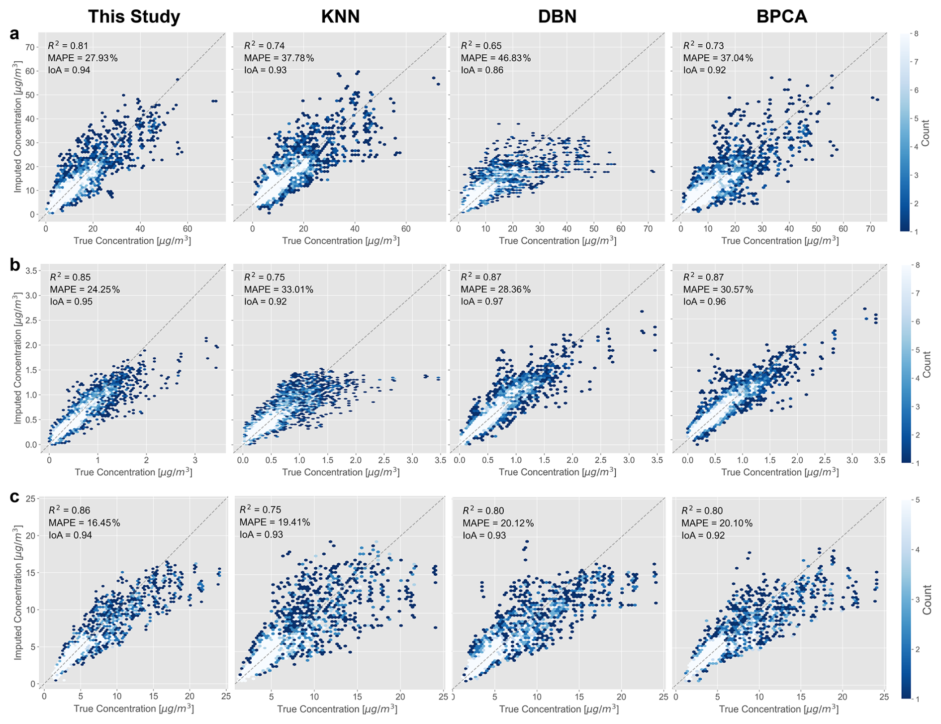
Figure 3 Comparison of observed and imputed values derived from different imputation methods under Scenarios no. 3 (Cases 4–9) stratified by chemical species: (a) Inorganic ions; (b) Trace elements; and (c) Carbonaceous materials.

As shown in Fig. 3a and c, PMFr achieves the lowest MAPE (16.45 % and 27.93 %) and the highest R² (0.81 and 0.86) and IoA (both 0.94) when imputing ionic and carbonaceous species. The performance of DBN declines for ionic species, which may be attributed to insufficient valid training samples and variables caused by long missing gaps and an increasing number of missing species (Liu et al., 2022) (Figs. S22–S25). Furthermore, ${\mathrm{NH}}_{\mathrm{4}}^{+}$ and ${\mathrm{NO}}_{\mathrm{3}}^{-}$ are strongly correlated, a pattern consistent with the predominance of NH₄NO₃ during the fall at the NEPB site (Yu et al., 2020). The absence of either species therefore degrades the performance of machine learning methods, whereas PMFr can reconstruct the ${\mathrm{NH}}_{\mathrm{4}}^{+}$–${\mathrm{NO}}_{\mathrm{3}}^{-}$ relationship using the existing source profiles. When imputing OC and EC, PMFr performs best at low concentration ranges (0–10 µg m⁻³), likely due to their relatively stable emission patterns. The limitations of machine-learning methods for imputing ionic and carbonaceous species have also been reported by Lee et al. (2023), particularly when the number of missing species increases. PMFr achieves the lowest MAPE (24.25 %) for elemental species while still maintaining a high R² (0.85) and IoA (0.95), remaining comparable to DBN, which attains the highest R² (0.87) and IoA (0.97). Machine-learning methods can effectively capture correlations between a target element and co-varying elements (Li et al., 2023), and elemental species are generally emitted directly without undergoing chemical reactions (Choi et al., 2022), which contributes to the strong performance of DBN when imputing elemental species.

3.3 Assessing the Impact of Imputation on PMF Source Apportionment

Results showed that the numerical advantage of PMFr over baseline methods narrowed mainly under two challenging conditions: instrument-failure-type missingness and missingness of specific species such as ${\mathrm{SO}}_{\mathrm{4}}^{\mathrm{2}-}$ and crustal elements such as Fe. Accordingly, two representative cases were selected for downstream PMF evaluation: ${\mathrm{SO}}_{\mathrm{4}}^{\mathrm{2}-}$ missingness in Case 2 at a 10 % missing rate and high-concentration Fe missingness in Case 5 at a 20 % missing rate. The SS and CD factors were used to assess whether these imputation differences propagated into PMF-resolved source profiles and source contributions. For the SS factor (Fig. S32), the ${\mathrm{SO}}_{\mathrm{4}}^{\mathrm{2}-}$ $/$ ${\mathrm{NH}}_{\mathrm{4}}^{+}$ mass ratio derived from the PMFr-completed dataset was 3.39 (${\mathrm{NH}}_{\mathrm{4}}^{+}$ associated with NH₄NO₃ removed), close to that from the complete observed dataset (3.44). BPCA also produced a comparable ratio of 3.33, whereas LI (3.93), KNN (2.91), DBN (2.55), and Mean (3.83) showed larger deviations. This indicates that PMFr better preserved the ${\mathrm{SO}}_{\mathrm{4}}^{\mathrm{2}-}$–${\mathrm{NH}}_{\mathrm{4}}^{+}$ relationship in the SS profile, which is critical for maintaining the chemical interpretability of the SS factor. For the CD factor (Fig. S33), PMFr also reproduced the crustal elemental ratios consistently. The Fe $/$ Ca and Ca $/$ Si ratios from the complete observed dataset were 0.93 and 1.64, respectively, while PMFr yielded corresponding values of 0.95 and 1.62. In contrast, larger deviations were observed for several baseline methods, such as DBN for Fe $/$ Ca (1.21) and BPCA or LI for Ca $/$ Si (1.43 and 1.44, respectively). These results suggest that inappropriate imputation can alter the resolved source-profile composition, whereas PMFr maintains the physical consistency of source profiles.

For the SS factor contributions, PMFr achieved the highest Pearson's correlation coefficient (r) of 0.943, followed by KNN (0.914), BPCA (0.913), LI (0.900), Mean (0.802), and DBN (0.743). For the CD factor contributions, PMFr also showed the highest temporal agreement, with an r of 0.954, followed by Mean (0.948), KNN (0.926), BPCA (0.925), LI (0.796), and DBN (0.706). These results indicate that competitive concentration-level imputation does not necessarily guarantee equivalent preservation of PMF-resolved source-contribution patterns. As shown in Fig. S34a, b, the PMFr-derived SS contribution closely reproduced the diurnal pattern from the original complete dataset, particularly during daytime periods when secondary sulfate formation is expected to be enhanced. Similarly, PMFr captured the diurnal variation of CD more consistently than baseline methods, especially around the daytime peak likely associated with dust resuspension and other daytime dust-related activities. The selected time-series episodes showed the same behavior (Fig. S35a, b). For Case 2 at a 20 % missing rate, PMFr achieved the highest r of 0.985 for SS, compared with BPCA (0.981), KNN (0.980), DBN (0.954), LI (0.936), and Mean (0.705). For the high-Fe missing case, PMFr also showed the highest agreement for CD, with an r of 0.951, followed by Mean (0.928), BPCA (0.888), KNN (0.881), DBN (0.713), and LI (0.683). Therefore, the advantage of PMFr is not limited to pointwise concentration accuracy; it also better preserves the chemical and temporal source structures needed for physically interpretable PMF source apportionment. These results indicate that inaccurate imputation may propagate into PMF analysis and introduce source-apportionment biases, potentially making the imputed dataset less reliable than one processed using conventional PMF missing-value treatments (Kim et al., 2024).

3.4 Applicability and Limitations of PMFr

PMFr is applicable when the chemical profile of each source factor can be constrained by at least one representative tracer, ensuring that the completed remains suitable subsequent source apportionment analysis. One limitation of PMFr is related to missing patterns in which source-related constraints become insufficient. As shown in Table S7, the performance of PMFr declines when the missing pattern shifts from MCMI to MCMS. For ${\mathrm{NH}}_{\mathrm{4}}^{+}$ at a 10 % missing rate, the MAPE increases from 9.57 % under MCMI to 20.67 % under MCMS, and the IoA decreases from 0.98 to 0.95. For ${\mathrm{NO}}_{\mathrm{3}}^{-}$ at a 10 % missing rate, the MAPE increases from 14.82 % under MCMI to 23.92 % under MCMS. At a 20 % missing rate, the MAPE increases from 13.63 % to 25.87 % for ${\mathrm{NH}}_{\mathrm{4}}^{+}$, and from 22.81 % to 28.46 % for ${\mathrm{NO}}_{\mathrm{3}}^{-}$. As shown in Table S6, when OC and EC are simultaneously missing, the performance of PMFr becomes comparable to that of baseline methods. For instance, at a 10 % missing rate, the R² values for OC are 0.73 for PMFr, 0.74 for DBN, 0.68 for KNN, and 0.66 for BPCA. For EC, R² values are 0.84 for PMFr, 0.85 for BPCA, 0.80 for DBN, and 0.79 for KNN. Fundamentally, PMFr assumes that the source contribution vector (g) can be sufficiently constrained by observed species, which requires at least one key tracer for each factor. The key tracers used for imputation and source identification are shown in Table S13. If all key tracers for a specific source are simultaneously missing, the corresponding source contribution vector (g) is less directly constrained by observed species and should be interpreted with caution. Nevertheless, sensitivity analysis indicates that PMFr can still outperform baseline methods when the pre-imputation step provides a reasonable estimate of the general temporal variation of the missing species (Sect. S1.5 and Table S14). The numerical advantage of PMFr is less substantial for certain species such as ${\mathrm{SO}}_{\mathrm{4}}^{\mathrm{2}-}$ and crustal elements. For crustal elements, baseline methods can become competitive because these species are primarily emitted directly and usually exhibit relatively stable inter-variable correlations. As shown in Table S5, when imputing Ca, Si, and Fe at a 15 % missing rate, several statistical or machine-learning methods perform comparably to PMFr. For Ca, the R² values are 0.93 for PMFr, 0.91 for BPCA, and 0.90 for DBN. For Si, PMFr achieves an R² of 0.82, which is matched by DBN and closely followed by KNN (0.79). For Fe, the R² values are 0.83 for PMFr, 0.86 for DBN, 0.84 for KNN, and 0.84 for BPCA, with DBN and KNN achieving slightly higher IoA values than PMFr. This reduced separation suggests that statistical or machine-learning methods can capture stable co-variation patterns among some primary species, thereby reducing the relative advantage of the source-constrained PMFr method for these specific cases. However, comparable concentration-level performance does not necessarily imply that baseline methods are equally reliable for source apportionment. The PMF evaluation results showed that PMFr better preserved source-profile composition and source-contribution temporal patterns, even in representative cases where direct imputation metrics became comparable among methods.

Another limitation of the PMFr lies in the assumption of relatively stable source profiles. In PMFr, source profiles are assumed to remain stable so that the source-receptor relationships resolved by PMF can be used to guide missing-value reconstruction. This assumption is generally more reasonable for short-term datasets, but it may become weaker for long-term datasets, especially those spanning multiple years, during which emission patterns and atmospheric processes can change substantially. Therefore, source-profile stability should be evaluated before applying PMFr in extended applications. Moving-window PMF approaches provide a promising way to examine source-profile stability in long-term applications by resolving time-dependent factor profiles within short moving windows and screening accepted PMF solutions using source-specific criteria, such as factor-tracer correlations, diurnal patterns, and PMF diagnostics and non-modeled time points (Song et al., 2021; Canonaco et al., 2021). Improvements of PMFr could incorporate time-dependent source profiles to address this limitation and better support reconstruction under changing atmospheric conditions.

4 Conclusion

We developed a physically interpretable imputation method (PMFr) for reconstructing missing PM_2.5 speciation data by leveraging source-receptor relationships encoded in key chemical species. Benchmarking against commonly used imputation techniques, including Mean, LI, KNN, BPCA, and a deep learning predictive model, demonstrates that PMFr achieves improved accuracy and robustness while preserving physical and chemical interpretability, especially for key marker species. Crucially, the PMFr-completed dataset is better suited for subsequent PMF source apportionment because it preserves source-profile composition and source-contribution temporal features. Nevertheless, the advantage of PMFr may become less substantial when source-related constraints are weakened, such as when all key tracers for a specific source factor are simultaneously missing, or when baseline methods can already capture stable co-variation patterns for certain species. These chemically consistent and physically meaningful estimates also rely on the temporal stability of source chemical compositions. Recognizing the limitations of such static assumptions for long-term datasets, we highlight the necessity of systematically verifying source stability in extended applications. Therefore, this work offers a simple and generalizable solution that strengthens the reliability of real-world speciation datasets and enhances their suitability for source apportionment and policy-relevant analyses.