Improved NO₂ spectral fits for TROPOMI and OMI by removing wavelengths around 430 nm

The Fraunhofer absorption feature at 430 nm influences the retrieval of nitrogen dioxide (NO₂) from measurements by satellite-based instruments such as the Tropospheric Monitoring Instrument (TROPOMI) and Ozone Monitoring Instrument (OMI). The width and depth of the feature in the measured spectrum are affected by rotational Raman scattering (RRS) throughout the atmosphere and by vibrational Raman scattering (VRS) in open water bodies. RRS, or the Ring-effect, is accounted for in the Differential Optical Absorption Spectroscopy (DOAS) retrieval of the NO₂ slant column density (SCD) by means of a scalable reference spectrum, which will not fully pick up the variation of the depth of the 430 nm feature with the solar activity cycle. It is not possible to account for VRS with a scalable reference spectrum, since VRS characteristics depend on several aspects, including the viewing geometry and the material dissolved in the water, such as chlorophyll. From detailed inspection of DOAS fit residuals, the difference between the measured and modelled spectra, it is clear that the 430 nm feature disturbs the NO₂ SCD retrieval.

In this paper we investigate the benefits of removing the wavelength range 428–433 nm from the DOAS retrieval. This “NO₂-gap approach” reduces the SCD error and the RMS error of the fit over water bodies by 10 %–20 % and the fit residual for the remaining parts of the window improves. Over some land scenes, where the residual outside the 428–433 nm range looks very good, the SCD error and RMS error are reduced by 5 %–10 %. For other areas the fit residual does not deteriorate by the NO₂-gap approach. Over ocean waters the SCD is seen to decrease by a few percent, which leads to a decrease of the stratospheric NO₂ column of on average up to −2 µmol m⁻² in the tropics. Over land the change in SCD may be positive or negative by a few percent, which in combination with the change in the stratospheric column leads to changes in the tropospheric NO₂ column of on average ±2 µmol m⁻². These changes are too small to alter the general conclusions of the routine validation of TROPOMI data. Because of the improvement of the SCD error and systematic improvements over open water it has been decided to implement the NO₂-gap approach in the new processor versions of TROPOMI (since 22 November 2025) and OMI (since April 2026, with full mission reprocessing).

1 Introduction

Tropospheric nitrogen dioxide (NO₂) is a key contributor to air quality issues, as it directly affects human health (WHO, 2003), it is an essential precursor for the formation of ozone (O₃) in the troposphere (Sillman et al., 1990), and it influences OH concentrations and thereby shortens the lifetime of methane (CH₄; Fuglestvedt et al., 1999). Over remote regions with few to no sources, NO₂ is primarily located in the stratosphere, where it is involved in photochemical reactions with ozone, either by acting as a catalyst for ozone destruction (Crutzen, 1970; Seinfeld and Pandis, 2006; Hendrick et al., 2012) or by suppressing ozone depletion (Murphy et al., 1993).

Satellite measurements of NO₂ have provided valuable contributions to world-wide monitioring of air quality (see e.g. Levelt et al., 2018) and estimations of emissions of nitrogen oxides (NO_x = NO₂ + NO; see e.g. van der A et al., 2024). Such measurements usually provide total column amounts of NO₂ which need to be seperated into a stratospheric and a tropospheric contribution. This implies that measurements of NO₂ over large remote areas, such as the oceans, need to be as accurate as possible, not just for the sake of knowing stratospheric NO₂ concentrations but also to sufficiently accurately determine tropospheric NO₂ concentrations over polluted areas in order to, e.g., reliably monitor NO₂ emissions.

The first step in the NO₂ processing of satellite measurements usually is a Differential Optical Absorption Spectroscopy (DOAS; see Platt, 1994; Platt and Stutz, 2008) retrieval in a window in the visible wavelength range around 440 nm to determine the slant column density (SCD), that is: the total amount of NO₂ along the effective light path from Sun through atmosphere to satellite. This DOAS NO₂ retrieval takes into account absorption by other atmospheric species in the same wavelength window (in particular ozone, water vapour and the O₂-O₂ collision-complex), as well as absorption by liquid water in clear open water bodies.

On its way to the satellite instrument, solar light also may undergo Raman scattering, which leads to filling-in, widening and shifting of Fraunhofer lines in the measured radiance spectrum. In the atmosphere this is primarily rotational Raman scattering (RRS, a.k.a. the Ring effect: inelastic Raman scattering of incoming sunlight by N₂ and O₂ molecules; see Grainger and Ring, 1962; Chance and Spurr, 1997), which is accounted for in the DOAS retrieval by including a scalable reference spectrum determined from a reference solar irradiance spectrum. Vibrational Raman scattering (VRS) occurs in clear open water bodies (Vasilkov et al., 2002; Vountas et al., 2003; Joiner et al., 2004; Vountas et al., 2007; Dinter et al., 2015; Holtrop et al., 2021), while it is negligible in the atmosphere (Peters et al., 2014). Accounting for VRS in the DOAS retrieval by way of a scalable reference spectrum cannot be done (Andreas Richter, personal communication, September 2024), since VRS results in light coming into the NO₂ DOAS fit window from a broad wavelength range, and how much light is available in that spectral range depends on (a) the incoming spectrum, i.e. on viewing geometry and cloudiness, and (b) the type and concentration of absorbing substances in the water (e.g. chlorophyll, dissolved organic matter (DOM), etc.; e.g. Vountas et al., 2007; Dinter et al., 2015; Holtrop et al., 2021). Hence, VRS effects may be disturbing NO₂ retrievals over large ocean areas, which in turn will have an impact on the derived stratospheric NO₂ concentrations.

Close inspection of NO₂ DOAS fit residuals, i.e. the difference between the measured reflectance (which is the ratio between the earth radiance and the solar irradiance; see Sect. 2.2.1) and the modelled reflectance over clear-sky scenes, shows a significant structure around 430 nm. Clearly, some absorption and/or scattering effects taking place along the light path are not accounted for, or at least not sufficiently.

At 430 nm, the solar irradiance has a large peak related to Fraunhofer lines from iron (Fe, at 430.790 nm; Fraunhofer line wavelengths mentioned are taken from https://en.wikipedia.org/wiki/Fraunhofer_lines, last access: 15 June 2026) and calcium (Ca, at 430.774 nm), which are broadened by RRS and VRS. In addition, VRS widens two strong Ca+ Fraunhofer lines at 393.368 and 396.847 nm and shifts these to around 430 nm and higher (Peters et al., 2014; Dinter et al., 2015). It thus seems likely that VRS is a large contributor to the residual issue seen around 430 nm. Residuals may also show broad-band structures above 430 nm, which are likely related to chlorophyll and/or other substances present in the ocean waters (Sect. 6.3). NO₂ slant column retrievals over clear-sky dry land, where VRS certainly does not play a role, may also show remaining structures in the fit residual around 430 nm in case the residual over the rest of the fit window is very small, which seems to indicate that accounting for RRS effects may not be fully accurate, though the impact of this on the resulting NO₂ values is less than when VRS also plays a role.

This paper uses Tropospheric Monitoring Instrument (TROPOMI) and Ozone Monitoring Instrument (OMI) NO₂ retrievals (Sect. 2) to investigate the issues around 430 nm (Sect. 3) and proposes as solution to disable a part of the fit window (Sect. 4). Section 5 discusses the impact of this solution on the stratospheric and tropospheric NO₂ columns, while some additional points are discussed in Sect. 6.

2 Data sources and data retrieval

2.1 Data sources

2.1.1 TROPOMI instrument and data versions

The Tropospheric Monitoring Instrument (TROPOMI; Veefkind et al., 2012), the sole instrument aboard ESA's Sentinel-5 Precursor (S5P) spacecraft, was launched on 13 October 2017 into an ascending sun-synchronous polar orbit with an equator crossing at about 13:30 local time. TROPOMI provides measurements in four channels (UV, visible, NIR and SWIR) of various trace gas columns (such as NO₂, O₃, SO₂, HCHO, CH₄, CO), as well as cloud and aerosol properties. With its full swath width of about 2600 km, TROPOMI achieves global coverage each day, except for narrow strips between orbits of about 0.5° wide at the equator. Across-track, the swath is divided in 450 ground pixels (rows) and their size is 3.6 km at nadir and increases towards the edges; the largest pixels are about 14 km wide. Along-track, the pixel size initially was 7.2 km; as of 6 August 2019 this is reduced to 5.6 km.

TROPOMI NO₂ data is available as of 1 May 2018 up to the present. This paper uses officially released offline (OFFL) and reprocessed (RPRO) data of collection 03 (processor versions v2.4.0–v2.8.0, documented in van Geffen et al., 2022, 2025), as well as dedicated data made locally with a preliminary version of processor v2.9.1. The latter version is operational since 22 November 2025 and contains as only update with regard to v2.8.0 the solution proposed in this paper. A full mission reprocessing is currently (May 2026) scheduled to take place in 2027; it will be based on v2.9.1 but will also include several improvements in the processing steps that convert the SCD to tropospheric and stratospheric vertical NO₂ column data.

2.1.2 OMI instrument and data versions

The Ozone Monitoring Instrument (OMI; Levelt et al., 2006), one of the instruments aboard NASA's EOS/Aura spacecraft, was launched on 15 July 2004 into an ascending sun-synchronous polar orbit with an equator crossing at about 13:40 local time. OMI provides measurements in two channels (UV and visible) of various trace gas columns (such as NO₂, O₃, SO₂, HCHO), as well as cloud and aerosol properties. With its full swath width of about 2600 km, OMI achieves global coverage each day. Across-track, the swath is divided in 60 ground pixels (rows) and their size is 24 km at nadir and increases towards the edges; the largest pixels are about 150 km wide. Along-track, the pixel size is 13 km throughout the mission. Since June 2007 a part of the OMI detector suffers from a so-called row anomaly, which appears as signal suppression in the level-1b radiance data at all wavelengths (Schenkeveld et al., 2017), leading, e.g., to large uncertainties on the NO₂ data in the affected rows and hence these rows need to be skipped from the NO₂ analysis.

OMI NO₂ data is available as of 1 October 2004. Currently publicly available OMI NO₂ data version is collection 03, which was processed within the framework of the QA4ECV project (Boersma et al., 2018), covering data from October 2004 up to March 2021. OMI collection 04 NO₂ SCD data – named OMNO2A – is available since mid April 2026, with a full mission reprocessing. The OMNO2A algorithm is based on the TROPOMI NO₂ data processor and includes the solution proposed in this paper (ATBD: van Geffen et al., 2026). OMI collection 04 NO₂ tropospheric and stratospheric column data will be generated and released at a later date and documented in a separate ATBD.

2.2 Data retrieval

The NO₂ retrievals of TROPOMI and OMI use the three step approach that was introduced for the OMI NO₂ retrieval and named DOMINO (Boersma et al., 2007, 2011). The first step is a DOAS retrieval to determine the SCD, N_s – see Sect. 2.2.1 for details. Next, NO₂ vertical profile information from the TM5-MP chemistry transport model / data assimilation system that assimilates the SCDs is used to determine the stratospheric vertical column density (VCD) $N_{\mathrm{v}}^{\mathrm{strat}}$. Finally, the tropospheric VCD, $N_{\mathrm{v}}^{\mathrm{trop}}$, is determined using stratospheric and tropospheric air-mass factors (AMFs), which depend on surface albedo, surface pressure, cloud fraction, cloud pressure, the shape of the NO₂ vertical profile (not of the absolute concentration levels), and the viewing geometry of the satellite ground pixel in question. A description of the last two steps falls outside the scope of this paper; for details see van Geffen et al. (2020, 2022, 2025). Since the SCD depends strongly on the along-track and across-track variation in the solar and viewing zenith angles, it is often easier to consider the geometric column density (GCD), $N_{\mathrm{v}}^{\mathrm{geo}}$, defined as the SCD divided by the geometric AMF, M^geo, which depends only on the solar (θ₀) and viewing (θ) zenith angles: $M^{\mathrm{geo}}=(\mathrm{1}/\cos {\mathit{\theta }}_{\mathrm{0}})+(\mathrm{1}/\cos \mathit{\theta })$.

To make the use of the TROPOMI data easier, a so-called qa_value (where “qa” stands for “quality assurance”) is assigned to each ground pixel, which serves as an easy filter of the NO₂ observations. The usage of the qa_value is detailed in the Product User Manual (PUM; Eskes et al., 2024). For most applications, the recommended filter is 𝚚𝚊_𝚟𝚊𝚕𝚞𝚎>0.75, which removes scenes with large cloud fractions (cloud radiance fraction >0.5) and snow/ice scenes that are not considered cloud-free. In this paper “cloud-free”, “clear-sky” or just “clear” thus refers to 𝚚𝚊_𝚟𝚊𝚕𝚞𝚎>0.75, while ”cloudy” refers to $\mathrm{0.50}<\mathtt{\text{qa\_value}}<\mathrm{0.75}$. Details of how the NO₂ qa_value is constructed are given in the ATBD (van Geffen et al., 2025, Appendix E).

2.2.1 NO₂ slant column retrieval

In the DOAS retrieval of the NO₂, the difference between the measured reflectance and a modelled reflectance is minimised. Details of the TROPOMI and OMI implementation are given in van Geffen et al. (2020, 2022, 2025, 2026); in short it is as follows.

The measured reflectance is the ratio between the radiance at the top of the atmosphere (I) and the the solar irradiance (E₀) measured by the same instrument:

$$\begin{array}{}\text{(1)}& R_{\mathrm{meas}}\left(\mathit{\lambda }\right)={\displaystyle \frac{\mathit{\pi }I\left(\mathit{\lambda }\right)}{{\mathit{\mu }}_{\mathrm{0}}{E}_{\mathrm{0}}\left(\mathit{\lambda }\right)}}\end{array}$$

where μ₀=cos (θ₀) is the cosine of the solar zenith angle (SZA). For TROPOMI the daily irradiance is used, while for OMI the irradiance averaged over all the daily 2005 measurements is used.

The modelled reflectance is given by:

$$\begin{array}{}\text{(2)}& \begin{array}{rl}{R}_{\mathrm{mod}}\left(\mathit{\lambda }\right)& =P\left(\mathit{\lambda }\right)\cdot \exp \left[-\sum _{k=\mathrm{1}}^{n_k}{\mathit{\sigma }}_k\left(\mathit{\lambda }\right)\cdot N_{\mathrm{s},k}\right]\\ & \cdot \left(\mathrm{1}+C_{\mathrm{ring}}{\displaystyle \frac{I_{\mathrm{ring}}\left(\mathit{\lambda }\right)}{E_{\mathrm{0}}\left(\mathit{\lambda }\right)}}\right)\end{array}\end{array}$$

where:

• $P\left(\mathit{\lambda }\right)=\sum a_m{\mathit{\lambda }}^m$ ($m=\mathrm{0},\mathrm{1},\mathrm{\dots },n_{\mathrm{p}}=\mathrm{5}$) is a 5-th order polynomial, which accounts for spectrally smooth structures resulting from molecular (single and multiple) scattering and absorption, aerosol scattering and absorption, and surface albedo effects;

• σ_k(λ) the reference spectrum (a.k.a. cross section) and N_s,k the slant column amount of molecule $k=\mathrm{1},\mathrm{\dots },n_k=\mathrm{5}$ included in the fit: NO₂, O₃, water vapour (H₂O_vap), liquid water (H₂O_liq) and the O₂−O₂ collision complex, where all σ_k(λ) have been convolved with the instrument spectral response function (ISRF, a.k.a. slit funtion) – see Fig. 1;

• C_ring is the Ring fit coefficient and $I_{\mathrm{ring}}\left(\mathit{\lambda }\right)/E_{\mathrm{0}}\left(\mathit{\lambda }\right)$ the sun-normalised synthetic Ring spectrum (see Fig. 1), with I_ring constructed following Chance and Spurr (1997) from a reference irradiance spectrum, E_ref (Dobber et al., 2008);

which makes a total of 12 fit parameters. If including VRS in the DOAS fit with a scalable reference spectrum were possible, this could be done either as a σ_VRS-term in the summation term of Eq. (2) or as a non-linear term similar to the Ring-term with an I_VRS spectrum.

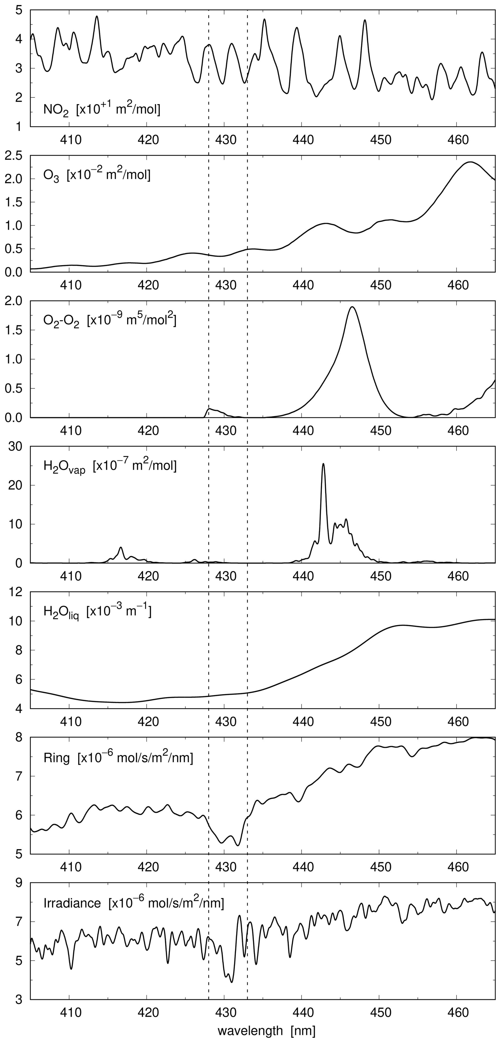
Figure 1 Convolved reference spectra used in the TROPOMI NO₂ SCD retrieval, Eq. (2), as well as the reference irradiance spectrum for detector row 225 within the fit window. The vertical dashed lines indicate wavelengths 428.0 and 433.0 nm. A description of these spectra, including references, is given in the NO₂ ATBDs of TROPOMI and OMI (van Geffen et al., 2025, 2026).

The DOAS retrieval then amounts to minimisation of the chi-squared merit function:

$$\begin{array}{}\text{(3)}& {\mathit{\chi }}^{\mathrm{2}}=\sum _{i=\mathrm{1}}^{n_{\mathit{\lambda }}}{\left({\displaystyle \frac{R_{\mathrm{resid}}\left({\mathit{\lambda }}_i\right)}{\mathrm{\Delta }{R}_{\mathrm{meas}}\left({\mathit{\lambda }}_i\right)}}\right)}^{\mathrm{2}}\end{array}$$

where R_resid(λ) is the so-called fit residual:

$$\begin{array}{}\text{(4)}& R_{\mathrm{resid}}\left(\mathit{\lambda }\right)=R_{\mathrm{meas}}\left(\mathit{\lambda }\right)-R_{\mathrm{mod}}\left(\mathit{\lambda }\right)\end{array}$$

n_λ is the number of wavelengths (spectral pixels) in the fit window (405–465 nm) and ΔR_meas(λ_i) is the uncertainty on the measured reflectance, which depends on the precision of the radiance and irradiance measurements as given in the level-1b product, i.e. on the signal-to-noise ratio (SNR) of the measurements (Kleipool et al., 2018; Ludewig et al., 2020). The χ²-minimisation is performed with an Optimal Estimation (OE; based on Rodgers, 2000) routine. For TROPOMI n_λ is 304 or 305, for OMI n_λ is 287 or 288, depending on the row. Both χ² and the root-mean-square (RMS) error of the fit:

$$\begin{array}{}\text{(5)}& R_{\mathrm{RMS}}=\sqrt{{\displaystyle \frac{\mathrm{1}}{n_{\mathit{\lambda }}}}\sum _{i=\mathrm{1}}^{n_{\mathit{\lambda }}}{\left(R_{\mathrm{resid}}\left({\mathit{\lambda }}_i\right)\right)}^{\mathrm{2}}}\end{array}$$

can be seen as a measure for the goodness of the fit, though both are continuous quantities, hence it is not possible to say where the separation between “good fit” and “bad fit” lies.

Spectral pixels are flagged in case they need to be removed from the fit due to problems encountered in producing the level-1b spectra (e.g. saturation, blooming, transients; Ludewig et al., 2020), the outlier removal routine included in the NO₂ DOAS retrieval (van Geffen et al., 2020, 2025, Appendix F), or deliberate removal of a section of the fit window, as suggested in this paper. The error on the reflectance of these flagged spectral pixels is set to 10⁴ times the measurement: ΔR_meas(λ_i) $={\mathrm{10}}^{\mathrm{4}}\times R_{\mathrm{meas}}\left({\mathit{\lambda }}_i\right)$, as a result of which they do not contribute to the residual in the χ²-minimisation, but the value of χ² will be lower due to the flagging, even if the rest of the residual would remain unchanged. In the computation of the RMS error in Eq. (5), however, the flagged pixels need to be skipped, lowering the n_λ therein.

If the DOAS retrieval does not converge or if the number of flagged spectral pixels is too large ($>\mathrm{1}/\mathrm{4}$-th of the fit window) or if the number of outliers found is too large (>10), the qa_value is set to zero. The OE retrieval provides an estimate of the uncertainties on (precision of) the fit parameters; if the NO₂ uncertainty is large (ΔN_s>33.0 µmol m⁻² $=\mathrm{2}\times {\mathrm{10}}^{\mathrm{15}}$ molec. cm⁻²), the qa_value is set to 0.15.

2.2.2 NO₂ slant column uncertainties

The DOAS uncertainty on the NO₂ SCD, ΔN_s, provided by the OE routine is an estimate that depends on details of the fit. The spatial variability of the SCDs over a remote Pacific Ocean sector can be used as an independent statistical estimate of the random component of the SCD uncertainty. Zara et al. (2018) used this approach to compare OMI and GOME-2A NO₂ and formaldehyde SCDs retrieved by different retrieval groups within the QA4ECV project, as well as to compare the SCD error estimates following from the different DOAS fits over the years 2005 through 2015. van Geffen et al. (2020) provided an initial analysis of TROPOMI NO₂ SCD uncertainties based on the then available data versions (v1.2.0 & v1.3.0) up to 31 January 2020.

As part of an ongoing monitoring of the stability of TROPOMI NO₂ retrievals, the DOAS and statistical uncertainties were recomputed after the mission reprocessing with data version v2.4.0 and is continued for subsequent versions manually on an irregular basis. To monitor the OMI NO₂ stability, preliminary collection 4 data (cf. Sect. 2.1.2) has been analysed as well, from the first available data of 1 October 2004 onwards up to end of 2025.

For each day the first available orbit with satellite (nadir viewing) equator crossings west of about −135° is selected as Pacific Ocean orbit (if such an orbit is missing on a given day, that day is skipped from the analysis) and analysed in the latitude range $[-\mathrm{60}\mathit{°}:+\mathrm{60}\mathit{°}]$: N_s and ΔN_s values are averaged in 2° × 2° grid cells, after which the average over these grid cells of the ΔN_s gives the DOAS uncertainty, while the standard deviation of the N_s over these grid cells gives the statistical uncertainty (following Zara et al., 2018, grid cells wherein the geometric AMF varies more than 5 % are discarded from the averaging, as are grid cells with less than 10 ground pixels in them). Results of this analysis, along with the monitoring of several other quantities, are presented on a set of web pages (see https://www.temis.nl/tropomi/no2scd/; last access: 15 June 2026).

Figure 2 shows a summary of the results: yearly average DOAS and statistical uncertainties for TROPOMI and OMI for clear-sky and cloud-free pixels separately. Per ground pixel the mean uncertainty of TROPOMI is significantly smaller then for OMI (due to the lower SNR of OMI) and on top of that the ground pixels are also much smaller. The pixel size reduction of TROPOMI on 6 August 2019 has lead to an increase of the uncertainties of about 10 % (van Geffen et al., 2020). After this size reduction there is a small increase in the TROPOMI uncertainties of on average 0.03 µmol m⁻² ($=\mathrm{2.0}\times {\mathrm{10}}^{\mathrm{12}}$ molec. cm⁻²) per year, while OMI uncertainties increase nearly five times faster: on average 0.14 µmol m⁻² ($=\mathrm{8.5}\times {\mathrm{10}}^{\mathrm{12}}$ molec. cm⁻²) per year.

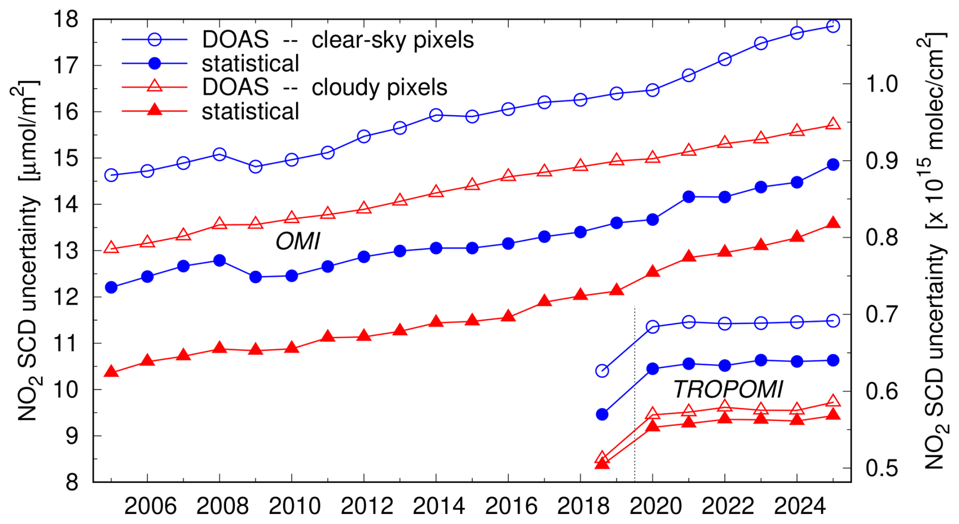
Figure 2 Yearly average DOAS (open symbols) and statistical (filled symbols) uncertainties for clear-sky (blue symbols) and cloudy (red symbols) pixels of the OMI (top four curves) and TROPOMI (bottom-right four curves) NO₂ slant column retrieval over the Pacific Ocean. In view of the TROPOMI pixel size reduction on 6 August 2019 (indicated by the vertical dotted line), the first year cannot be a calendar year; instead the period 1 August 2018 through 31 July 2019 is used.

As mentioned in Sect. 2.1.1, the improvement described in this paper is used in the operational TROPOMI processor since 22 November 2025, so that in fact the 2025 values shown in Fig. 2 are averages mixing two versions, but that is not a problem in view of the purpose of this figure since the improvement has only a small effect on the uncertainties; the TROPOMI data will be re-analysed after the forthcoming mission reprocessing (cf. Sect. 2.1.1). The OMI averages in Fig. 2 are determined from a preliminary version of the OMI collection 4 slant column data (OMNO2A) and thus not yet including the improvement discussed here; the final OMI collection 4 slant column data will be re-analysed at a later date.

2.2.3 The Wald-Wolfowitz runs test on the fit residual

TROPOMI observations over lakes in Tibet under clear-sky and snow-free circumstances revealed tropospheric NO₂ columns markedly larger than in the surrounding area. Kong et al. (2023) attributed these enhanced columns to unknown NO₂ sources in the lakes. This prompted us to investigate NO₂ fit residuals in detail and we noticed, as reported by Labzovskii et al. (2024), that these residuals contain clear broad-band structures that are likely an indication that the NO₂ SCDs retrieved over these lakes are unreliable: some kind of absorber present in the water is clearly not accounted for in the modelled refectance. A tell-tale sign in this case was also that the water vapour fit coefficients have large negative values (down to −1700 mol m⁻²) rather than positive values similar to those around the lakes (about +200 mol m⁻²). The issue found over these Tibetan lakes is revisited in Sect. 6.1.

The discovery of structures left in the fit residual prompted us to implement a statistical test to try to signal for remaining low frequency structures in the fit residual: the Wald-Wolfowitz runs test, or “runs test” for short (Barlow, 1989, Sect. 8.3.2; see also: https://en.wikipedia.org/wiki/Wald-Wolfowitz_runs_test, last access: 15 June 2026).

This test checks a randomness hypothesis based on the number of positive (k_p) and negative (k_n) values in the fit residual, i.e. based on the notion that an ideal fit residual is pure white noise, where a sequence of same-signed values is called a “run” and $n_{\mathit{\lambda }}=k_{\mathrm{p}}+k_{\mathrm{n}}$ the number of spectral points in the fit window. The number of expected runs, $k_{\mathrm{r}}^{\exp }$, the variance ${\mathit{\sigma }}_{\mathrm{r}}^{\mathrm{2}}$, and the deviation in terms of the standard deviation, R_D, are given by:

$$\begin{array}{}\text{(6)}& \begin{array}{rl}& k_{\mathrm{r}}^{\exp }=\mathrm{1}+\left(\mathrm{2}{k}_{\mathrm{p}}{k}_{\mathrm{n}}\right)/n_{\mathit{\lambda }}\\ & V\left(k_{\mathrm{r}}^{\exp }\right)={\mathit{\sigma }}_{\mathrm{r}}^{\mathrm{2}}=\left(\mathrm{2}{k}_{\mathrm{p}}{k}_{\mathrm{n}}(\mathrm{2}{k}_{\mathrm{p}}{k}_{\mathrm{n}}-n_{\mathit{\lambda }})\right)/\left(n_{\mathit{\lambda }}^{\mathrm{2}}(n_{\mathit{\lambda }}-\mathrm{1})\right)\\ & R_{\mathrm{D}}=\left(k_{\mathrm{r}}^{\mathrm{fit}\phantom{\mathrm{p}}}-k_{\mathrm{r}}^{\exp \phantom{\mathrm{f}}}\right)/{\mathit{\sigma }}_{\mathrm{r}}\end{array}\end{array}$$

where $k_{\mathrm{r}}^{\mathrm{fit}}$ is the number of runs in the fit residual. The deviation R_D has been defined here with a sign in order to make a distiction between fewer-than-expected (R_D<0) and more-than-expected (R_D>0) runs, i.e. to identify between low-frequency and high-frequency structures, respectively, in the fit residual. An additional quantity that proved to be useful is the length of the longest run, R_L, in the fit residual. See the ATBD (van Geffen et al., 2025) for further details and some examples.

An R_D that is $>+\mathrm{5}$ or $<-\mathrm{5}$ means that the number of runs is really in the tail of the distribution, while an R_L of, say, >20 is a significant fraction of the fit window. But since both R_D and R_L are continuous variables, it is not clear where to put a line between “good” and “bad” results. In addition, it is not certain that large R_D and R_L values actually mean that the retrieved NO₂ SCD is incorrect. And, vice versa, it is not certain that problems with the fit will always be picked up in the form of large R_D and/or R_L values. Still, both quantities can give useful information, which is why R_D and R_L are added to the TROPOMI NO₂ data product as additional independent information for the data user as of NO₂ data version v2.7.1.

3 Investigation of the fit residual issue

When looking at areas with large R_D and R_L, large patches over the oceans stood out clearly, prompting an investigation of fit residuals there, which in turn led us to the issue that is the subject of this paper. Initial investigations were done with TROPOMI orbits from 5 June 2019, as for that date the input data necessary for local reprocessing was available, since it was used for earlier investigations into the Tibetan Lakes issue (Sect. 6.1). Local reprocessing of (sections of) orbits was necessary, as the DOAS fit residual is not part of the nominal level-2 NO₂ files, since including residuals would lead to very large files while they would be of little use to by far most data users.

3.1 Atlantic Ocean

A section of orbit 08516 over the Atlantic Ocean (“atl” for short as id in figures and tables), with nadir latitudes $[+\mathrm{10}\mathit{°}:+\mathrm{40}\mathit{°}]$ was locally reprocessed so as to store the DOAS fit residuals and from this six clear-sky ground pixels with large R_L and large negative R_D were arbitrarily picked.

The top panel of Fig. 3 shows the fit residual from one example as a thin red line and a smoothed version of that as a thick red line. Results of the runs test for this fit residual are $R_{\mathrm{D}}=-\mathrm{6.3}$, i.e. really in the tail of the distribution, and R_L=33 (at $\mathit{\lambda }=[\mathrm{432.28}:\mathrm{436.58}]\mathrm{nm}$).

Atlantic Ocean fit residuals

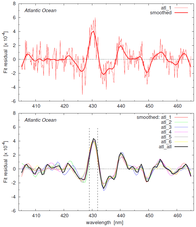
Figure 3 Examples of fit residuals of clear-sky pixels over the Atlantic Ocean (“atl” for short) that have large R_L and R_D. Top panel: residual of one example (thin red line) and the smoothed residual (thick red line). Bottom panel: smoothed residuals of six examples (thin lines) and a smoothed average of the six residuals (thick black line). Vertical dashed lines in the bottom panel indicate wavelengths 429.0 and 432.0 nm. Smoothing here and in other graphs is done with a natural spline without weights.

The bottom panel of Fig. 3 shows smoothed residuals of the six examples as thin lines and a smoothed average residual (“all”) as a thick line. All examples are around longitude −40°, latitude +26°; scanline and row numbers of these and of the other example pixels in this paper are listed in Appendix B.

Clearly noticeable in the fit residuals is the large peak around 430 nm. Both the RMS error and the χ² of the fit do not have suspiciously large values: those two quantities give no cause for alarm. Yet, the 430 nm peaks is clearly systematic and will have some impact on the NO₂ DOAS fit results.

To investigate the magnitude and occurence of this peak further, consider the ratio of the RMS of the peak – i.e. the wavelength range [429:432] nm, indicated in the bottom panel of Fig. 3, which spans about 15 spectral pixels – and the RMS of the rest of the fit window:

$$\begin{array}{}\text{(7)}& Q_{\mathrm{RMS}}^{\mathrm{430}}={\displaystyle \frac{R_{\mathrm{RMS}}(\mathit{\lambda }\in [\mathrm{429}:\mathrm{432}\left]\right)}{R_{\mathrm{RMS}}(\mathit{\lambda }\notin [\mathrm{429}:\mathrm{432}\left]\right)}}\end{array}$$

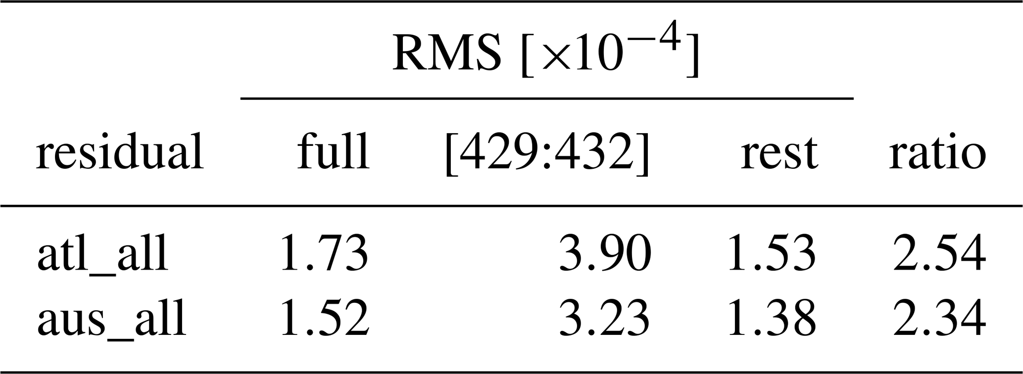
(Like the fit residual, this ratio is not part of the nominal level-2 files). The values of the RMS elements in Eq. (7) and the full-window RMS error of the average residual (“atl_all”) in Fig. 3 are given in Table 1; for the individual residuals the ratio varies between 2.3 and 2.8. The higher the ratio, the more pronounced the 430 nm peak stands out against the noise in the fit residual. Although RMS values are continuous quantities, a ratio $Q_{\mathrm{RMS}}^{\mathrm{430}}\ge \mathrm{2.0}$ likely indicates there is a problem with the NO₂ SCD.

Table 1 Residual RMS values over the full fit window (second column), the [429:432] nm range (third column), the remainder of the fit window (fourth column) and the $Q_{\mathrm{RMS}}^{\mathrm{430}}$ ratio (fifth column) of the average over the six clear-sky examples of the Atlantic Ocean (“atl_all”) in Fig. 3 and Western Australia (“aus_all”) in Fig. 5.

The top-left panel of Fig. 4 shows for the above mentioned orbit section the $Q_{\mathrm{RMS}}^{\mathrm{430}}$ ratio as function of the cloud radiance fraction: by far most pixels with a ratio ≥2.0 are clear-sky pixels (left part of the panel). In fact, the ratio is large only for clear-sky pixels for which the full-window RMS error of the fit is small. For these clear-sky pixels, where the satellite sees the ocean waters, the RMS_430 ratio increases with increasing value of the liquid water fit coefficient (top-right panel of Fig. 4): the deeper the light reaches into the ocean waters, the larger the effect of VRS on the retrieval and therefore the more pronounced the peak around 430 nm.

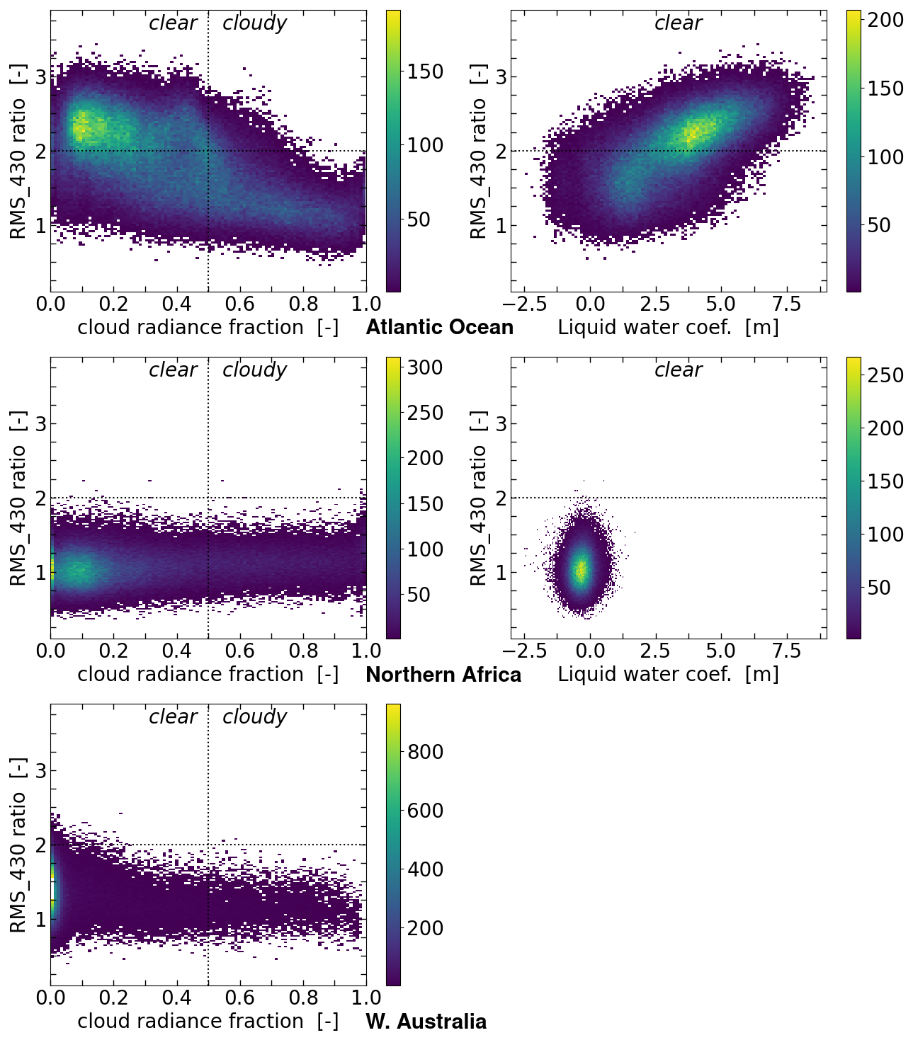
Figure 4 Scatter plots of the RMS_430 ratio (y axis) as function of the cloud radiance fraction (left column) and the liquid water fit coefficient for clear-sky pixels (right column) over the Atlantic Ocean (top row), Northern Africa (middle row) and Western Australia (bottom row). Horizontal dotted lines indicate a ratio of 2.0. The vertical line in the left column panels indicates the separation between clear-sky (left) and cloudy (right) pixels. Colour bars in scatter plots like this show the number of occurrences.

For pixels with higher cloud radiance fraction the RMS error of the fit is higher and the RMS_430 ratio is lower. In other words: for most cloudy pixels, any problem with the fit residual around 430 nm is possibly hidden between the larger noise on the residual due the presence of those clouds; the higher the cloud radiance fraction, the larger the range of RMS error values, i.e. of noisiness of the fit residual. The RMS_430 ratio does not show a dependency with either the solar or the viewing zenith angle, neither for clear-sky nor for cloudy pixels.

3.2 Northern Africa

For comparison of what goes on over land, consider a section of orbit 08514 over Northern Africa, with nadir latitudes $[+\mathrm{10}\mathit{°}:+\mathrm{30}\mathit{°}]$, which is slightly smaller than the Atlantic Ocean section used above to avoid including the Mediterranean Sea, but otherwise covers the same latitudes.

As the middle row of Fig. 4 shows, there are only a few pixels with $Q_{\mathrm{RMS}}^{\mathrm{430}}>\mathrm{1.5}$ (about 4 % from the orbit section), while the full-window RMS has roughly the same range as for the Atlantic Ocean section. Apparently there is no issue around 430 nm over this area of land. But this does not hold everywhere over land.

3.3 Western Australia

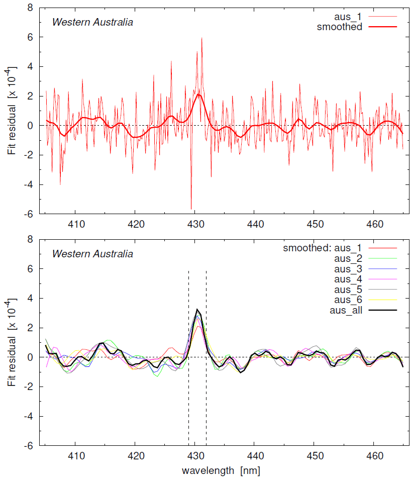
When inspecting other land areas where $Q_{\mathrm{RMS}}^{\mathrm{430}}>\mathrm{2.0}$ occurs in the 5 June 2019 orbits, several pixels stood out over Western Australia, though quite scattered. To look at this in more detail, consider the land pixels of a section of orbit 08510 with nadir latitudes $[-\mathrm{45.2}\mathit{°}:-\mathrm{7.5}\mathit{°}]$, which covers half of Australia west of about +135°, most of which is free of clouds.

The bottom-left panel of Fig. 4 shows the scatter plot of the RMS_430 ratio as function of the cloud radiance fraction: about 2 % of the really cloud-free pixels (i.e. with a very small cloud radiance fraction) have a ratio larger than 2.0, with a maximum of 2.43; for the Atlantic Ocean section the maximum ratio found is 3.45. None of the Australian land pixels is signaled by the runs test, with $\left|R_{\mathrm{D}}\right|<\mathrm{3.5}$ and R_L<20.

Figure 5 shows fit residuals of six ground pixels around longitude +120°, latitude −27° with RMS_430 ratios around 2.3; the bottom row of Table 1 lists the values of the RMS elements of Eq. (7) for the average (“aus_all”) over the six example residuals. There clearly is a peak around 430 nm that stands out above the noise in the fit residual, which definitely is not caused by VRS: the pixels are all classified as “shrubland”. Perhaps this indicates that the effect of RRS is not completely accounted for in the fit.

Figure 5 As Fig. 3 but for the clear-sky land pixels over Western Australia (“aus” for short) that have an RMS_430 ratio larger than 2.0.

3.4 RMS_430 ratio worldwide and change over time

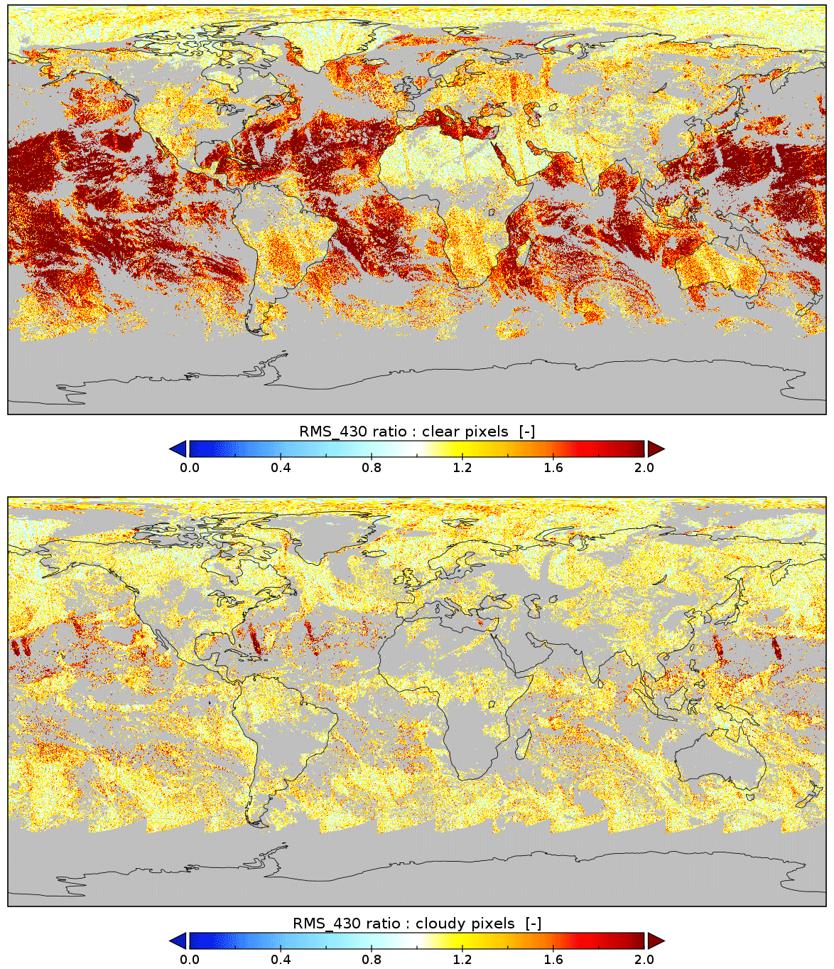
Figure 6 shows a map of the locations where $Q_{\mathrm{RMS}}^{\mathrm{430}}\ge \mathrm{2.0}$ for all TROPOMI orbits of 5 June 2019. Almost all these locations are over open water; over land there are only scattered pixels, as mentioned in the preceeding sections. Cloudy pixels tend to have a low RMS_430 ratio and therefore do not show up in the map. The outer 22 (20) rows at the left (right) edge of the swath have a larger spectral uncertainty, which is reflected in larger SCD and RMS errors, as a result of which the RMS_430 ratio is somewhat lower there.

Maps for other days (not shown) look similar, with a seasonal variation in the overall North-South pattern over the oceans and an apparent small decrease in time of the number of pixels with $Q_{\mathrm{RMS}}^{\mathrm{430}}\ge \mathrm{2.0}$. To investigate this further, Fig. 7 shows the frequency distribution of the RMS_430 ratio for cloud-free pixels of three selected days over water and over land separately.

From 5 June 2019 to 7 June 2020, the RMS_430 ratio decreases somewhat, clearly visible over water (blue lines) and less clearly over land (red lines). The reason for this decrease is likely the fact that due to the along-track pixel size reduction in August 2019 the uncertainties have increased (Sect. 2.2.2), i.e. the noise in the fit residual has increased, as a result of which the 430 nm peak stands out less clearly.

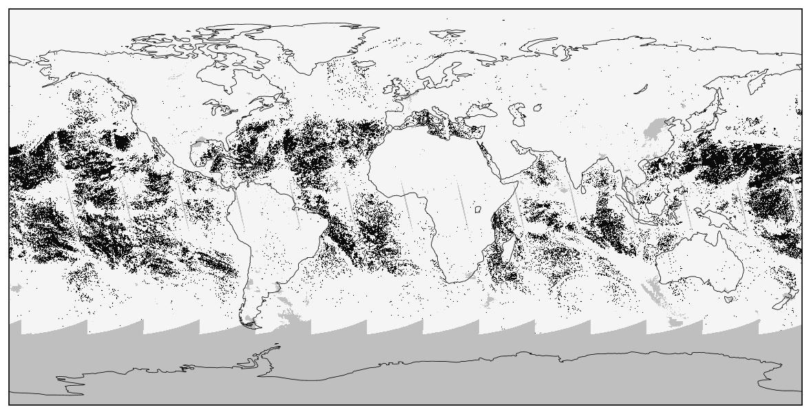
Figure 6 Map of ground pixels with $Q_{\mathrm{RMS}}^{\mathrm{430}}\ge \mathrm{2.0}$ in black and the other pixels in white from all orbits of 5 June 2019; a colour scale version of the map is given in Fig. C1 for clear-sky and cloudy pixels separately (Maps like this one are made with Panoply).

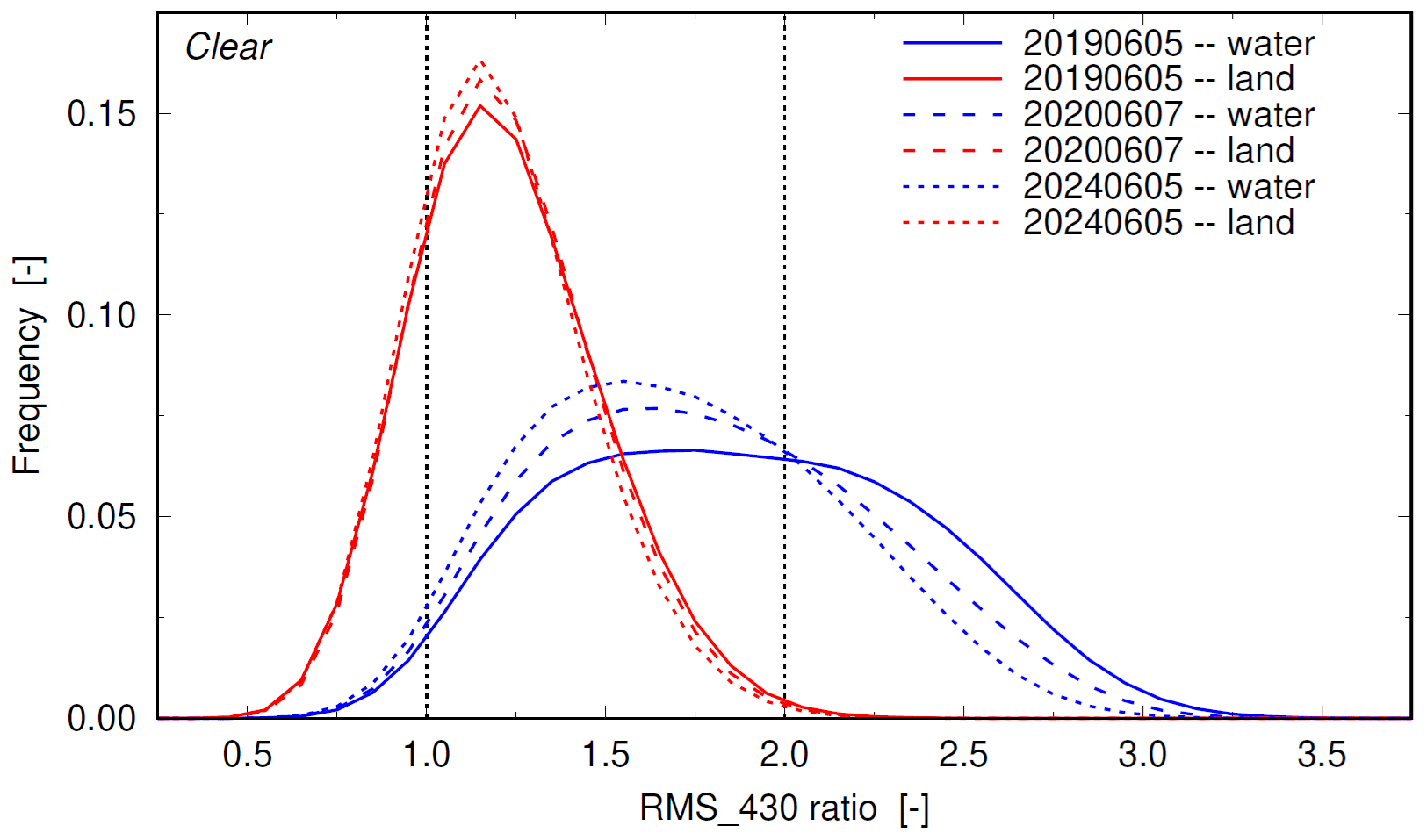
Figure 7 Frequency distribution of the RMS_430 ratio of all orbits of 5 June 2019 (solid lines), 7 June 2020 (dashed lines) and 5 June 2024 (dotted lines) for clear-sky pixels over water (blue) and land (red).

After that, the uncertainties of the NO₂ retrieval remain almost the same, as illustrated in Fig. 2, but Fig. 7 indicates that the 430 nm peak decreases in magnitude between 2020 and 2024, in particular over water but also over land. This is likely caused by the fact that in 2024 the Sun is more active than in 2020, as a result of which the 430 nm structure is less deep, in particular the calcium line there – see Appendix A for a brief investigation of the line depth over time. The irradiance and radiance are affected directly by the varying depth at that wavelength, while in addition to that the radiance over water is also indirectly affected by the change of the depth of the Ca+ lines around 395 nm which are shifted to around 430 nm by VRS (Sect. 1).

In other words: because the structure in the irradiance around 430 nm varies with the solar activity cycle, the effects of RRS are never really fully compensated around that wavelength, since the Ring reference spectrum (Sect. 2.2.1) is determined from a fixed irradiance reference spectrum, and over water things are made worse by the effects of VRS.

For ground pixels over clouds (not shown), the frequency distribution is slightly narrower than for the land pixels in Fig. 7, with a peak value at about the same RMS_430 ratio, also with a small narrowing over time and a small increase of the peak value.

3.5 OMI measurements

To investigate the RMS_430 ratio for OMI collection-4 measurements, Atlantic Ocean orbits similar to the TROPOMI one of 5 June 2019, where selected on or close to 5 June of 2005, 2009, 2014, 2019 and 2024.

Fit residuals of clear-sky pixels of the 5 June 2019 orbit (not shown) look very similar to those shown in Fig. 3, but on the whole the RMS_430 ratio is lower, the reason no doubt being that the noise on the OMI measurements is in general larger than on TROPOMI measurements: ratios above 2.5 are rare, most pixels have ratios well below 2.0, as can be seen from the red solid line in Fig. 8.

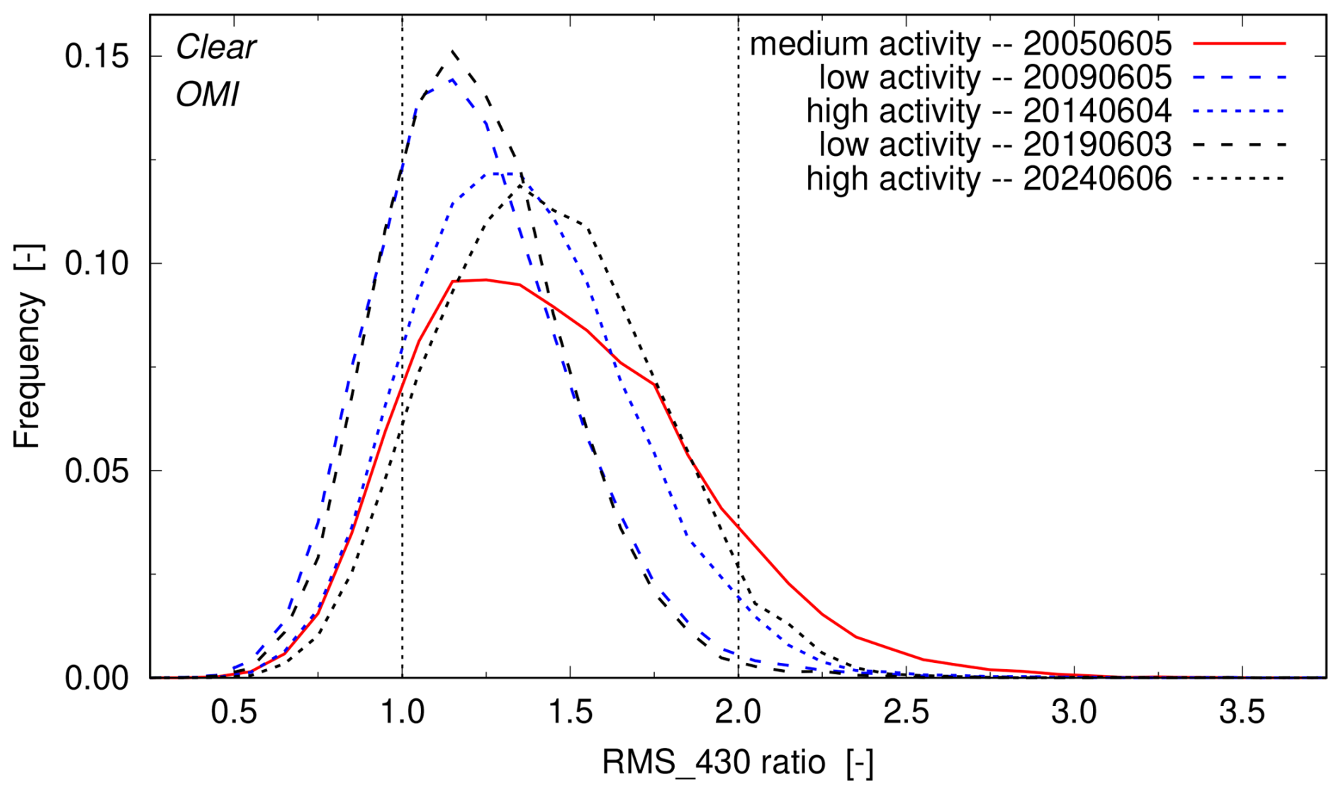
Figure 8 Frequency distribution of the RMS_430 ratio of clear-sky water pixels from OMI Atlantic Ocean orbits of five different years: 2005 with medium solar activity (solid red line), 2009 and 2019 with low solar activity (blue and black dashed lines), and 2014 and 2024 with high solar activity (blue and black dotted lines). Data affected by the row anomaly are filtered out; for consistency sake, the 2005 data have been filtered with the 2024 row anomaly flagging.

That figure also shows that the change over time of the RMS_430 ratio for OMI is quite different than for TROPOMI (cf. Fig. 7) in relation to the solar activity cycle: the higher activity of 2024 leads for TROPOMI to lower RMS_430 ratios than for the lower activity of 2020, while for OMI the higher activity of 2014 and 2024 (dotted lines in Fig. 8) leads to higher RMS_430 ratios than for the lower activity of 2009 and 2019 (dashed lines). The increase of the overall SCD error for OMI over time (Fig. 2) and thus of the RMS error, may be visible in Fig. 8 in the difference between the two low-activity (dashed) lines as a small shift to lower RMS_430 ratios, whereas in the two high-activity (dotted) lines it seems to show up as an small shift to higher RMS_430 ratios; these differences, however, could also be due to differences in atmospheric circumstances.

The reason for the different behaviour of TROPOMI and OMI is not clear, but it may be related to the fact that for OMI NO₂ retrievals the 2005 average irradiance is used, while for TROPOMI the daily measured irradiance is used (cf. Sect. 2.2.1), as a result of which the effect of the 430 nm issue on the reflectance and hence on the fit residual is quite different for the two instruments.

For cloudy pixels (not shown), the situation is more like TROPOMI: at low activity, the RMS_430 ratios are on the whole a little larger than at high activity.

4 Dealing with the fit residual issue at 430 nm

From the above analysis it is clear that around 430 nm there is a systematic feature that will have some impact on the NO₂ SCDs, in particular over oceans but also lands pixels may be affected. Compensating for this issue within the DOAS fit is not trivial as the feature appears to vary over time. Using the RMS_430 ratio of Eq. (7) as a filter is not possible either, as that ratio is a continuous quantity, like the χ² and RMS error of the fit.

We therefore propose to cut the feature from the DOAS fit by ignoring wavelengths in the range $\mathit{\lambda }=[\mathrm{428}:\mathrm{433}]\mathrm{nm}$, named “NO₂-gap fit” below. This window – slightly bigger than the range used in Eq. (7), to be sure to include the full feature – is indicated by the dashed vertical lines in Fig. 1. We recommend that this fix is implemented for all ground pixels, not just over ocean waters, to avoid introducing retrieval inconsistencies across land-water boundaries.

4.1 Individual pixel comparisons

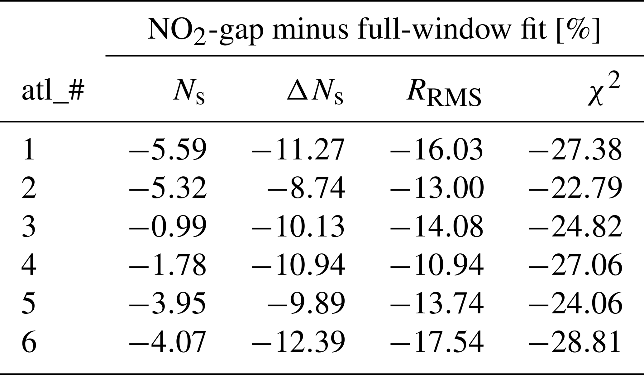
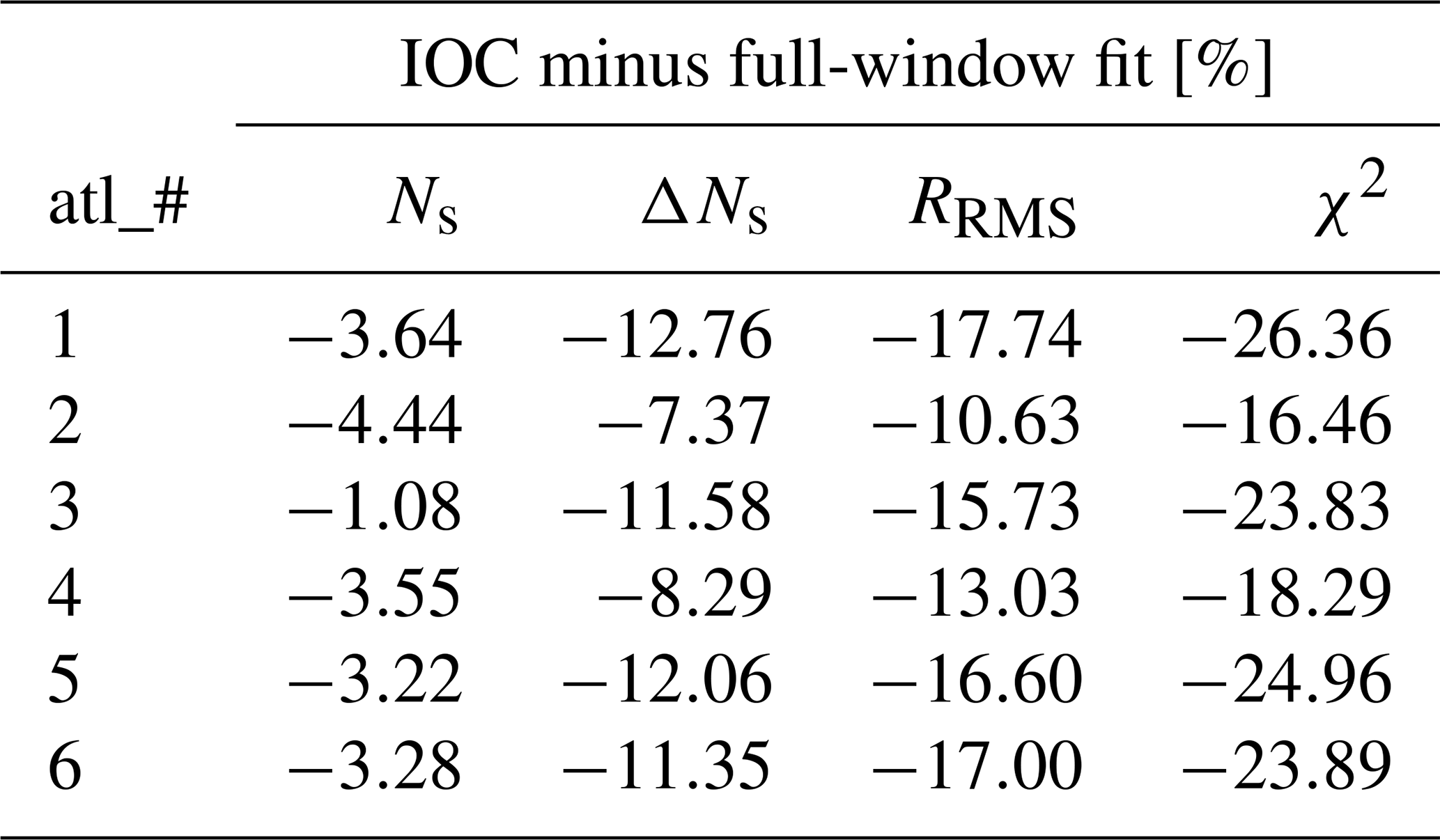
Figure 9 shows smoothed residuals of the Atlantic Ocean example from the top panel of Fig. 3 using the full-window fit (red line) and using the NO₂-gap fit (blue line): especially on either side of the gap the residual is reduced. Table 2 lists for the six Atlantic Ocean examples the change in the NO₂ SCD value, SCD error, RMS error and χ² of the fit. A reduction of the latter three – in these cases of 10 % or more – is generally considered to indicate that the fit has improved and one then assumes that the resulting SCD value has become more reliable.

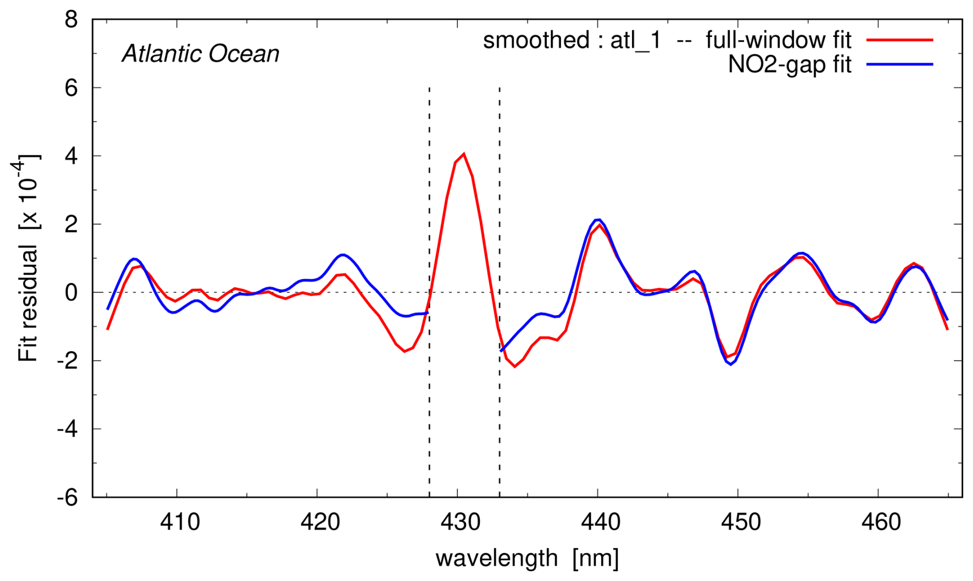
Figure 9 Smoothed fit residual of the Atlantic Ocean “atl_1” example in Fig. 3 using the full fit window for the retrieval (red line) and with the NO₂-gap fit (blue line). Vertical dashed lines indicate the wavelength range that is cut out: 428.0 to 433.0 nm.

Table 2 Changes in the main retrieval results between the NO₂-gap and the full-window fit in percent for the six clear-sky Atlantic Ocean pixels of Fig. 3.

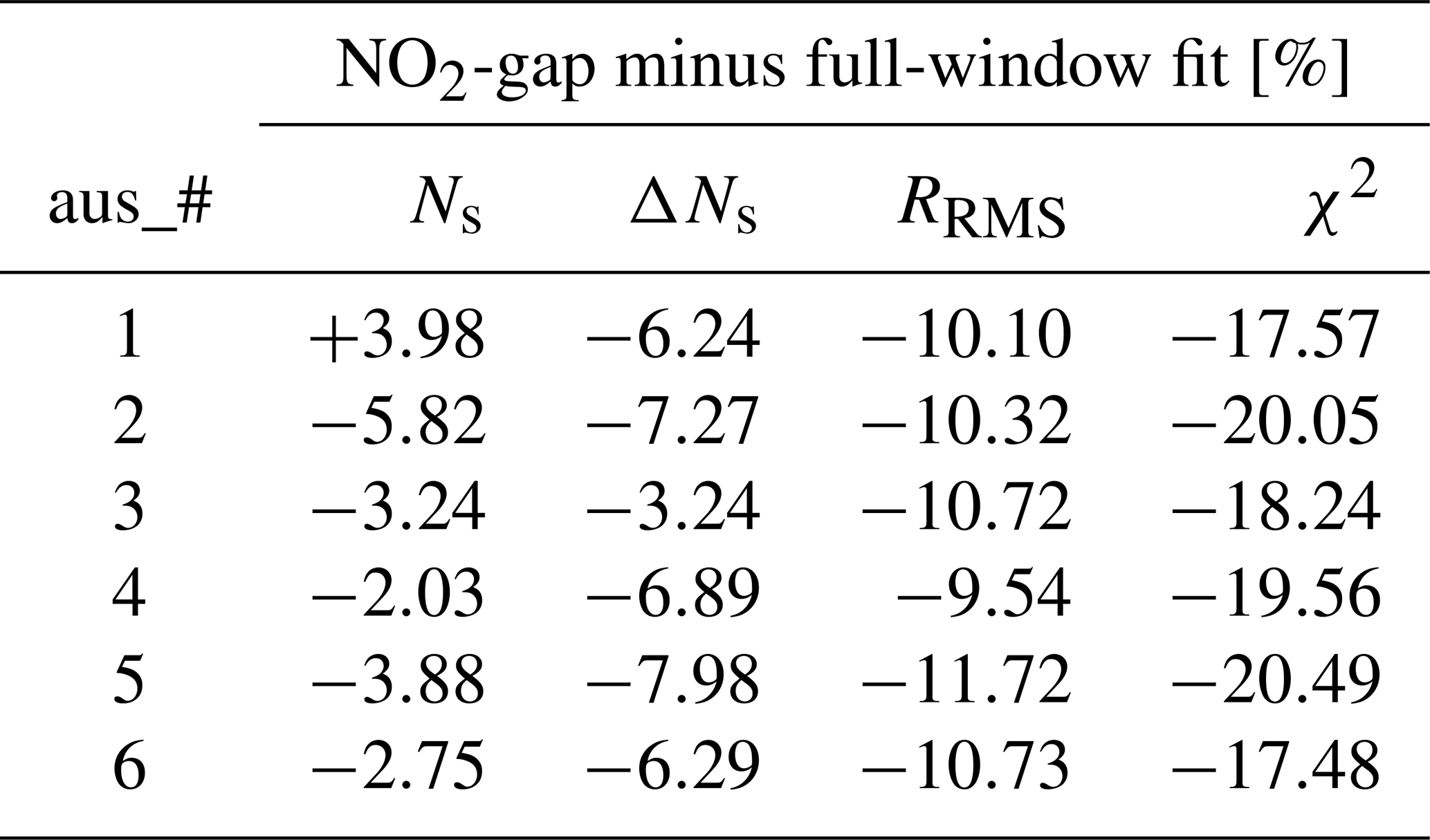
The NO₂-gap fit also leads to improved fits for the Western Australian land pixels, as can be seen from the results listed in Table 3, which shows that in some cases the SCD value may increase due to the improvements. For the Northern Africa land pixels (not shown), changes in the SCD and RMS error are for by far most pixels no more than ±2 %; for clear-sky pixels the changes are less than for cloudy pixels.

Table 3 As Table 2 but for the six clear-sky Western Australia pixels of Fig. 5.

4.2 Changes across the world and over time

Figure 10 shows a map of the relative change in percent of the NO₂ SCD error and the GCD value due to the NO₂-gap fit instead of the full-window fit for all orbits of 5 June 2019 – changes occur there where the RMS_430 ratio is large (cf. Fig. 6). Scatter plots of the changes in the NO₂ SCD error and GCD value are shown in Fig. 11 for clear-sky pixels over water and land and for all cloudy pixels, separately, as function of the RMS_430 ratio. For pixels over water, the reduction of the SCD error is evident, while over land there is also a decrease of the SCD error for a lot of pixels but some pixels show a small increase as result of the NO₂-gap fit. The GCD values show a small decrease over water, while over land they remain mostly the same. For cloudy pixels, the SCD error and GCD value changes are relatively small, where one has to keep in mind that for cloudy pixels with a cloud radiation fraction just above 0.5 part of the light still comes from the water or land surface.

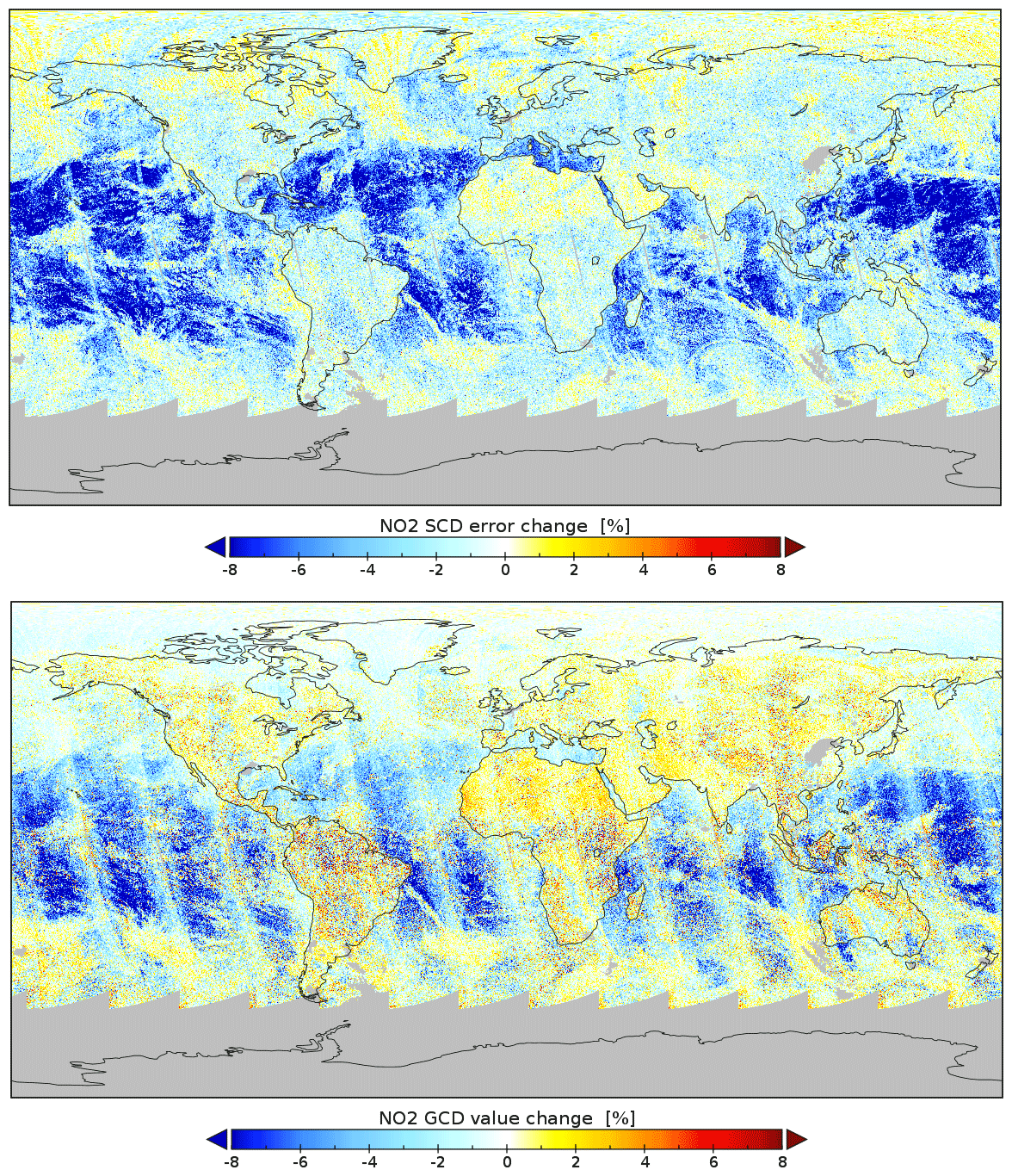
Figure 10 Map of the relative change in the NO₂ SCD error (top panel) and GCD value (bottom panel) of the NO₂-gap minus full-window fit for all orbits of 5 June 2019.

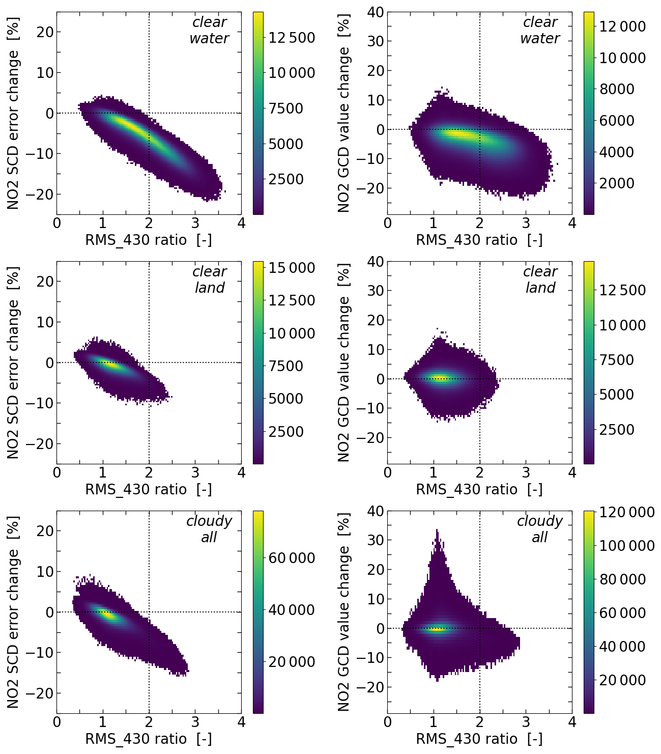
Figure 11 Scatter plots of the change in the NO₂ SCD error (left column) and GCD value (right column) of the NO₂-gap minus full-window fit in percent for clear-sky pixels over water (top row) and land (middle row), as well as all cloudy pixels (bottom row), of all orbits of 5 June 2019 as function of the RMS_430 ratio.

Frequency distributions of the changes for clear-sky pixels in the NO₂ SCD error and GCD value are shown by solid lines in Fig. 12, along with the changes for the other two test days mentioned above. The changes in the SCD error due to the NO₂-gap fit become a little smaller over time, along with what is seen for the RMS_430 ratio in Fig. 7, but on the whole there clearly is in improvement in the fit over water and a small improvement over land. The GCD value changes are more or less the same over time: a decrease over water and on average no change over land.

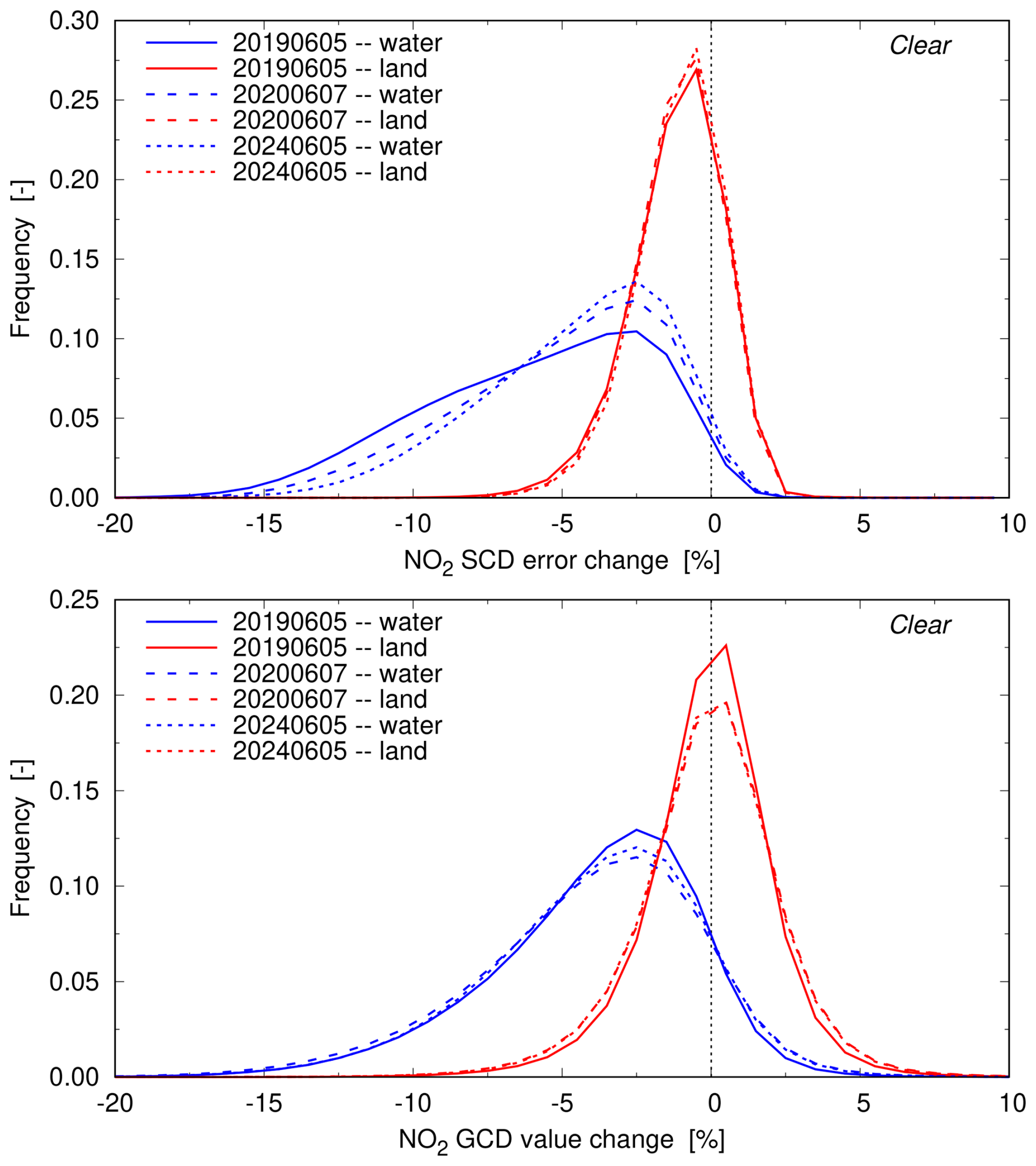
Figure 12 Frequency distribution of the NO₂ SCD error (top panel) and GCD value (bottom panel) of all orbits of 5 June 2019 (solid lines), 7 June 2020 (dashed lines) and 5 June 2024 (dotted lines) for clear-sky pixels over water (blue) and land (red).

For the initial evaluation of the impact of the NO₂-gap fit on the stratospheric and tropospheric columns, two full months were processed: July 2023 and January 2024 – see Sect. 5. The Pacific Ocean orbits of these two months can be used to check the impact on the slant column uncertainties discussed in Sect. 2.2.2. Given that there is quite some day-to-day variation, Table 4 lists the monthly average ratios of the uncertainties of the NO₂-gap over the full-window fit, as well as the average SCD value over the same latitude range (the difference between the two months is related to the seasonal cycle in the uncertainties; see the graphs on the webpages https://www.temis.nl/tropomi/no2scd/, last access: 15 June 2026).

Table 4 Monthly average ratio of the DOAS and statistical uncertainty (“unc.”) and the average SCD value of the NO₂-gap over full-window fit results of Pacific Ocean orbits of the two TROPOMI test months and for a period around the switch in the operation processor from v2.8.0 to v2.9.1 as specified in the text.

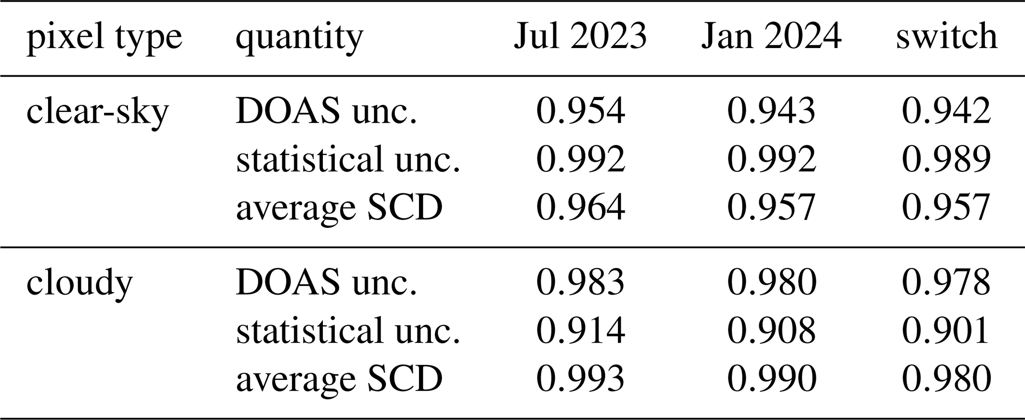
The NO₂-gap fit is included in the operational TROPOMI processor since 22 November 2025 (cf. Sect. 2.1.1), hence we can compare results after that up to what is available at the moment of writing, i.e. up to 30 April 2026, with v2.8.0 data of the same 160-d period one year earlier. The ratios of the averages over these two periods, listed in the last column of Table 4, agree quite well with those of the two test months.

As expected from the above reported changes in the SCD error, the DOAS uncertainty improves, in particular for clear-sky scenes. For those scenes the statistical uncertainty does not change much, but the NO₂-gap fit appears to have an impact on the statistical uncertainty over cloudy scenes with changes up to −10 %. It is not fully clear why the latter decrease occurs. As the bottom-right panel in Fig. 11 shows, the GCD does on average not change over clouds, but there is quite some scatter, even for low RMS_430 ratio. In particular over bright clouds and at edges of clouds the illumination of the instrument slit may be inhomogeneous, which is likely to have greatest effect on strong Fraunhofer lines. Perhaps the removal of the 430 nm peak therefore gives better, more consistent results over clouds due to the incomplete handling of that peak by the Ring correction in the full-window retrieval. The main message, though, is that the NO₂-gap approach reduces the uncertainties, in some cases more than in other cases, without a deterioration of the results.

4.3 OMI measurements

Inspecting OMI fit residuals of individual clear-sky Atlantic Ocean pixels with a relatively high RMS_430 ratio of the 2005 orbit without and with the NO₂-gap leads to graphs similar to Fig. 9 and the changes in the SCD and RMS error are of the same order as those listed in Table 2. For pixels from the 2024 orbit the changes in the SCD and RMS error appear to be smaller, probably because the 430 nm peak is relatively less strong in 2024 than in 2005 due to the increased solar activity (Sect. 3.5) and/or the increased measurement uncertainties (Sect. 2.2.2).

An evaluation of the data for water pixels only in the latitude range $[-\mathrm{40}\mathit{°}:+\mathrm{40}\mathit{°}]$, which covers the area where the largest changes are expected to occur, and filtering out the rows suffering from the row anomaly (also for the 2005 data, to have equal viewing geometry coverage), reveals that for most pixels the NO₂ SCD error is reduced in the NO₂-gap approach: the changes lie roughly between −12 % and +2 %. For clear-sky pixels the distribution of the SCD error changes peaks at about −0.5 % for the orbits of 2009 and 2019, i.e. when solar activity is low, with a frequency a 10th of the peak-frequency for a change of −5.5 %. For the high-activity years 2014 and 2024 the peak of the distribution lies at about −1.5 % and a frequency a 10th of the peak-frequency is found for a change of −9 %. For the 2005 orbit, a year of medium solar activity, the peak lies at roughly the same change but the tail is somewhat longer: a frequency a 10th of the peak-frequency is found at −10 %. In other words, for low-activity years the SCD error changes of clear-sky pixels have a narrower distribution than for high-activity years. The reverse is the case for cloudy pixels, and for these pixels the peaks lie between −1.5 % and −0.5 % for all years.

The changes of GCD values for these Atlantic Ocean pixels (which in general have low GCD values to begin with) have a wide distribution, roughly between −15 % and +10 % for most clear-sky pixels, with a peak at about −0.5 %, with only a little difference between low- and high-activity years. For cloudy pixels the GCD appears to increase a little on average: the changes range from about −10 % to +15 %, with peaks around +1 % to +2 %.

5 Impact on stratospheric and tropospheric columns

To study the impact of the NO₂-gap approach on the final stratospheric and tropospheric NO₂ columns two months were selected: July 2023 and January 2024, so as to capture seasonal variation. Since the TM5 data assimilation was started from an existing distribution and the across-track stripe correction amplitude is an average over a period of seven days (van Geffen et al., 2025), it takes a few days to adjust (spin-up) to new approaches, hence we analyse the vertical column data starting at day 8 of each month; the stripe correction amplitude is determined and applied after the SCD and GCD are calculated, and it may be different for the full-window and the NO₂-gap approaches. NO₂ column data were gridded per day using the HARP software (https://stcorp.github.io/harp/doc/html/; last access: 15 June 2026) on 0.2° × 0.2°, which gives average values where orbits overlap.

5.1 Overall impact

Since most of the NO₂ over the oceans, away from emission sources, is found in the stratosphere, a change in the SCD in those regions will primarily lead to changes in stratospheric NO₂. For the vast majority of the grid cells the change of the stratospheric column is in the range −5 % (−2 µmol m⁻² or 1.2×10¹⁴ molec. cm⁻²) to 0 %; cf. the top panel of Fig. 13. For some individual grid cells the changes may be a bit larger, while for very few grid cells stratospheric NO₂ may increase a little. Most of the change is found in the latitude range $[-\mathrm{40}\mathit{°}:+\mathrm{40}\mathit{°}]$, the same range where the largest changes in SCD and SCD error occur.

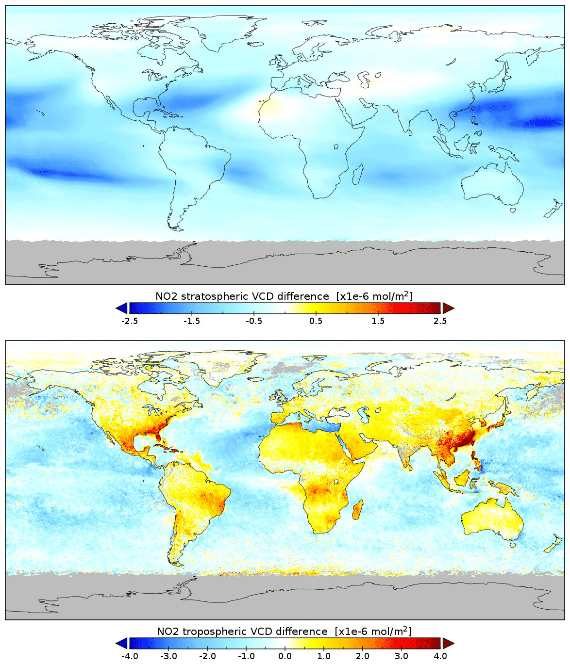
Figure 13 Average change NO₂-gap minus full-window in the stratospheric (top panel; all pixels) and tropospheric (bottom panel; clear-sky pixels only) NO₂ vertical column for the test month July 2023. The two panels have different scale ranges, both in µmol m⁻², where 4 µmol m⁻² corresponds to 2.4×10¹⁴ molec. cm⁻².

Since tropospheric NO₂ column values over oceans are usually small and over land they can vary quite a bit, it is best just to consider absolute differences; cf. the bottom panel of Fig. 13. For by far most clear-sky water grid cells the tropospheric column decreases: average changes are between −2.0 and +0.5 µmol m⁻², with a peak around −1.0 µmol m⁻². Clear-sky land scenes and all cloudy scenes, on the other hand, show an overall increase of the tropospheric column: average changes are between −0.5 and +2.0 µmol m⁻². Some individual grid cells show much larger (monthly average) changes though: between −20 and +15 µmol m⁻² for clear-sky scenes, while for cloudy scenes the changes may range between −40 and +40 µmol m⁻² (2.4×10¹⁵ molec. cm⁻²).

On average we expect that the impact on tropospheric columns is small, since the data assimilation will remove average biases. The lower stratospheric columns above tropical seas are transported over land, as is particularly visible over Eastern Asia and over South-East USA and Mexico (top panel of Fig. 13), where tropospheric columns will increase since the SCD over land remains more or less the same. Since over polluted areas the AMF is much smaller than the stratospheric NO₂, tropospheric columns may increase more than the stratospheric columns decrease. The data assimilation with the NO₂-gap retrieval results reduces the entire column over oceans, leading to a small decrease of the tropospheric columns there.

5.2 Impact over validation stations

Routine validation of TROPOMI tropospheric, stratospheric and total column data with ground-based measurements is being carried out by the Validation Data Analysis Facility (VDAF, https://mpc-vdaf.tropomi.eu/; last access: 15 June 2026), with support from the S5P Validation Team (S5PVT), which issues Quarterly Validation Reports, such as Lambert et al. (2026).

The VDAF data of a given station could be compared to the new results by selecting the same ground pixel from the orbit files, as a repetition of the validation. But that probably does not provide clear answers, given that (a) ground-based measurements are not available on each day of the two months, (b) in view of the spin-up the first seven days of each months need to be skipped, and (c) a large day-to-day variation is observed in the validation results, which is larger than the differences discussed here. Instead it seems a better idea to considered the data from the full-window and NO₂-gap retrievals at the VDAF locations in the gridded data.

The results of this comparison are shown in Fig. 14 in the form of monthly averages of daily absolute differences, where vertical dashed lines separate the three groups of stations for the validation of the stratospheric (15 locations; left), total (75 locations; middle) and tropospheric (8 locations; right) column; a few locations at high latitudes have no data in the local winter month.

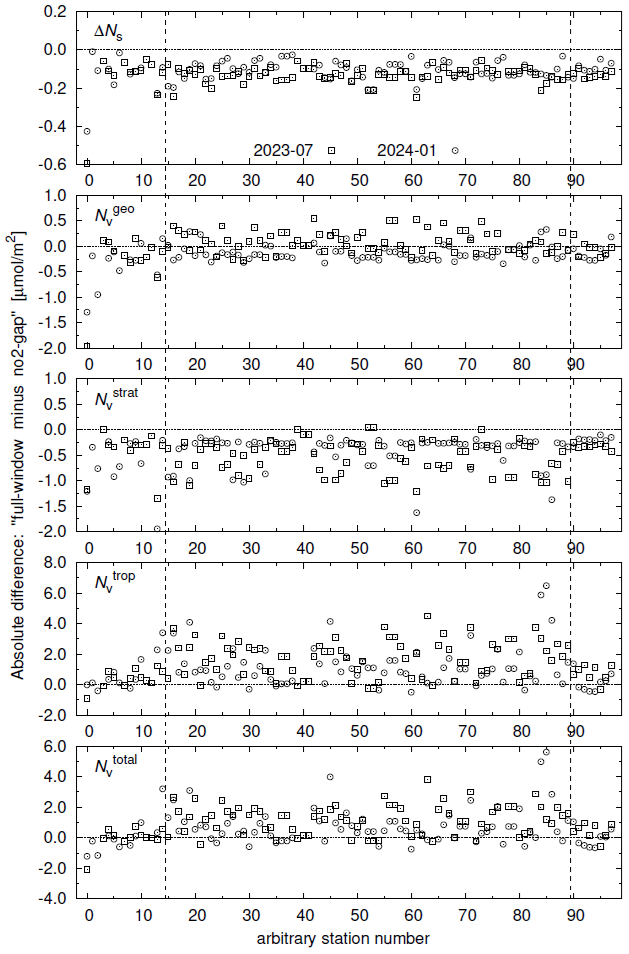
Figure 14 Average absolute change of, from top to bottom, the NO₂ slant column error (ΔN_s) and the geometric ($N_{\mathrm{v}}^{\mathrm{geo}}$), the stratospheric ($N_{\mathrm{v}}^{\mathrm{strat}}$), the tropospheric ($N_{\mathrm{v}}^{\mathrm{trop}}$) and the total ($N_{\mathrm{v}}^{\mathrm{total}}$) vertical columns between the NO₂-gap and the full-window fit results for the two test months over the VDAF validation sites for the 15 stratospheric (left part of each panel), 75 total (middle part) and 8 tropospheric (right part) columns. Stations have been assigned numbers in alphabethical order per group; the groups are separated by vertical dashed lines.

For most locations, the average SCD error (ΔN_s; top panel) is reduced by about 0.1 µmol m⁻² (0.6×10¹³ molec. cm⁻²) or about 1 %; the standard deviation of the averaging is smaller than the average for most stations. These reductions are quite small, because the stations are located on land, where the impact of the NO₂-gap approach is small. The largest change in ΔN_s occurs for the first stratospheric column station (Bauru, Brazil): −0.6 (−0.4) µmol m⁻² for the month July 2023 (January 2024), or −5.8 % and −3.7 %, respectively.

For that station, the average GCD column ($N_{\mathrm{v}}^{\mathrm{geo}}$; 2nd panel) goes down by 2.0 (1.3) µmol m⁻² in July 2023 (January 2024), or about −3.3 % for both months, while the third stratospheric column station (Dumont d'Urville, Antartica) shows a decrease of $N_{\mathrm{v}}^{\mathrm{geo}}$ by 1.3 µmol m⁻² in January 2024. For most other stations, the change in $N_{\mathrm{v}}^{\mathrm{geo}}$ is between −1 % and +1 %.

The average stratospheric column ($N_{\mathrm{v}}^{\mathrm{strat}}$; 3rd panel) decreases for almost all stations, from −0.2 to −1.0 µmol m⁻² (0.6×10¹⁴ molec. cm⁻², or up to −2 %), with a standard deviation lower than 0.3 µmol m⁻², i.e. the decrease of $N_{\mathrm{v}}^{\mathrm{strat}}$ is fairly robust. The 14th stratospheric column station (St. Denis, Reúnion) shows the largest decrease: −1.9 µmol m⁻² in January 2024 (about −4.5 %), followed by the 47th total column station (Mauna Loa, Hawaï): −1.6 µmol m⁻² in January 2024 (about −5.1 %). As the routine validation mentioned above shows, TROPOMI slightly underestimates the stratospheric column, but those results are latitude dependent. with a possible small overestimation in the tropics where the NO₂-gap approach is most prominent. It looks like the NO₂-gap approach reduces the latitude dependency a little, but the impact on the biases is difficult to estimate in view of the large uncertainties in the validation comparisons.

The average tropospheric column ($N_{\mathrm{v}}^{\mathrm{trop}}$; 4th panel) of the MAX-DOAS stations – all of which lie on the Northern hemisphere – does not change much and the same holds for most of the stratospheric column stations. For the total column stations the change of $N_{\mathrm{v}}^{\mathrm{trop}}$ has a quite varied distribution, with little to no change for some locations and changes +4.0 to +6.0 µmol m⁻² (3.6×10¹⁴ molec. cm⁻²) for other locations. Given that the tropospheric column values for some stations are small, relative changes can be large, but for most stations the relative change is less than ±15 %.

The average total column ($N_{\mathrm{v}}^{\mathrm{total}}$; 5th panel), i.e. the sum of the tropospheric and total column, shows changes similar to those in the $N_{\mathrm{v}}^{\mathrm{trop}}$.

All in all the changes in the vertical columns are on average small and are not likely to affect the main conclusions of the VDAF validation reports.

6 Discussion points

6.1 Tibetan lakes

As mentioned at the beginning of Sect. 2.2.3, unexpectedly large TROPOMI tropospheric NO₂ columns over Tibetan lakes, attributed by Kong et al. (2023) to sources in those lakes, are likely due to unreliable NO₂ slant column retrievals (Labzovskii et al., 2024), as indicated by the presence of broad-band structures in the fit residuals and large negative water vapour (H₂O_vap) coefficients over those lakes. For that study, orbit 08511 of 5 June 2019 was selected – the first orbit in June 2019 that has fully clear-sky pixels over two major lakes: Lake Siling and Lake Nam, but also other lakes in and around Tibet were investigated. For this paper, we focus on those two large lakes (located at about 4.5–4.7 km altitude), as well as on Issyk-Kul in Kyrgyzstan (at about 1.6 km altitude), as these cover multiple TROPOMI ground pixels.

The top panel of Fig. 15 shows the fit residual of a pixel over Lake Siling. Like the residuals over the Atlantic Ocean, shown in Fig. 3, there are broad-band structures in the residual above about 430 nm, but there are striking differences: the peak around 430 nm that lead to the NO₂-gap approach is much less pronounced here, the “downward wave top” between 430 and 440 nm is much deeper, and there is a strong negative “peak” at about 442.7 nm (indicated by an arrow). That peak can be attributed to the fact that the DOAS fit has, in order to minimise the residual, among others resulted in a strongly negative H₂O_vap coefficient of $-\mathrm{1.419}\pm \mathrm{0.280}\times {\mathrm{10}}^{\mathrm{3}}\mathrm{mol}{\mathrm{m}}^{-\mathrm{2}}$ for this example, as opposed to an average of $+\mathrm{0.235}\times {\mathrm{10}}^{\mathrm{3}}\mathrm{mol}{\mathrm{m}}^{-\mathrm{2}}$ outside the lake.

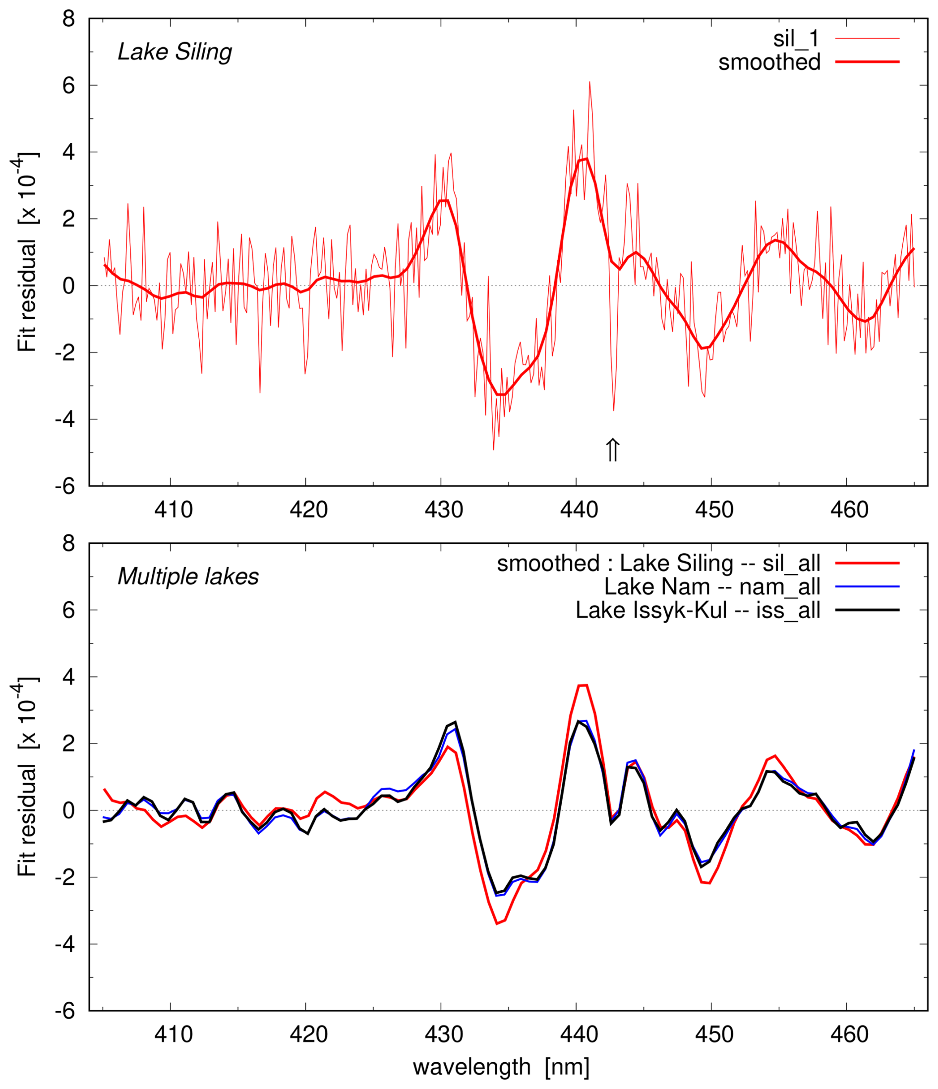
Figure 15 Top panel: example of a fit residual over Lake Siling (thin red line) and the smoothed residual (thick red line). The arrow at 442.7 nm points to an issue discussed in the text. Bottom panel: smoothed fit residuals of the average over six residuals over three lakes: Lake Siling (red line), Lake Nam (blue line) and Lake Issyk-Kul (black line) from the full-window fit; the blue and black lines almost exactly overlap.

Both the broad-band structures and the large negative H₂O_vap coefficient were tell-tale signs to conclude that the higher GCD values over the lakes (0.71 µmol m⁻² on average), compared to surrounding values (0.66 µmol m⁻² on average; cf. the maps in Labzovskii et al., 2024), are probably due to unrealiable fit results rather than due to NO₂ emissions from the lakes: since stratospheric NO₂ is more or less constant over the short distances involved here, any elevation in the retrieved SCD value will end up as an enhancement of the tropospheric NO₂ column.

Residuals of other ground pixels over Lake Siling, Lake Nam and Lake Issyk-Kul look similar, with some difference in the details of the broad-band structures and the H₂O_vap values. The bottom panel of Fig. 15 shows for the three lakes the smoothed fit residual averaged over six ground pixels with surface classification “Water” – even in these smoothed versions, the downward peak related to the negative H₂O_vap coefficient can be seen.

The broad-band structure between 430 and 440 nm is picked up by the runs test: R_L>20, as is visible in the maps on the top row of Fig. 16, and $R_{\mathrm{D}}<-\mathrm{5}$ for most pixels. For Lake Siling, the RMS_430 peak is barely visible, while for Lake Nam and Lake Issyk-Kul part of the water pixels have $Q_{\mathrm{RMS}}^{\mathrm{430}}\ge \mathrm{2.0}$ (red patches in the bottom row maps of Fig. 16).

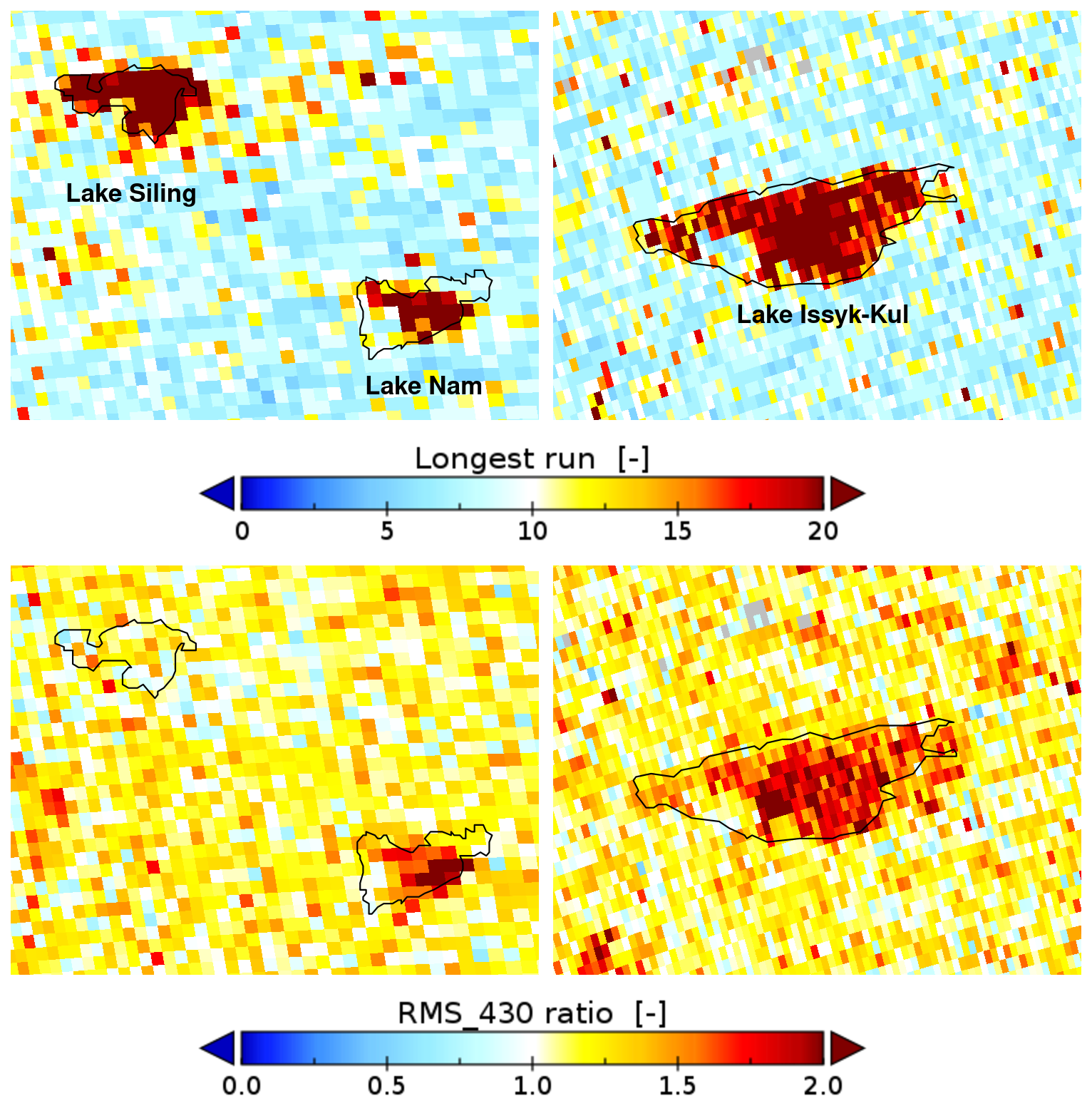
Figure 16 Maps of the longest run R_L (top row) and RMS_430 ratio (bottom row) for Lakes Siling and Nam (left column; centred at +89.8°, +31.2°) and Lake Issyk-Kul (right column; centred at +77.4°, +42.5°). Maps are 2° in north-south direction. Approximate lake contours are made by Panoply.

The lower RMS_430 ratio over these lakes as opposed to the ratio over the Atlantic Ocean indicates that for the lakes the effects of VRS are less important and in some cases apparently absent. Liquid water fit coefficients over the Atlantic Ocean are usually around several metres (cf. top-right panel of Fig. 4), whereas for Lake Siling and Lake Issyk-Kul they are around +1 m, while Lake Nam has values around −3.5 m; the latter is another indication that the DOAS fit is not really going well here. Differences in the overall broad-band structures in the fit residual may be due to the fact that the characteristics of the material dissolved in the water of the lakes differs from what is dissolved in the oceans.

Looking at results for the three lakes when using the NO₂-gap fit introduced above reveals that for Lake Siling the changes are small and erratic: for some pixels the RMS and SCD error and the GCD value go down by one or two percent, while for other lake pixels they go up a little. For Lakes Nam and Issyk-Kul, the RMS and SCD error appears to go down by five to ten percent, and the GCD value by one to four percent. In other words, the NO₂-gap approach improves the fit quality somewhat but does not solve the issue of the observed bias in the slant column values over these lakes. To solve the bias additional reference spectra, describing the characteristings of the material dissolved in lakes, need to be added to the fit, but such spectra are currently not known.

6.2 Intensity offset correction

Several DOAS applications include an intensity offset correction (IOC for short), constant or linear in wavelength, to improve the retrievals in some spectral ranges. This correction has been implemented in the TROPOMI NO₂ processor in the form of an addional term to Eq. (2):

$$\begin{array}{}\text{(8)}& R_{\mathrm{mod}}\left(\mathit{\lambda }\right)=\mathrm{\dots }+{\displaystyle \frac{\sum c_m{\mathit{\lambda }}^m}{E_{\mathrm{0}}\left(\mathit{\lambda }\right)}},m=\mathrm{0},\mathrm{1},\mathrm{\dots },n_{\mathrm{off}}\end{array}$$

with c_m fit parameters; in most applications n_off=0 or 1. The option has, however, not been turned on, mainly because the precise physical origin of such an intensity offset is not known – it is thought to be related to instrumental issues (e.g. incomplete removal of stray light or dark current in Level-1b spectra, neither of which is deemed necessary for TROPOMI measurements) and/or atmospheric issues (e.g. incomplete removal of Ring spectrum structures and VRS in clear ocean waters); see, for example, Platt and Stutz (2008), Richter et al. (2011), Lampel et al. (2015), Boersma et al. (2018).

The blue line in Fig. 17 shows the smoothed fit residual in case the IOC is turned on in the full-window fit with n_off=0: the IOC clearly decreases the 430 nm issue and gives close to it a slightly better fit residual, quite similar to the NO₂-gap fit (black dotted line); the shape of the IOC term is indicated by the thin grey line at the bottom of the panel. The change in the NO₂ SCD value, SCD error, RMS error and χ² for the six Atlantic Ocean example pixels are listed in Table 5 – these changes are similar to but somewhat less than those for the NO₂-gap fit listed in Table 2.

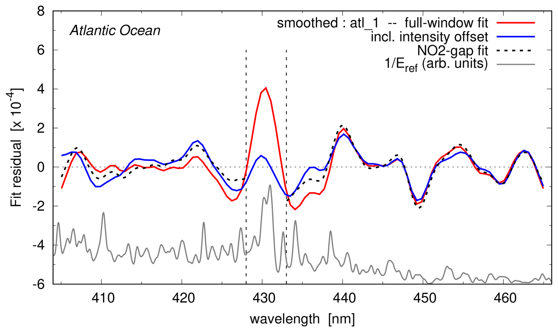
Figure 17 Smoothed fit residual of the Atlantic Ocean “atl_1” example in Fig. 3 using the full fit window for the retrieval without (red line) and with (blue line) the IOC, and with the NO₂-gap fit (black dotted line). The thin grey line at the bottom is $\mathrm{1}/E_{\mathrm{ref}}$ in arbitrary units (cf. bottom panel in Fig. 1), indicative of the shape of the IOC term.

Table 5 Changes in the main retrieval results in percent for the six clear-sky Atlantic Ocean pixels of Fig. 3 due to the intensity offset correction (IOC).

The IOC is proportional to one over the irradiance and the Fraunhofer peak in the irradiance is much narrower than the 430 nm residual issue, hence the IOC can never fully compensate for the issue. In addition to that, the $\mathrm{1}/E_{\mathrm{0}}\left(\mathit{\lambda }\right)$ spectrum has additional structures and shows a slope above 440 nm, which may be introducing artifacts in the retrieval.

All things considering, the NO₂-gap fit seems to be a physically better justifiable approach than including the IOC in the fit to solve the 430 nm issue. Neither of the two approaches, however, are able to deal with the broad-band structures at higher wavelengths.

6.3 Chlorophyll and other material in the water

The NO₂-gap fit was introduced to remove the systematic residual feature around 430 nm. This does not deal with issues at higher wavelengths visible in the fit residuals (e.g. Fig. 9), which are related on the one hand to wavelength shifts caused by VRS effects (Peters et al., 2014; Dinter et al., 2015; Holtrop et al., 2021) and on the other hand by the presence in the water of, for example, chlorophyll and dissolved organic matter (DOM), which are known to absorb light in the visible region (Joiner et al., 2004; Cannizzaro and Carder, 2006; Vountas et al., 2007), and particulate matter that may be scattering UV radiation. Chrolophyll and DOM come in different flavours, each with their own slightly different reference spectrum (Taniguchi et al., 2021). It is unclear whether these structures remaining in the fit residual mean that the retrieved NO₂ SCD is affected, but the results of the lakes discussed in Sect. 6.1 suggest they may well be.

The broad-band structures visible in the fit residual themselves do not represent the missing reference spectrum, because the shape of the residual is the result of DOAS adjusting all fit parameters so as to minimise the residual, i.e. possibly using incorrect fit coefficients – cf. the downward peak in Fig. 15 due to the large negative water vapour coefficient. Note further that the reference spectra σ_k(λ) are in the exponent of the modelled reflectance of Eq. (2), rather than directly in the residual.

Over relatively small areas like the lakes in Sect. 6.1, where one may assume the stratosphere to be more or less constant, one could try to reconstruct the missing reference spectrum by assuming that the fit coefficients found outside the lake are valid over the lake as well, with some sensible assumption of what the liquid water coefficient might be, although it is then unclear what one should assume for the polynomial coefficients. An attempt in that direction falls outside the scope of the present paper. In addition, the approach would not work over oceans, as there are no neighbouring values for the fit coefficients available.

7 Concluding remarks

The first step in the process to determine NO₂ tropospheric and stratospheric columns from measurements by satellite-based instruments, such as TROPOMI, is the retrieval of the so-called slant column density (SCD) of NO₂ with a DOAS approach, in the case of TROPOMI NO₂ in the wavelength window 405–465 nm. This retrieval step accounts for the presence of several absorption and scattering effects that occur along the light path from Sun through atmosphere to satellite and has proven to be quite successful and robust. Since TROPOMI measurements have a higher signal-to-noise ratio (SNR) and higher spatial resolution than earlier instruments, some hitherto weak or even unobserved features have been identified in TROPOMI retrievals.

The spectrum of the incoming solar light has a number of Fraunhofer lines. In the atmosphere rotational Raman scattering (RRS; a.k.a. the Ring effect) leads to filling-in, widening and shifting of these lines, which is accounted for in the DOAS retrieval by way of a reference spectrum (I_ring). Over open, clear water bodies the light that reaches the satellite may also be influenced by vibrational Raman scattering (VRS) in the water, the characteristics of which depend on, for example, the viewing geometry and the material that is present in the water (such as chlorophyll), as a result of which it appears not possible to compensate for VRS in the DOAS retrieval by way of a scalable reference spectrum. Properly accounting for VRS would require on-the-fly radiative transfer calculations using the actual irradiance, in order to capture the variability of the viewing geometry, of the Fraunhofer lines, as well as characteristics of the chlorophyll and other material in the water at the time of measurement. This approach might work for case studies but it is outside possibilities in case of operational processing of satellite-based NO₂ measurements for world-wide applications.

Close inspection of TROPOMI fit residuals, the difference between the measured and DOAS-modelled spectrum, revealed a distinct peak around 430 nm, which is associated with Fraunhofer lines. Apparently, this feature is not compensated for completely by I_ring, while over water VRS may further strengthen the 430 nm peak in the residual. The lower the overall noise level of the measurements (i.e. the higher the SNR), the more the systematic feature shows up, potentially leading to incorrect NO₂ SCD values. In addition, the depth of the 430 nm Fraunhofer line depends on the solar cycle: the less active the Sun is, the deaper the line and hence the larger the influence on NO₂ retrieval results.

The 430 nm peak primarily occurs over open water bodies, where both RRS and VRS play a role, but also for some more scattered ground pixels over land, such as Australian shrublands. The residual of the latter ground pixels outside the peak wavelengths is close to zero, which makes the peak stand out clearly.

As a way to prevent the 430 nm peak from influencing the NO₂ SCD retrieval results, we investigated the impact of excluding the wavelength range 428–433 nm from the DOAS fit. Over open water bodies this NO₂-gap approach leads, on average, to a 10 %–20 % decrease of the SCD error and of the RMS error of the fit and the NO₂ SCD is reduced by a few percent. A reduction of the uncertainties is generally considered be beneficial, as that indicates better fit results more reliable SCD values and uncertainty estimates. For some land pixels the approach may lead to a reduction of the SCD and RMS error of 5 %–10 %, while the SCD may decrease or increase a few percent. For land pixels where the 430 nm peak is not prominent, the NO₂-gap fit does not alter the results significantly.

OMI retrievals over the Pacific Ocean also show a decrease of the retrieval errors in the NO₂-gap fit, but the improvements are smaller than for TROPOMI, which is likely due to the lower SNR of OMI, as a result of which the 430 nm peak is less pronounced.

The largest decreases of the SCD are seen over the oceans, where most of the NO₂ will be in the stratosphere, as a result of which the stratospheric NO₂ column decrease as well, by up to −2 µmol m⁻² on average in the tropics. A change in both the SCD and the stratospheric VCD lead to a decrease of the tropospheric NO₂ column for part of the water scenes while for some land scenes the tropospheric column may increase; on average these changes are not very big (±2 µmol m⁻²), but for individual clear-sky location the changes may be as large as ±20 µmol m⁻².

The NO₂-gap approach reduces the problem directly related to the 430 nm peak, linked in part to “pure” VRS effects on Fraunhofer lines, i.e. effects solely related to scattering in water. It does not deal with the broad-band features at wavelengths above that in the fit residual related to material dissolved in the water, such as chlorophyll, which also affects VRS characteristics. The impact of chlorophyll, dissolved organic matter and other substances in water bodies on NO₂ retrievals – clearly shown by the problem with NO₂ retrievals over some Tibetan lakes, where VRS effects seem to be small – is difficult to assess and requires dedicated studies.

Note that both the fit residual and the RMS_430 ratio used in this paper are not part of the nominal level-2 NO₂ files; they are only available in special (re)processing exercises. The results of the runs test, introduced earlier when investigating retrievals over Tibetan lakes, are still valuable in the NO₂-gap approach and therefore remain available in the nominal orbit files.

The solution of the 430 nm peak issue presented in this paper is implemented in the new NO₂ slant column processor versions of TROPOMI (Sect. 2.1.1) and OMI (Sect. 2.1.2). The solution is also relevant for the NO₂ retrieval of recently launched and future missions with high spatial resolution, such as Sentinel-5 (the first of which was launched on 12 August 2025), CO2M and TANGO. It may further be worthwhile to investigate whether the 430 nm issue also occurs in NO₂ retrievals of preceeding low spatial resolution missions, such as GOME-2, SCIAMACHY and GOME.

Appendix A: Depth of the 430 nm Fraunhofer structure

The structure in the irradiance around 430 nm discussed in this paper is caused by iron and calcium absorption lines, as mentioned in the Introduction (Sect. 1). The depth and width of some Fraunhofer lines in the solar spectrum is known to depend on the activity of the Sun, in particular calcium lines (Bert van den Oord, personal communication, February 2025; see e.g. Marchenko et al., 2024, Chatzistergos et al., 2024, Srinivasa et al., 2025 and references therein), while other lines vary little if at all over time.

As a quick check of this characteristic, the depth of the 430 nm structure is defined as illustrated in the top panel of Fig. A1: the distance between the lowest irradiance value in the structure and the point above that (black stars) along a linear fit (grey) through the spectral points in the wavelength ranges [424.0:428.0] and [432.0:436.0] nm.

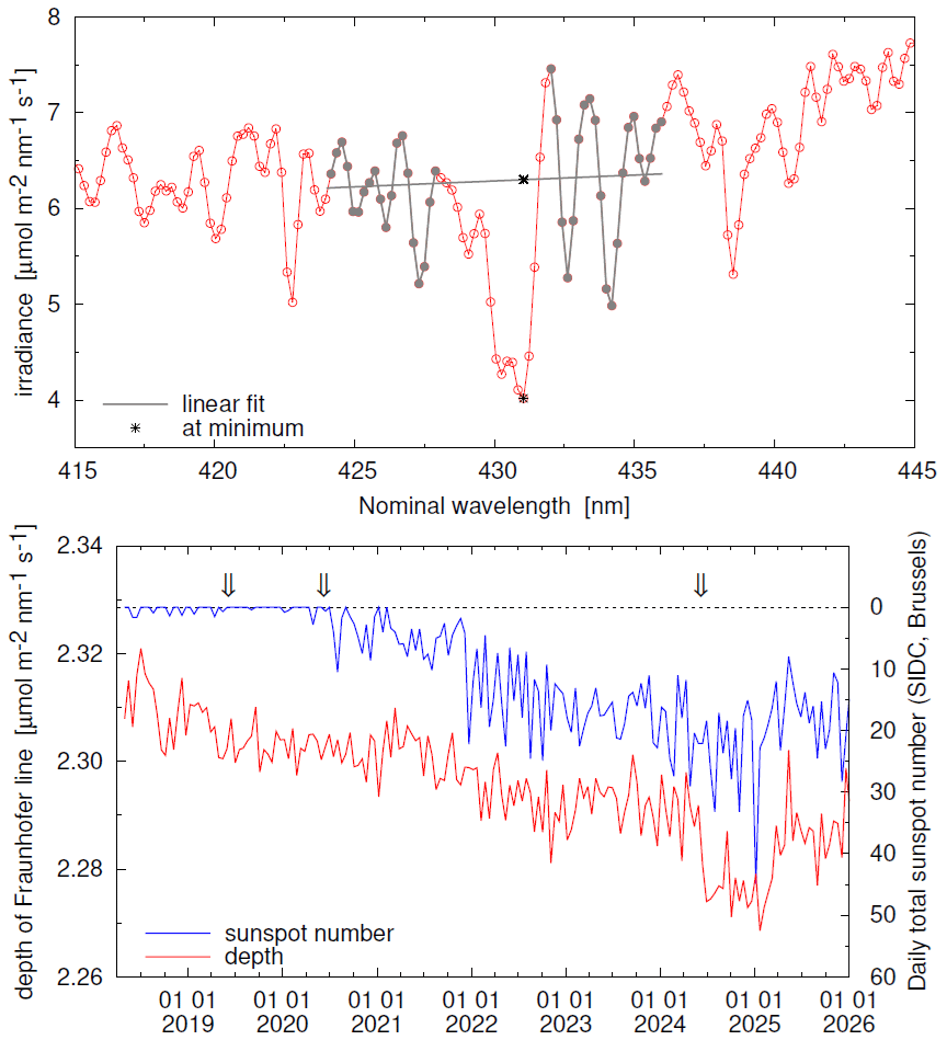
Figure A1 Top panel: definition of the depth of the Fraunhofer line structure around 430 nm using the TROPOMI irradiance of orbit 08518 of 5 June 2019. Bottom panel: change over time of that depth for selected irradiance measurements (red line, left axis) and the daily sunspot number for the same days (blue line, right axis). The arrows at the top point to the dates used in Sects. 3.4 and 4.2. Further details are given in the text of App. A. Source of the sunspot number data: WDC-SILSO, Royal Observatory of Belgium, Brussels.

The evolution over time of this depth is shown in red (left axis) in the bottom panel of Fig. A1, derived from TROPOMI irradiance measurements every 225-th orbit (about once every 15 days), starting with orbit 02818 of 30 April 2018 (the first publicly available TROPOMI irradiance), along with the solar activity in terms of the sunspot number (blue line, right axis, increasing downward): the higher the sunspot number, i.e. the more active the Sun, the less deep is the 430 nm structure. The depth of the two Ca+ Fraunhofer lines near 395 nm (involved in effects of VRS; cf. Sect. 1) vary in a similar way with solar activity (not shown).

Appendix B: Indices of example ground pixels

Table B1 Scanline and row number of Atlantic Ocean (“atl”) and Western Australia (“aus”) ground pixels used in the examples of 5 June 2019; orbit numbers are given between parenthesis in the header line.

Table B2 As Table B1 but for the lake pixel used in Sect. 6.1.

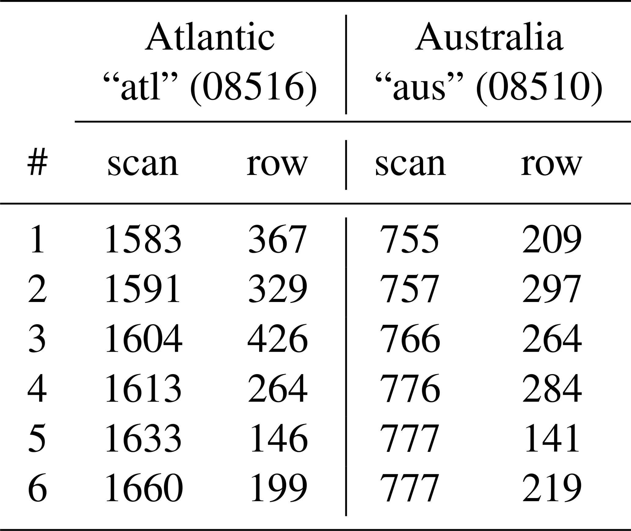
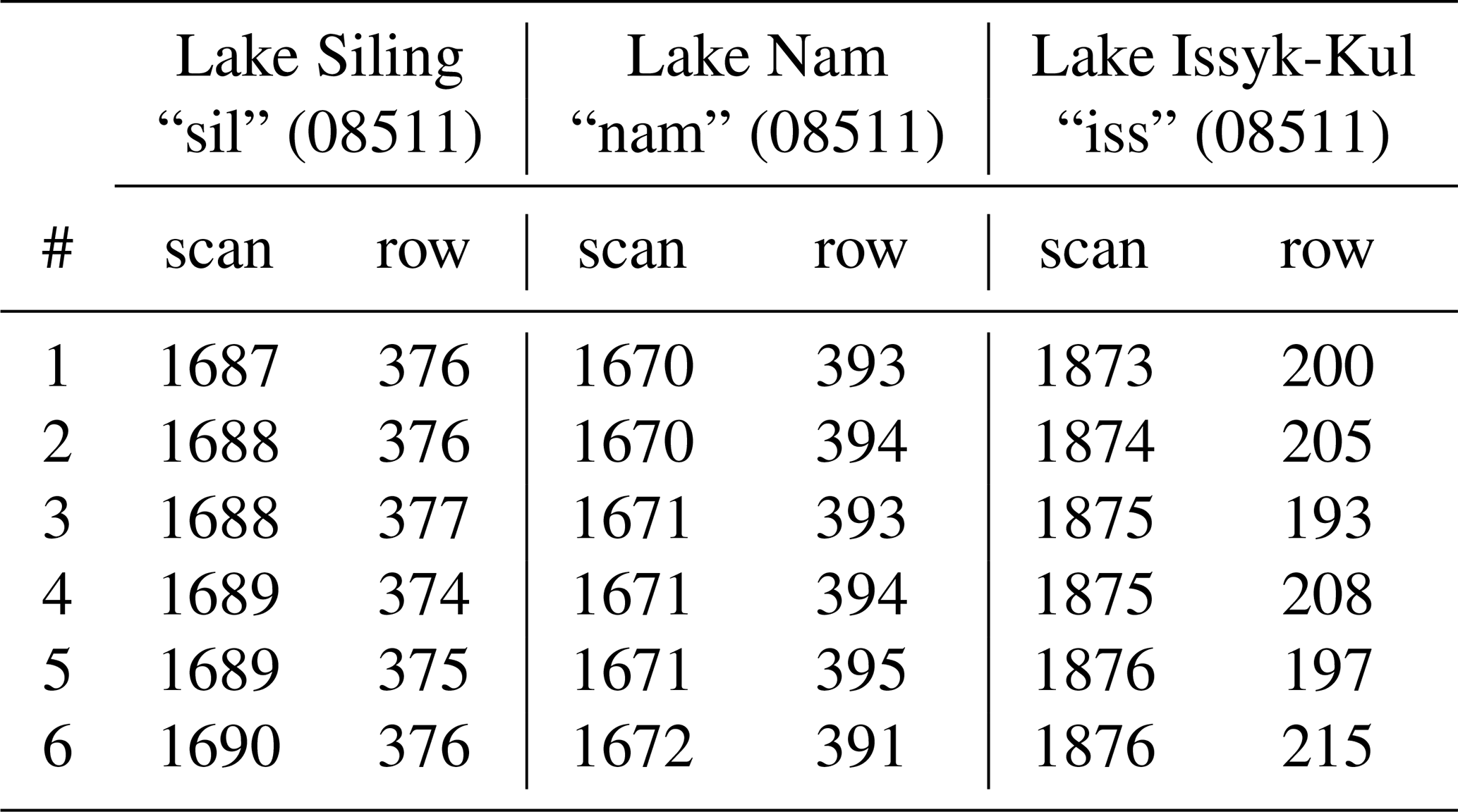
Tables B1 and B2 provide a list of the scanline and row numbers of the example ground pixels used in this paper, labelled by a three-letter identifier.

Appendix C: Additional figures

Figure C1 Colour scale version of Fig. 6 for clear-sky (top) and cloudy (bottom) pixels.

Figure C1 shows a colour scale version of Fig. 6 for clear-sky and cloudy pixels separately.