Satellite-based estimation of high-altitude ice cloud radiative forcing derived through a Rapid Contrail-RF Estimation Approach

Contrails, anthropogenic ice clouds formed by aircraft at cruise altitudes, strongly influence the Earth’s radiation budget but the measurement of their radiative forcing (RF) remains poorly quantified at high temporal resolution. In this study, we present the Rapid Contrail-RF Estimation Approach, which uses geostationary satellite observations to estimate the radiative forcing of high-altitude ice clouds, including potential contrail cirrus clouds. Starting from a cloud retrieval product, we apply pre-computed Look-Up Tables (LUTs) to generate radiative forcing maps for high-altitude ice clouds. Specifically, observations from the Spinning Enhanced Visible and InfraRed Imager (SEVIRI) onboard Meteosat Second Generation (MSG) were used to visually identify days with potential contrails. For 6 selected days, ice clouds were characterized using the Optimal Cloud Analysis (OCA) product from MSG/SEVIRI data provided by the European Organization for the Exploitation of Meteorological Satellites (EUMETSAT). The LUTs were constructed using the libRadtran radiative transfer model to quantify the radiative effect of ice clouds in the short-wave (SW) and long-wave (LW) spectral regions. A cloud top pressure filter was applied to isolate high-altitude ice clouds, including potential contrails. The resulting data set provides a quantification of SW, LW, and net radiative forcing at the top of the atmosphere due to potential contrails. We show that these clouds contribute to daytime cooling and nighttime warming, with a net effect that varies between diurnal cycles. We assess the validity of the Rapid Contrail-RF Estimation Approach through correlation exercises focusing on uncertainties in the use of LUTs, a single ice cloud parameterization, and a calculated cloud top height, supplemented by comparisons with polar orbiting satellite observations from the Clouds and the Earth's Radiant Energy System (CERES) instruments. In general, these correlative comparisons indicate that the proposed approach provides accurate data on the estimation of the radiative forcing of high-altitude ice clouds, including potential contrails, with an accuracy of approximately 15 %.

1 Introduction

Understanding the role of clouds in the Earth’s radiation budget is crucial for mitigating climate change (Wielicki et al., 1995). The IPCC Sixth Assessment Report (IPCC, 2023) highlights that clouds and aerosols still represent the largest source of uncertainty to estimates and interpretations of the Earth's energy budget, particularly when these clouds are caused by anthropogenic activities such as aviation. Aviation contributes approximately 5 % to the anthropogenic climate forcing with the emission of carbon dioxide (CO₂) and non-CO₂ pollutants being the two main contributors (Lee et al., 2009, 2021). The first effects to be clearly identified and linked to the observed global warming were those of CO₂ emissions (Letcher, 2020), which is why many studies and reports initially focused on the quantification of aviation's contribution to the global atmospheric CO₂ concentrations (Olsthoorn, 2001; Pejovic et al., 2008; Ji-Cheng and Yu-Qing, 2012; Mayor and Tol, 2010; Howitt et al., 2011). The delayed onset on research of the non-CO₂ effects is not due to their insignificance for the climate, but rather because these effects are not yet fully understood and remain associated with considerable uncertainty (Lee et al., 2021).

The non-CO₂ aviation effects include emissions of pollutants such as nitrogen oxides (NO_x = NO + NO₂), water vapor (H₂O), soot, sulfur oxides (SO_x) as well as the formation of contrail cirrus clouds (Lee et al., 2021). Among these, contrail cirrus most likely have the largest impact on the TOA radiation budget (Burkhardt and Kärcher, 2011; Brasseur et al., 2016). These aviation-induced clouds are formed behind aircraft cruising in sufficiently cold air due to the emission of water vapor. If the ambient air is sufficiently humid (that is, the relative humidity with respect to ice exceeds 100 %), the contrails can persist, as the ice particles within the contrails grow by deposition of water vapor molecules from the ambient air (Schumann, 2005). When newly formed contrails persist and spread into larger clouds, they are called persistent contrails. This occurs when they are formed in ice supersaturated regions (ISSRs) (Schumann et al., 2017; Unterstrasser, 2020). The properties of the initial contrails, together with their geometric depth and total ice crystal number, will affect the properties of the resulting contrail cirrus clouds (Unterstrasser, 2016). The term contrail cirrus is used for the evolution stage of a contrail when it disperses and loses its line-shaped structure. When we use the term contrail on its own, it corresponds to the combination of persistent contrails and contrail cirrus. Only 10 %–15 % of contrails evolve into contrail cirrus, with an average lifetime of approximately 4 h (Gierens and Vázquez-Navarro, 2018).

The impact of persistent contrails and contrail cirrus on the TOA radiation budget is often quantified using the radiative forcing (RF) (Chen et al., 2000) or the effective RF (ERF) metric. In our case, RF is defined as the radiative impact of a cloud, calculated as the difference in radiative fluxes at TOA between a cloudy and cloud-free atmosphere. ERF, in contrast, includes all tropospheric and land surface adjustments, whereas RF only includes the adjustment due to stratospheric temperature change (Smith et al., 2020). Under most conditions, in the solar wavelength range (i.e., shortwave/SW), persistent contrails and contrail cirrus reflect incoming sunlight back to space, resulting in a negative radiative effect and thus a cooling influence. In the thermal-infrared wavelength range (i.e. longwave/LW), they trap outgoing LW radiation within the Earth-atmosphere system, leading to a positive radiative forcing of LW and an associated warming effect (Heintzenberg and Charlson, 2009). By adding both radiative components, the net radiative effect of the cirrus clouds and consequently, contrails, can be calculated. This net effect can be either positive or negative, depending on the microphysical, macrophysical and optical properties of the contrail cirrus, as well as the radiative properties of the environment (Wolf et al., 2023). For example, cloud properties such as the cloud optical thickness, cloud temperature, and ice crystal shape influence the net radiative response (Kärcher and Burkhardt, 2013; Stephens et al., 2004; Markowicz and Witek, 2011), while environmental parameters like the surface albedo and surface temperature can play a significant role (Schumann and Mayer, 2017).

The estimation of contrails' RF and/or ERF both globally and regionally over extensive time periods is crucial for understanding aviation's contribution to climate change. On a global scale, either general circulation models of the atmosphere, reanalyses data in combination with radiative transfer modeling, or a combination of a model and observations are used to estimate the global yearly mean contrails' net RF and/or ERF (Rädel and Shine, 2008; Lee et al., 2021; Gettelman et al., 2021; Bock and Burkhardt, 2016; Chen and Gettelman, 2013; Bier and Burkhardt, 2022; Teoh et al., 2024). These studies have reported that the presence of contrails has a yearly positive global net radiative impact, which varies significantly among studies, ranging from 6 mW m⁻² (Rädel and Shine, 2008) to 62.1 mW m⁻² (Teoh et al., 2024). On smaller spatial and temporal scales, studies have been carried out using polar-orbiting satellite observations, geostationary ones or a combination of both (Haywood et al., 2009; Wang et al., 2024; Dekoutsidis et al., 2023; Duda et al., 2004; Mannstein and Schumann, 2005; Graf et al., 2012; Schumann and Graf, 2013; Wang et al., 2023; Meijer et al., 2022). The development of efficient and convenient methods for the observation of RF from contrails is thus necessary to extend the spatial and temporal coverage of their radiative impact studies.

Once the contrails are detected, radiative transfer models can be used to quantify their radiative effect at the TOA. Although it is not the only way to perform such a task (Haywood et al., 2009), radiative transfer models are a useful tool to quantify the radiative impact of clouds. In the study of Wang et al. (2024), the quantification of the net effect of contrail cirrus is conducted by performing full radiative transfer calculations with the inputs being the measured cloud and environmental properties for each satellite pixel over Western Europe for 2 d. It has been proposed by Wolf et al. (2023) that once the cloud and environmental properties are well-described, a large number of RT simulations can be performed ahead of time to construct ice clouds RF LUTs instead of performing the full radiative transfer calculations for each pixel. By using visible and infrared imagers aboard geostationary satellites, the observation capability of contrails is limited in terms of cloud optical depth (COD). In Driver et al. (2025), the authors remark on the basis of simulated contrail detection that there is a lower bound of about 0.05 in COD (thinner contrails are not detected). This limitation applies to the detection of contrails but implies that the RF estimates can only be performed on the detected clouds, which misses part of the contrail lifecycle.

The use of RF LUTs combined with geostationary satellite observations offers many advantages but also presents some drawbacks. By performing a large number of radiative transfer simulations once, while varying relevant parameters, such as the solar zenith angle, the surface albedo, the ice cloud's optical thickness, etc., we can construct multi-dimensional LUTs, which describe the behavior of the solar and thermal/infrared RF (RF_sol and RF_tir, respectively) as a function of these parameters. Then, these LUTs can be merged with geostationary satellite observations to generate contrails RF maps. Large datasets can be processed relatively quickly, enabling the analysis of full years of geostationary data and the study of daily and seasonal patterns of contrails RF. Furthermore, once the LUTs are constructed, they are independent of the satellite instrument's characteristics, allowing them to be merged with different satellite observations. However, the primary concern with using LUTs is how accurately they represent the real atmospheric conditions for each pixel. Often, LUTs are built using standard atmospheric profiles or specific ice cloud properties, which may not capture the variability of real atmospheric conditions.

In this study, we present a new satellite-based approach for generating RF maps of high-altitude ice clouds. We refer to this new approach as Rapid Contrail-RF Estimation Approach, as it is applied to high-altitude ice clouds, including potential contrails. A methodological flowchart of the approach is presented in Fig. 1. The Rapid Contrail-RF Estimation Approach combines geostationary satellite observations, a cloud properties retrieval algorithm and radiative transfer modeling. In the present work, we use a cloud top pressure filter to select high-altitude ice clouds, including potential contrails. This methodology is not sufficient to discriminate contrails but allows us to validate our RF estimation on ice clouds in general. We discuss the relevance of this limitation and future directions in our conclusions.

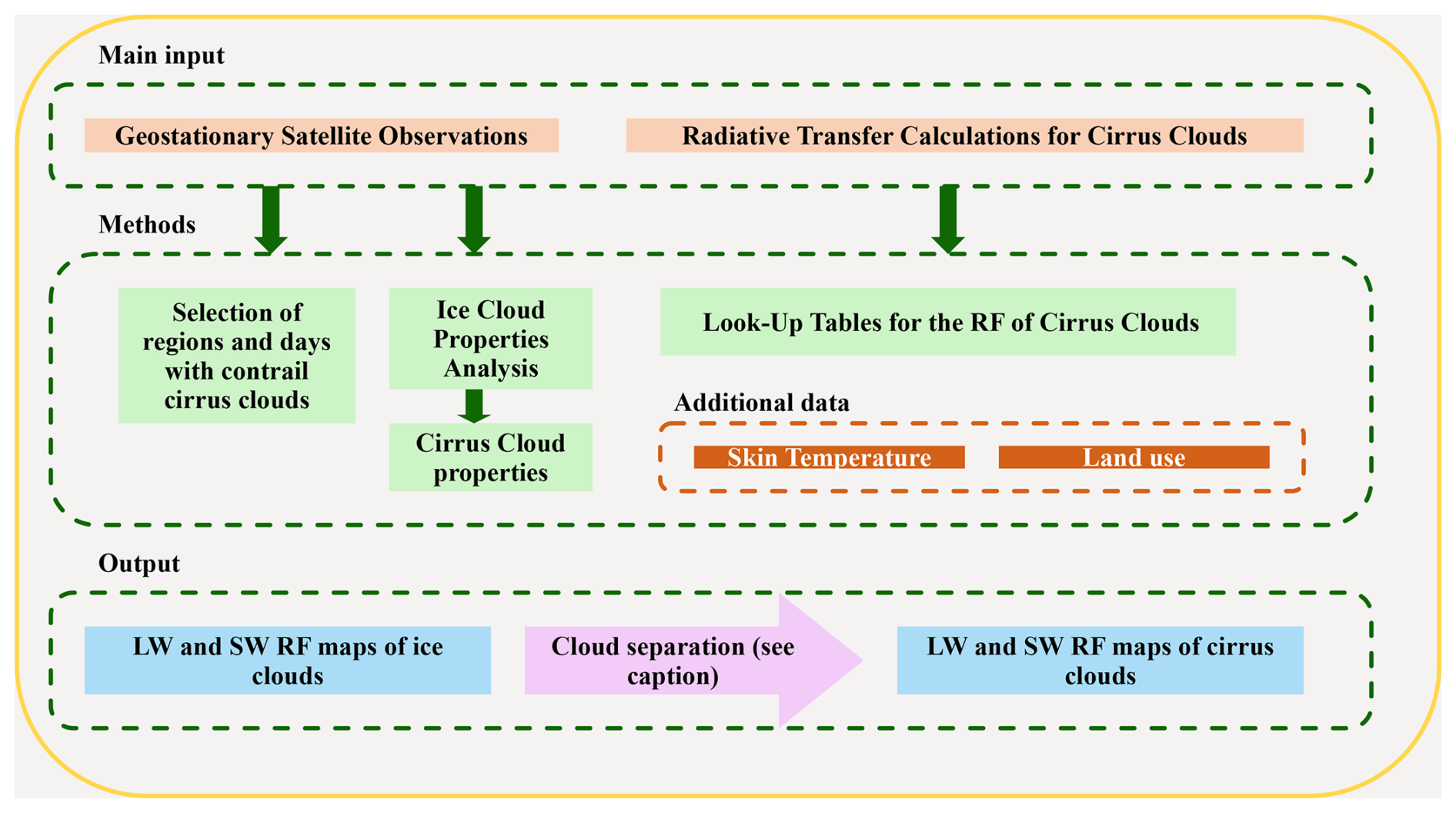
Figure 1 Methodological flowchart describing the Rapid Contrail-RF Estimation Approach. In the present study, the cloud separation scheme is based on a simplified cloud top pressure filter (see Sect. 3.2).

First, MSG/SEVIRI observations were employed to visually identify days with the presence of potential contrails. For the selected days, the detection and characterization of ice clouds, including those overlapping with lower-layer clouds, were performed using the OCA product (EUMETSAT, 2016) derived from MSG/SEVIRI data. Second, LUTs were constructed using the libRadtran RT model (Emde et al., 2016) to quantify the radiative effects of thin to semi-transparent ice clouds in both the SW (reflected solar radiation) and LW (thermal radiation) spectral regions. Third, the retrieved cloud properties were combined with the LUTs to generate radiative forcing maps of natural cirrus, persistent contrails, and contrail cirrus clouds, with a 15 min temporal resolution on a regular grid of spatial resolution equal to 0.04°. Finally, a cloud top pressure separation scheme is used as a substitute for potential contrail detection. The dataset covers 6 different days within the 2023–2024 period on a geographic area expanding from 30° W to 15° E longitude and 25 to 55° N of latitude. We used the generated RF maps of potential contrails to investigate their behavior with respect to the TOA radiation budget. The uncertainty of the Rapid Contrail-RF Estimation Approach has been assessed via three different validation exercises by evaluating (1) the choice of using a single atmospheric vertical profile in the RT simulations, (2) the choice of a single ice cloud parameterization scheme, and (3) the impact of using CTH values estimated by a single atmospheric vertical profile on the RF estimations. Additionally, an end-to-end validation is performed by comparing the flux maps for potential contrail cirrus and polar-orbiting satellite observations from the CERES instruments. A comparison between our results and those reported in Wang et al. (2024) for two contrail cirrus outbreaks is also presented.

The paper is organized into five sections. Section 2 contains the Rapid Contrail-RF Estimation Approach for generating RF maps for potential contrail cirrus clouds, followed by the necessary data. In Sect. 3 a description of the methodology for merging the different datasets is provided. The main results of the study, along with five different validation exercises to assess the validity and estimate the uncertainty of the Rapid Contrail-RF Estimation Approach, are discussed in Sect. 4. A detailed validation of the Rapid Contrail-RF Estimation Approach is provided in Sect. 5. Finally, conclusions and future perspectives are discussed in Sect. 6.

2 Data for the Rapid Contrail-RF Estimation Approach

In this study, the Rapid Contrail-RF Estimation Approach is deployed to generate RF maps for high-altitude ice clouds above the geographic area of interest, following these three initial steps: (1) detection (Sect. 2.1), (2) characterization (Sect. 2.2), and (3) estimation of the RF (Sect. 2.3) for high-altitude ice-clouds.

Additionally, different datasets have been employed for two main purposes: (1) to accurately describe the conditions and characteristics of the geographic area of interest (see Sect. 2.4 and 2.5) and (2) to validate the RF maps of high-altitude ice-clouds (see Sect. 2.4 and 2.6). A flowchart describing the Rapid Contrail-RF Estimation Approach is presented in Fig. 1.

2.1 Geostationary Satellite Observations

The detection and characterization of ice clouds was carried out using data from the SEVIRI on board MSG-3 (Meteosat-10) satellite, which is operated by EUMETSAT. MSG-3 is located at 0° longitude in geostationary orbit, approximately 36 000 km above the Earth's surface (Schumann et al., 2002). SEVIRI provides spectral information across 11 spectral channels, with a temporal resolution of 15 min and a spatial resolution of approximately 3 × 3 km² at the sub-satellite point (SSP) (Roberto, 2010; Huckle and Fischer, 2009).

Our primary objective is to investigate the behavior of potential contrails above different surface types, and times of the day. These clouds can be visually detected using the Dust/RGB (Red, Green, Blue) composite, which combines data from the MSG/SEVIRI IR8.7, IR10.8 and IR12.0 channels. In this product, the contrails appear as long bluish and reddish lines and are visually distinguished to other cloud types (see Fig. 7). Previous studies such as Wang et al. (2023), Schmetz et al. (2002), and Dekoutsidis (2019), also successfully utilized the Dust/RGB composite to detect contrails. In this study, using this composite, with the aid of the Satpy Python library (Hoese, 2019) and the EUMETSAT RGB recipes (https://eumetrain.org/manualguides/rgb-recipes, last access: 15 April 2025)), we identified specific days during which we could visually detect geographic regions above Europe and parts of the North Atlantic Ocean where persistent contrails were present.

In summary, the study area extends from 30° W to 15° E of longitude and 25 to 55° N of latitude covering data from 6 different days: 30 January 2023; 13 June 2023; 25 September 2023; 30 January 2024; 17 February 2024; and 28 May 2024. The geostationary grid has been re-projected onto a regular grid with a spatial resolution of 0.04°.

2.2 Cloud Analysis Product

In the present study, the OCA product is used for the physical characterization of the detected ice clouds.

The OCA algorithm uses the Optimal Estimation (OE) method along with spectral measurements simultaneously to retrieve the cloud state parameters (Rodgers, 2000; Mecikalski et al., 2011; EUMETSAT, 2016).

The OCA product is available at a 15 min frequency and at the full earth scanning area in GRIB format (EUMETSAT, 2019a). It contains single-layer as well as multi-layer cloud situations and the product is structured in layers numbered in a top-down notation: the first layer (named Layer-One) is the highest layer (closest to the top of the atmosphere) and the second layer (named Layer-Two) is the lower layer, which only exists when the pixel has multi-layer cloud conditions (Watts et al., 2011). It should be noted that for the multi-layer cloud scenes, the upper layer is assumed to be an ice cloud and the lower layer a liquid water cloud.

For the present study, we will focus only on pixels characterized as ice or multi-layered clouds (cloud phase) and will use both COT and CTP for the two layers and CER only for the ice cloud. An additional parameter is CTH, which is not included in the OCA product. As we are using a US Standard atmosphere for the construction of the LUTs (see Sect. 2.3), the same profile has been used to linearly interpolate CTP in the pressure vertical grid, and consequently the altitude vertical grid, of the US Standard atmosphere (Anderson et al., 1986). The uncertainty related to the use of a calculated CTH is presented in Sect. 5.3.

2.3 Radiative Transfer Calculations

LUTs of thin to semi-transparent high-altitude ice clouds are constructed using the libRadtran software (Emde et al., 2016). Apart for the range of the parameters, which should be verified by users of these tables, the method here is applicable to naturally occurring cirrus clouds as well as to contrails. In this work, we perform the validation on all ice clouds that are selected by a cloud top pressure filter.

The libRadtran RT library (version 2.0.5) is used to construct LUTs of TOA irradiances for the SW (reflected solar radiation) and LW (emitted thermal radiation) spectral regions, separately. The RT simulations were performed with the one-dimensional (1-D) DIScrete ORdinate Radiative Transfer (DISORT) solver (Stamnes et al., 2000), which is included in the libRadtran software package. Using a 1-D solver means that the ice clouds are assumed to be horizontally uniform.

The spectra for both the SW and LW wavelength regions are simulated under three different scene scenarios:

1. Ice cloud above ocean surface,

2. Ice cloud above land surfaces, and

3. Ice cloud above a liquid water cloud.

and, the following input parameters are chosen:

• 16 streams to solve the RT equation, which provides accurate results and limits the computational time.

• a US-standard atmosphere as the main atmospheric profile. The accuracy of such a simplification is assessed in Sect. 5.1.

• the ice crystal shape to be moderately rough aggregates of eight-element columns based on the ice cloud parameterization of Yang et al. (2013). The uncertainty related to the use of a single ice crystal shape scheme is discussed in Sect. 5.2.

• the ice water content and effective particle radius to be translated to optical properties based on the ice cloud parameterization of Yang et al. (2013).

• the built-in International Geosphere Biosphere Programme (IGBP) library which is a collection of spectral albedos of different surface types.

• the liquid water content and effective radius of the liquid water cloud to be translated to optical properties based on the parameterization of Hu and Stamnes (1993).

In the SW spectral region, the spectra are simulated from 250 up to 5000 nm, while in the LW wavelength region, from 2500 up to 98 000 nm.

For the LW spectral region and an ice cloud above land and ocean surfaces, the molecular absorption is considered by using the fine resolution REPTRAN parameterization from Gasteiger et al. (2014). For an ice cloud above a liquid water cloud, the same molecular absorption is used but at medium resolution.

Six examples of libRadtran input files (i.e., one in the SW and one in the LW for the three scene scenarios) are provided on the Zenodo platform at https://doi.org/10.5281/zenodo.14859250 (de Buyl, 2025).

The initial output files of the RT simulations in the SW and LW spectral regions contain the wavelength, the output altitude, the direct beam irradiance with respect to the horizontal plane, the diffuse down irradiance and the diffuse up irradiance. These variables are integrated over the total simulation wavelength range separately in the SW and LW wavelength regions to estimate the TOA downward and upward solar/thermal-infrared irradiances (F_down and F_up, respectively).

RF_sol and RF_tir of ice clouds are defined as the difference in fluxes between the ice cloud (F_ic) and ice cloud-free (F_icf) atmosphere at the TOA:

$$\begin{array}{}\text{(1)}& \text{RF}=F_{\mathrm{ic}}-F_{\mathrm{icf}}={\left[F_{\mathrm{down}}-F_{\mathrm{up}}\right]}_{\mathrm{ic}}-{\left[F_{\mathrm{down}}-F_{\mathrm{up}}\right]}_{\mathrm{icf}}\end{array}$$

Then, the net RF is a summation between RF_sol and RF_tir (Wolf et al., 2023). It should be noted that negative RF values indicate cooling, while positive ones correspond to warming.

In the SW wavelength range, the LUTs store the TOA F_down, F_up, and RF_sol as a function of the following parameters:

• the Solar Zenith Angle (SZA), COT and CER for an ice cloud above ocean surface,

• the SZA, COT, CER and underlying surface type as defined by the IGBP for an ice cloud above land surface, and

• the SZA, COT, CER and liquid water Cloud Optical Thickness (wCOT) for an ice above a liquid water cloud.

while keeping the following constant:

• the CTH equal to 10 km for the three scene scenarios,

• the ocean Bidirectional Reflectance Distribution Function (BRDF) determined by a wind speed equal to 5 m s⁻¹ for an ice cloud above ocean surface from Cox and Munk (1954a, b),

• the water Cloud Top Height (wCTH) equal to 3 km for an ice cloud above a liquid water cloud.

The LUTs in the LW store the TOA F_down, F_up, and RF_tir by varying the following parameters:

• the SST, CTH, COT, and CER for an ice cloud above ocean surface,

• the underlying LST, CTH, COT, CER and IGBP surface type for an ice cloud above land surface,

• the wCOT, wCTH, CTH, COT, and CER for an ice cloud above a liquid water cloud.

To save computational time, RT simulations have been performed for all IGBP surface types in the SW spectrum but not in the LW spectrum. In the SW spectrum, there are 17 different LUTs, each corresponding to simulations for the 17 different IGBP surface types. The only IGBP surface type not included in these simulations is type 17 (ocean water). For this type, the LUTs correspond to the scenario of an ice cloud above an ocean surface. In the LW, RT simulations were conducted for 8 specific IGBP surface types (i.e., evergreen needle forest, closed shrubs, open shrubs, woody savanna, grassland, urban, antarctic snow, and desert). The other IGBP surface types were mapped to the existing ones based on their similar or closely related emissivity responses.

The LUTs are all stored in a single NetCDF file and are available on the Zenodo platform at https://doi.org/10.5281/zenodo.14859250 (de Buyl, 2025).

The reader should note that the RF values stored in the different LUTs depend on at least three parameters (e.g., SW wavelength range and the scene scenario of ice cloud above ocean) and up to five parameters (e.g., LW wavelength range and the scene scenario of ice cloud above a liquid water cloud). It is complex to illustrate every single dependency of RF with respect to each input parameter. Therefore, we have chosen to demonstrate some of these dependencies in Figs. 2 and 3.

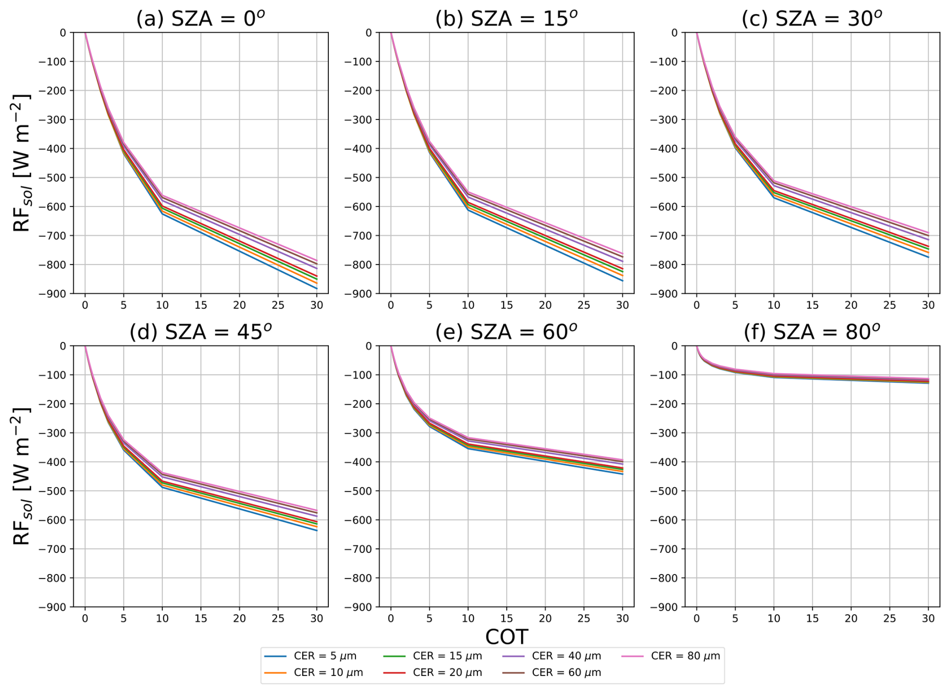
Figure 2 Radiative forcing (RF) in the shortwave (SW) wavelength range (RF_sol) as a function of the cloud optical thickness (COT) for different values of ice crystal effective radius (CER) for an ice cloud over the ocean presented for six different solar zenith angle (SZA) values ranging from (a) 0° to (b) 80°.

Figure 2 presents an example of the variation of RF_sol for an ice cloud above ocean as a function of COT, SZA (different plots), and CER (different lines in every plot). In the SW wavelength range, RF is negative, corresponding to a cooling effect of the climate at the TOA due to cloud reflectivity. As observed, RF_sol increases in magnitude as the ice cloud becomes optically thicker (larger COT values). Additionally, the size of the ice crystals (i.e., CER) becomes significant for optically thick clouds. Finally, as we can see, the SZA also plays an important role in the simulations, resulting in larger absolute RF_sol values for a SZA value equal to 0°.

Similar to Fig. 2, Fig. 3 demonstrates the variation of RF_tir for an ice cloud above the ocean as a function of COT, SST (different plots), and CER (different lines in every plot). Here, we observe that RF_tir changes rapidly for small values of COT, specifically in the range from 0 to 10. However, RF_tir saturates when the cloud reaches a certain optical thickness (approximately a COT equal to 10). The influence of SST on the RF increases as the cloud becomes optically thicker. Additionally, when SST and COT increases, and consequently the infra-red radiation is trapped between surface and ice cloud, RF_tir becomes larger. Finally, CER does not have as large an effect as it does on RF_tir in the SW wavelength range.

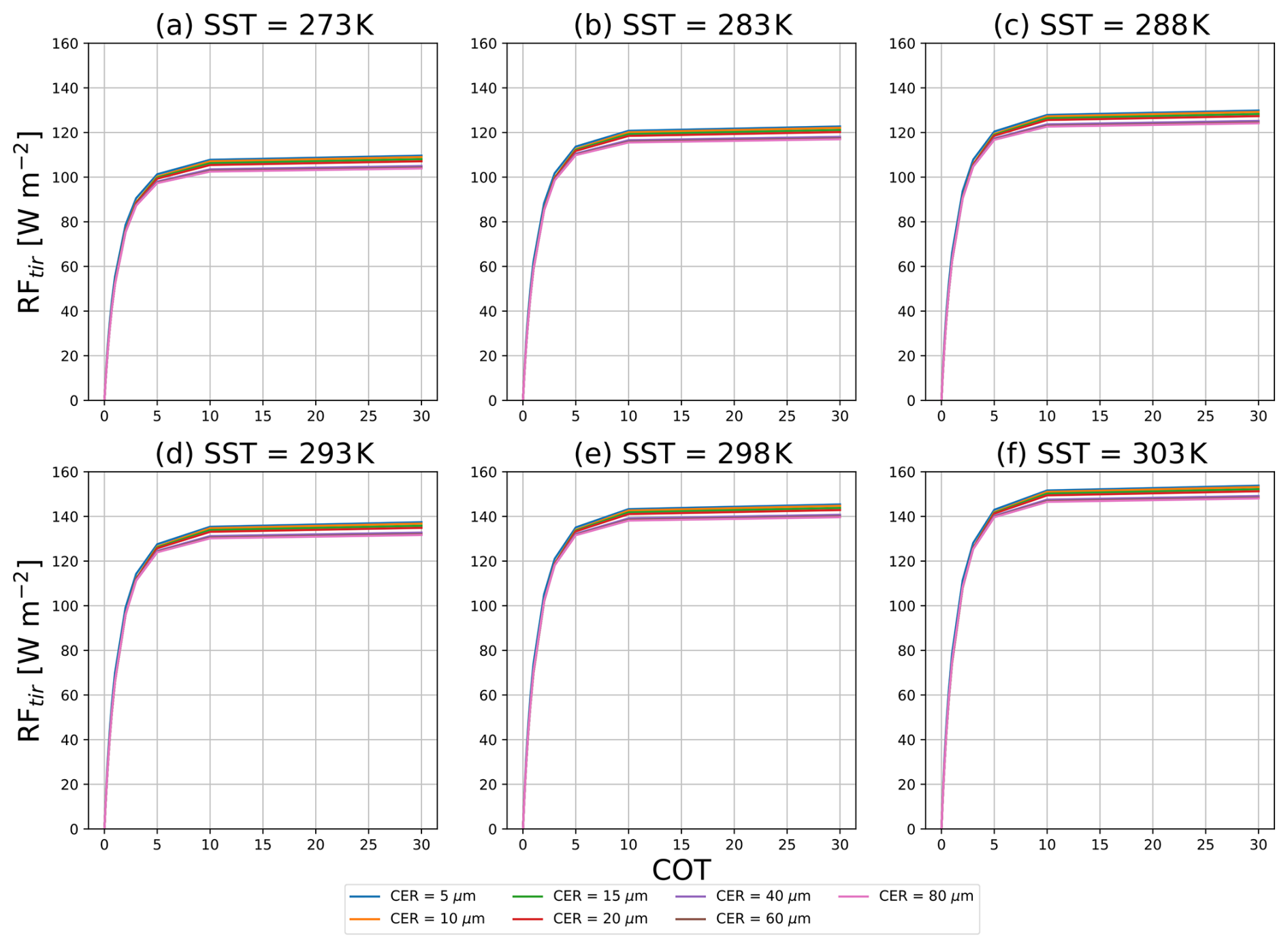
Figure 3 Radiative forcing (RF) in the longwave (LW) wavelength range (RF_tir) as a function of the cloud optical thickness (COT) for different values of ice crystal effective radius (CER) for an ice cloud over the ocean presented for six different sea surface temperature (SST) values ranging from (a) 273 K to (f) 303 K. For visual clarity, the SST value equal to 278 K is not presented here.

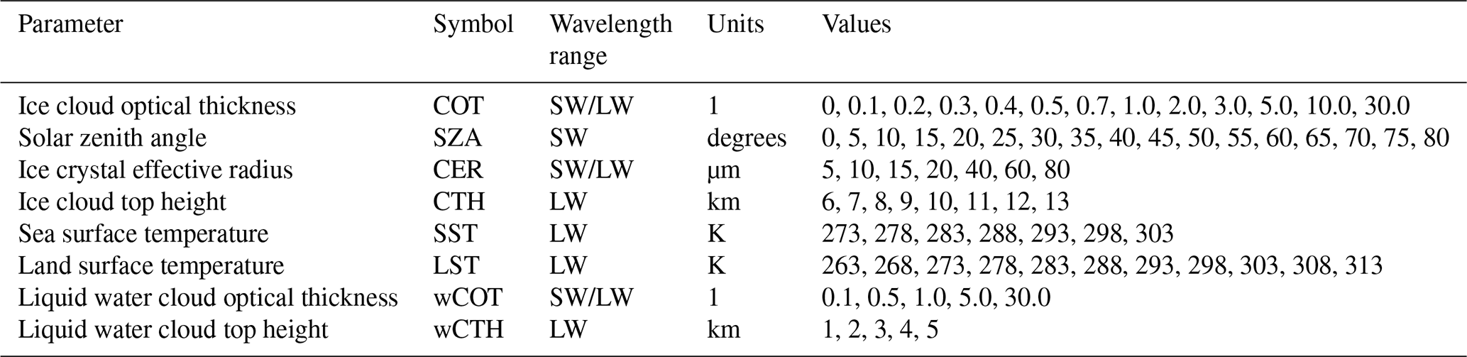
Table 1 provides a summary of all the parameter used in RT simulations with their respective symbol, unit, and range of values.

Table 1 Parameter values used in the SW and LW radiative transfer model (RTM) simulations.

2.4 Surface temperature and vertical temperature profiles

As will be seen in Sect. 3.1, an important input for the LW RT simulations is the surface temperature, called skin temperature (SKT), in the geographic area of interest for each selected day. SKT maps are downloaded from the Meteorological Archival and Retrieval System (MARS) archive for the forecast stream (fc) of the European Center for Medium-Range Weather Forecasts (ECMWF) for the 6 selected days. The data are re-gridded on a regular grid with a spatial resolution equal to 0.04°, covering the geographic domain of this study (see Fig. 4). The data are based on the 00:00:00 and 12:00:00 UTC analysis, each covering the subsequent 12 h forecast period in a time resolution of 1 h. For MSG/SEVIRI observations falling between two time steps, linear interpolation is performed between the two successive time steps to assign SKT maps to those observations.

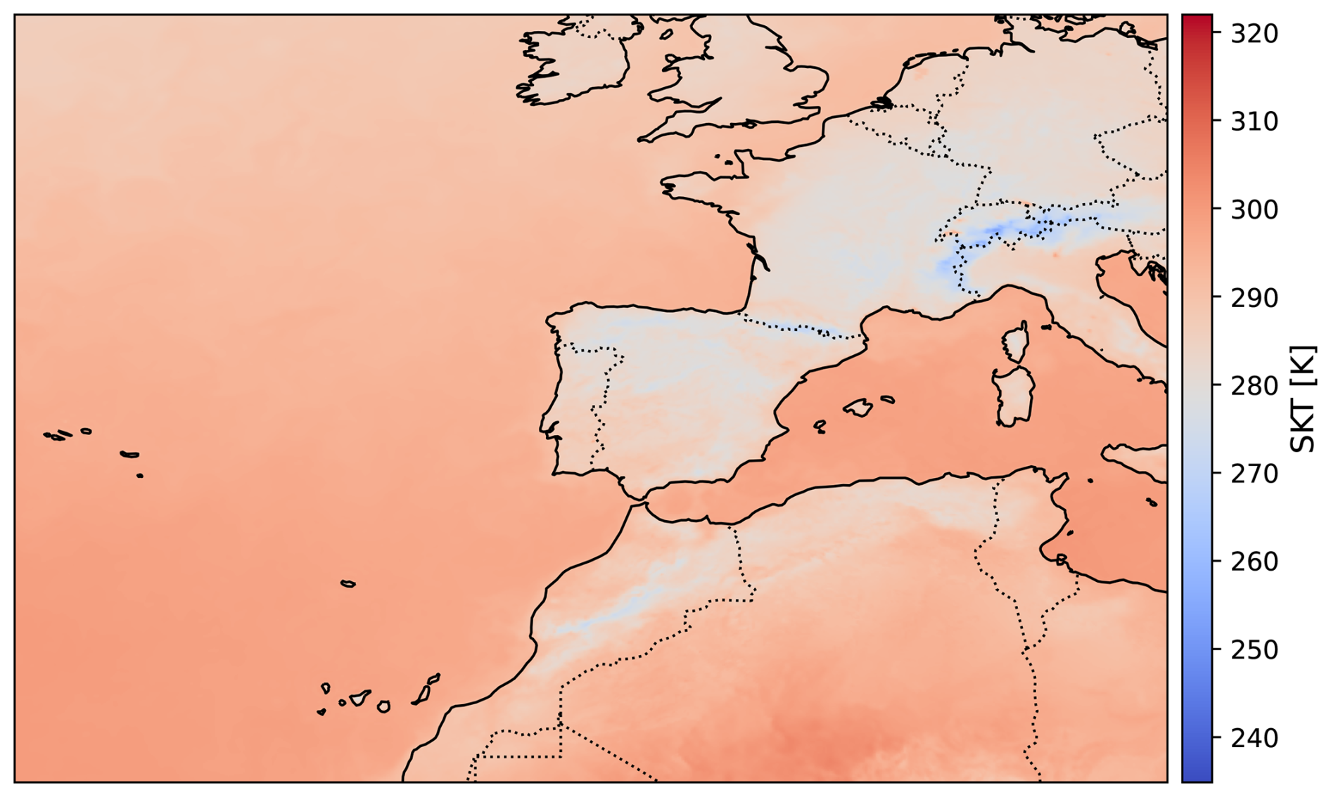
Figure 4 Skin temperature (SKT) map for an example date and observation time (25 September 2023 and 06:00:00 UTC) over the study area.

To assess the validity of using a single atmospheric vertical temperature profile, radiative transfer simulations were performed for selected pixels by using real vertical temperature profiles instead of the LUTs in a number of randomly selected pixels (see Sect. 5.1). For this purpose, we downloaded hourly ERA5 vertical temperature profiles from the ECMWF's MARS archive for the analysis stream re-gridded onto a regular grid with a spatial resolution of 0.04°. The temperature profiles are temporally interpolated into the MSG/SEVIRI observation time by using linear interpolation between the analysis data at the previous and next hour.

2.5 Land use

Using a representative land use dataset for the geographic area of interest is essential because it affects the RT simulations in the LW wavelength range through the surface aldedo and emissivity. We utilize the Terra and Aqua combined Moderate-Resolution Imaging Spectroradiometer (MODIS) Land Cover Type (MCD12Q1) Version 6.1 data for the most recent available year, 2022. The MCD12Q1 data are provided as tiles approximately 1000 × 1000 km² using a sinusoidal grid. The data are re-projected on a regular grid with a spatial resolution of 0.04° in the geographic domain of interest (see Fig. 5) with the aid of Satpy Python library (Hoese, 2019).

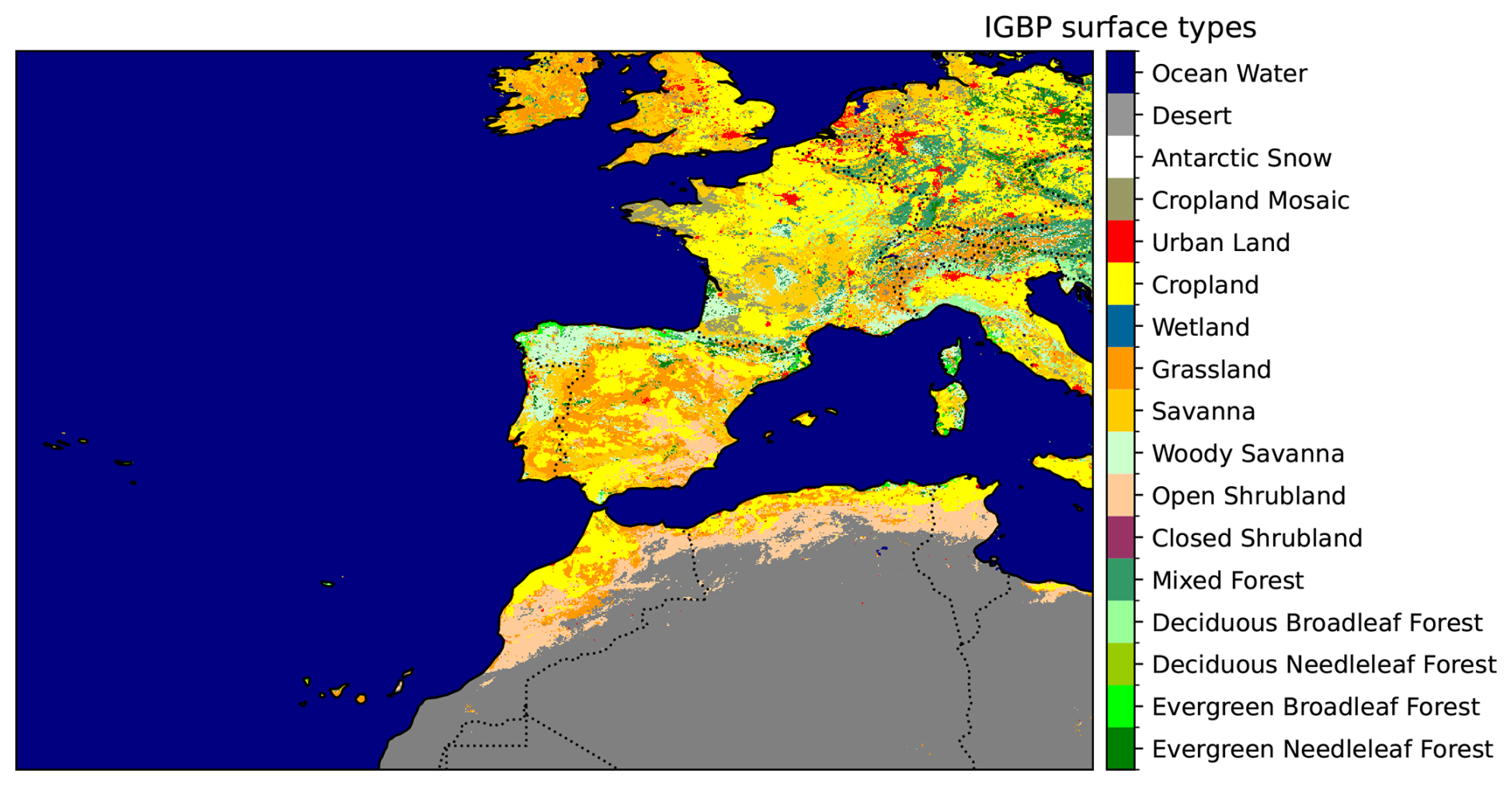
Figure 5 International Geosphere Biosphere Programme (IGBP) land use classification scheme in the selected geographic domain of this study from the MCD12Q1 Version 6.1 data product.

In this study, we employ the IGBP global vegetation classification scheme, which identifies 17 different land cover classes. It should be noted that in the case of pixels being covered by multiple IGBP classes, we assign the land cover value with the largest percentage coverage to that pixel, with a special treatment for water. We first discriminate whether the pixel is covered by water for more than half of its fine-scale MODIS pixels, in which case it is assigned the water class. Else, we consider all non-water classes for the majority choice.

2.6 Polar Orbiting Satellite Observations

The CERES instruments aboard Terra measure the Earths' total radiation budget (Barkstrom, 1999). This type of satellite observations are essential for assessing the radiative effect of clouds.

The Single Scan Footprint (SSF) TOA/Surface Fluxes and Clouds product contains instantaneous CERES observations for a single scanner instrument (NASA Langley Atmospheric Science Data Center, 2019). The data used in this study combine CERES observations with scene and cloud properties from MODIS on Terra and Aqua satellite.

In this study, we use TOA SW and LW fluxes from CERES Terra-Flight Model 1 (FM1) and Aqua FM3 Edition 4A SSF to validate the TOA SW and LW flux maps of high-altitude ice-clouds derived using the Rapid Contrail-RF Estimation Approach (see Sect. 5).

3 Methodology of the Rapid Contrail-RF Estimation Approach

Here, we present the methodology followed, first to merge the three principal datasets introduced in Sect. 2 with the necessary additional data, and finally, to separate potential contrails from natural cirrus clouds (Sect. 3.2).

3.1 Merging the principal datasets

First, as described in Sect. 2.1, we use the MSG/SEVIRI Dust/RGB composite to identify specific days during which persistent contrails could be visually detected. It should be noted that contrails with COT values lower than 0.05 are undetectable when using imaging instruments aboard geostationary satellites (Kärcher et al., 2009; Driver et al., 2025). For these particular days, the OCA product is re-gridded onto a regular grid with a spatial resolution equal to 0.04°, covering the study area, which expands from 30° W to 15° E longitude and 25 to 55° N latitude. The necessary additional data, including SKT data (see Sect. 2.4) and the surface type (see Sect. 2.5), are also resampled onto the same regular grid with the same spatial resolution as the re-gridded OCA product. As a result, the generated maps contain pixels with information on the cloud phase (cloud-free, liquid, ice, or multi-layered clouds), CTP, COT, CER, SKT, and surface type.

For each pixel characterized as an ice or multi-layered cloud, we first determine which LUT should be used among the three scene scenarios by utilizing the surface type information (land or ocean) and the OCA cloud phase (ice or multi-layered). Once the choice of LUT is made, a multi-dimensional interpolation of the simulated RF_sol and RF_tir values from the LUT at the actual values of the cloud and environmental parameters for each pixel (SZA, COT, SKT etc.) is performed.

The dimensions of the interpolation are determined by the number of parameters on which RF_sol and RF_tir depend in each LUT. For instance, for an ice cloud above ocean and within the SW wavelength range, a 3-dimensional interpolation is performed with the simulated RF_sol being a function of COT, CER, and SZA parameters. For the same scene within the LW wavelength range, a 4-dimensional interpolation is necessary, where simulated RF_tir is a function of COT, SST, CTH, and CER parameters.

The final output of this approach is the construction of RF_sol and RF_tir, as well as F_sol and F_tir maps of the detected ice clouds.

3.2 Selection of high-altitude ice clouds

Merging the different datasets, as explained in Sect. 3.1, will generate RF and fluxes maps of both natural and aviation-induced clouds. To emulate the detection of potential persistent contrails, among naturally occurring and contrail clouds, we apply a filtering method based on the ice clouds' CTP value similar to the approach described in Wang et al. (2024). This procedure does not allow for an impact study of aviation but is sufficient to validate our method.

The rationale behind this approach is that most of commercial airplanes fly at altitudes ranging from 8 to 12 km, which corresponds to a mean pressure level of 250 hPa. However, for a persistent contrail or a contrail cirrus to form, specific atmospheric conditions are required, mainly the presence of an ISSR. On average, these ISSRs are typically found at slightly higher pressure levels, around 300 hPa. Combining both information, we implement a CTP filter at 300 hPa in our analysis, meaning that clouds above 300 hPa may contain persistent contrails or contrail cirrus. It should be noted that this approach provides a rough and approximate filtering compared to better approaches, such as manually labeling remote sensing images (Meijer et al., 2022), or contrail detection algorithms based on machine learning (Ortiz et al., 2024).

4 Results

In this section, we first present the main results of the study (Sect. 4.1 and 4.2) including the detection and characterization of potential contrails as well as their RF.

4.1 Detection and characterization of potential contrails

The detection and characterization of potential contrails are conducted for each selected day by zooming on smaller geographic regions within our spatial domain of interest, based on the presence of a large number of potential contrails. This choice significantly reduces the computational time for Sect. 5.1, 5.3, and 5.4, while allowing us to sample pixels over land or ocean on the different days. Figure 6 presents the selected longitude and latitude ranges for each day, while Table 2 provides a summary.

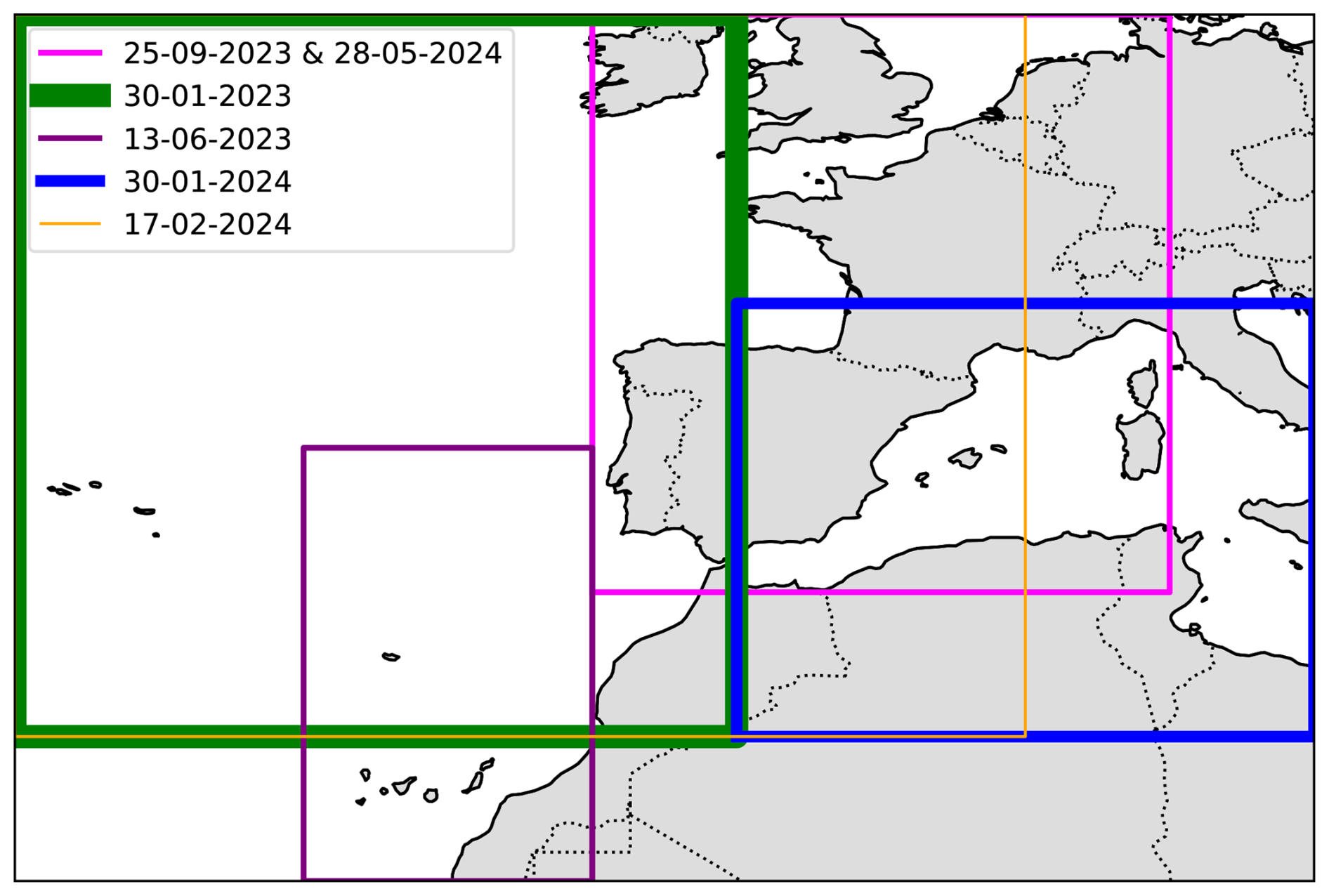
Figure 6 Geographic map of the overall geographic region, illustrating different colored boxes that represent the zoomed geographic areas of interest per day.

Table 2 Selected days, and the geographic limits of each zoomed regions within the geographic area of interest where potential persistent contrails were visually detected.

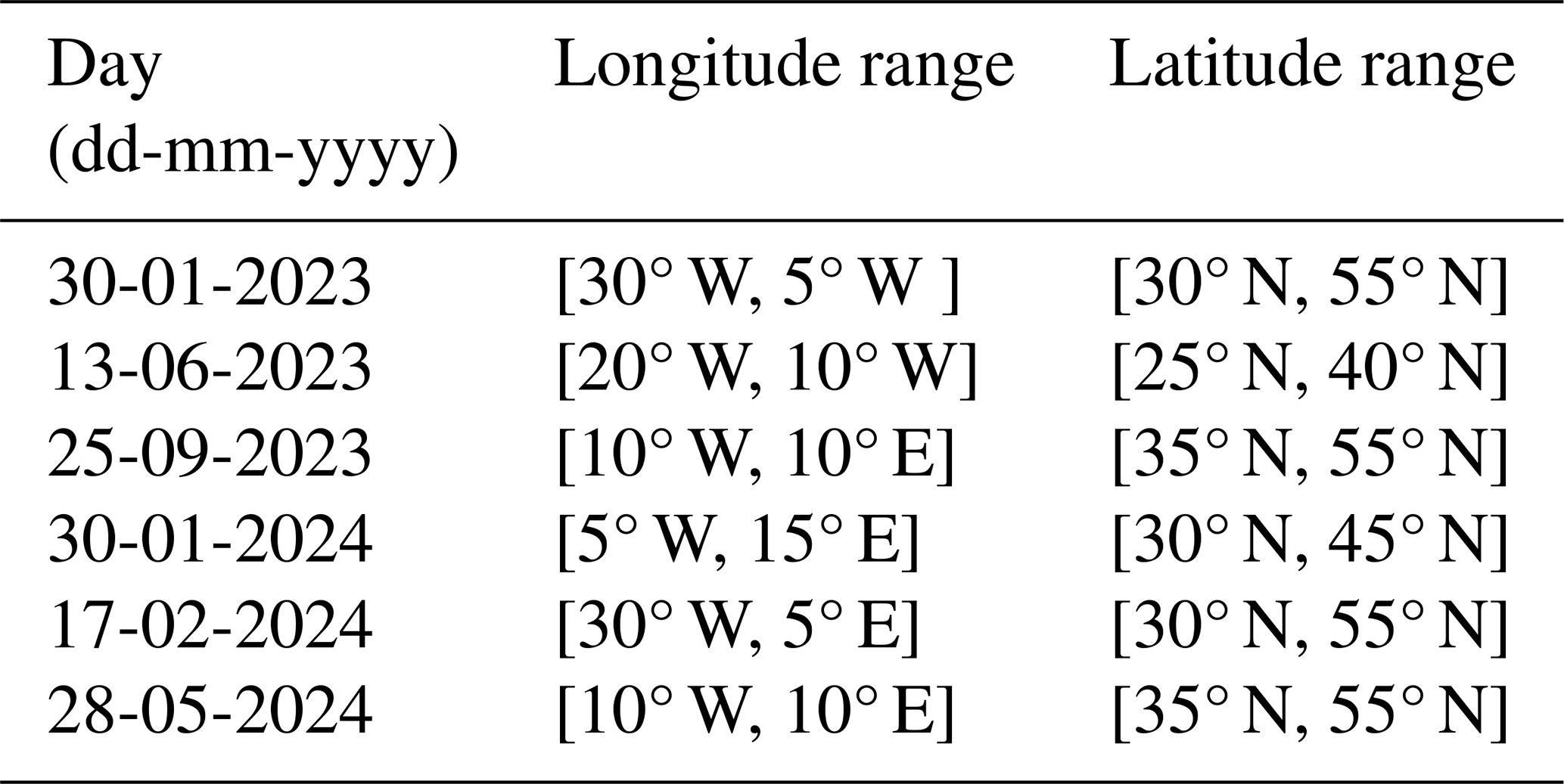
Figure 7 presents an example of the DUST/RGB composite from SEVIRI/MSG, focusing on the geographic region over France and the Bay of Biscay for 25 September 2023, from 06:00:00 to 07:15:00 UTC. It should be noted that, for the sake of visual clarity, Figs. 7, 8, and 9 demonstrate only a part of the zoomed geographic region where potential contrails are observed. At 06:00:00 UTC, a dense ice cloud is observed, surrounded by line-shaped ice clouds over the northern Bay of Biscay and France. As time progresses, the dense ice cloud mass disperses, while at the same time, we observe the formation of several line-shaped ice clouds around it.

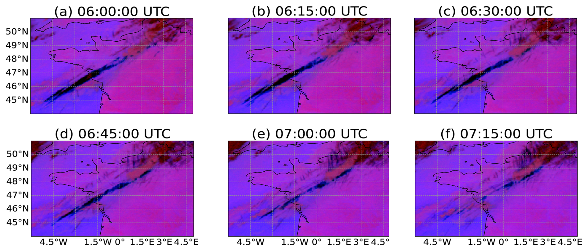
Figure 7 MSG/SEVIRI Dust/RGB images for an example date and sequence of observation times (25 September 2023) in a zoomed geographic area, where potential contrails are detected.

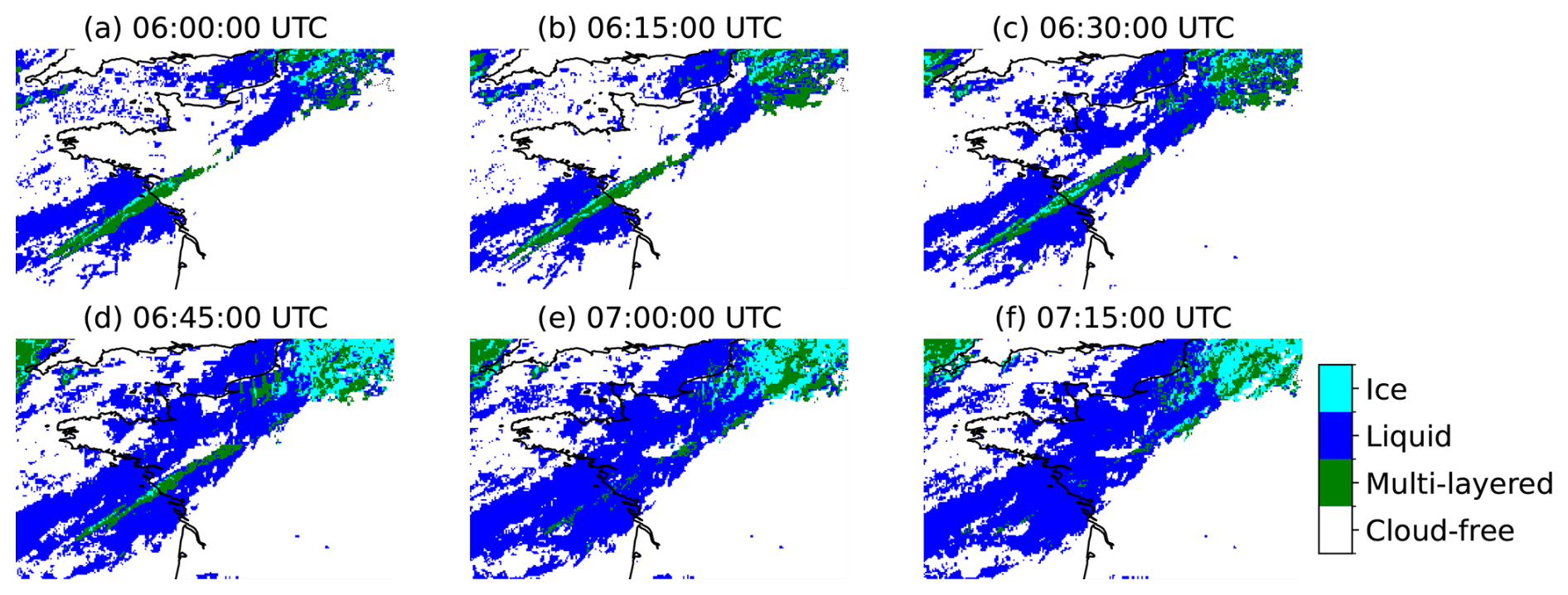
Figure 8 Cloud phase (cloud-free or multi-layered, liquid or ice cloud) as retrieved by the Optimal Cloud Analysis (OCA) algorithm for an example date and sequence of observation times (25 September 2023) in a zoomed geographic area where potential contrails are detected.

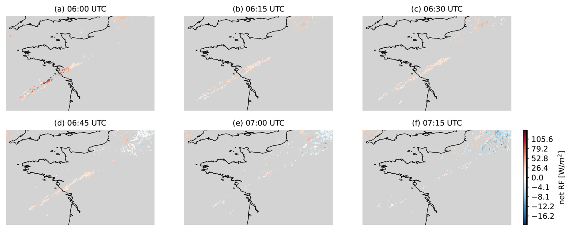
Figure 9 Net radiative forcing (RF) (sum of SW and LW RF) of potential contrails for an example date and sequence of observation times (25 September 2023) in a zoomed geographic area.

As it is demonstrated in Fig. 8, the OCA algorithm successfully detects the dense ice cloud at 06:00:00 UTC as a mixture of ice and multi-layered clouds. Interestingly, as time progresses, most of the formed line-shaped potential contrails are characterized as clouds by the OCA algorithm. We observe that many ice clouds are identified as clouds only in their central parts, while their thinner edges often remain undetected. We speculate that this is due to the spatial resolution of SEVIRI/MSG observations, which is 3 × 3 km² at the SSP.

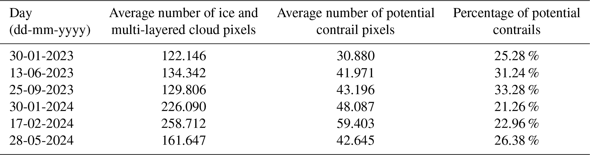
As presented in Sect. 3.2, the application of a CTP filter distinguishes natural cirrus clouds from potential contrails. In the following section, we proceed with the generation of RF maps based on this distinction. Table 3 summarizes the average number of pixels characterized as ice and multi-layered clouds for each selected day per observation, as well as the percentage of these pixels having potential contrails. The day with the largest number of potential contrail pixels is 17 February 2024, followed by 30 January 2024.

Table 3 Selected days, average number of ice and multi-layered cloud pixels, and average number of potential contrail pixels per observation, and percentage of cirrus over the overall geographic region.

4.2 Radiative forcing of potential contrails

From this section onward, the focus is exclusively on potential contrail clouds: a net RF value was assigned to the pixels characterized as ice or multi-layered clouds that passed the distinguishing filter between low- and high-altitude ice clouds, the latter representing potential contrails in this work.

The net RF is calculated as the sum of RF_sol + RF_tir. As discussed in Sect. 2.3, the presence of an ice cloud is most commonly expected to result in cooling in the SW wavelength region (negative RF values) and warming in the LW wavelength region (positive RF values).

Figure 9 presents maps of potential contrails net RF for the same geographic region as in Figs. 7 and 8 on 25 September 2023, from 06:00:00 to 07:15:00 UTC. For this sequence of observation times, the detected potential contrails exhibit a positive radiative effect, indicating that the overall effect was warming during these early morning hours. At 06:00 UTC, the long, thin ice cloud mostly located above the Atlantic exhibits the strongest warming effect compared to other ice clouds during the rest of the time period, likely due to the still nighttime conditions in this region. As daytime progresses and the sun rises, the warming effect of the potential contrails diminishes, indicating that the shortwave cooling effect becomes more pronounced.

An overall daily view of the RF effect of potential contrails is provided in Fig. 10. Over the geographic region of interest and for the 6 selected days, the net RF values of the detected ice or multi-layered cloud pixels have been multiplied by the coverage area per pixel, summed and then divided by the total coverage area for all the pixels. We refer to this summation as the total RF_ice. Additionally, summing up only the potential contrail pixels will provide us the total RF_contrail. For the example day of 25 September 2023 (Fig. 10c), the total net RF values of the potential contrails range from −3.71 W m⁻² (12:00 UTC) to 3.90 W m⁻² (23:30 UTC). As it is expected, for all the selected days, the maximum total net RF_contrail appears during nighttime due to the absence of SW cooling, while the minimum RF_contrail value occurs during daytime and close to each midday. Even though the largest number of potential contrail pixels is found during 17 February 2024, we observe that the absolute maximum RF_contrail values are observed during 13 June 2023 (see Table 3). This is due to the increased incoming solar radiation during the warmer months in the Northern Hemisphere compared to the colder months. Additionally, the contribution of the LW RF to the total RF for the detected ice and multi-layered clouds, and potential contrail pixels is presented in each subplot in Fig. 10. It is observed that, for each case, the LW consistently contributes positively to the total RF throughout the day, with small fluctuations observed across different cases.

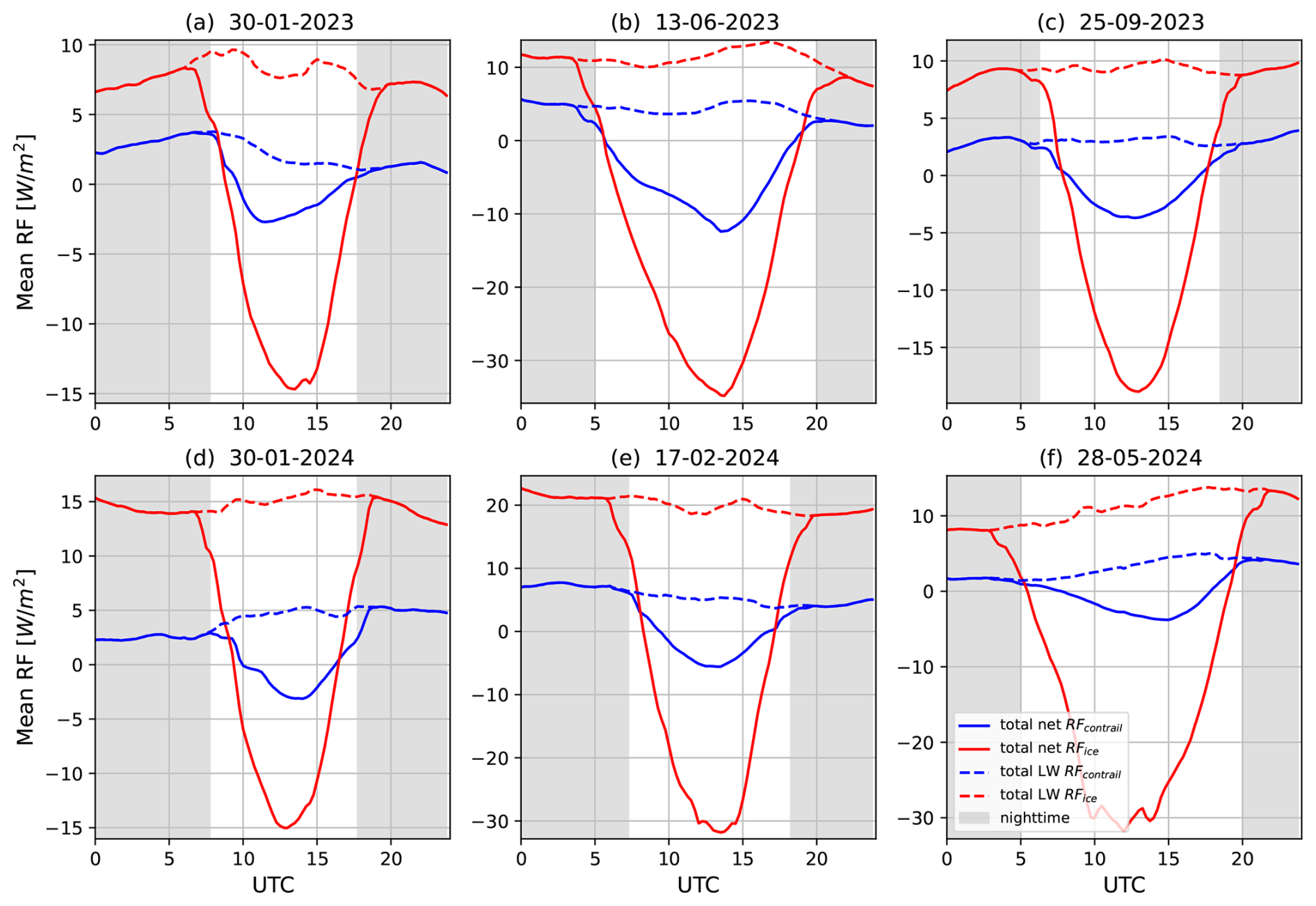
Figure 10 Time series of total net and longwave (LW) radiative forcing (RF) in W m⁻² for all the detected ice and multi-layered clouds (represented by solid and dashed red lines) and for only the potential contrails (represented by solid and dashed blue line) above the overall geographic area for the 6 selected days. The shaded grey background indicates nighttime.

5 Validation of the Rapid Contrail-RF Estimation Approach

The accuracy and reliability of the Rapid Contrail-RF Estimation Approach in constructing RF maps for high-altitude ice clouds, including potential contrails, have been investigated through five different validation exercises, presented in the following subsections. These exercises focus on different aspects of the methodology. First, we evaluate the choice of using a single atmospheric vertical profile in the RT simulations (Sect. 5.1). Next, by performing a small subset of RT simulations, we investigate the impact of selecting a certain ice cloud parameterization scheme (Sect. 5.2). Additionally, we evaluate the impact of using CTH values estimated by a single atmospheric vertical profile on the RF estimations (Sect. 5.3). Then, we perform a comparison between the flux maps for potential contrails and polar-orbiting satellite observations (Sect. 5.4). Finally, a comparison between our results and those reported in Wang et al. (2024) for two contrail cirrus outbreaks is also presented.

5.1 Impact of vertical temperature profile on radiative transfer calculations

The core component of the Rapid Contrail-RF Estimation Approach is the construction of the ice cloud RF LUTs and their merging with the re-gridded geostationary maps (see Sect. 3.1). As presented in Sect. 2.3, the atmospheric temperature vertical profile used in the RT simulations remains constant and corresponds to the U.S. Standard Atmosphere.

To assess the validity of this choice and estimate the uncertainty associated with using a single constant temperature vertical profile, randomly selected pixels from the zoomed geographic regions of each day-containing potential contrails above land, ocean, and liquid water clouds (i.e., multi-layered)-covering day- and night-time conditions were chosen as the sample of this investigation.

For these selected pixels, RT simulations were performed using the ERA5 vertical temperature profile from ECMWF (see Sect. 2.4) as the input atmospheric profile. These profiles were also used to estimate CTH and wCTH (only in the presence of a liquid water cloud). Additionally, for each pixel, the actual CER and COT values from the OCA product were used, along with the real SZA. In the presence of a liquid water cloud, we use the wCOT value from the OCA product.

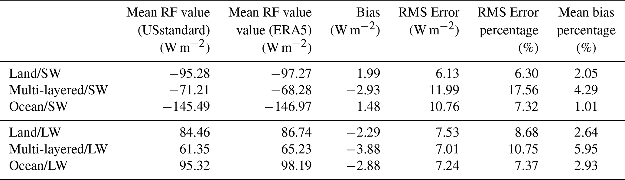
In Fig. 11, for each scene scenario, we present the comparison results between the RF values coming from the LUTs (RF_USstandard) and the RF values calculated by using the actual atmospheric and cloud conditions (RF_ERA5) per selected pixel in the SW and LW wavelength ranges, separately. As it can be seen, for all the scene scenarios in the SW wavelength range, overall good agreement is found with the correlation coefficient (R) ranging from 0.97 to 1.00 and slope (s) from 0.93 to 0.97, with the exception of a few comparison points. Table 4 provides some statistics for the two different methodologies followed in this Section per wavelength and scene scenario. In the SW wavelength range, the use of LUTs instead of real-time RT simulations per pixel can lead to RMS error percentage equal to 6.30 %, 7.32 %, and 17.56 % above land, ocean, and liquid water cloud, respectively. The comparisons in the LW wavelength range (see Fig. 11) reveal an overall good agreement with correlation coefficient values being around 1.00 and slope values in the range of 0.95–0.97. In contrast to the comparison in the SW, in the LW, we observe that a larger number of points appears to be scattered around the 1:1 line. This finding means that the RT simulations in the LW wavelength range are more sensitive in the choice of the atmospheric temperature vertical profile. The use of LUTs in the LW wavelength range leads to RMS error values of the same order of magnitude for the three scene scenarios. When focusing on the SW and LW RMS error percentage, we find that the largest values for both wavelength ranges are observed for the scene scenario of an ice cloud above a liquid water cloud (multi-layered).

Figure 11 Scatter plot between radiative forcing (RF) values estimated by using the Look-Up Tables (LUTs) (RF_LUTs) and radiative transfer calculations using the actual atmospheric temperature vertical profiles (RF_actual) for randomly selected pixels containing potential contrails above land surfaces in the (a) SW, and (b) LW, underlying liquid water clouds (i.e., multi-layered) in the (c) SW and (d) LW, and ocean surfaces in the (e) SW and (f) LW.

Table 4 Mean radiative forcing (RF) values over all the randomly selected pixels for the 6 selected days, bias, RMS error, RMS error percentage, and mean percent errors between RF values estimated by using the Look-Up Tables (LUTs) and by using the ERA5 atmospheric profile and the OCA cloud conditions for the SW, and LW estimated RFs.

To explain the scattered points around the 1:1 line in the subplots of Fig. 11, we focus on the points with an RMS error value larger than the mean RMS error value plus two times the standard deviation of the RMS error. For these points, we first investigated whether there is a correlation between the large discrepancies in the two RF datasets and the differences between the values of each actual cloud parameter and the closest values used during the multi-dimensional interpolations in the LUTs. The comparison results depicted no correlation.

Additionally, for these points, we examine the corresponding ECMWF vertical profiles used in the RTM simulations. Figure 12 illustrates the temperature and humidity of the US Standard profile, along with the median profile of the ECMWF vertical profiles, as well as the coverage of these profiles. We observe that the coverage of the ECMWF vertical profiles demonstrates different values for surface temperatures but their median profile agrees very well with the US Standard atmospheric profile. In contrast, the humidity ECMWF vertical profiles depict a large difference at the surface compared to the US Standard profile.

Figure 12 Vertical (a) temperature and (b) humidity profiles of US Standard atmosphere, median profiles of the ECMWF vertical profiles corresponding to the largest discrepancies (i.e., large RMS error percentage between radiative forcing (RF) values estimated by using the Look-Up Tables (LUTs) (RF_LUTs) and radiative transfer calculations using the actual atmospheric temperature vertical profiles) for the 6 selected days.

Overall, in the SW wavelength range, the use of a standard profile in the construction of the LUTs lead to mean bias percentage of about 2.05 %, 1.01 %, and 4.29 % for a contrail above land, ocean, and liquid water cloud, respectively. In the LW wavelength range, the mean percent errors equal to 2.64 %, 2.93 %, and 5.95 % for a contrail above land, ocean, and liquid water cloud, respectively.

5.2 Impact of ice cloud parameterization on radiative transfer calculations

The micro-physical properties of the ice crystals, which are part of the ice clouds, play a crucial role in their single scattering properties and, consequently, the RF of these clouds (Stephens et al., 1990; Sanz-Morère et al., 2020). Here, we assess the impact related to the choice of ice cloud parameterization in the RT simulations. The parameterization determines how the ice water content and CER are translated into optical properties. Since the ice crystal shape is an unknown parameter, we have selected the parameterization by Yang et al. (2013), assuming the ice crystal habit to be a column composed of 8 elements with a moderate degree of roughness, as this is the habit most frequently observed for thin ice clouds (Forster and Mayer, 2022) and contrails (Järvinen et al., 2018). According to the same study, 60 % of cirrus clouds are a mixture of ice crystals with severe roughness, while 40 % a mixture of smoothed ones. Similarly to Wolf et al. (2023), we have chosen a moderate degree of roughness for the simulations included in the LUTs.

For this sensitivity study, we performed a small subset of RT simulations in the SW and LW wavelength ranges, varying the choice of ice cloud parameterization. We selected all the available ice crystal shapes from the parameterization by Yang et al. (2013). In addition, we included the parameterization by Fu (1996), and by Fu et al. (1998), which is operationally applied in the ECMWF Integrated Forecasting System (IFS) and assumes ice crystals as pristine hexagonal columns. The simulations are always performed for an ice cloud with a COT equal to 0.5 to maximize its semi-transparency and, subsequently, the effect of cloud microphysics. We have chosen three different SZA values (10, 40, and 70°), a CER of 20 µm, and a CTH of 10 km. For these simulations, the ice cloud is located above an ocean surface characterized by three different SST values (273, 293, and 303 K).

Figure 13 presents RF_sol as a function of various ice crystal habits based on the parameterization of Yang et al. (2013) (i.e., column with 8 elements, droxtal, hollow bullet rosette, hollow column, plate, plate with 10 elements, plate with 5 elements, solid bullet rosette, and solid column) and their degrees of roughness (smooth, moderate, and severe) for three different SZAs. The ice crystal habit of an hexagonal column by Fu (1996) is included as well. Additionally, the figure presents the relative differences in RF_sol compared to the selected ice crystal shape and degree of roughness for the construction of the LUTs. As observed, the choice of ice crystal habit and roughness degree can result in large differences, which can be up to 60 % (e.g., the case for SZA = 10° for smooth plates of 10 elements) in the SW wavelength range. In addition, the parameterization of Fu (1996), which assumes a pristine hexagonal column results in differences up to approximately 20 % for the case of a small SZA. For the three SZA scenarios, RF_sol of the selected ice crystal shape and roughness appears to have the lowest values compared to other ice crystal shapes and degrees of roughness.

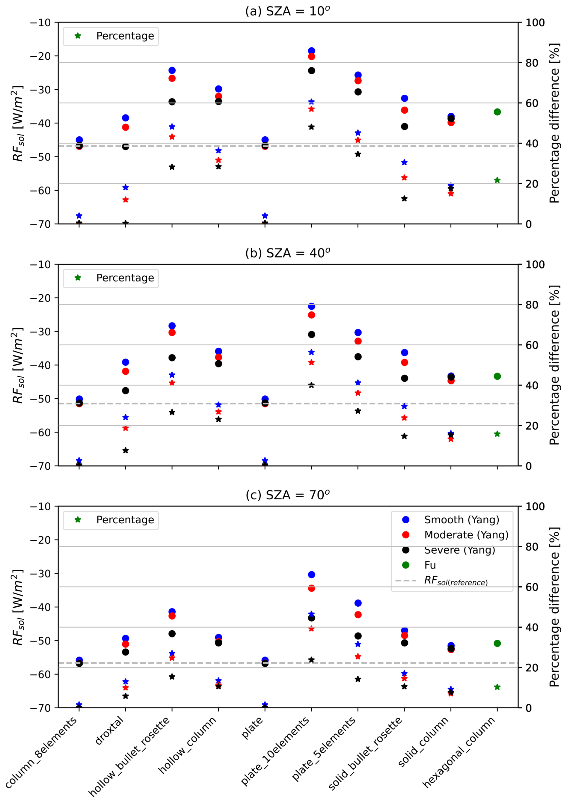
Figure 13 Simulated radiative forcing values in the shortwave (i.e., solar) wavelength range (RF_sol) are presented as a function of various ice crystal habits and their degrees of roughness (shown with circles) based on the parameterization of Yang et al. (2013) and Fu et al. (1998) for three different solar zenith angle (SZA) scenarios. The horizontal line (i.e., grey dashed line) represents the RF_{sol(reference)} value for the selected ice crystal shape and roughness used in this study. The percentage difference between each ice crystal habit and the one used in the LUTs is denoted by star symbols.

Figure 14 presents RF_tir as a function of the same ice crystal habits and roughness degrees for three different SST scenarios, along with their relative differences. In contrast to the shortwave range, the differences in the LW (RF_tir) are much smaller, not exceeding 12 %.

Figure 14 Similar as Fig. 13 but for the longwave (i.e., thermal infrared) wavelength range, where RF_tir values are presented for three different sea surface temperature (SST) scenarios.

From the sensitivity tests, we conclude that ice crystal habit and roughness can lead to significant differences in RT simulations in the SW wavelength region, while these factors play a less significant role in the LW wavelength region. When investigating the simulated upward and downward irradiance at TOA in the SW wavelength region, we find that the largest differences between the selected ice crystal shape and roughness (i.e., column of 8 elements with moderate roughness) and a plate of 10 elements with a smooth degree of roughness (i.e., largest differences in RF_sol) occur in the following wavelength ranges: 1122–1135, 1346–1471, 1800–1954, and 2486–2752 nm. Similarly, in the LW wavelength, the simulated spectrum is affected the most by the choice of the ice crystal shape and roughness in the following wavelength ranges: 3487–4171, 4645–5502, and 8113–9153 nm.

To estimate the uncertainty associated with the selection of a specific ice cloud parameterization in the RF_sol and RF_tir maps, we have re-performed the RT simulations for the randomly selected pixels (see Sect. 5.1 for only a single day; 25 September 2023). Consequently, the comparison is made between RF_sol and RF_tir obtained in Sect. 5.1, where the default ice cloud parameterization was applied, and those generated by employing the same input values for the RT simulations, but differing the choice of ice cloud parameterization. For the comparison, we have used the ice crystal habit and roughness, which exhibits the largest difference with our default settings: plate of 10 elements with a smooth degree of roughness (Yang et al., 2013).

Table 5 summarizes the findings of the above-mentioned comparison. As expected by the sensitivity study, the use of another ice crystal habit and roughness can lead to large differences in the SW and slightly affects the LW wavelength range. For the SW wavelength range and for all the scene scenarios, the mean RF values for columnar and plate ice crystals differ by a negative bias, with the largest bias found for contrails above ocean surfaces (−49.33 W m⁻²).

Table 5 Mean radiative forcing (RF) values over all the randomly selected pixels for 25 September 2023, bias, RMS error between RF values when using an ice crystal habit of column with 8 elements and a plate with 10 elements for the SW, LW, and net estimated RFs.

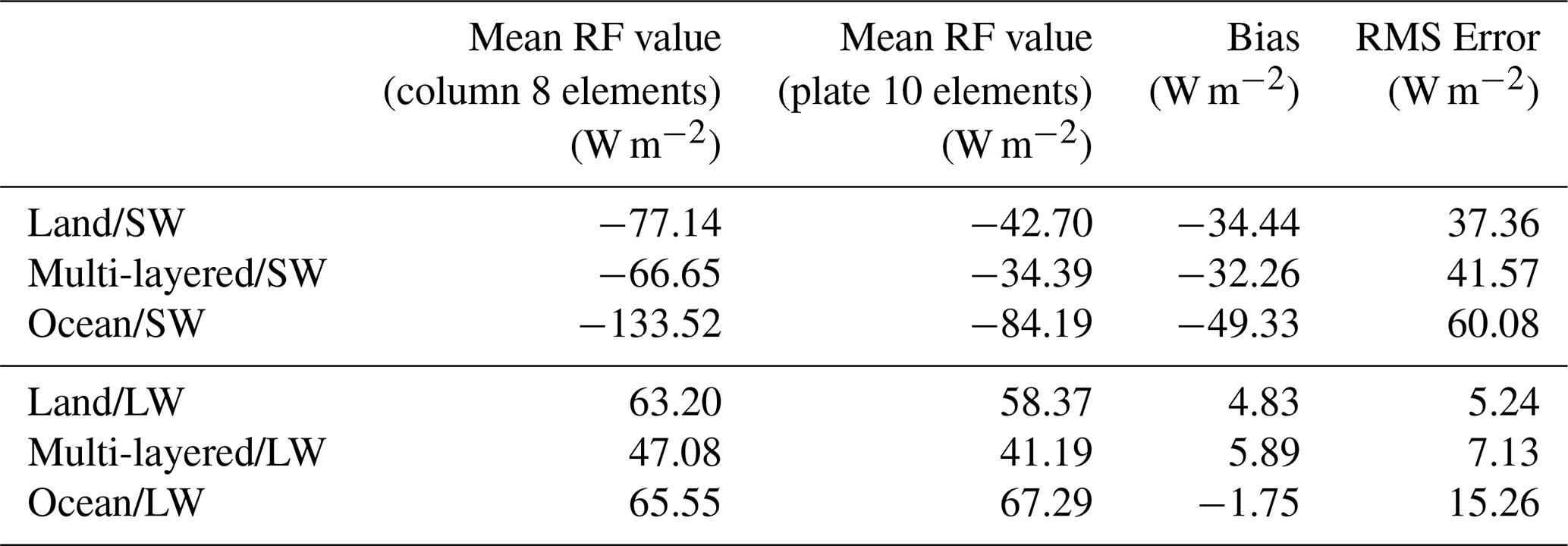
For the LW wavelength range, the bias values are smaller, with the largest bias being equal to 5.89 W m⁻² for ice clouds above liquid water clouds (i.e., multi-layered).

We should keep in mind that actual measurements of the micro-physical properties of ice crystals in contrail clouds are rare and difficult to obtain. There have been in situ measurements, such as those in Järvinen et al. (2018), which found that the primary ice crystal habit is aggregates (i.e., the one used in this study), though the presence of other crystal shapes has been reported. Consequently, we used the most common one to optimize the representation of ice crystals. However, applying a single ice crystal shape and roughness for the overall number of potential contrails during different seasons, and above various scenes may not be fully representative.

5.3 Impact of Cloud Top Height (CTH) on radiative forcing interpolation

As mentioned in Sect. 2.2, the OCA product provides the CTP. To have the information about CTH, which is used as a parameter in the RT calculations in the LW wavelength range, the US Standard profile is used. More precisely, we linearly interpolate the CTP in the pressure vertical grid, and consequently, the altitude vertical grid, of the US Standard atmospheric profile.

CTH plays an important role in the LW wavelength range, where it is utilized to perform the multi-dimensional interpolation of the simulated RF_tir values from the LUT at the actual values of the cloud and environmental parameters for each pixel. To evaluate the accuracy of using a constant atmospheric profile to estimate the CTH, we have selected the same pixels as in Sect. 5.1. For these pixels, ECMWF pressure vertical profiles were used to interpolate linearly the potential contrail CTP in the altitude vertical grid of those profiles. Consequently, this CTH value, named “CTH − ECMWF”, in every selected pixel can be used to re-perform the multi-dimensional interpolation in the parameters and estimate a new RF value in the LW wavelength range.

Figure 15 presents the comparisons between this new RF value by using the actual CTH and a CTH estimated by the US Standard profile. As we can see, the correlation between them is excellent for the three different scene scenarios, indicating that using a different CTH value does not affect the multi-dimensional interpolation performed in the LUTs to extract the RF_tir. As it is demonstrated in Fig. 16, for the three different scene scenarios, the CTH values estimated by using a real atmospheric and the US Standard profile depict small differences with a mean bias equal to 0.85 %, −0.60 %, and −1.70 % above land, ocean, and liquid water cloud, respectively. The scatter plots of Fig. 16 reveal that for the three scene scenarios, CTH estimated by the US Standard profile is systematically lower by 22 %–26 % compared to the CTH estimated by the ECMWF vertical profiles.

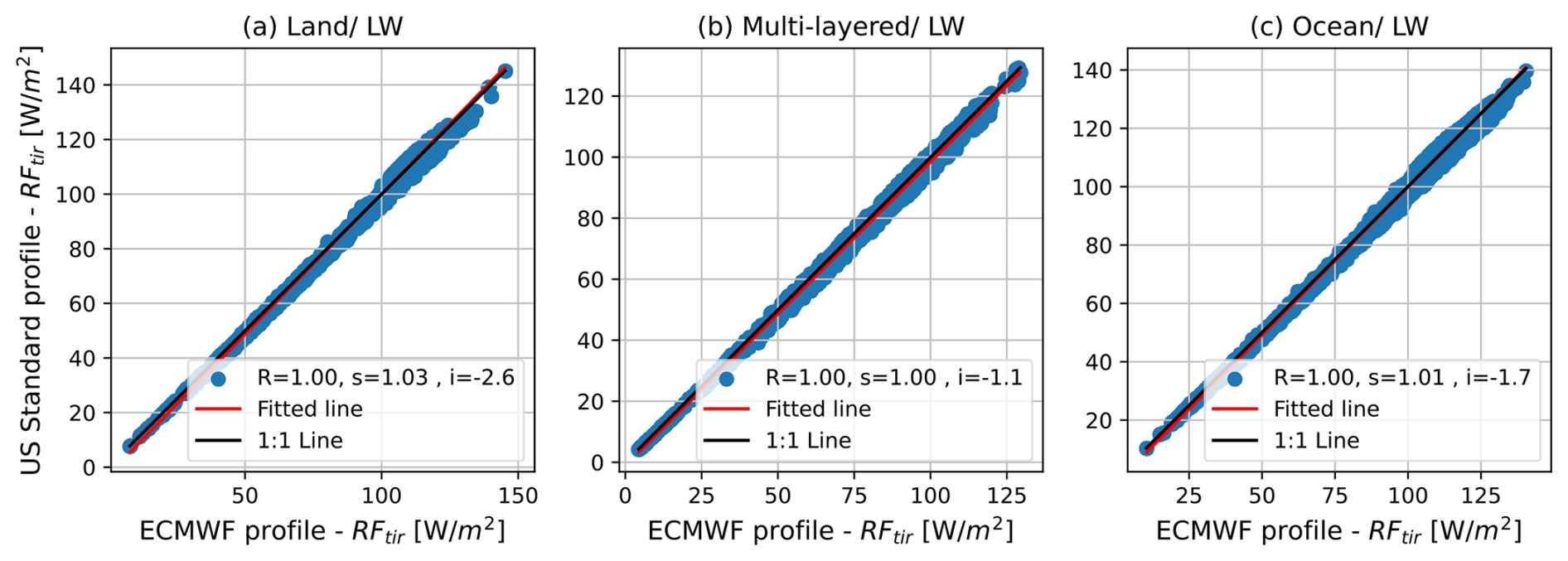
Figure 15 Scatter plots between radiative forcing (RF) values estimated by using the cloud top height (CTH) as estimated by the US Standard profile and by the ECMWF temperature profiles for randomly selected pixels containing potential contrails above (a) land surfaces, (b) underlying liquid water clouds and (c) ocean surfaces in the LW wavelength range.

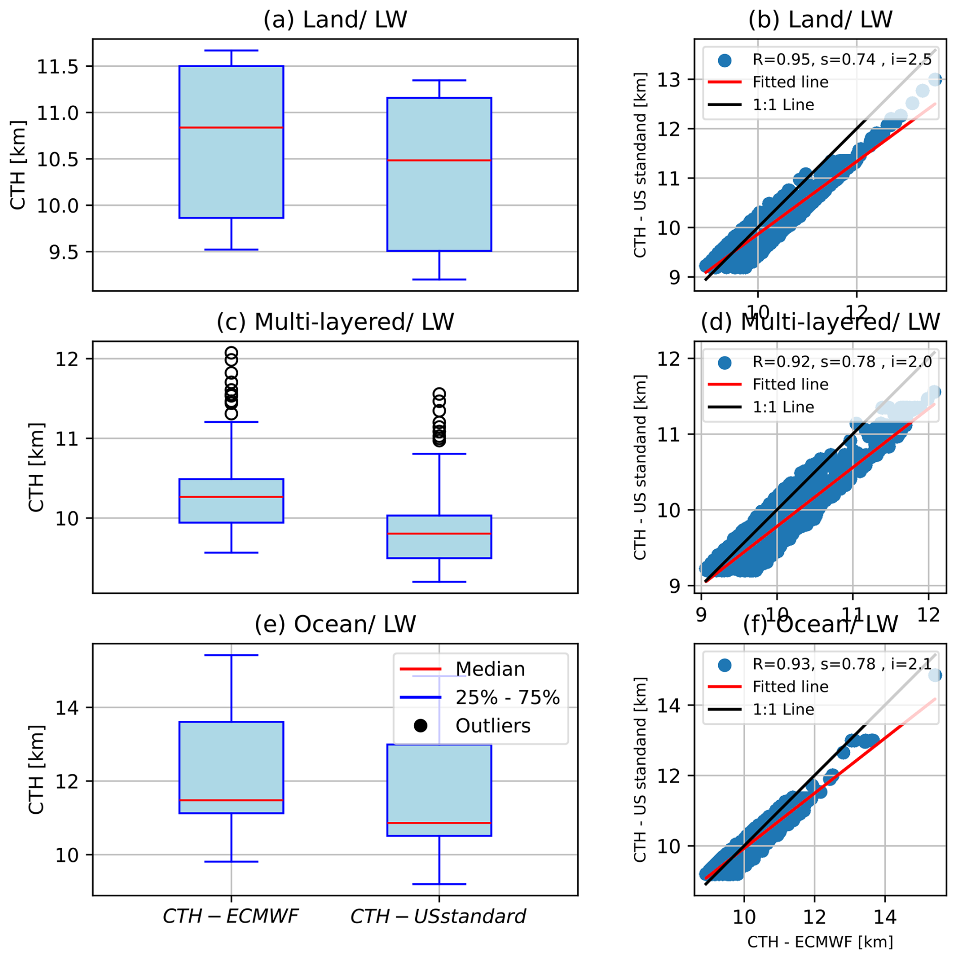
Figure 16 Box-Whisker plots of cloud top height (CTH) values as estimated by the US Standard profile and by actual temperature profiles from ECMWF for randomly selected pixels containing potential contrails above (a) land surfaces, (b) underlying liquid water clouds and (c) ocean surfaces in the LW wavelength range.

5.4 Comparison of estimated flux maps and CERES observations

TOA upward solar (i.e., SW) and thermal infrared (i.e., LW) fluxes, as observed by the CERES FM1 and FM3 instruments, have been used to validate the first output after merging the datasets in the Rapid Contrail-RF Estimation Approach: the TOA upward SW and LW fluxes referred to as F_up (see Eq. 1). This comparison focuses exclusively on pixels identified as potential contrail pixels.

The comparison was conducted using data from the 6 selected days. For each of these days, the closest-in-time MSG/SEVIRI observation was matched with the CERES observations (approximately four per day above the zoomed geographic region of interest) by taking into account the exact acquisition time of the selected MSG/SEVIRI pixels. Since CERES has a larger footprint (approximately 25 km in diameter near nadir) compared to the spatial resolution of the flux maps generated by the Rapid Contrail-RF Estimation Approach, we averaged the potential contrail pixels, which are located inside the CERES footprint. To perform this averaging, we defined an ellipsoid area around the latitude and longitude of CERES field-of-view (FOV) at surface, based on the satellite's height, viewing zenith angle, and the clock angle of CERES FOV at satellite. If this area was covered of potential contrail pixels more than 75 %, we averaged these pixels and compared them with the CERES fluxes in the SW and LW wavelength ranges, separately.

Figure 17 presents the outcome of the comparison described above. As seen, there is generally good agreement in the SW and LW wavelength range, with a correlation coefficient (R) of 0.99 and 0.86, respectively.

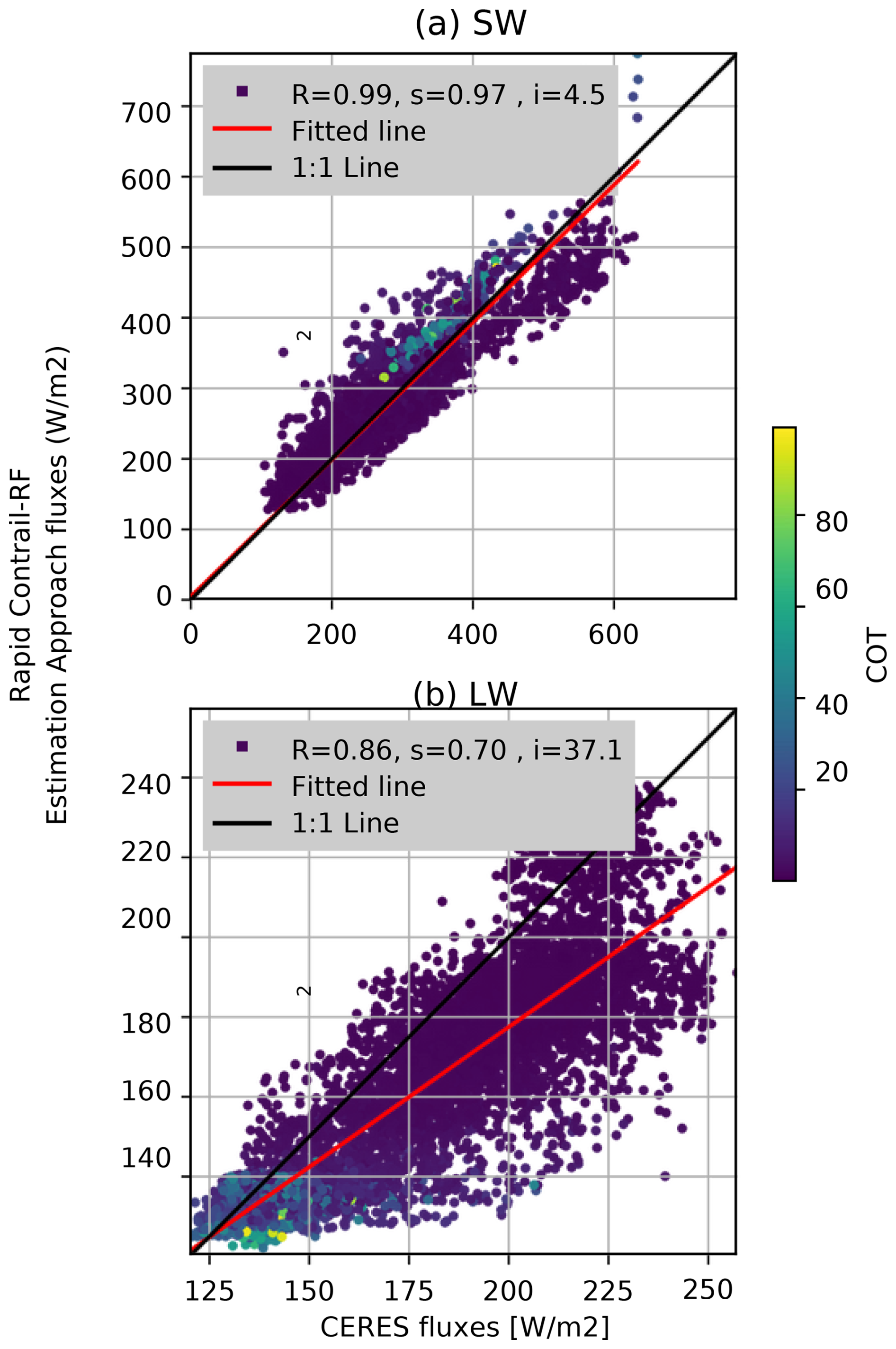
Figure 17 Scatter plots of TOA fluxes observed by CERES and estimated by using the LUTs in the shortwave (SW, upper plot) and longwave (LW, lower plot) wavelength ranges. The points of each plot are color-coded based on the mean potential contrails optical thickness (COT for cloud optical thickness), averaged within the respective CERES footprints.

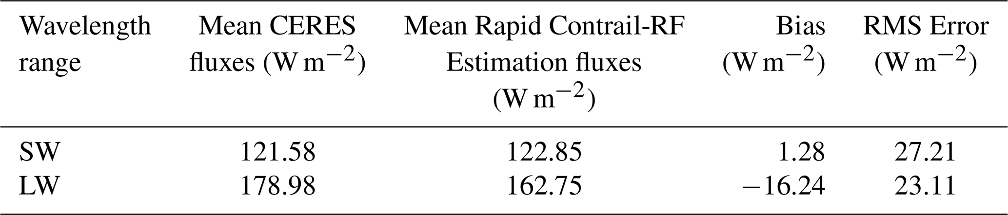
Table 6 provides overall statistics for the mean CERES and Rapid Contrail-RF Estimation-estimated upwards TOA fluxes. The bias in the SW wavelength range (1.28 W m⁻²) indicates that the Rapid Contrail-RF Estimation Approach, in general, slightly overestimates the SW fluxes by 1.05 % compared to CERES, while in the LW wavelength range the bias is negative (−16.24 W m⁻²) indicating that our approach underestimates in general the LW fluxes by 9.07 % compared to CERES. Additionally, the higher Rapid Contrail-RF Estimation Approach SW fluxes compared to CERES align with the RF_sol values for the ice cloud microphysics in Sect. 5.2. There, it was demonstrated that using column of 8 elements as the ice crystal shape results in the lowest radiative forcing values compared to other ice crystal shapes. Concerning the RMS error, the Rapid Contrail-RF Estimation Approach seems to perform better in estimating LW fluxes than SW ones. However, we observe that in LW wavelength range, the two compared fluxes exhibit the largest scattering, resulting in many points having considerably lower fluxes compared to CERES ones.

Table 6 Mean CERES and Rapid Contrail-RF Estimation Approach-estimated upwards TOA fluxes, bias and RMS error for the SW and LW wavelength range.

Focusing on the mean cirrus optical thickness (COT) values, averaged within the respective CERES footprints and color-coded in Fig. 17, we observe that in the LW wavelength region, the largest COT values correspond to cases in which the Rapid Contrail-RF Estimation Approach retrieves low fluxes (smaller than 140 W m⁻²), while the CERES fluxes demonstrate larger variability. In the SW wavelength, there is no direct correlation between mean potential contrail optical thickness values and discrepancies between the two datasets.

5.5 Comparison with an existing study

A direct comparison has been conducted between the outputs of the Rapid Contrail-RF Estimation Approach and the results reported in Wang et al. (2024). In that study, the authors investigated the radiative effects of two contrail cirrus outbreaks over Western Europe using geostationary satellite observations and radiative transfer calculations. Our primary motivation for this specific comparison is the use of a common geostationary satellite and cloud product (a modified OCA product; see below).

The two outbreaks extended over Western Europe on 2 consecutive days, 22 and 23 June 2020. For these days, Dust/RGB images from the MSG/SEVIRI satellite were used to visually demonstrate the two outbreaks. We now describe the methods used by the authors of Wang et al. (2024): radiative transfer simulations were then conducted using ecRad as the radiative transfer code. The required input for ice cloud properties was derived from the OCA product, modified by increasing the COT values by a multiplicative factor of 1.3. The ice crystals were assumed to be pristine hexagonal columns. Atmospheric vertical profiles were obtained from the ECMWF Reanalysis version 5 (ERA5). Consequently, both studies share common components in their methodology but also exhibit important differences.

Figure 18 shows the net RF values of the contrails during the first outbreak from 09:00 to 22:00 UTC on 22 June 2020, focusing on the same geographic region as in Wang et al. (2024). This figure corresponds to Fig. 2 in Wang et al. (2024). A first qualitative comparison between the two figures clearly reveals the warming effect of contrails over land. However, in our case, at 12:00 UTC, we observe mainly cooling over ocean, whereas in Wang et al. (2024), the ice clouds exhibit both cooling and warming effects. At 18:00 UTC, the pattern is reversed.

Figure 18 Maps of the net radiative forcing (RF) of ice clouds over the study region presented in (Wang et al., 2024), shown at six different times on 22 June 2020.

We conducted a quantitative comparison to assess the net total power of the SW, LW, and net RF of ice clouds and clouds with CTP above 300 hPa, expressed in terrawatt (TW), over the region of interest from 07:00 UTC on 22 June 2020 to 12:00 UTC on 23 June 2020. We used the online tool WebPlotDigitizer (https://automeris.io/, last access: 28 October 2025) to extract the SW, LW, and net total radiative effect of the both the ice clouds and those located above 300 hPa from Figs. 3b, S6a, and S6b in Wang et al. (2024), which we could then compare directly to our own values. As shown in the comparisons in Fig. 19, both datasets,total ice clouds and above 300 hPa, exhibit excellent agreement in terms of correlation coefficient values for SW, LW and net total power over the geographic area of interest. However, the Rapid-Contrail Estimation Approach systematically yields smaller values compared to the results of Wang et al. (2024) as reflected in the slope values in Fig. 19.

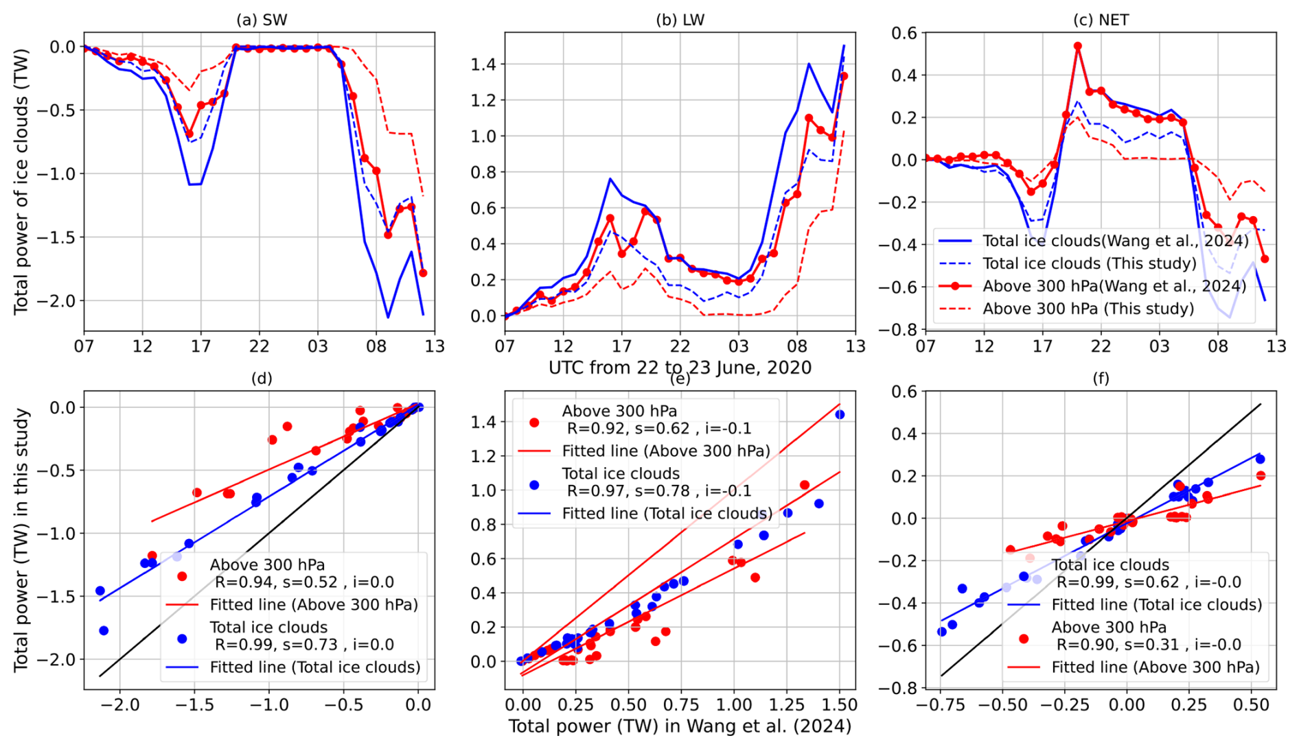
Figure 19 Time series of SW (a), LW (b), and net (c) total power of the ice cloud radiative effect over the study region from 07:00 UTC on 22 June 2020 to 12:00 UTC on 23 June 2020, for both the total ice cloud amount (blue lines) and ice clouds located above 300 hPa (red lines) in the two studies. Panels (d)–(f) show scatter plots comparing the total power values reported in Wang et al. (2024) and those obtained in this study for the SW (d), LW (e), and net (f) wavelength ranges.

6 Conclusions

Quantifying the radiative forcing of contrails remains an active area of research, primarily due to significant uncertainties surrounding their overall contribution to climate change. In this study, we present and evaluate a new satellite-based approach for mapping the radiative forcing of high-altitude ice clouds, including potential contrails. The so-called Rapid Contrail-RF Estimation Approach combines geostationary satellite observations, a cloud properties retrieval algorithm, radiative transfer modeling and a simple filtering scheme to distinguish high-altitude ice clouds.

For 6 selected days within the 2023–2024 period, during which potential contrails were visually identified, MSG/SEVIRI data in combination with the OCA product were used for the detection and characterization of potential contrail clouds and aviation-induced cloudiness. The central focus of this study is the application of pre-computed RF LUTs for thin to semi-transparent ice clouds in both SW and LW spectral regions. SW and LW RF values were assigned to pixels identified as ice clouds using a multi-dimensional interpolation scheme. This methodology is computationally fast, avoiding the need for real-time radiative transfer simulations, and enabling the processing of large datasets.

The primary aim of this study was to evaluate the validity and limitations of using RF LUTs in this context. This evaluation was conducted through five different validation exercises. The first three focused on (1) the choice of using a single atmospheric vertical profile for the LUTs construction, (2) the choice of using one single ice cloud parameterization scheme and finally, and (3) the impact of using CTH values estimated with a standard profile during the merging of the cloud product with the LUTs. The fourth validation exercise is an end-to-end validation, comparing potential contrail flux maps generated by the Rapid Contrail-RF Estimation Approach with those derived from CERES instruments. Finally, the fifth validation is a comparison between our results and those reported in Wang et al. (2024) for two contrail cirrus outbreaks is also presented.

The main findings of the first three validation exercises are as follows:

• 1.

  Using a single standard atmospheric profile – in this study, the US Standard atmospheric profile – for constructing RF LUTs generally provides promising results over the region of interest. Indeed, this assumption can introduce biases of up to −2.93 and −3.88 W m⁻² in the SW and LW wavelength range, respectively, which are considerably smaller compared to the respective fluxes.

• 2.

  Using a single ice crystal habit – in this study, a column composed of 8 elements with a moderate degree of roughness – for constructing the RF LUTs can lead to significant differences in the SW wavelength region. In the LW wavelength region, RF values are less sensitive to this selection. Using the most extreme difference scenario, which does not necessarily reflect reality, the choice of ice crystal habit can result to biases of up to −49.33 and 5.89 W m⁻² in the SW and LW wavelength range, respectively.

• 3.

  Using a CTH estimated from a single standard atmospheric profile during the merging of the cloud product with the RF LUTs leads to small differences in the LW wavelength range (i.e., biases of up to −1.70 W m⁻²).

The end-to-end validation, which compared potential contrail cirrus flux maps generated by the Rapid Contrail-RF Estimation Approach with those derived from CERES instruments, yielded encouraging results concerning the performance of the Rapid Contrail-RF Estimation Approach. The mean biases are found to be 1.28 and −16.24 W m⁻² for the SW and LW wavelength ranges, respectively. The observed biases can be partially attributed to the selected ice crystal habit, as the chosen habit tends to produce the lowest RF values compared to the other options.

Averaging all the mean biases percentage from the different correlative comparison in the LW and SW wavelength ranges, we find that our approach provides accurate data for estimating the radiative forcing of high-altitude ice clouds, including contrails, with an accuracy on the order of approximately 15 %.

The resulting potential contrail RF maps revealed that, for the 6 selected days in this study, the presence of these potential contrails causes warming during nighttime and cooling during daytime. The total daily mean net RF values caused by these potential contrails over the entire geographic area of this study were calculated as follows: 0.68 W m⁻² (25 September 2023), 0.25 W m⁻² (28 May 2024), 1.86 W m⁻² (30 January 2023), −2.31 W m⁻² (13 June 2023), 1.86 W m⁻² (30 January 2024), and 2.46 W m⁻² (17 February 2024). During the only summer month included in the analysis, the total daily mean net RF value is negative indicating that the SW contribution to the net RF in larger than the LW contribution. This is due to the increased incoming solar radiation during the warmer months in the Northern Hemisphere compared to the colder months. The total daily mean net RF values caused by these potential contrails over the entire geographic area of this study were calculated as follows: 0.68 W m⁻² (25 September-2023), 0.25 W m⁻² (28 May 2024), 1.86 W m⁻² (30 January 2023), -2.31 W m⁻² (13 June 2023), 1.86 W m⁻² (30 January 2024), and 2.46 W m⁻² (17 February 2024). During the only summer month included in the analysis, the total daily mean net RF value is negative indicating that the SW contribution to the net RF in larger than the LW contribution. This is due to the increased incoming solar radiation during the warmer months in the Northern Hemisphere compared to the colder months.

To conclude, our study presents a new satellite-based radiative forcing mapping of high-altitude ice clouds, including potential contrails. Performing various validation exercises, we demonstrate that this method provides reliable SW, LW and net RF maps for potential contrail clouds. Based on these findings, future steps could include extending this study to cover a full year, which we believe will offer valuable insights into the seasonal behavior of contrails. Furthermore, leveraging more advanced geostationary satellites with higher spatial and temporal resolution, such as Meteosat Third Generation/ Flexible Combined Instrument (MTG/FCI) would contribute in a better detection and monitoring of contrails. Finally, implementing an improved separation scheme between contrails and naturally occurring ice clouds – such as contrail detection algorithms based on neural networks (Ortiz et al., 2025) – is a necessary further step to perform radiation forcing studies for aviation-induced cloudiness.