Automatic methane plume masking based on wavelet transform image processing: application to MethaneAIR and MethaneSAT data

Efficient and accurate detection and masking of emission plumes are essential for localizing and quantifying point-source emissions via remote sensing. This study presents an automated plume-masking method based on a 2D discrete wavelet transform and advanced image conditioning processes, designed to replace workflows that rely on manual human identification. The method applies a 2D discrete wavelet transform to a methane concentration enhancement image, without assuming prior knowledge of source locations, enhancing plume features while suppressing background noise. The resulting binary plume masks are refined using information from distributions of concentration enhancements, plume morphology, and wind directions. Tunable parameters enable the algorithm to maintain high detection accuracy under varying background and meteorological conditions. The algorithm detected 75 % more plumes than previous methods when applied to MethaneAIR and MethaneSAT images while reducing false positives, primarily by improving sensitivity to low emission sources. Enhanced sensitivity provides more comprehensive emission rate distributions. The wavelet method is computationally efficient compared to machine learning models. It is designed to be readily adaptable to multiple aircraft and satellite platforms and to be applicable to other trace gases that exhibit plume-like structures associated with discrete sources.

1 Introduction

Detection of point sources of methane has progressed rapidly using remote sensing by airborne and spaceborne imaging spectroscopy in the shortwave infrared (SWIR). Previous studies have demonstrated the methane point source detection capabilities of satellites, including TROPOMI, Sentinel-2, Landsat-8/9, GHGSat, WorldView-3, PRISMA, EnMAP and EMIT (Cusworth et al., 2019; Ehret et al., 2022; Sánchez-García et al., 2022; Thorpe et al., 2023; Guanter et al., 2015). The launches of MethaneSAT and Carbon Mapper in 2024 further advanced methane monitoring efforts by contributing more point source data (Duren et al., 2025; Williams et al., 2026; Guanter et al., 2026, 2025). As more instruments and platforms become available, efforts are being directed toward creating open-source methane point source databases for stakeholders, policymakers, and the public. These efforts necessitate efficient and accurate methane plume detection and quantification methods with low computational cost and minimal human intervention.

A typical methane plume detection and quantification method generally involves two steps: (1) retrieving methane concentrations from radiance data, and (2) detecting point sources and inferring flux rates based on methane concentrations (Jacob et al., 2016, 2022). The second step often requires defining the plume boundary (mask), which is also a crucial input for visualizing plumes, and can also support localizing sources (origins). However, the retrieved plume concentrations are not always markedly higher than the background, due to either low plume concentration enhancements or background interference (such as upwind emissions and surface heterogeneity). Consequently, plume masking in practice still depends heavily on human inspection, making the process time- and labor-intensive (Thompson et al., 2015; Guanter et al., 2021). Reliance on manual input creates a bottleneck that increases the cost and time needed for plume detection. Furthermore, human inspection may introduce inconsistencies or subjectivity in plume boundaries, which increases the uncertainty and may lead to bias in quantification results.

The most common approach to plume masking involves simple thresholding, typically based on concentration values (Duren et al., 2019), percentiles (Sánchez-García et al., 2022), standard deviations (Chulakadabba et al., 2023), significance tests (Varon et al., 2018), or signal-to-noise ratio (Kuhlmann et al., 2024). The thresholding is often supplemented with pixel smoothing techniques, such as median filtering, Gaussian filtering, or mask dilation (Varon et al., 2018; Sánchez-García et al., 2022; Chulakadabba et al., 2023). Additional parameters, such as maximum plume length or minimum plume size, are sometimes applied to further reduce artifacts (Duren et al., 2019). The effectiveness of thresholding is often hindered by background interference and background noise, which is related to various factors such as upwind emissions, surface features, atmospheric conditions, and instrument sensitivities, creating a plume detection dilemma: if we report detections of plumes with relatively low enhancement (i.e., “weak” plumes), we engender a high rate of false detections.

Another type of plume masking approach involves computer vision machine learning (ML) models, which automatically generate plume masks by learning from labeled methane concentration maps (Jongaramrungruang et al., 2022; Radman et al., 2023; He et al., 2024; Rouet-Leduc and Hulbert, 2024; Růžička et al., 2023). However, these ML models still have several limitations. Firstly, their performance heavily depends on the size and quality of the training dataset, which may not always represent real-world conditions. Secondly, published results often report non-negligible rates of false positives (FPs) and false negatives (FNs). In addition, the demand for a large training dataset of ML models results in high computational costs. Furthermore, these models typically need retraining to adapt to different instruments or platforms, though some studies have reported consistent performance across different datasets without retraining (Růžička et al., 2023). Additional limitations include limited interpretability, uncertainty propagation, and biases toward the mean.

We present here an alternative method that is both computationally efficient and less dependent on training data, based on wavelet denoising. The 2D discrete wavelet transform is an image processing technique commonly used for image denoising and compression. It applies both high-pass and low-pass filters along the two spatial dimensions of an image, decomposing it into low- and high-frequency components. The low-frequency component retains the overall structure, while the high-frequency components capture finer details.

In atmospheric science, wavelet transform has been used mainly for decomposing time-series variations of gases and pollutants. In remote sensing applications, wavelet transform has been applied primarily for object detection and removal, such as identifying and eliminating haze and clouds from optical satellite imagery (Schneising et al., 2023). Wavelet-based methods have also been extended to hyperspectral data (Rasti et al., 2018), including full-spectra denoising approaches (e.g., 3D wavelets), which leverage spectral redundancy for noise reduction (Rasti et al., 2017). However, studies focusing on methane detection using wavelet transform remain limited. Among the few, Xiao et al. (2020) used wavelet transform to detect singularities in SWIR bands from the Shortwave Airborne Spectrographic Imager (SASI) and identify methane absorption features. Scafutto and De Souza Filho (2018) applied a Difference of Gaussians (DoG) wavelet to reduce noise in methane emissivity imagery derived from midwave infrared (MWIR) airborne hyperspectral data. Previous studies have not yet applied wavelet transform specifically for plume masking in SWIR-retrieved methane concentration maps.

In this study, we define a plume as a connected region of enhanced methane concentration that enables source localization and flux estimation from a discrete source. This definition includes plumes with a clearly identifiable hotspot or a physically consistent downwind shape that allows inference of the emission source location. We introduce an automated methane plume masking method based on wavelet transform. First, noise signals are extracted and subtracted from the input image to produce an enhanced image with enhanced plumes. Binary plume masks are then generated from this processed image using a combination of thresholding and a connected-component algorithm. Subsequently, a series of mask filtering techniques are applied to remove false detections. We evaluated the algorithm using airborne methane concentration data from MethaneAIR campaigns in 2021–2023, as well as MethaneSAT satellite concentration data in 2024–2025. Our method requires less human inspection than simple thresholding by reducing background noise. It also has a lower computational cost than ML models as it is an unsupervised classification with no training process needed. Although designed to support methane plume detection for the MethaneSAT mission, the model is designed to be readily adaptable to different observing systems for methane point source detection, as well as to other trace gases exhibiting plume-like structures, with appropriate adaptation to instrument-specific resolution, noise, and sensitivity.

2 Data and Methods

2.1 Data

2.1.1 MethaneSAT

MethaneSAT (operational March 2024–June 2025) occupied a unique position in the world of methane satellites by providing a comprehensive global picture of oil and gas methane emissions at high spatial resolution. It characterized methane from both dispersed area sources and discrete point sources in more than 80 % of global oil and gas production. With its high spectral resolution (0.24 nm) and spectral sampling (0.08 nm), large swath width (220–440 km) and along-track length (∼ 220 km), and fine spatial sampling (110 m across-track × 400 m along-track at nadir), MethaneSAT provided clear signals of strong point source emissions along with area emissions (Guanter et al., 2026). In this study, our input data is the full-scene level-3 (L3) methane concentration map (pixel size: 45 × 45 m²) produced by the CO₂ proxy retrieval method, which typically achieves 25–55 ppb precision for a single pixel (Chan Miller et al., 2024). Level-2 pixels (110 m × 400 m) with cloud contamination and low-quality data were masked during upstream processing to create the L3 products.

2.1.2 MethaneAIR

MethaneAIR is an airborne image spectrometer developed as a demonstrator of the MethaneSAT satellite. It is typically flown at 12 km flying altitude, providing a 4.5 km observing swath with fine spatial resolution (5 m across-track × 25 m along-track). MethaneAIR is also designed to provide emissions information from both dispersed area sources and discrete point sources. Previous studies have validated the MethaneAIR performance on point source emissions using different retrieval methods and plume quantification methods in controlled releases (Chan Miller et al., 2024; Guanter et al., 2025; Chulakadabba et al., 2023; Warren et al., 2025). Similar with what we did with MethaneSAT data, we also took the full-scene L3 methane concentration map (pixel size: 10 × 10 m²) produced by the CO₂ proxy retrieval, after cloud and cloud shadow screening at L2.

2.2 Methods

2.2.1 Definition of a “plume”

In this work, we use an application-oriented definition of a “plume” to meet the goals of source detection, localization, and flux quantification from satellite observations. We define a plume as a connected region of enhanced methane concentration that either contains a clear hotspot that enables emission source identification, or exhibits a shape that is physically consistent with transported emissions and allows for source localization.

Under this definition, not all true methane enhancements are classified as plumes. In particular, we exclude cases where emissions may cause real enhancements, but cannot be reliably linked to a source. These include: (1) dispersed small sources whose individual emission rates are below the detection limit; (2) intermittent emissions where the source stops emitting before overpass, resulting in enhancements observed significantly downwind of the source location; and (3) fragmented plumes where turbulence or eddies have broken an extended plume into multiple detached clumps that cannot be reliably traced back to a single source.

Based on this definition, we next describe the processing steps used to identify and mask plumes from the satellite or aircraft XCH₄ observations. The key step is to generate a denoised version of the column-averaged dry-air mole fraction of methane (XCH₄) image by applying a specialized set of 2D wavelet transforms to filter out noise and enhance plumes. Using the denoised image, we then create binary plume masks, determine source locations, and remove false detections. The input XCH₄ image is the full scene of the L3 data from a MethaneAIR flight or a MethaneSAT collection. The detailed steps are as follows.

2.2.2 Wavelet denoising

We focus on denoising retrieved CH₄ concentration maps rather than the full hyperspectral radiance data, as operating on full spectra would require modifying the retrieval pipeline and is beyond the scope of this study. We adapt an approach used in medical image processing not previously implemented in atmospheric studies (Hüpfel et al., 2021). In Hüpfel et al. (2021), targets are more spatially coherent and exhibit higher contrast relative to noise than methane concentration maps. Therefore, our method begins with an additional pre-processing step where all pixels above a defined threshold are assigned a uniform value, converting strong signals to low frequencies to help separate them from high-frequency noise. In this step, all pixels above a defined threshold are assigned a uniform value (missing pixels due to upstream processing were filled by statistical values, i.e., mean plus scaling factor times standard deviation). For MethaneAIR, the threshold is uniform across the scene, determined as the mean value of the whole image scene plus a scaling factor (value: 2) times the standard deviation of the whole scene, corresponding to approximately the 97.725th percentile under a Gaussian assumption; and for MethaneSAT, the threshold is adjusted in varying local background, defined as the mean value for a subregion (4.5 × 4.5 km²) of the image plus a scaling factor (value: 1.75) times the standard deviation of this local area, corresponding approximately to the 95.5th percentile under a Gaussian assumption. Then pixels above this threshold are set to the maximum value of the entire image (Fig. 1a–b). The sensitivity analysis of the scaling factors and the local background variance are discussed in Sect. S1.2 in the Supplement. These parameters were chosen to maximize plume detections while minimizing FPs, and are readily tuned for different observing platforms. Selections should be made to minimize overfitting to the datasets being considered, as discussed further in Sect. 4.1.2. The resulting image is referred to as the “input image” (Fig. 1b).

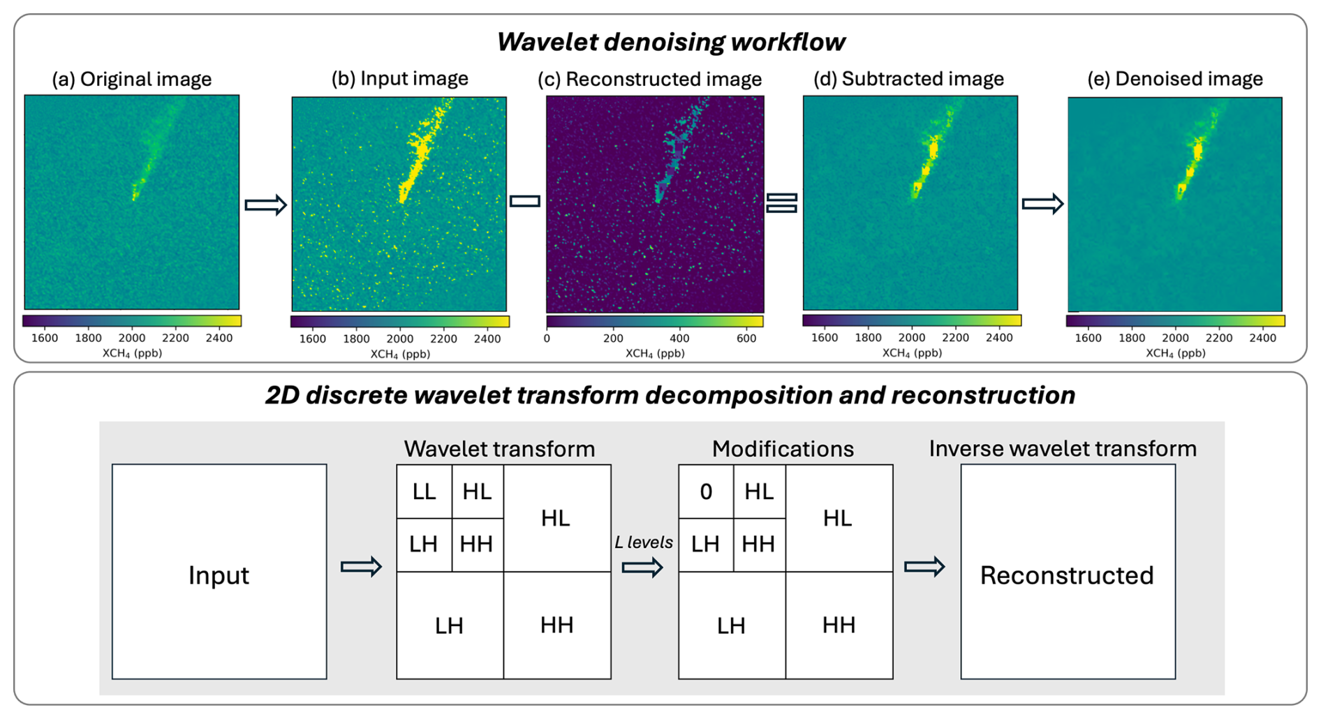
Figure 1 Wavelet denoising workflow. The figure is organized into two rows to distinguish the data processing pipeline from the underlying wavelet transform operations. Top row (left to right): (a) original input image, (b) pre-processed input image, (c) reconstruction from wavelet transform with approximation coefficients removed, (d) residual image obtained by subtracting (c) from (b), and (e) final denoised image after applying soft-thresholding wavelet denoising to (d). Bottom row: illustration of the 2D discrete wavelet transform workflow, showing (i) decomposition into wavelet coefficients, (ii) modification of coefficients by removing the approximation components, and (iii) inverse transform reconstruction used to generate (c).

After this pre-processing, a multilevel 2D discrete wavelet transform is applied to the input image to generate approximation and detail coefficients. The wavelet filter is applied in both horizontal and vertical directions on an image of size m × n , producing four coefficient matrices of size $\frac{m}{\mathrm{2}}$ × $\frac{n}{\mathrm{2}}$ (cA₁, cH₁, cV₁, cD₁), where cA₁ represents the approximation and (cH₁, cV₁, cD₁) represent the details. This decomposition process is repeated recursively on the approximation coefficients, creating additional levels of details, each level capturing finer aspects of the image. The resulting coefficient list includes the approximation coefficients at the Lth level of decomposition and tuples of detail coefficients in descending order of the decomposition level (Eq. 1). We used the Haar wavelet in this step for its simplicity and computational efficiency (Hüpfel et al., 2021; Zanger et al., 2022).

$$\begin{array}{}\text{(1)}& \begin{array}{rl}& \text{Coefficients}\\ & =(c{\mathbf{A}}_L,\left(c{\mathbf{H}}_L,c{\mathbf{V}}_L,c{\mathbf{D}}_L\right),\mathrm{\dots },\left(c{\mathbf{H}}_{\mathrm{2}},c{\mathbf{V}}_{\mathrm{2}},c{\mathbf{D}}_{\mathrm{2}}\right),\\ & \left(c{H}_{\mathrm{1}},c{V}_{\mathrm{1}},c{D}_{\mathrm{1}}\right)),L={\log }_{\mathrm{2}}\left(min(m,n)\right)/\mathrm{2}\end{array}\end{array}$$

After decomposition, a common denoising approach involves setting the detail coefficients to zero and then performing an inverse 2D discrete wavelet transform (Hüpfel et al., 2021). This reconstructs an image of the same size as the input, with the approximation retained and high-frequency details removed. However, this approach causes a loss of detailed plume structure, which is essential for plume visualization. To address this, we followed Hüpfel et al. (2021) and set the approximation coefficients (cA_L) to zero and performed the inverse wavelet transform, building an image that retains only high-frequency components (Fig. 1c). We then subtract this high-frequency image from the input image, so that the resulting image greatly minimizes noise and enhances plumes while maintaining a detailed plume structure (Fig. 1d).

In this process, the decomposition level L is a key parameter. Smaller values of L may retain more high-frequency components, resulting in a large number of false positives. In contrast, larger values tend to over-smooth the data and suppress small methane signals, leading to missed detections (Tables S2 and S12 in the Supplement). To balance these effects, we set L at half of its maximum possible value (Eq. 1).

Finally, we apply soft thresholding wavelet denoising to the processed image for further denoising. This process begins with a wavelet decomposition, followed by shrinking the wavelet coefficients based on their magnitude, such that the coefficients lower than a defined threshold (usually zero) are reduced to the threshold value, while larger coefficients are preserved (Donoho and Johnstone, 1998). As a non-linear filter, it helps suppress small noise-associated coefficients that persists from earlier processing stages, while retaining larger coefficients likely to represent meaningful features. However, this approach may introduce some degree of over-smoothing, particularly for very weak plumes. Once completed, the wavelet coefficients are transformed back to the original domain, producing the final denoised image (Fig. 1e). Note that the pixel values in the denoised image have been subjected to non-linear processing and no longer retain their physical meaning and are therefore unsuitable for flux quantification. Instead, the denoised image is used only for plume masking.

We note that for an ideal linear and orthogonal wavelet transform, the key subtraction step of our denoising method would be equivalent to setting the high-frequency coefficients to zero and reconstructing the image. However, this equivalence does not strictly hold in our implementation due to multiple non-linear steps in this framework, including the pre-processing thresholding, decomposition to a finite level, and the subsequent soft-thresholding of wavelet coefficients. These together result in a structure-preserving denoising rather than a true low-pass filtering.

2.2.3 Mask generation

Based on the denoised image, the plume masks are generated in the following two steps. First, pixels above a threshold value are preserved, where the threshold is defined as the local mean plus a scaling factor (value: 1.5 for MethaneAIR, 1.75 for MethaneSAT) times the local standard deviation (the sensitivity tests of these parameters are discussed in Sect. S1.2). Note that the threshold is determined on the basis of the local background in the denoised image to adapt to spatial heterogeneity caused by surface properties, atmospheric conditions, upwind emitters, and retrieval noise. Second, XCH₄ clumps are identified from these preserved pixels using the 8-connectivity connected component algorithm, which groups adjacent pixels into connected components based on their 8 neighboring pixels (“Queen's” definition). Clumps are then preserved if they exceed a size threshold (100 pixels for MethaneAIR, 500 for MethaneSAT; see their sensitivity analysis in Sect. S1.2). Although binary masks are generated from the denoised image, they are applied to the original concentration map for emissions quantification to conserve mass.

2.2.4 Mask filtering

Given a set of derived plume masks, we filter out false masks by applying specific criteria based on concentrations, plume shapes, and wind direction.

Concentration filtering

The concentration filter aims to remove false masks by finding a high concentration “hotspot” in the original concentration map, a smaller XCH₄ clump with elevated pixel values within the mask. The rationale is that a plume typically features a central hotspot with higher enhancements near the source, diffusing into lower enhancements along the wind direction as the plume spreads out.

The hotspot is defined by a pixel value threshold and a size threshold (10 pixels for MethaneAIR, 20 for MethaneSAT, see their sensitivity analysis in Sect. S1.2). The pixel value threshold is adjustable to the regional background concentration variations resulting from different surface types, weather conditions, etc. (see Sect. S1.1 for details on how these values were adjusted for MethaneAIR and MethaneSAT). We define a hotspot filtering criterion named the hotspot ratio, which is the ratio of the hotspots pixel count to the total pixel count of the mask. Masks with a low hotspot ratio (threshold: 0.002) are discarded, while those with a high hotspot ratio (threshold: 0.03) are accepted without further filtering. Masks with a hotspot ratio in between are further evaluated by the latter filters (this is conceptually similar with Hysteresis Thresholding in Canny, 1986).

Shape filtering

Plumes can take various shapes affected by factors such as flux rate, duration, wind speed and direction, and instrument detection limits. A well-defined plume may appear long and narrow under high winds or in an ellipse or circular shape under low winds. Sometimes the plume may be split into multiple clumps by local eddies, alternating between regions of higher and lower enhancements, resembling several detached bubble-shaped plumes (Fig. S1 in the Supplement). Therefore, in the shape filtering process, we do not restrict our criteria to “standard” plume shapes. Instead, we discard masks with unusual shapes that are clearly not plume-like.

One specific shape to eliminate is the “spider” shape, which consists of multiple branches extending and curling from the center of the mask (Fig. S2). To quantify the degree of curl in such shapes, we introduce the concept of “fiber length”, defined as the length of the longest path along the mask’s skeleton (Fig. S2). For a mask in spider shape, the curling branches lead to a significantly longer fiber length compared to its major axis length (the longest straight line that lies between two boundary points). Based on this observation, we defined a shape filtering criterion by calculating the ratio of fiber length to major axis length, discarding masks with excessively high ratios. The specific parameters used are provided in Tables S7 and S18.

Wind direction filtering

Plumes typically extend along the wind direction, which provides a useful criterion to filter out false masks. To achieve this, meteorological wind data needs to be collected, and the plume origin needs to be identified. In this study, we use High-Resolution Rapid Refresh (HRRR) wind data for U.S. scenes and Global Forecast System (GFS) wind data for all other international scenes. Based on the wind data, the plume origin is determined as the farthest upwind end of the mask. The plume origin from our algorithm is often useful for attribution of plume emissions to particular facilities.

For scenes captured over multiple hours, typically for airborne campaigns, we obtain a range of hourly wind angles from meteorological datasets for the plume origin. Since meteorological data are often coarse both spatially and temporally, we add an angular buffer (55°) to the upper and lower bounds of the wind angle range (its sensitivity is discussed in Tables S6 and S17). For scenes captured at a specific moment, as is often the case with satellite snapshots, we collect a single wind angle and similarly apply angular buffers to get a wind angle range. Finally, we calculate the plume-derived wind angle based on the plume origin and its major axis. Only the plume whose derived wind angle falls within the meteorological wind angle range is preserved. Note that plumes that passed hotspot filtering are not subjected to wind direction filtering, so that high-volume plumes are not removed even if the wind direction in the meteorological product is wrong.

We note that the wind-direction filtering relies on external meteorological data, which may be too coarsely resolved for applications at finer spatial scales or in complex terrain with higher local flow variability and turbulence influence. This may introduce uncertainty in plume alignment and potentially lead to incorrect filtering. Our current wind-direction buffer is relatively wide; however, mismatches may still occur in some cases. Future work could improve upon this by incorporating plume morphology to infer or refine wind direction independently of external meteorological data.

2.2.5 Flux rate quantification

The divergence integral (DI) growing-box method is used to quantify the flux rate of each plume, applying Gauss's theorem through a series of closed surfaces enclosing the source to estimate the flux divergence at increasing distances from the origin. The DI growing-box method has been introduced in Chulakadabba et al. (2023), and here we briefly outline the key steps of implementation. Given a plume origin and the length of the XCH₄ mask, we use the unfiltered XCH₄ map and draw a series of rectangles (“growing boxes”) surrounding the plume origin, with a distance from the origin to the downwind edge of each rectangle ranging from approximately 100 m to the full plume length (up to 10 km). Each successive rectangle is larger than the previous one and completely contains it. The incremental distance between rectangles is one pixel width in each direction, except for the upwind side, where the increment is a quarter of the pixel width. Then based on the measured XCH₄ along each rectangle, we calculate the surface flux divergence integral (kg h⁻¹). The resulting fluxes are then aggregated into a final flux by taking the average over all rectangles that cross the plume. Wind speed and direction from the meteorological product at 80 m height (HRRR or GFS, selected to represent the surface layer windspeed) was used for this calculation, and for sufficiently elongated plumes (eccentricity > 0.87), the wind direction was rotated to match the angle of the major axis of the observed plume.

2.2.6 Validation

Although the proposed wavelet-based plume detection operates without manual input, all plume detections presented in the Results section were also manually validated by independent analysts, including attribution to emitting infrastructure through review of high-resolution satellite imagery and cross-checking against plume detections identified by other methods (Warren et al., 2025).

3 Results

3.1 MethaneAIR results

MethaneAIR campaigns conducted between 2021 and 2023 covered all major oil and gas regions in the United States, accounting for 80 % of the nation's onshore oil and gas production. Warren et al. (2025) provided an in-depth analysis of point source attributions for over 400 methane plumes found across MethaneAIR flights. To identify plumes, they used a gridded application of the DI thresholding method (separate from the DI growing-box method) where the flux divergence was calculated for 600 × 600 m² squares tiled across each scene. Thresholding and clumping were used to find locations with both elevated flux pixels and elevated XCH₄ concentrations. Plumes were then quantified with the same DI growing-box method used in this study. Their analysis found a total flux rate of 360 t h⁻¹ (95 % CI: 285–445 t h⁻¹) from point sources across 13 major US oil and gas basins from flights in 2023.

We applied the wavelet-based plume detection to 46 flights where 338 plumes were previously found by Warren et al. (2025). The wavelet method identified 552 plumes, among which 262 were not previously detected (see Table 1). We used the same DI growing-box method as Warren et al. (2025) to quantify flux rates, allowing for direct quantitative comparison. We observed a small flux difference (within 1-sigma) for most of the plumes found by both methods, suggesting that biases are negligible between the previous DI masking methods and the present wavelet method.

Table 1 Comparison of detection results between the wavelet and DI thresholding methods for 2021–2023 MethaneAIR flights and 24 MethaneSAT scenes. Note that the total number of true detections for MethaneAIR using the DI method is lower than that reported in Warren et al. (2025) due to differences in Level 3 (L3) methane products between dataset versions. The wavelet method used an updated dataset with a reduced spatial domain and additional screening; for consistency, DI detections were restricted to the wavelet processing domain. This affects absolute counts but not the comparative interpretation of method performance.

Most of the plumes detected only by the wavelet method were in lower flux ranges, and the most frequently observed flux rates decreased from 600–1000 kg h⁻¹ in Warren et al. (2025) to 200–600 kg h⁻¹ (Fig. 2). Specifically, among the plumes in the range 200–600 kg h⁻¹ identified by the DI thresholding method, the wavelet method detected 37 out of 53 total (∼ 70 %, while missing the remaining), and added an extra 108; the DI thresholding method detected only 26 % of the wavelet detections. Evidently the wavelet method has a higher sensitivity to “weak” plumes, thus achieves a lower detection limit in MethaneAIR data (Manninen et al., 2026). We present two MethaneAIR plume examples to demonstrate how the wavelet method effectively captures plumes with lower flux rates (Fig. 3). A full list of the 262 additional plumes can be found in the Supplement.

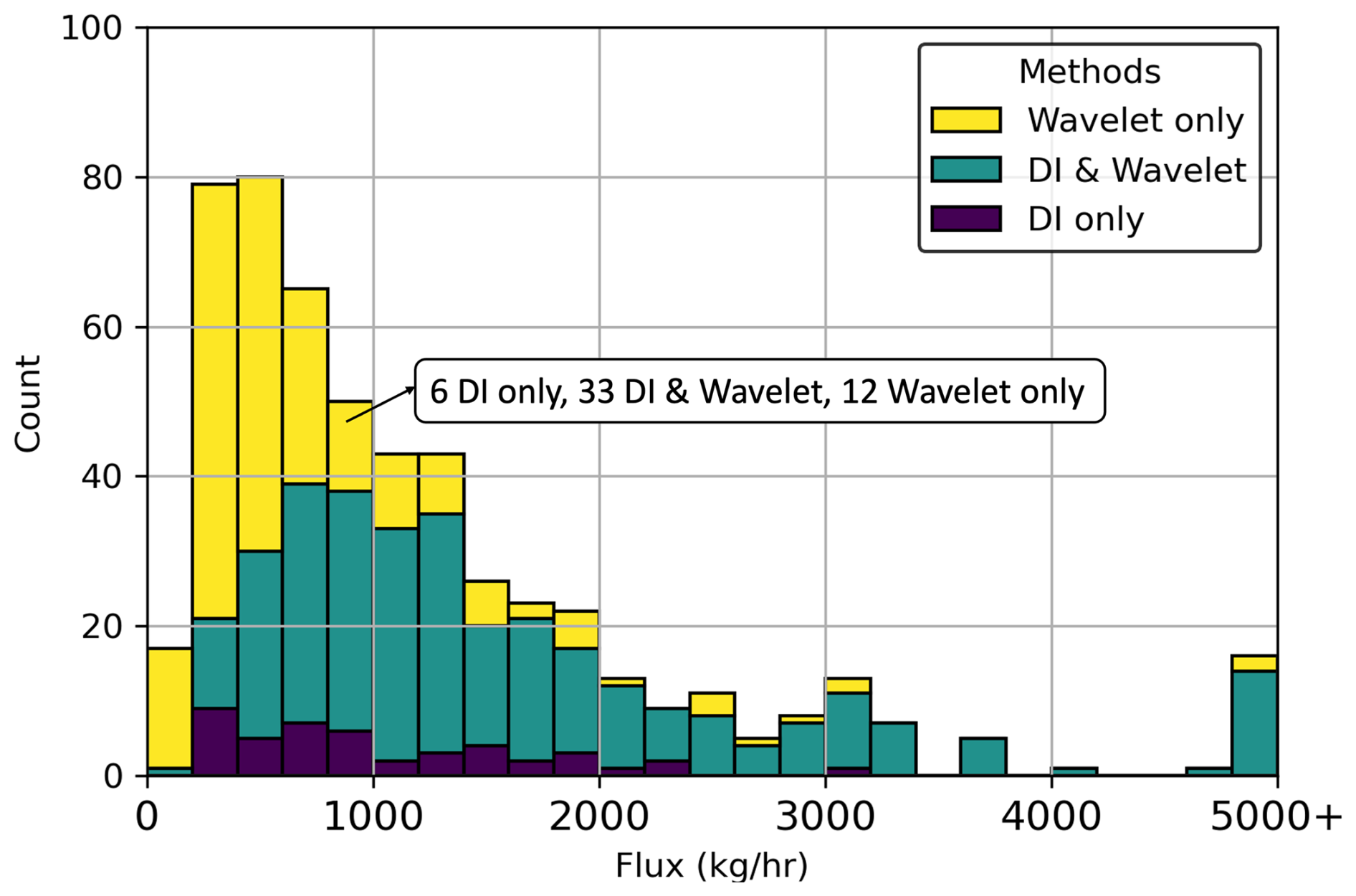
Figure 2 MethaneAIR plumes stacked histogram. Most of the plumes found only by the wavelet method (yellow) lie in lower flux ranges. Most frequently observed flux rates moved from 600–1000 to 200–600 kg h⁻¹ when added with additional plumes found by the wavelet method. The total plume count from two methods is 600.

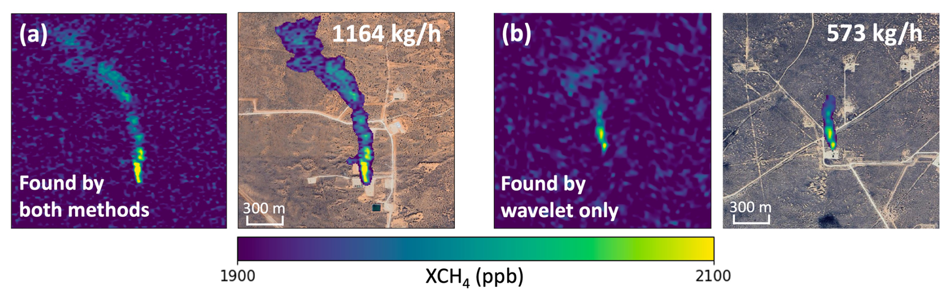
Figure 3 MethaneAIR plume examples (background imagery © 2023 Maxar; map data © 2023 Google). (a) A plume detected by both methods; (b) a low-flux plume detected only by the wavelet method. Plume (b) was not detected by the DI thresholding method as it did not satisfy the joint thresholding criteria requiring both elevated concentration and flux divergence (Warren et al., 2025).

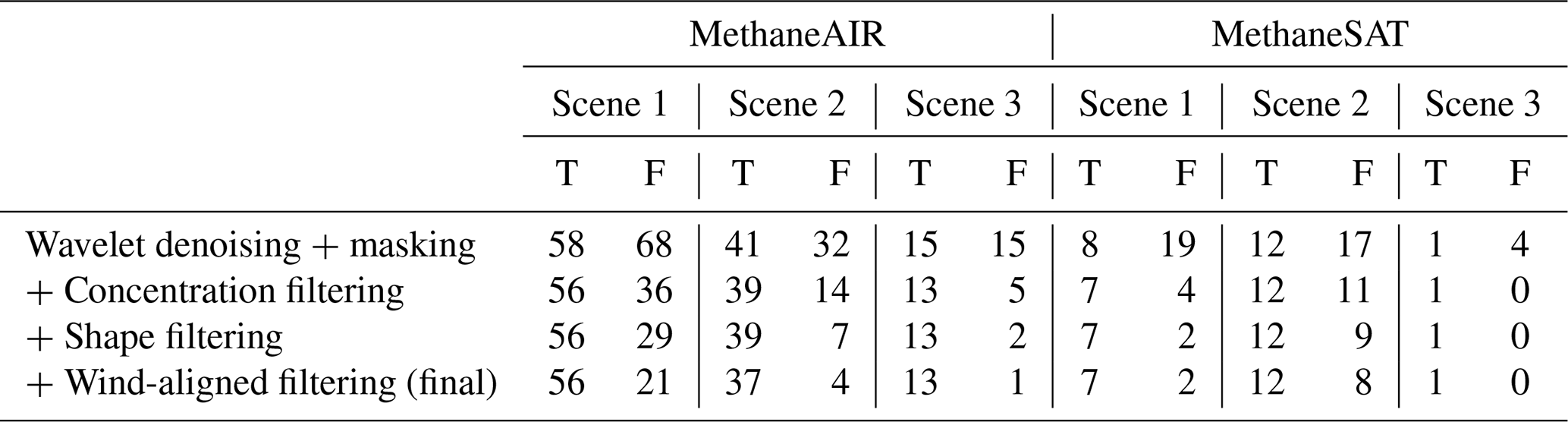
The wavelet method found 181 false positives (FPs) and 48 false negatives (FNs) compared to the DI thresholding method, with significant variations between different flights (FPs were determined by manual inspection, and FNs were determined with reference to DI's true detections). In contrast, the DI thresholding method yielded 919 FPs and 262 FNs compared to the wavelet method. Examining the number of detections at each processing step (Table 2) indicates that the wavelet denoising step determines the initial identification of true plumes, and the subsequent filtering steps, particularly the concentration filtering, play a significant role in reducing false positives. This suggests that the wavelet-based denoising and masking largely control sensitivity, and the filtering steps are critical for improving precision.

Table 2 Cumulative effect of each processing step on true (T) and false (F) detections for three MethaneAIR and three MethaneSAT scenes. Values represent the remaining detections after each step. Scene 1 corresponds to the Permian Basin under high wind conditions, Scene 2 to the Appalachian Basin with low albedo, and Scene 3 to the Permian Basin under low wind conditions.

Background interference differs significantly across these flights, playing an important role in performance. Homogeneity of the background is usually related to the prevalence of nearby emissions, the characteristics of the basin surface, interference by clouds, and instrument differences between campaigns. Notably, background interference accounts for approximately 46 % of false detections. This suggests that background interference remains a major challenge in plume detection; although the wavelet method substantially reduces noise, it does not eliminate it. Future work will therefore focus on developing adaptive, region-specific parameter tuning, for example by using localized metrics that account for spatial variations in background to define more appropriate detection thresholds.

Diffuse enhancements are another important source of FPs, accounting for 42 % of the total. Based on our plume definition in Sect. 2.2.1, enhancements that lack clear hotspot or shape to enable source localization are classified as diffuse enhancements. These could come from dispersed small emissions below the detection limit, intermittent sources that stop emitting before the overpass, or eddies that fragment a plume into detached clumps downwind (Fig. S3b–c). Notably, the DI thresholding method produces approximately three times more diffuse enhancements as false detections compared to the wavelet method, indicating that the wavelet method is more effective at distinguishing source-localizable plumes from dispersed emissions or “inactive plumes”. Diffuse enhancements are particularly challenging for MethaneSAT and MethaneAIR as a result of their high sensitivity and large spatial coverage, with clear signals observed well downwind that would not be detected by many other platforms. Since our method is primarily signal-based, it sometimes struggles to differentiate between true plumes and diffuse enhancements. Although many diffuse emissions were successfully filtered out by concentration filtering and mask size thresholding, some were still identified as plumes. Forthcoming work develops a classifier specifically for diffuse enhancements, using spatial distribution patterns and plume morphology to distinguish them from true plumes and from background. Until this method is fully developed, some level of manual inspection will still be required to achieve a zero-FP dataset.

We next examine the sources of false negatives in the wavelet method. Because no ground-truth dataset is available, this analysis uses detections from the DI thresholding method as a reference. Therefore, our analysis reflects relative rather than absolute performance. In MethaneAIR data, the wavelet method has 48 false negatives, whilst the DI thresholding method has 262. Two primary reasons contribute to missed detections. First, a majority (58 %) of false negatives correspond to relatively weak emissions with limited number of elevated-enhancement pixels (Fig. S4a). In these cases, the wavelet denoising step suppresses the signal by treating it as noise and thus misses the true plume. Second, 24 % of false negatives occur when low-flux emissions coexist with a nearby large plume (Fig. S4b). The presence of the large plume raises the concentration filtering threshold, thus filters out weaker enhancements. Future work will focus on improving sensitivity by adopting less aggressive denoising or applying targeted processing in high-probability regions, and developing adaptive, region-specific parameter tuning to account for local background variability (see more discussion in Sect. 4.3).

In addition, we also observe rarer but more challenging cases where plumes merge and multiple plumes are grouped within the same mask (Fig. S5a). In this case, we tend to treat the combined plume as a single source and quantify the total emissions from both sources together. Addressing this issue may involve analyzing the hotspot locations, the distance between masks, and the wind direction. Furthermore, some false negatives arise because the wavelet method was applied to updated concentration maps with additional screening process (Fig. S4c). In this situation, partial removal of plume pixels results in fragmented plumes that are more difficult to identify.

3.2 MethaneSAT results

With its high spectral resolution (0.24 nm) and large swath width (200 km), MethaneSAT provided clear signals of emissions not only near the source but also a significant distance downwind. However, these capabilities also introduce new challenges for plume detection, as not all emissions can be directly attributed to specific point sources or reliably quantified. Its coarser spatial resolution relative to point source imagers also makes it more difficult to differentiate spatially proximate point sources.

We applied both the wavelet and the DI thresholding methods to 24 MethaneSAT scenes in 2024–2025 and compared results (Table 1 and Fig. 4). The wavelet method achieved an equal or higher number of true detections and a lower number of FPs in most scenes (again, FPs were determined by manual inspection). In some cases, the improvement of true detections (scene 2) and the reduction of FPs (scene 6) is significant. This is consistent with what we observed in MethaneAIR data, indicating that the higher sensitivity of this method to “weak” plumes generally holds true across different platforms. Figure 5 offers a similar quantification comparison to what we did with MethaneAIR, where we again observed a higher contribution of the wavelet method to low-volume emissions. The most frequently observed flux rates lay in the range of 2–3 t h⁻¹, although we probably missed data in the range 3–7 t h⁻¹ due to the small sample size.

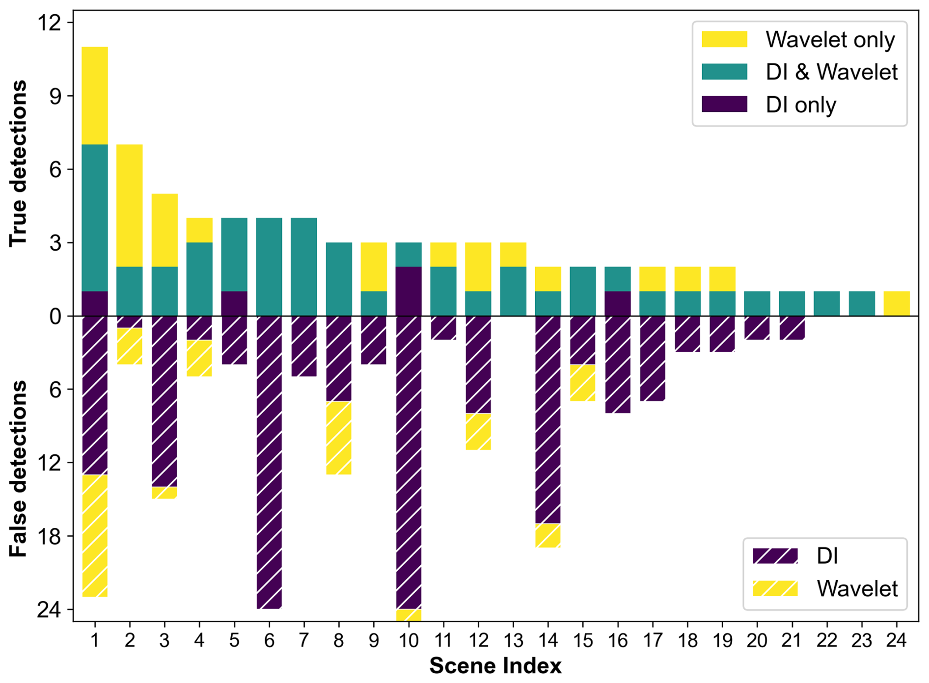
Figure 4 Detection performance of the wavelet and DI thresholding methods on MethaneSAT scenes. Compared to the DI thresholding method, the wavelet method generally found a higher number of true detections and a lower number of false detections. The true detection stacked bars are additive, whilst the false detection stacked bars are selective.

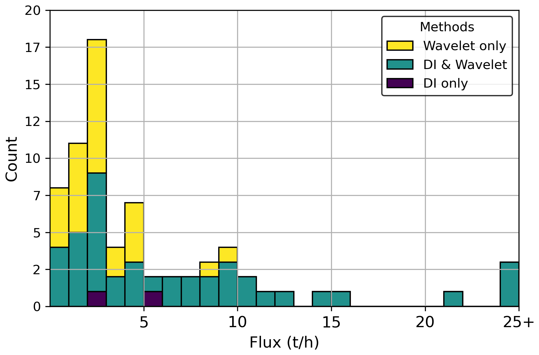
Figure 5 Plumes stacked histogram across 24 MethaneSAT scenes. Similar with MethaneAIR, most of the plumes found only by the wavelet method (yellow) are in lower flux ranges.

Figure 6 presents a MethaneSAT XCH₄ image with plumes segmented using the wavelet and DI thresholding methods. Compared with MethaneAIR, MethaneSAT captured significantly longer downwind plume tails, portions of which extended beyond the wavelet mask boundaries. We did not expand the plume masks farther downwind, as doing so would require lowering the plume-detection thresholds, which increases the probability of more false detections. In addition, restricting the masks to the plume segment within 5–10 km of the source generally produces more accurate flux estimates, because expanding the masks farther downwind increases the chance of including nearby sources in the DI growing boxes, thereby biasing flux calculations. Expanding the masks can also increase violations of the steady-wind assumption due to spatial and temporal wind variability. Averaging the fluxes from growing boxes spanning 5–10 km still provides sufficient data for a robust average flux estimate.

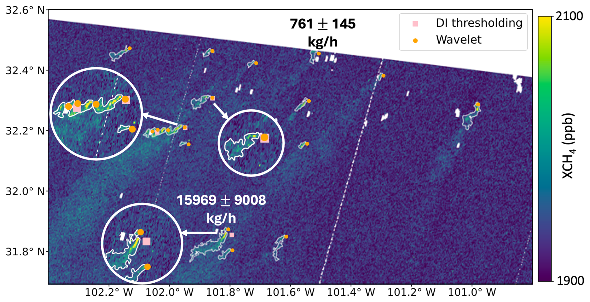
Figure 6 MethaneSAT plume examples. Both the DI thresholding method and the wavelet method found 4 plumes (the zoomed-in view), and the wavelet method found additional 13 plumes. Flux rates range between 1 and 10 t h⁻¹, with the lowest and highest marked adjacent to the plume sources.

We generally found more false detections for MethaneSAT than MethaneAIR using both the wavelet and DI thresholding methods, primarily because the high sensitivity of MethaneSAT led to more frequently observed diffuse enhancements, which account for 65 % of the total false positives (Fig. S6). This is largely due to its ability to capture long plume tails (on the order of tens of kilometers), which, under complex wind conditions, can fragment into spatially dispersed enhancements that are difficult to trace back to a single source. In addition, the broader spatial coverage and higher signal-to-noise sensitivity of MethaneSAT make it more likely to detect intermittent emissions, further increasing the occurrence of diffuse enhancements.

In addition, the wavelet method achieved a much lower false negative rate in the MethaneSAT dataset, missing only 2 plumes detected by the DI thresholding method. Similar to the findings in the MethaneAIR analysis, both missed plumes coexist with a large plume in the same scene, where the elevated concentration threshold caused by the larger plume filters out weaker enhancements (Fig. S7). These observations suggest a need to improve the concentration filtering approach to better account for diffuse plumes and local background conditions in MethaneSAT observations.

Another challenge that occurred more often on MethaneSAT is the presence of overlapping plumes. Because MethaneSAT captured longer plume tails, the downwind ends of the plumes in proximity are more likely to overlap (Fig. S5b). This increased the difficulty of quantification as it required manual adjustment of the plume length. Potential ways to address this problem are to explore plume segmentation techniques.

4 Discussion

4.1 Comparison with alternative methods

To better contextualize the performance of the proposed wavelet method, we conducted additional analyses comparing (1) the denoising strategy, (2) the choice of wavelet basis, and (3) computational efficiency relative to other commonly used approaches.

4.1.1 Comparison with conventional denoising methods

We first evaluated the impact of the denoising step by comparing the wavelet denoising step with two alternatives: Gaussian filtering and median filtering. Gaussian filtering used a 2D isotropic Gaussian filter with standard deviation of 3 pixels, and median filtering used a 3 × 3 pixel moving window. We directly replaced the wavelet denoising step with these methods while keeping all subsequent filtering steps identical. The comparison was performed across three MethaneAIR scenes and three MethaneSAT scenes spanning a range of background and wind conditions, consistent with what we used in the sensitivity analysis.

The results (Tables S8 and S19) show that our approach consistently yields a higher number of true detections compared to both Gaussian and median filtering. In addition, the alternative methods produce either comparable or higher numbers of false detections in most of the scenes. This indicates that while conventional denoising techniques can suppress noise, they are less effective at preserving plume structures across spatial scales, leading to reduced detection sensitivity.

4.1.2 Sensitivity to wavelet choice

Next, we assessed the sensitivity of the results to the choice of wavelet by testing several commonly used families, including Daubechies (db4), Symlets (sym4), and biorthogonal wavelets (bior4.4). These wavelets represent different mathematical properties, such as compact support (db4), increased symmetry (sym4), and linear phase reconstruction (bior4.4) (Mallat, 1999).

As summarized in Tables S9 and S20, we do not observe a significant difference between the Haar wavelet and the alternative wavelets in terms of the number of true and false detections. In most cases, the other wavelets yield equal or fewer true detections and equal or more false detections. Furthermore, the plume masks generated using the Haar wavelet are generally similar to, and in some cases more physically reasonable than, those produced by the other wavelets (Fig. S8). These findings support the use of the Haar wavelet as a simple and effective choice for this application. We note that continuous wavelet transforms are not considered here, as they do not naturally integrate into the reconstruction-based denoising framework used in this study.

The sensitivity analysis to the other parameters can be found in Sect. S1.2. We note that in this study, the parameter selection was guided by maximizing plume detections while minimizing false positives, which may introduce the risk of overfitting to specific datasets and observing conditions. Although the chosen parameters show consistent performance across multiple scenes, their optimal values may vary under different environmental and instrumental conditions. Future work can focus on evaluating the generalizability of these parameters using larger and more diverse datasets, and on developing adaptive or region-specific tuning strategies (see Sect. 4.3).

4.1.3 Computation efficiency

Furthermore, we compared the computational efficiency of the wavelet method with the DI thresholding method and a representative ML method (see more information in Sect. S1.3). Table S21 reports the total runtime and peak memory usage required to process a single scene, averaged over the same set of observations. The wavelet method does not provide an advantage over the DI method in terms of runtime or memory usage. However, because it does not require training data or a training stage, the wavelet method is still substantially more efficient than the ML-based approach.

We note that the reported values reflect only the cost of applying the optimized methods and do not include parameter tuning. In the wavelet method, the computational cost of parameter tuning scales approximately linearly with the number of parameter combinations tested.

4.2 Probability of detection

To further quantify detection limits and evaluate algorithm performance across a broader range of conditions, we refer to a companion study by Manninen et al. (2026).

In that work, a probability of detection (P_d) framework is developed to compare plume detection performance across different observing systems (including MethaneAIR and MethaneSAT) and detection algorithms (including the wavelet method and the DI thresholding method). The framework uses a nondimensional “observability” predictor that combines emission rate, wind speed, pixel size, and gas concentration noise, and maps it to detection probability using logistic regression (here observability = $\log \left(\frac{q}{\sqrt{a}nu}\right)$, q = emission rate per unit area, a = pixel area, n = noise amplitude, u = windspeed). The analysis is based on ∼ 80 000 synthetic plumes generated using Weather Research and Forecasting Large Eddy Simulations (WRF-LES), spanning a wide range of atmospheric conditions and noise characteristics, as well as ∼ 62 000 scenes derived from controlled-release experiments using image processing methods (Chulakadabba et al., 2023; El Abbadi et al., 2024).

Results show that the wavelet method generally outperformed the DI thresholding method by finding more plumes and more low emission rate plumes. It is also more robust to real-world satellite scenes with missing data. A comparison of P_d between the two methods across different observability conditions is provided in Fig. S9. Overall, the wavelet method shows lower P_d than DI thresholding at very low observability, likely due to the suppression of weak plumes near the detection limit during multi-scale feature extraction and thresholding. However, its performance surpasses DI thresholding at moderate to high observability, reflecting its stronger ability to enhance plume structures and suppress noise, which leads to more reliable detections.

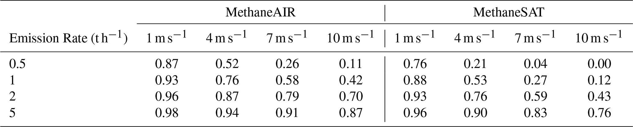
Manninen et al. (2026) also quantified differences in plume detection capability across observing systems. The wavelet method achieves a P_d of 0.93 and 0.42 at wind speeds of 1 and 10 m s⁻¹ for emissions of 1000 kg h⁻¹ in MethaneAIR. For MethaneSAT, it achieves a P_d of 0.93 and 0.43 under the same wind conditions for emissions of 2000 kg h⁻¹. A summary of detection probabilities across different emission rates and wind speeds is provided in Table 3.

Table 3 Probability of detection (P_d) for the wavelet method under different emission rates and wind speeds for MethaneAIR and MethaneSAT.

We note that this analysis evaluates the performance of the full detection and masking framework, and does not explicitly isolate the effect of individual processing steps. Introduction of frameworks using many different denoising approaches and conditioning/filtering would be required for systematic evaluation of each step, including the effects of hyperparameter choices and noise characteristics, which lies beyond the scope of this paper.

4.3 Future work

We have applied the wavelet method to the whole scene with no prior information of point source locations. Looking ahead, we plan to further improve its sensitivity to plumes by applying targeted wavelet denoising to subregions where plumes have been identified in previous top-down observations, or where known oil and gas infrastructure exists. This could include a growing dataset of past observed plume locations by MethaneAIR and MethaneSAT, as well as integration with external datasets such as the methane point source database from the International Methane Emissions Observatory (IMEO) (UNEP-IMEO, 2023), and the Oil and Gas Infrastructure Mapping database (OGIM) (Omara et al., 2023). It would allow the use of lower detection thresholds in high-probability emission areas, so that we can capture weaker plumes that may be missed in full-scene processing. It also reduces false positives due to lower background heterogeneity within subregions.

The current concentration filtering step does not fully address diffuse enhancements and can be influenced by the presence of high-emission plumes. Future improvements will explore adaptive and region-specific threshold tuning. For example, a localized metric similar to the “observability” defined by Manninen et al. (2026) could be used to determine pixel-level thresholds within each subregion. This metric would account for spatial variability in background heterogeneity, noise characteristics, and wind conditions, enabling more consistent performance across diverse scenes.

Additionally, false detection classifiers targeting specific artifact types can be developed and integrated into the plume detection models. For example, albedo artifacts and diffuse enhancements may be classified based on the spatial patterns of surface reflectance and methane concentration, as well as plume morphology and wind alignment. Incorporating these features into a post-processing classification step could reduce false detections while allowing more permissive plume-identification thresholds, thus improve overall detection sensitivity without sacrificing reliability.

Our method is based on feature extraction and signal-vs.-background separation, which do not rely on any physical or chemical properties of methane. Given that it targets generic characteristics of point-source plumes, this method is designed to be readily adaptable to different observing systems for any trace gases that exhibits plumes from discrete emitters. These extensions would require validation and parameter tuning, thus are beyond the scope of this study.

5 Conclusions

In this study, we propose a new automated methane plume masking method that uses atmospheric methane concentration data with no prior knowledge of source locations, to find plumes, determine plume origins, and create binary masks. This method uses a 2D discrete wavelet transform, a technique typically used in image processing, to enhance plumes and reduce background noise in XCH₄ imagery, combined with advanced filtering of detected plumes. It significantly improves the effectiveness of thresholding compared to current methods for methane plumes by more precise separation between plume and background signals. We demonstrate the performance of this method using both airborne data from MethaneAIR and spaceborne data from MethaneSAT. Across these platforms, the wavelet method consistently performed with higher sensitivity to weak plumes that are more often missed by conventional techniques.

Background interference and diffuse enhancements continue to drive a large fraction of false detections, while weak or small plumes and those coexisting with strong emissions contribute to missed detections. These limitations arise from spatial variability in background conditions and the use of uniform denoising and thresholding strategies. Future improvements will focus on targeted processing in high-probability regions to improve sensitivity, adaptive and region-specific parameterization to account for background variability, and the development of artifact-specific classifiers to distinguish diffuse enhancements and other artifacts from true plumes.

Although our algorithm does not entirely eliminate false detections, it achieves a lower false positive rate than basic thresholding methods by reducing background noise, which reduces the requirements for manual inspection. Additionally, it has a lower computational cost than machine learning models as it needs no labeled training data or model training phase. This algorithm is designed to be readily adaptable to a wide range of aircraft and satellite platforms and use cases for methane and other trace gases exhibiting plume-like structures in both research and operational contexts.