Combined and autonomous online measurement of water isotopes in snowflakes and atmospheric water vapor in East Antarctica

Water isotopes in precipitation are a powerful tool to better understand the processes governing snowfall in Antarctica, which is essential to improve our knowledge of the Antarctic atmospheric water cycle and surface mass balance, and for the interpretation of past climate signals archived in ice cores. However, precipitation isotope observations in Antarctica rely on manual sampling, which is prone to fractionation under low accumulation rates and remains both time-consuming and logistically demanding, and thus restricted to stations and seasons where manual sampling is feasible.

In this study, we present a novel method that enables autonomous, continuous, and combined measurements of water vapor and precipitation δD, using a single laser spectrometer. This technique offers new observational capabilities to better capture the isotopic signature of snowfall events in polar environments. Compared to conventional manual sampling of precipitation, the technique is capable of analysing very small amounts of water, while avoiding post-depositional effects. In addition, it enables high-temporal-resolution observations and is well suited for long-term deployments in unmanned environments. The sampling system prototype has been deployed at Dumont d'Urville station, located on the coastal margin of East Antarctica, and evaluated during three precipitation events from February to June 2023. A dedicated post-processing algorithm was developed to retrieve the isotopic composition of precipitation from the surrounding vapor background. Comparisons with independently collected snow samples show a mean deviation of −5.4 ‰ in δD, which is well below the observed intra-event signal amplitude of about 100 ‰. This demonstrates the reliability of both the sampling system and the retrieval algorithm to study the isotopic composition of precipitation at the event-scale. With this new dataset, two approaches are proposed to better understand the water vapor – precipitation relationship at Dumont d'Urville: (1) an evaluation of the LMDZ6iso general circulation model, and (2) a comparison with ground-based remote sensing instruments (ceilometer and micro rain radar) to explore the link between the Δ(δD) metric and the vertical structure of precipitation. Beyond polar applications, the proposed method opens new possibilities for other types of observations, including liquid precipitation sampling or cloud water isotopes monitoring onboard aircraft.

1 Introduction

Water isotopes are largely used for documenting the climate and water cycle since the early studies of Dansgaard in the 1950's (Dansgaard, 1954). The isotopic composition of water has been analysed in precipitation (Ehhalt et al., 1963), snow (Gonfiantini and Picciotto, 1959; Lorius, 1961) and ice (Dansgaard et al., 1960). The isotopic ratio in precipitations can be linked to the temperature at high latitudes and to the quantity of precipitation (amount effect) at low latitudes (Dansgaard, 1964). The isotopic composition of water in precipitation can also provide constraints on the origin or climate conditions of the evaporative regions (Jouzel et al., 2013), moist air trajectories and mixing of water masses (Jouzel et al., 2013; Rozanski et al., 1982), and mean temperature in clouds, where snow is formed (Picciotto et al., 1960).

More recently, advances in laser spectroscopy have made possible continuous measurements of the isotopic composition of water vapor by instruments at ground or near ground level in several monitoring sites, with some observations lasting for several years (González et al., 2016; Guilpart et al., 2017; Leroy-Dos Santos et al., 2021, 2023; Noone et al., 2011; Steen-Larsen et al., 2013; Worden et al., 2007). The water vapor isotopic composition integrates the effect of phase changes along the atmospheric water cycle, thus providing added value for the understanding of the related processes. With these continuous vapor measurements, it is now possible to better identify effects such as evaporation over the ocean (Bonne et al., 2019), mixing of several air masses or re-evaporation (Landais et al., 2024), or exchange at the interface between snow and atmosphere (Steen-Larsen et al., 2013; Wahl et al., 2021).

In parallel with the increasing number of observations of the isotopic composition of water vapor and precipitation, several atmospheric general circulation models were equipped with water stable isotopes (Risi et al., 2010; Schmidt et al., 2007; Werner et al., 2011). Adding water isotopes to the models allows for the testing and improvement of the representation of the atmospheric water cycle. Pairing isotopic composition of water vapor and precipitations is also a strong added value for studying processes such as below cloud evaporation or mixing of air masses (Dütsch et al., 2016; Graf et al., 2019; Xing et al., 2023), while the additional use of cloud water isotopic measurement (Lowenthal et al., 2016, 2011) opens new insights into cloud processes (snow formation, riming, water vapor deposition). When coupled with remote sensing techniques, water isotopes can become powerful tools to improve our understanding of cloud microphysical processes (Muller et al., 2015; Weng et al., 2021).

Water isotopes are largely used in polar regions because their measurements in ice cores enable reconstructing the past temperature as well as patterns of the atmospheric water cycle. In Antarctica the longest continuous record of water isotopic composition was obtained on the EPICA Dome C ice core drilled at Concordia station (Jouzel et al., 2007). This record covers the last 800 000 years and depicts the climate variability on the orbital timescale (glacial – interglacial cycles lasting between 40 000 and 120 000 years), millennial timescale (Antarctic Isotopic Maxima during glacial periods) down to multi-decadal timescale (Grisart et al., 2022; Pol et al., 2014). Ice core recovery in more coastal regions with higher accumulation rate also permits to provide reconstructions at an annual scale (Emanuelsson et al., 2022; Jones et al., 2023).

The interpretation of the ice core records in Antarctica benefits more and more from water isotope enabled atmospheric general circulation models which can be evaluated using the isotopic composition of both precipitation and water vapor available at some stations (Bagheri Dastgerdi et al., 2021; Dutrievoz et al., 2025; Leroy-Dos Santos et al., 2023; Ollivier et al., 2025b). The relatively good agreement observed between modelled vapor and observations from the few equipped stations provides confidence in the model skills. Still, discrepancies remain, and in particular there is to our knowledge no study in which both water vapor and precipitation isotopic composition are well reproduced by the model outputs. Such mismatch is a limitation for the interpretation of water isotopic records in snow and ice in Antarctica.

Several explanations can be provided for the mismatch in the precipitation isotopic composition which can be linked to the representation or parameterization of the physical processes during precipitation formation and snow particle fall through the atmospheric column in polar region or simply to side effects of the sampling after a precipitation event. Indeed, under the influence of surface radiation and surface wind, the snow isotopic composition after a snowfall event can be rapidly obliterated by sublimation or metamorphism. This is the reason why samples are regularly discarded from the series of precipitation isotopic composition at Concordia because their anomalous isotopic values cast doubt on possible influence of post-deposition sublimation after the snowflake deposition on the sampling tables (Dreossi et al., 2024; Ollivier et al., 2025a).

We aim here at better describing the relationship between the isotopic composition of precipitation and the isotopic composition of water vapor and associated processes by getting rid of any influence of post-deposition processes between the snowfall event and the precipitation sampling. We thus present a new method enabling online measurements of the isotopic composition of falling snow near ground level in parallel to continuous isotopic measurements of the surrounding water vapor. We first present the instrumental setup deployed at the Dumont d'Urville (DDU) station as well as the calculation for recovering the snowflake isotopic composition (Sect. 2). We then focus on a few precipitation events at DDU station to evaluate the accuracy of the new method (Sect. 3). Finally, we discuss the strengths and limitations of this new method and illustrate its potential to improve our understanding of the processes controlling the isotopic composition of precipitation in conjunction for instance with the use of general circulation model equipped with water isotopes or ground-based remote sensing observations (Sect. 4).

2 Methodology

2.1 Site description

The Dumont d'Urville Station (DDU) is located in Adélie Land, at 66°400 S, 140°010 E, on a small island approximately 1 km off the Antarctic coast. Since 2018, atmospheric water vapor isotopes have been continuously monitored at DDU using a Picarro L2130-i cavity ring-down spectrometer (Leroy-Dos Santos et al., 2021), with typical humidity and δD values reported in Table 1 from Leroy-Dos Santos et al. (2023). During the austral summer season 2022–2023, the instrument was relocated to a new laboratory dedicated to atmospheric observations (hereafter referred to as the ATMOS building). At the same time, a ProCEAS analyzer (AP2E) laser spectrometer, based on the recently developed cavity enhanced absorption spectroscopy technology, was installed (Lauwers et al., 2025). The ATMOS building is situated on the southern part of the island, facing the prevailing wind direction, to reduce contamination from station buildings and activities.

In addition to water isotope measurements, standard meteorological parameters are recorded by a Météo-France weather station located close to the ATMOS building. These measurements include temperature, wind speed and wind direction reported in Table 1 and cover the period from December 2022 to August 2023. Furthermore, two remote sensing instruments complement the in-situ observations: a ceilometer (CL31, Vaisala), which provides continuous measurements of cloud base height, and a micro rain radar (MRR2, Metek) (Grazioli et al., 2017), which enables vertical profiling of precipitation (radar reflectivity) from the surface up to 3 km.

Table 1 Meteorological data from the Météo-France weather station, including mean temperature, wind direction, wind speed, and absolute humidity. The observation period includes winter 2022–2023 (DJF), summer 2023 (JJA), and the three case studies. For the case studies, the number of collcted snow samples (collected in the tray or in the wind sock, see Sect. 2.3) and the duration is also reported, where the start (resp. end) corresponds to the first (resp. last) collected snow sample.

2.2 Water isotopes instrumental set-up

The instrumental setup includes the Picarro L2130-i, which continuously monitors atmospheric water vapor isotopic composition, and the ProCEAS analyzer (AP2E). The latter was specifically implemented to test the feasibility of the combined, autonomous online measurement of both atmospheric water vapor and precipitation isotopic composition. The calibration of the water isotopes analysers are performed with an updated version of the low-humidity level generator (LHLG) (Lauwers et al., 2025; Leroy-Dos Santos et al., 2021) installed during the summer season 2022–2023. A new sampling line was also installed on the ATMOS building during the same field campaign to capture snowflakes, as well as four additional electrovalves (V3 to V6) controlled by the LHLG software with a sequencer (Fig. 1).

Figure 1 Sampling system. Left: photo of the 3 m sampling line installed on the ATMOS roof, showing the water vapor inlet (downward-facing, with a filter) and the snowflake inlet (upward-facing, $\mathrm{1}/\mathrm{8}$ in. aperture). The location of Dumont d'Urville Station (DDU) is indicated in the upper-left panel. Right: schematic of the full setup, including the external inlets, heated tubing, electrovalve system, calibration unit, and AP2E/Picarro laser spectrometers.

The 3 m sampling lines consists of two PFA tubes and a heating cord enclosed in an insulated sleeve, running from the roof of the ATMOS lab to the instruments inside. The first inlet (“water vapor inlet”) is oriented downward and protected with a sintered filter (stainless steel, 16 mm diameter) and cap to prevent snow intrusion. It is continuously flushed at 10 L min⁻¹ by a KNF N96 pump and connected to both the Picarro and AP2E analysers for ambient water vapor measurements. The second inlet (“snowflake inlet”) is oriented upward with a small aperture ($\mathrm{1}/\mathrm{8}$ in.) to allow snowflakes collection in addition to water vapor. Inside the heated tube, incoming snow particles are sublimated, and the vapor is drawn into the AP2E analyser. The four electrovalves, alternate between three operating states (Table 2). In the “Air” state, both analysers measure ambient vapor while both inlets are flushed at 10 L min⁻¹. Every 45 min, the system switches to the “Flake” state for 15 min: the Picarro instrument continues measuring ambient vapor, while the AP2E instrument is connected to the snowflake inlet, now carrying a mix of ambient vapor and sublimated snow. During this period, electrovalve V6 stops flushing the snowflake line so that 100 % of the sublimated sample enters the analyser. Finally, every 46 h, a calibration with two reference water isotopic standards is performed with the LHLG and lasts approx. 2 h.

Table 2 Description of the three operating states of the system (“Air,” “Flake,” “Calibration”), including the electrovalve configuration and typical frequency. The ports labels for V6 are shown in Fig. 1.

This configuration allows uninterrupted water vapor time series from the Picarro, while enabling the AP2E to measure precipitation and vapor in parallel. It should be noted that the present set-up does not allow discrimination between different types of ice particles (e.g., snowfall, drifting or blowing snow). Additional observations are required to disentangle these contributions on a physical basis, such as based on wind speed and direction, snow particle counters, snow imaging systems (to characterize particle shape and type), and remote sensing instruments (radars, lidars).

2.3 Snow sample collection and measurement

During precipitation events throughout the year, snow is collected by overwintering staff at high temporal resolution using two complementary methods: a wind sock mounted on a wind vane, which is able to capture snow associated with horizontal winds, and a 50 cm-deep tray which will preferentially collect vertically falling snow (Fig. 2). At the onset of each event, both collection devices are emptied to avoid contamination from previous snow accumulation. The collected snow is then transferred into 50 mL Corning tubes, with a sampling period varying between 1 to 3 h depending on the snowfall rate. To prevent mixing of snow over long periods and limit post-depositional processes such as sublimation, no sample was collected if the snow volume remained insufficient after three hours. The collection device location was constrained by logistical requirements (easy access during harsh winter conditions) but oriented toward the dominant wind direction (south-east), minimizing potential shielding by nearby building. This particular high-resolution sampling has been performed on a few events in 2023 to validate this study. The selection of events was based on practical criteria (availability of the overwintering staff) and meteorological conditions. The overwintering staff ensured that continuous manual sampling could be performed without interruption when forecasts indicated precipitation lasting more than 24 h, in order to obtain a few long and high-resolution datasets. Outside of these events, manual sampling was performed only during standard working hours. Samples were stored at −20 °C at the station, then shipped to LSCE in refrigerated containers during the following austral summer.

Figure 2 Manual snow collection setup (1 m above ground level). Left: sock mounted on a wind vane, designed to collect blowing snow. Right: open tray, preferentially capturing vertically falling snow.

The isotopic measurements were conducted at LSCE using a Picarro L2130-i spectrometer in liquid mode. The standard deviation of δD measurements (1σ) was 0.7 ‰, estimated from duplicate measurements on 15 % of the samples (δ¹⁸O measurements are not presented in this study; the reasons for this choice are detailed in the next section).

2.4 Water vapor isotopic composition correction

At DDU, the minimal ambient humidity is around 500 ppm (Leroy-Dos Santos et al., 2023), while maximal values can exceed 10 000 ppm in our setup, especially in the “snowflake inlet”, when snowflake sublimation adds substantial water vapor. Current AP2E water isotope analysers are not optimized for such high humidity levels, as excessive optical absorption under these conditions can cause non-linearities. This “saturation” effect is particularly pronounced for δ¹⁸O, requiring specific spectral fitting procedures (Piel et al., 2024), while its impact on δD remains limited (Lauwers et al., 2025). Consequently, this study focuses on δD only.

Two main corrections are applied to the raw isotopic ratios given by the two spectrometers, already described in previous papers (Lauwers et al., 2025; Ollivier et al., 2025b):

• humidity dependency correction: a linear correction is accounted for the AP2E instrument (Lauwers et al., 2025). For the Picarro instrument, we account for a typical humidity dependency in the form of $f\left(h\right)=a_{\mathrm{1}}/h+b_{\mathrm{1}}h+c_{\mathrm{1}}$ (Weng et al., 2020), where h is the absolute humidity (in ppm). The reference humidity is fixed at 1000 ppm, for which the correction function is equal to 0. The corrected δD value reads $\mathit{\delta }{\mathrm{D}}_{\text{humcorr}}=\mathit{\delta }{\mathrm{D}}_{\text{raw}}-f\left(h\right)$. The parameters retrieved from the calibration are summed-up in Table 3.

• true value correction: correction parameters are retrieved from regular calibration data acquired during year 2023 at DDU with two VSMOW-SLAP calibrated standards FP5 ($\mathit{\delta }\mathrm{D}=-\mathrm{394.7}$ ‰ ± −0.7 ‰) and AO1 ($\mathit{\delta }\mathrm{D}=-\mathrm{238.3}$ ‰ ± −0.7 ‰), at a reference humidity of 1000 ppm. The true value correction reads $\mathit{\delta }{\mathrm{D}}_{\text{true}}=a_{\mathrm{2}}\cdot d{\mathrm{D}}_{\text{humcorr}}+b_{\mathrm{2}}$, where δD_humcorr is the isotopic composition corrected from the humidity dependency. The true value correction parameters are given in Table 2.

Table 3 Humidity dependency and true value correction parameters for both AP2E and Picarro spectrometers.

2.5 Retrieval of the isotopic composition of precipitation

Let us assume atmospheric water vapor of absolute humidity h_v(t) and isotopic composition δ_v(t) (in oxygen 18 or deuterium), hereafter denoted “background water vapor”. When a snowflake sublimates, its isotopic composition δ_p is diluted in the surrounding water vapor, resulting in a mixing between the snow sample and the background, with a total humidity h_mix(t) and isotopic composition δ_mix(t).

To reconstruct the isotopic composition of the sublimated snow sample δ_p, we apply the formulation proposed by Affolter et al. (2014) for calculating the isotopic composition of liquid water inclusions in speleothems:

$$\begin{array}{}\text{(1)}& {\mathit{\delta }}_{\mathrm{p}}={\displaystyle \frac{\stackrel{\mathrm{‾}}{{\mathit{\delta }}_{\text{mix}}}\stackrel{\mathrm{‾}}{h_{\text{mix}}}-\stackrel{\mathrm{‾}}{{\mathit{\delta }}_{\mathrm{v}}}\stackrel{\mathrm{‾}}{h_{\mathrm{v}}}}{\stackrel{\mathrm{‾}}{h_{\text{mix}}}-\stackrel{\mathrm{‾}}{h_{\mathrm{v}}}}}={\displaystyle \frac{\stackrel{\mathrm{‾}}{{\mathit{\delta }}_{\text{mix}}}\stackrel{\mathrm{‾}}{h_{\text{mix}}}-\stackrel{\mathrm{‾}}{{\mathit{\delta }}_{\mathrm{v}}}\stackrel{\mathrm{‾}}{h_{\mathrm{v}}}}{h_{\mathrm{p}}}}\end{array}$$

Here the horizontal bar denotes the integrated value across time of both the humidity and the isotopic composition, the latter being weighted by the humidity value. Their values are calculated as follow:

$$\begin{array}{}\text{(2)}& \stackrel{\mathrm{‾}}{{\mathit{\delta }}_j}={\displaystyle \frac{\int {\mathit{\delta }}_j\left(t\right)h_j\left(t\right)\mathrm{d}t}{\int h_j\left(t\right)\mathrm{d}t}}\text{ and }\stackrel{\mathrm{‾}}{h_j}={\displaystyle \frac{\int h_j\left(t\right)\mathrm{d}t}{\int \mathrm{d}t}}\end{array}$$

Where j refers to the “mix” or “background vapor” sequence. The main challenge in the retrieval of the snow isotopic composition lies in defining the integration limits, i.e. the precise start and end of each sequence. In the ideal configuration of Affolter et al. (2014), water inclusions are injected in the laboratory into a stable “background” with constant humidity and isotopic composition. This is not the case here, as our background corresponds to atmospheric water vapor, which varies continuously over time. In addition, the laboratory setup allows precise control of the water flux from the inclusion, averaging over long periods with typical volumes around 1 µL. By contrast, the water content of an individual snowflake can vary widely, from a few µL down to ∼0.01 µL, depending on particle size and shape (Leinonen et al., 2021).

As an example, Fig. 3 shows the humidity and δD signal recorded on 16 April 2023 between 15:30 and 18:30 UTC. After each switch, a peak in humidity and δD, attributed to measurement artifacts (e.g., pressure fluctuations after valve switching), is observed. To filter such peaks, we remove the first 4 min following each switch and then calculate the isotopic composition of precipitation δD_p (computed from Eq. 1). In order to keep only reliable precipitation data, we also discard snowflake events when the sublimation mixing ratio $h_{\mathrm{p}}/\stackrel{\mathrm{‾}}{h_{\mathrm{v}}}$ is situated below 10 %. In the example shown in Fig. 3, the last segment between 17:30 and 18:00 is not interpreted as a snowflake event and thus does not display any isotopic composition. This period corresponds to situations where no snowflakes are detected in the sampling line, and only a weak residual humidity signal from the sublimation of previous snowflakes remains.

Figure 3 Example time series from AP2E analyser showing absolute humidity (top) and δD (bottom). Blue lines correspond to the “vapor” state (40 min), red lines to the “flake” state (11 min), black lines indicate artefacts excluded from analysis (4 min duration, due to valve switching). Black crosses show the mean of the last 5 min of each vapor segment for the humidity ($\stackrel{\mathrm{‾}}{h_{\mathrm{v}}}$) and δD ($\stackrel{\mathrm{‾}}{\mathit{\delta }{\mathrm{D}}_{\mathrm{v}}}$) used for the background correction. The red circles show average humidity during the flake phase ($\stackrel{\mathrm{‾}}{h_{\text{mix}}}$, top) and the retrieved isotopic composition of precipitation corrected from background vapor (δD_p, bottom).

3 Results

3.1 Water vapor and precipitation measurements

This section presents the isotopic composition of water vapor and precipitation measured during three precipitation events at Dumont d'Urville (DDU) station in 2023, selected to evaluate the sampling method under varying meteorological conditions summarized in Table 1. The events cover end of summer (21–24 February, mean temperature of −4.8 °C), mid-season (14–19 April, mean temperature of −5.5 °C), and winter (20–25 June, mean temperature of −13.9 °C). In addition, these events feature continuous snowfall during a relatively long period (respectively 37, 56 and 29.7 h) at high snowfall rate, enabling to make high frequency manual sampling (every 2 h) with negligible post-deposition sublimation. A total of 34, 42 and 17 precipitation samples were collected for the three events, with varying contributions from the two sampling systems: equal contribution from the tray and sock samplers for case 1, 30 %$/$70 % tray/sock for case 2, and 40 %$/$60 % tray/sock for case 3.

All three events display similar characteristics (Fig. 4): a sharp increase in humidity (by a factor of ∼2) marks the start of the precipitation event, followed by a sustained high-humidity phase lasting ∼24–48 h, and a gradual return to pre-event level as precipitation stops. This humidity evolution is accompanied by an initial enrichment in δD of the vapor, followed by a relatively high value during the event, and a subsequent decrease concomitant with the decline in humidity. The values obtained with the AP2E Proceas instrument both for humidity and isotopic composition are completely in line with the Picarro values, the latter instrument serving as reference. The δD of precipitation (for both online sampled precipitation δD_p and manually collected precipitation δD_cp) is consistently enriched relative to vapor δD_v and exhibits large intra-event variability, with rapid changes reaching ∼100 ‰ within ∼3 h, as observed in Fig. 4b.

For the three case studies, the online measurements of δD_p show an overall very good agreement with the collected snow samples, with no significant differences in isotopic composition between tray and wind sock samples. However, differences in collection efficiency are observed, with some periods including only tray samples (23 June, case 3) and others only wind sock sample (15 April and 17 April after 06:00, case 2). No long periods during which snowflakes were sampled exclusively by the online method were identified. The next section focuses on the evaluation of the signal variability of the retrieved δD_p and an evaluation of its accuracy against the reference collected snow samples.

Figure 4 Isotopic measurements during the three selected precipitation events (a–c). Upper panels: water vapor mixing ratio from AP2E vapor inlet (h_v, blue line), snowflake inlet ($\stackrel{\mathrm{‾}}{h_{\text{mix}}}$, red circles), and Picarro reference (black dashed line). Lower panels: δD of vapor (δD_v, blue line), computed online δD of precipitation (δD_p, red circles), δD of manually collected samples (δD_cp, horizontal lines; black: sock, grey: tray; the length of the lines corresponds to the time between two sample collections) and Picarro reference for δD_v (black dashed line). Darkblue circles and darkblue horizontal lines indicate the isotopic composition δD_p,eq and δD_cp,eq of a theoretical vapor that would be in equilibrium with the precipitation (Sect. 4.2.2). The gaps in the curves correspond to periods of automatic instrument calibration.

3.2 Precipitation isotopic signal variability and accuracy of the measurement technique

3.2.1 Signal variability

Affolter et al. (2014) showed that differences in isotopologue diffusivities during liquid evaporation in their setup produce a characteristic asymmetric δD signal: an initial depletion (preferential evaporation of lighter isotopes), followed by enrichment after the humidity peak, and a return to background values. A similar kinetic effect can occur when snow or ice particles sublimate inside the heated sampling line. In addition, mixing of individual sublimated particles within the line complicate the signal. Together, these processes generate an instrumental short-term variability within a single flake phase (typically 15 min), governed by both isotopologue diffusivity and line properties (e.g., tubing volume, airflow, material). Finally, individual snowflakes may exhibit different isotopic compositions due to variations in their size, shape, and formation history (Del Guasta, 2022; Leinonen et al., 2021). This inter-snowflake variability could also contribute to short-term isotopic fluctuations observed within a single flake phase (∼15 min), in addition to the instrumental effects mentioned above. As these contributions cannot be distinguished with our measurement setup, the resulting short-term variability is treated as noise and reduced through temporal integration.

We illustrate the effect of temporal integration with case 2 (Fig. 5), where δD was calculated with three integration times within the 15 min flake phase (excluding the first 4 min to minimize memory effects): 11, 4, and 1 min. The comparison highlights that shorter integrations yield much larger dispersion, demonstrating that averaging over more than 4 min is preferred to reduce uncertainty and obtain a robust isotopic composition.

Figure 5 Sensitivity of retrieved δD_p to integration time for case 2. δD_p is calculated for three integration times within the 15 min flake phase (excluding first 4 min): blue dots show the 11 successive 1 min samples, orange dots the 7 overlapping 4 min samples (1 min step), and the red dot the 11 min integration. Black horizontal lines show reference δD from collected snow samples.

3.2.2 Estimation of the accuracy from collected snow comparison

In this section we use the collected snow samples as a reference to evaluate the precision and the accuracy of the online sampling dataset δD_p. For a quantitative evaluation, an interpolation is needed because the two datasets have very different sampling times. For example, during case 2 (see Fig. 5) the online samples last 11 min and are performed every 45 min, while the manual sampling (snow collection) lasts 2 to 3 h with no “dead-time” between each sample. We chose here to associate a discrete time for the manual sampling centred between the start and the end of the collection. If snow is collected at the same time with the tray or the wind sock, we average the isotopic composition to obtain one δ value. The interpolated dataset δD_p,i (diamonds) is obtained by weighting the δ by the amount of water of the corresponding sample (given by $h_{\mathrm{p}}=\stackrel{\mathrm{‾}}{h_{\text{mix}}}-\stackrel{\mathrm{‾}}{h_{\mathrm{v}}}$). Interpolation is performed only when there are at least two online samples within the 2–3 h manual snow collection interval, or when a single sample is available within 1 h of the snow collection time. Otherwise, no interpolation is applied to avoid biases caused by under sampling (e.g. during automatic calibration periods).

Figure 6 presents the comparison between the interpolated online measurements and the reference snow samples. The data exhibit a near 1:1 linear relationship, with an accuracy of −5.4 ‰ and a precision of 8.2 ‰. Here, accuracy is defined as the mean deviation between the collected precipitation samples δD_cp and the interpolated online measurements δD_p,i, while precision corresponds to the standard deviation of the linear regression residuals. Considering that the three events display typical δD_p variations of the order of 100 ‰ (see Fig. 4), this level of accuracy and precision is sufficient to resolve detailed and quantitative variations at the intra-event scale.

Figure 6 Comparison between the (interpolated) online precipitation isotope measurement δD_p,i and the collected samples δD_cp (colored diamonds). The black dashed line shows the 1:1 reference; the red line shows the linear fit over the three case studies.

4 Discussion

4.1 Instrumental and methodological aspects of online snowflake collection and isotope analysis

4.1.1 Optimal sampling frequency

The proposed set-up for online snowflake sampling using a single analyser paves the way towards fully autonomous deployments in remote and unmanned sites in Antarctica, where manual sampling is not feasible throughout the year. In this context, two key parameters must be optimized: the duration of the “flake” phase Δt_flake and the duration of the “vapor” phase Δt_vap. This optimisation involves several requirements which affect the final results:

• Capture efficiency: longer Δt_flake increases the likelihood of intercepting snowflakes under low-precipitation conditions.

• Noise reduction: longer Δt_flake averages out short-term humidity and isotopic signal variability.

• Memory effect removal: shorter Δt_flake and longer Δt_vap helps flush the line and reduces residual contributions from previous snowflakes sublimation in the snowflake line.

• Temporal resolution: shorter Δt_vap enables description of rapid shifts in precipitation isotopic composition and identification of underlying processes.

In practice, the proposed compromise of 15 min for Δt_flake and 45 min for Δt_vap provides stable results at Dumont d'Urville: this setting reduces measurement noise, sufficiently flushes the flake line while keeping a temporal resolution of 1 h. These parameters, can be adapted to location and meteorological context. For instance, continental plateau sites may benefit from more balanced settings (e.g. 20 min / 20 min), while very intense coastal snowfall events may require shorter Δt_flake and longer Δt_vap (e.g. 5–10 min flake / 50 min vapor) to avoid saturation in the sampling line, albeit at the cost of increasing measurement uncertainty. Finally, as observed in Sect. 3.1 (Fig. 4), δD_p can vary by up to 100 ‰ within a few hours. Integration times must therefore be long enough to average out noise, yet short enough to capture intra-event variability, which occurs on hourly timescales in the three cases presented.

4.1.2 Benefits, limitations, and future improvements

The method presented here offers several clear advantages over manual sampling. It operates autonomously, both day and night, without requiring human intervention. Moreover, the high temporal resolution achieved surpasses what is typically possible with manual snow sampling techniques. This autonomy is especially valuable for long-term deployments in remote environments where human intervention is impossible, and in particular for observation on the East Antarctic plateau where the precipitation events are rare and precipitation amounts are very small and where sublimation may affect the manual sampling (Ollivier et al., 2025a). The resulting high temporal resolution is unprecedented and could facilitate the evaluation of isotope-enabled atmospheric models and improve our understanding of atmospheric processes. The present setup can also provide continuous water vapor isotope measurements, although interruptions occur during snowflake sampling (∼15 min gap every hour). These gaps are not expected to affect long-term observations, including annual, seasonal, diurnal variability studies. At the event scale, abrupt variations reaching 0.5 ‰ h⁻¹ in water vapor δ¹⁸O have been reported (Landais et al., 2024) and typically last a few hours, making the setup also suitable for capturing such variability. Finally, the method could be extended to liquid precipitation sampling, or adapted for airborne campaigns to enable real-time measurements of cloud water.

The two main limitations of the set-up presented in this work mainly concern the evaluation of δ¹⁸O at high humidity, and the sampling representativity. First, δ¹⁸O is difficult to measure in coastal areas with AP2E analysers because the ${{\mathrm{H}}_{\mathrm{2}}}^{\mathrm{18}}\mathrm{O}$ absorption peak is saturated at high humidity (Lauwers et al., 2025). The absence of δ¹⁸O for this particular dataset prevents us from studying second order parameters such as d-excess, which gives additional information about out of equilibrium processes (Dreossi et al., 2024; Ollivier et al., 2025a). Second, the snow sampling representativity is not always guaranteed. Collection efficiency depends on wind direction and precipitation intensity: during certain periods no snowflakes enter the inlet despite manual snow collection (e.g., the second phase of the 17 April event, Fig. 5), whereas under intense snowfall the inlet may flood. In addition, the small inlet diameter ($\mathrm{1}/\mathrm{8}$ in.) may bias the collected particle size distribution, as large agglomerates ($>\sim \mathrm{3}$ mm) do not efficiently enter the sampling line and can partially fragment at the inlet.

Several improvements could enhance the system's performance and help overcome current limitations. For the collection, an adjustable diaphragm combined with an orientable inlet mounted on a wind vane could increase the probability of capturing snowflakes while regulating the vapor flux from snowflake sublimation. The diaphragm could be nearly closed during intense snowfall to avoid δ¹⁸O saturation, and fully opened when precipitation is weak. On the software side, future developments could include an autonomous real-time adjustment of the vapor/snow sampling frequency to meet the requirements specified in Sect. 4.1.1. Finally, for very humid sites such as DDU in summer, replacing the AP2E with a Picarro analyser could enable robust measurements of both δ¹⁸O and δD in precipitation since the CRDS technology is less affected by high humidity saturation. Higher temporal resolution could also be achieved by dedicating one analyser exclusively to snowflake measurements while the other continuously monitors water vapor. In this configuration, only occasional flushing of the snowflake line would be required, reducing memory effects and uncertainties linked to short integration times, while providing a continuous high-resolution precipitation dataset. Such a dual-analyser setup requires however a larger infrastructure and is not adapted for very constrained environments. Future work should also include a longer-term statistical evaluation (e.g., over one year or more), including shorter events and periods with and without collected snow, to better quantify the representativity of the sampling system.

4.2 Surface vapor-precipitation isotopic relationships at the event scale

4.2.1 Comparison with outputs of LMDZ6iso simulations

As previously shown in Dutrievoz et al. (2025) and Leroy-Dos Santos et al. (2023) modelling the isotopic composition of water vapor and precipitation at Dumont d'Urville (DDU) is particularly challenging due to the combined influence of both oceanic and continental processes. Over the ocean, isotopic variability is largely driven by evaporation, which itself depends on sea ice coverage. Over land, katabatic winds can affect both humidity and isotopic composition. Here, we evaluate the performance of the isotope-enabled global atmospheric model LMDZ6iso nudged to the ERA5 reanalysis (same simulation as in Dutrievoz et al., 2025) with our new precipitation isotope dataset on the three case studies presented in Sect. 2.1. Although DDU lies at the boundary between an oceanic and a continental grid cell in LMDZ, the continental grid has an average altitude of 1032 m above sea level making it less adapted to describe surface water vapor isotopes at DDU (situated at a few meters above sea level). We will therefore compare observations with model outputs from the ocean grid cell in the following (Fig. 7).

Figure 7 Comparison of LMDZ6iso model outputs with observations for case studies 1–3 (a–c). Top panels: absolute humidity. Bottom panels: δD. Solid lines correspond to vapor data (blue: LMDZ6iso ocean grid cell outputs, black: observations); markers correspond to precipitation (blue dots: LMDZ6iso outputs for precipitation above 10⁻⁴ $\mathrm{kg}{\mathrm{s}}^{-\mathrm{1}}{\mathrm{m}}^{-\mathrm{2}}$, red circles and squares: online and manually collected samples, respectively).

Consistent with findings from Dutrievoz et al. (2025) focused on December 2019, the model outputs on the ocean-grid cell show a positive bias in both humidity and δD_v compared to observations. However, the humidity bias appears to decrease for case 2 and get closer to zero for case 3 (winter conditions). For the three cases, the ocean grid cell does not accurately reproduce the intra-event variability of δD in vapor, with simulations often showing an overly smoothed evolution. Interestingly, the simulated δD_p shows a close match with the observed δD_p, both in terms of absolute values and variability, although some deviations can be noted, such as during 17 April. This discrepancy is particularly marked when surface snow was still collected despite no recorded vertical precipitation, suggesting a dominant contribution from blowing and/or drifting snow not represented in LMDZ6iso, which may explain the δD_p model-data mismatch. The overall model-data δD_p agreement could indicate that precipitation isotopic signals during the three events are mainly controlled by large-scale moisture transport and conditions during condensation at higher altitudes, while surface vapor isotopic signals are dominated by boundary-layer processes that are challenging to represent at the model resolution. These preliminary results suggest that δD in precipitation (δD_p), now available at high temporal resolution thanks to our method, may provide a new direct constraint on atmospheric processes, in particular to study the various processes from snow formation in the clouds to subsequent sublimation and interaction with the surface.

4.2.2 Comparison with remote sensing observations

To better understand the variability in the isotopic composition of precipitation and investigate the relationship with water vapor, the measured vapor isotopic composition (δD_v) is compared with the theoretical equilibrium vapor isotopic composition derived from precipitation (δD_p,eq represented by dark blue circles and horizontal lines in Fig. 4). This theoretical equilibrium vapor corresponds to the isotopic composition that surrounding vapor would have if it were in isotopic equilibrium with the precipitation at surface temperature. It is calculated using the equilibrium fractionation coefficient of vapor to solid phase transition α_eq(T) (Merlivat and Nief, 1967) at the ground temperature T (provided by Météo France weather station), following: $\mathit{\delta }{\mathrm{D}}_{\text{p,eq}}=(\mathit{\delta }{\mathrm{D}}_{\mathrm{p}}+\mathrm{1})/{\mathit{\alpha }}_{\text{eq}}\left(T\right)-\mathrm{1}$. This new theoretical value enables a direct comparison of the isotopic composition of precipitation and vapor in the atmospheric boundary layer through the metric $\mathrm{\Delta }\left(\mathit{\delta }\mathrm{D}\right)=\mathit{\delta }{\mathrm{D}}_{\text{p,eq}}-\mathit{\delta }{\mathrm{D}}_{\mathrm{v}}$ (Aemisegger et al., 2015; Graf et al., 2019; Weng et al., 2021; Xing et al., 2023). Typical reported values of Δ(δD) range from −20 ‰ to +15 ‰ for rainfall (Graf et al., 2019) and from −80 ‰ to +20 ‰ for snowfall (Xing et al., 2023). During snowfall, isotopic exchange below the cloud between precipitation and surrounding vapor are expected to be less marked than for rain (Graf et al., 2019), with a stronger influence of cloud processes (e.g, snow growth by vapor deposition in the cloud) imprinted in the isotopic signal of snowflakes. This is usually characterized with more depleted δD_p,eq and thus negative Δ(δD) values (Xing et al., 2023).

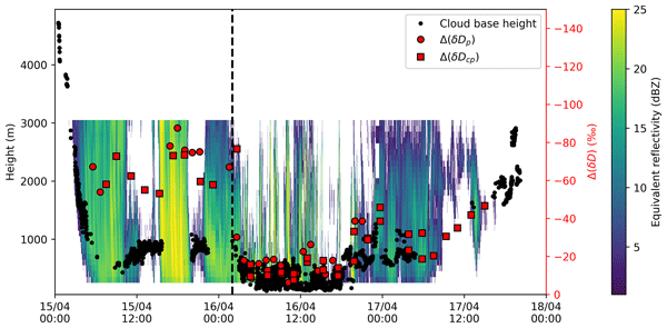
We compare in Fig. 8 the Δ(δD) metric from our new dataset to remote sensing observations, including the cloud base height (CBH) from the ceilometer and the vertical structure of precipitation from the MRR reflectivity (Wiener et al., 2024). We focus below on case study 2, which is associated with the longest precipitation record (approximately 56 h).

Figure 8 Combined view of in-situ isotope observations and remote sensing. Red circles (resp. squares) correspond to the Δ(δD) calculated from online Δ(δD_p) (resp. collected Δ(δD_cp)) precipitation; the black dots correspond to the ceilometer cloud base height and the MRR equivalent reflectivity is plotted in background (color scale). Note that the Δ(δD) axis is plotted on a reversed scale. The vertical dashed line separates the first and second parts of the event, situated on 16 April at 03:00 UTC.

On 15 April 2023, periods of high reflectivity coincide with missing CBH data, indicating ceilometer signal attenuation due to intense precipitation. A sharp descent of the cloud base is observed between 00:00 to 05:00 UTC from ∼4 km to below 1 km, stabilizing between 15 April at 12:00 UTC and early 16 April. The cloud base then further descends to near-surface levels between 04:00 and 17:00 UTC on 16 April. After 16 April at 17:00 UTC, the cloud base rises to ∼850 m with the end of precipitation detected by the radar on 17 April at ∼07:00 UTC. However, snow samples are still collected until 17 April at 16:00 UTC, where the cloud base reaches 2 km. Notably, two periods can be highlighted in Fig. 8: a first part occurring on 15 April before the cloud descent to ground level with low values of Δ(δD) (note that the Δ(δD) y axis is inverted, with lower values at the top), and a second part from 16 April at 03:00 UTC (indicated by the vertical dashed line in Fig. 8) onward, where the Δ(δD) metric shows a higher value and a consistent correlation with cloud base height.

In the first part of the event, from 15 April to 16 April at 03:00 UTC, Δ(δD) shows much lower values, around $\sim -\mathrm{65}$ ‰ with a large variability. During this period, the MRR mostly shows high reflectivity values (10–20 dBZ) extending from the surface up to 3 km, with cloud tops exceeding the radar's observational range. Two local maxima in Δ(δD_cp) are observed on 15 April at approximately 14:00 and 20:00 UTC, each showing an increase of $\sim +\mathrm{20}$ ‰. These maxima coincide with periods when no precipitation is detected from the radar reflectivity, although a delay in the hourly range is observed between the reflectivity gaps and the corresponding Δ(δD_cp) maxima. This delay may reflect the fall time of snow particles and supports the idea that the isotopic signal carries an information related to snow formation conditions.

In the second part of the event, following the descent of the cloud base after 03:00 UTC on 16 April, maximum reflectivity remains below 3 km and is confined to a narrower vertical layer. This more compact vertical cloud extent and lower CBH is associated with a higher value of Δ(δD) (mean value of −23 ‰), compared to the first part of the event. We also note that on 17 April after 07:00 UTC only Δ(δD_cp) is observed (associated exclusively with wind sock samples, see Fig. 4), while no snowflakes entered the inlet and no precipitation signal was detected by the MRR.

On this case study, we observe links between the vertical structure of precipitation and Δ(δD). In the first part of the event, the radar reflectivity suggests that precipitation measured on the ground likely grew on an extended vertical column, from the ground to 3 km and above. During this period, we observe low Δ(δD) values. In the second part, a more compact structure with low clouds is observed, with a correlation between Δ(δD) and the cloud base height. If we assume an idealised situation where snow forms above the observation site under thermodynamic equilibrium, with vapor deposition as the dominant growth process and no isotopic modification during descent, then δD_p,eq can provide a first-order estimate of the isotopic composition of the surrounding vapor during snow formation. In this case the Δ(δD) metric could reflect the temperature or altitude difference between the surface and the mean level of snow formation, provided that the vertical isotopic gradient remains approximately constant.

The vertical structure of clouds and precipitation could explain part of the Δ(δD) intra-event variability, but it is associated with some limitations. First, the fractionation coefficient used to retrieve δD_p,eq and thus the ΔδD metric is based on surface temperature, although the precipitation is formed in altitude at significantly lower temperatures. In addition, in case of snow formation in high level clouds, a time delay is expected between the measurement of the isotopic composition of precipitation at ground level and the remote sensing observations, which is not accounted for here. The Δ(δD) approach also assumes equilibrium fractionation from vapor deposition and does not account for kinetic effects, such as supersaturation, rimed ice growth or snow sublimation. Finally, blowing and drifting snow can dominate the snowflake signal such as in 17 April. These processes can alter the isotopic signal of precipitation and also contribute to variability in Δ(δD).

Additional observations are needed to better constrains these processes. Remote sensing observations are limited by the range (3 km) and the limit of detection (1.14 dBZ, see Wiener et al., 2024) of the micro rain radar, limiting its ability to detect upper cloud layers or resolve fine microphysical structures. This restricts the comparison of the Δ(δD) metric against detailed cloud and precipitation profiles, in particular during the first part of the event. The use of cloud radars with higher sensitivity and range, and advanced capabilities (e.g. multifrequency, scanning, or polarimetric measurements) could provide more detailed insights into cloud processes, including the regions of vapor deposition and riming processes (Planat et al., 2021). Finally, snow imaging instruments providing snowflake size and shape could help disentangle the respective contributions of falling, drifting, and blowing snow near the surface.

5 Conclusion and perspective

We have developed and validated a novel method for online measurement of precipitation isotopic composition using a single laser spectrometer, capable of analyzing both water vapor and solid precipitation. The method was tested across three precipitation events with a wide range of humidity conditions (∼500–5000 ppm), representative of year-round variability on the East-Antarctica coast (Dumont d'Urville station). Comparisons with manually collected snow samples show a mean deviation of −5.4 ‰ in δD and a dispersion of 8.2 ‰, which we attribute mainly to calibration uncertainties and differences in the sampling frequency between online measurement and manual collection. Given that the observed intra-event variability of precipitation δD is on the order of 100 ‰, these uncertainties do not limit the signal interpretation. Compared to manual collection, the automated approach offers clear advantages: it requires no human intervention and is sensitive enough to detect very small precipitation volumes, making it well-suited for deployment in the low-precipitation environments of the Antarctic plateau.

Several technical improvements are foreseen, including the development of an orientable inlet and adjustable diaphragm to increase the likelihood of capturing snowflakes. Future efforts will also focus on enabling measurements of second-order isotopic parameters such as d-excess, which was not achievable with the current AP2E spectrometer setup. At this stage, the method is complementary to manual sampling rather than a full replacement, especially in places with large precipitation amounts, where manual collection provides lower uncertainty and access to second-order parameters.

We then illustrated two applications of this sampling method using our new dataset, representative of coastal regions of East-Antarctica. First, it can be used to better evaluate and constrain isotope-enabled atmospheric models such as LMDZiso for the isotopic composition of falling precipitation before its integration in the snowpack. This opens up new possibilities for evaluating the implementation of cloud processes and their impact on the isotopic composition of precipitation, for improving the representation of snowflake-atmosphere interactions (particularly during sublimation), and for constraining the contributions of falling, drifting and blowing snow, which arise from different transport and transformation pathways. Second, we explored the relationship between surface water vapor and precipitation isotopic composition, and in particular the Δ(δD) metric, as a way to gain insight into snow formation conditions. Its comparison with ceilometer and micro rain radar observations revealed a promising correlation with cloud-base height, indicating that Δ(δD) could help identify key cloud processes such as the altitude of condensation. At this stage, the synergy between Δ(δD) and remote sensing remains limited both by the simplified assumptions underlying the metric and by the restricted vertical range and sensitivity of the micro rain radar. Ongoing deployments will help overcome some of these limitations. For example, the use of polarimetric radars (Planat et al., 2021) or multi-frequency remote sensing (Aubry et al., 2024; Billault-Roux et al., 2023) will allow for more detailed diagnosis of cloud microphysical structure and associated processes.

Finally, over the Antarctic plateau, where post-depositional sublimation strongly alters the surface signal, this technique provides a unique opportunity to directly quantify the isotopic composition of precipitation, even during low-intensity events typically missed by manual sampling. This will improve constraints on the primary isotopic signal and the reliability of ice core climate reconstructions.