Improving the confidence in retrievals of vertical distributions of cloud condensation nuclei number concentration from ARM supported by aircraft in situ observations

Accurate quantification of the vertical distribution of cloud condensation nuclei (CCN) number concentrations is critical for improving our understanding of aerosol–cloud interactions. Ground-based Raman lidars operated by the Atmospheric Radiation Measurement (ARM) program, together with surface CCN measurements, are used to retrieve vertically resolved CCN number concentrations (Retrieved Number concentration of CCN, RNCCN). These retrievals rely on several assumptions, including that aerosol composition is vertically homogeneous. To assess this assumption, we developed and tested a framework to infer the dominant aerosol classes/types at different altitudes. This was done by applying a k-Nearest-Neighbors (kNN) algorithm to lidar ratio and linear depolarization ratio measurements from Raman lidar. We evaluated the framework using aircraft aerosol and CCN measurements from the ARM Holistic Interactions of Shallow Clouds, Aerosols, and Land Ecosystems (HI-SCALE) field campaign. The results show that RNCCN performance degrades as vertical aerosol complexity increases, i.e., RNCCN agrees with the aircraft CCN in vertically homogeneous conditions, but closure decreases in layered aerosol structures. To generalize beyond individual examples, we introduce a metric (heterogeneity index) that quantifies the vertical complexity by assessing the variation in inferred aerosol classes/types. Case-level statistics show a tendency for RNCCN and aircraft differences to increase as this metric increases. By detecting retrievals that are likely compromised by aerosol vertical heterogeneity, the proposed framework improves the interpretability and effective use of RNCCN for long-term evaluation of models and aerosol–cloud interactions.

1 Introduction

Aerosol particles in the atmosphere that serve as cloud condensation nuclei (CCN) are critical to the formation of clouds and influence cloud optical properties and cloud life cycle, thereby affecting the Earth's energy balance and hydrological cycle (Lohmann and Feichter, 2005; Rosenfeld et al., 2014; Dong et al., 2015; Bellouin et al., 2020). These CCN-driven changes in cloud properties are central to aerosol–cloud interactions (ACI) and contribute to aerosol indirect radiative forcing, whose magnitude remains one of the largest uncertainties in Earth system model simulations (Gryspeerdt et al., 2023).

Accurately quantifying ACI critically depends on understanding the vertical distribution of CCN. Ground-based CCN measurements alone are insufficient, as they cannot capture these variations with altitude. CCN in the sub-cloud layer approaching cloud base directly influence the initial number of cloud droplets and subsequent microphysical processes. Consequently, the ability of Earth system models to reliably simulate cloud droplet activation and assess aerosol indirect effects is contingent on the accurate representation of these vertical CCN profiles (e.g., Ghan et al., 2012; Watson-Parris et al., 2019).

Considering the scarcity of in situ aircraft measurements of CCN vertical profiles, lidar observations provide a crucial source of information. Various methods have been developed to retrieve CCN concentrations from spaceborne (satellite), airborne, and ground-based lidar observations. Satellite lidar products, such as aerosol backscatter, extinction, and aerosol type information, are widely used to estimate CCN profiles (e.g., Choudhury and Tesche, 2022a, b; Kapustin et al., 2006; Kulkarni et al., 2025). These estimates complement traditional satellite-derived aerosol products and enable global-scale estimates of CCN (e.g., Shinozuka et al., 2015; Levy et al., 2013).

Airborne lidar provides vertically resolved aerosol profiles along flight tracks. For example, airborne high-spectral-resolution lidars (HSRL) directly measure extinction and depolarization, enabling aerosol-type classification and CCN retrieval without assumptions required by elastic-backscatter systems (Burton et al., 2012). Lenhardt et al. (2023) used airborne HSRL extinction collocated with in situ CCN to derive empirical CCN relationships for biomass-burning aerosol over the southeast Atlantic.

Ground-based lidar approaches also offer higher vertical resolution and have been widely used in CCN retrievals. For example, polarization lidar is combined with AERONET data to classify aerosol types and derive empirical relationships between extinction coefficients and dry particle size thresholds, enabling the estimation of CCN number concentrations (Mamouri and Ansmann, 2016). In addition, a multi-wavelength lidar inversion technique has been applied to retrieve aerosol size distributions from optical properties, thereby estimating CCN concentrations (Lv et al., 2018).

In contrast to the above type-dependent or inversion-based approaches, “extinction-based” methods estimate CCN profiles by combining vertically resolved lidar extinction with a near-surface CCN constraint, avoiding the need for multi-wavelength microphysical inversions or aerosol-type-specific parameterizations. This provides a computationally simple and operationally robust pathway for continuous CCN profiling when only standard lidar products are available (Shinozuka et al., 2015; Lenhardt et al., 2023; Ghan et al., 2006). Specifically, Ghan et al. (2006) and McFarlane et al. (2012) derived CCN number concentration profiles by scaling surface CCN measurements using vertically resolved aerosol extinction from Raman lidar, enabling application at sites with routine surface CCN observations and standard lidar observations. Building on this concept, Chen et al. (2025) retrieved aerosol vertical profiles by combining micropulse lidar with ground-based aerosol measurements during the Tracking Aerosol Convection Interactions ExpeRiment (TRACER) campaign in Texas. The U.S. Department of Energy's Atmospheric Radiation Measurement (ARM) user facility developed the Retrieved Number Concentration of CCN (RNCCN) product based on Ghan et al. (2006)'s methodology (Kulkarni et al., 2023b), providing continuous estimation of vertical distributions of CCN number concentration (Brendecke et al., 2022; Kulkarni et al., 2025).

One of the underlying assumptions within the RNCCN calculation is that aerosol properties (e.g., type, shape) are vertically uniform (i.e., invariant with height). However, this assumption could be invalid, especially when heterogeneous aerosol layers aloft are observed (e.g., Clarke et al., 1997; Fast et al., 2022; Russell et al., 2014; Seinfeld et al., 2016). Consequently, evaluating RNCCN requires explicitly identifying conditions where aerosol properties vary or remain invariant with height. We hypothesize that deviations from the vertical uniformity assumption of aerosol properties may lead to systematic discrepancies between RNCCN and in situ CCN (e.g., with large errors expected under more vertically heterogeneous aerosol conditions). To test this hypothesis, we need (1) a method to diagnose vertical aerosol heterogeneity from available remote-sensing observables and (2) in situ CCN data that can be used to quantify how such heterogeneity impacts RNCCN accuracy.

Aerosol properties' vertical heterogeneity can be inferred through variations in aerosol optical properties. Lidar measurements offer a powerful tool for detecting and characterizing these variations (e.g., Ferrare et al., 2023, 2025; Groß et al., 2025; Müller et al., 2007; Nicolae et al., 2026; Omar et al., 2009; Papagiannopoulos et al., 2018; Redemann and Gao, 2024; Sugimoto et al., 2002). Two key lidar-derived parameters, linear depolarization ratio (LDR) and lidar ratio (LR), provide insight into aerosol shape, composition, and size. The LDR distinguishes spherical particles (e.g., pollution, smoke) from non-spherical ones (e.g., dust, ash), while the LR reflects differences in aerosol composition and size distribution (Burton et al., 2012; Groß et al., 2015; Müller et al., 2007).

Recent advances in machine learning (ML) offer the potential for more automated and robust aerosol classification from lidar observations, particularly when multi-wavelength or fluorescence capabilities are available (del Águila et al., 2025; Nicolae et al., 2018; Peleg et al., 2026; Veselovskii et al., 2022). Such ML frameworks typically depend on specialized instrumentation and often require synthetic training datasets or site-specific tuning, which may limit their broader applicability. These limitations pose difficulties for applying existing ML methods to a specific lidar (e.g., the DOE ARM Raman lidar), which operates at a single wavelength (355 nm) and lacks fluorescence detection. To address this gap, we need to develop a new classification approach tailored to a single-wavelength Raman lidar.

High-quality in situ data from both surface and aircraft collected by the DOE ARM program provide an opportunity for us to investigate whether vertical heterogeneity in aerosol properties (e.g., type, shape, or composition) impacts the reliability of RNCCN retrievals. The Holistic Interactions of Shallow Clouds, Aerosols, and Land Ecosystems (HI-SCALE) field campaign, conducted in spring and summer 2016 near the Southern Great Plains (SGP) Central Facility, deployed research aircraft to collect vertically resolved CCN and aerosol measurements across a range of land surface types (Fast et al., 2019). Using this dataset, it has been found that the extinction-based RNCCN method outperforms satellite- and model-based estimates in reproducing airborne CCN observations (Kulkarni et al., 2025). Building upon this understanding and complementing this finding, our study focuses on identifying and quantifying conditions, particularly vertically heterogeneous aerosol structures diagnosed from lidar observables, under which RNCCN retrieval confidence may be reduced.

This study introduces a framework to relate vertical heterogeneity in aerosol optical properties to RNCCN retrieval error and confidence. We test the hypothesis that vertically heterogeneous (layered) aerosol conditions, diagnosed by height-dependent variations in lidar ratio and linear depolarization ratio, produce larger CCN retrieval errors than vertically homogeneous (well-mixed) aerosol layers. To validate this, we compare CCN profiles retrieved using the standard RNCCN assumption of vertically uniform aerosol properties against in situ aircraft measurements and quantify how retrieval errors vary as the diagnosed heterogeneity increases.

2 Data

This study uses multi-platform ARM observations to develop and evaluate an aerosol type classification framework. Aerosol types are classified based on the DeLiAn (Depolarization ratio, Lidar ratio, and Ångström exponent, details in Sect. 2.1) database using ARM Raman lidar (RL) observations (Sect. 2.2). The RNCCN (Sect. 2.3) is compared with G-1 aircraft CCN measurements (Sect. 2.4) to test our hypothesis.

2.1 Aerosol Type Database

The DeLiAn database (Floutsi et al., 2023) is utilized in this study because it provides the comprehensive aerosol optical properties needed to develop an aerosol classification framework. To our knowledge, DeLiAn is one of the most extensive and up-to-date datasets for aerosol typing for ground-based lidar, making it invaluable for aerosol classification tasks. Its data and classifications have been widely used to inform aerosol schemes for the EarthCARE mission (Wandinger et al., 2023) and satellite-based algorithms, such as CALIPSO's aerosol subtype classification (Kim et al., 2018; Tackett et al., 2023).

The DeLiAn database compiles lidar parameters (LDR and LR) and aerosol optical properties (Ångström exponent) from ground-based Raman and polarization lidars operated at 355, 532, and 1064 nm. Values are typically derived in cloud-free conditions and represent aerosol layers identified within the lowest few kilometers of the troposphere, where the ground-based lidars provide the most reliable aerosol retrievals. The database includes 13 aerosol classes: 10 basic aerosol types (clean marine, dried marine, pollution, Central European background, tropospheric smoke, stratospheric smoke, volcanic ash, Saharan dust, Central Asian dust, and Middle Eastern dust) and three mixtures (dust and smoke, dust and pollution, and dust and marine). These measurements are conducted by the Leibniz Institute for Tropospheric Research (TROPOS) using advanced lidar systems (Engelmann et al., 2016) deployed at fixed EARLINET sites (Pappalardo et al., 2014) and mobile platforms, including ship-based campaigns (Bohlmann et al., 2018; Engelmann et al., 2021; Kanitz et al., 2013). The data span diverse geographic regions, including Europe, the Middle East, Central Asia, North Africa, and marine environments.

This study uses the DeLiAn dataset, specifically the aerosol types inferred from the lidar parameters (LR and LDR) and their reported uncertainties (i.e., the reported standard deviations reflecting layer-averaging, instrument noise, and calibration uncertainty) at 355 nm. We use the 355 nm subset because it matches the wavelength of the ARM Raman lidar used to generate the RNCCN product.

2.2 ARM Raman Lidar

ARM RL observations from the SGP site are used. The RL provides vertical measurements of aerosol backscatter, extinction, LR, and LDR at 355 nm, with vertical and temporal resolutions of 30 m and 2 min, respectively. The dataset is available through the Raman Lidar Profiles-Feature detection and Extinction (RLPROF-FEX) Value-Added Product (VAP) (Thorsen et al., 2015; Thorsen and Fu, 2015; Chand et al., 2019). A direct evaluation of the RLPROF-FEX aerosol extinction profiles against in situ measurements is unavailable. However, comparisons of RLPROF-FEX aerosol optical depth with sun-photometer measurements at the SGP site yielded relative Root Mean Square Error (RMSE) values of approximately 32 %–43 % and systematic biases of about −3 % (Thorsen and Fu, 2015).

2.3 ARM CCN Vertical Profile

To estimate vertical CCN concentrations, this study uses the RNCCN VAP developed by DOE ARM (Kulkarni et al., 2023b, 2025), based on the method developed by Ghan and Collins (2004) and Ghan et al. (2006). This VAP provides vertical profiles of CCN concentration at 10 min temporal resolution and 60 m vertical resolution, by scaling surface CCN measurements using dry-corrected aerosol extinction profiles (also provided within RNCCN VAP), which are derived from Raman lidar observations. The RNCCN concentration at a given height z, time t, and supersaturation SS is calculated as:

$$\begin{array}{}\text{(1)}& \begin{array}{rl}\text{RNCCN}(z,t,\text{SS})& =\text{CCN}(\mathrm{0},t,\text{SS})\\ & \times \left[{\mathit{\alpha }}_{\text{dry}}(z,t)/{\mathit{\alpha }}_{\text{dry}}(\mathrm{0},t)\right]\end{array}\end{array}$$

where $\text{CCN}(\mathrm{0},t,\text{SS})$ is the surface CCN concentration, and α_dry(z,t) and α_dry(0,t) are the dry-corrected aerosol extinction values at height z and the surface, respectively.

Surface-based CCN measurements at various supersaturation values are obtained from the DOE ARM dual-column CCN-200 instrument (Uin and Enekwizu, 2024). The instrument reports CCN number concentrations as a function of supersaturation, at 1 Hz resolution. During standard operation, the instrument cycles through six supersaturation levels per hour, ranging from 0 %–1.0 %, with each level maintained for several minutes.

The dry extinction profile is computed by adjusting the ambient extinction profile from RLPROF-FEX using a relative humidity (RH)-dependent aerosol humidification factor, f(RH), parameterized with a gamma coefficient (γ) that reflects the sensitivity of extinction to RH (Dawson et al., 2020; Zieger et al., 2010). The gamma value is empirically derived for each day from collocated extinction and RH profiles. This correction ensures that the extinction profile reflects dry aerosol conditions, which are more directly related to the CCN measurements.

Various quality control tests are applied to generate the RNCCN dataset. RL profiles with missing RH and aerosol mask features are excluded (Kulkarni et al., 2025). RH profiles that exceed 85 % are omitted to avoid large, highly uncertain hygroscopic-growth corrections. Temperature profiles (Newsom et al., 2018; Newsom and Sivaraman, 2018) that report supercooled temperatures are also excluded because mixed-phase/cloud contamination can bias the Raman retrievals and the associated extinction-to-CCN scaling. These filters reduce data availability during some cold-season periods, but do not eliminate wintertime RNCCN retrievals overall. Further, extinction profiles are also filtered using feature masks (Chand et al., 2019; Thorsen et al., 2015; Thorsen and Fu, 2015) to remove cloud and precipitation layers. RNCCN can still be retrieved in aerosol-only regions below cloud base; however, profiles (or portions of profiles) flagged as precipitation are excluded because the mask is no longer classified as aerosol, and reliable extinction retrievals are not available. Because of high uncertainty from the instrument's near-field overlap, the extinction values at the lowest measurement level, the first range gate (i.e., the first discrete altitude interval above the ground where the lidar returns are processed), can be larger than 0.4 km⁻¹or below 0.02 km⁻¹(Kulkarni et al., 2025). When the first range gate extinction falls within the acceptable range (0.02–0.4 km⁻¹), it is used because it is closest to the surface CCN measurement and best represents the near-surface aerosol used to anchor the scaling. When it falls outside this range, the extinction value from the second range gate is used for RNCCN estimation.

2.4 ARM G1 Aircraft data during HI-SCALE campaign

We used in situ CCN measurements collected during the 2016 HI-SCALE campaign near the SGP site. The SGP site is situated in a rural, mid-latitude continental setting surrounded by heterogeneous land use, including cultivated crops, pastures, grasslands, and forested regions. The campaign comprised two intensive observational periods (IOPs): a spring IOP (24 April–21 May 2016) and a summer IOP (28 August–24 September 2016). Although the SGP site is often regarded as a relatively clean continental location, the aerosol population sampled during HI-SCALE was complex and originated from a mixture of anthropogenic, biogenic, and biomass burning sources (Fast et al., 2019). Meteorological conditions during the campaign were variable. Larger aerosol concentrations were generally associated with warm, mostly sunny conditions and southerly winds that favored photochemistry and the transport of anthropogenic emissions from Oklahoma City and urban areas in Texas, whereas the lowest concentrations occurred under northerly or westerly flow that advected cleaner air over the site (Fast et al., 2019). Although HI-SCALE targeted shallow convective clouds, the campaign also sampled clear-sky days, more complex multi-layer cloud populations, and periods preceding or following deep convection (Fast et al., 2019).

The aircraft sampled vertical aerosol and meteorological profiles, with CCN concentrations measured at 1 Hz using a dual-column CCN counter operating at fixed supersaturations of 0.24 % and 0.46 % (Uin and Mei, 2019). We focused on the 0.24 % channel to compare with extinction-based RNCCN estimates because the activation dry diameters corresponding to this SS contributed significantly to the extinction (Kulkarni et al., 2025). The uncertainty in the in situ CCN concentration is generally within approximately 20 %, based on the CCN closure analysis in Kulkarni et al. (2023a). Only data obtained under cloud-free conditions were used. The high temporal and vertical resolution of the G-1 data, averaged to 10 min intervals, provided a benchmark for evaluating RNCCN retrieval uncertainty.

3 Methodology

We used a k-Nearest Neighbors (kNN) classifier to map Raman-lidar observations into aerosol-type classes defined in the DeLiAn database. The DeLiAn is used here as a labeled training dataset rather than as a lookup table. Each DeLiAn entry provides a pair of optical observables (LR and LDR) together with an expert-assigned aerosol-type label, which we treat as “truth”. The kNN classifier learns the relationship between these optical observables and aerosol types from the DeLiAn data and is then applied to predict an aerosol type for each ARM Raman-lidar observation using only its measured LR and LDR as input. In other words, DeLiAn supplies the training labels, while the ARM lidar supplies the new (unlabeled) observations to be classified.

3.1 k-Nearest Neighbors: Model Configuration and Training

The kNN classifier was implemented in Python using scikit-learn (KNeighborsClassifier; Pedregosa et al., 2011). kNN is a versatile algorithm and requires only a few user-specified parameters, primarily the number of neighbors (k) and a distance metric, making it straightforward to implement in this study. As a non-parametric ML method, it does not impose a predefined functional form on the decision boundary (i.e., the surface in feature space that separates different aerosol/CCN regimes). Instead, it learns this boundary directly from the data, which allows it to capture nonlinear relationships and still perform robustly with relatively small training datasets, making it a practical choice for this study.

The kNN method is implemented using LDR and LR as input features. For each new observation, kNN searches the DeLiAn database for the k most similar samples (i.e., closest in the LDR–LR feature space) and assigns the aerosol type based on the majority class among those nearest neighbors. The development of our kNN classifier involved three key stages with careful design: (A) curating the source dataset, (B) augmenting the data to create a balanced training set, and finally (C) training and optimizing the model. These stages are discussed as follows.

• A.

  To adapt the kNN model for the continental SGP site, we refined the standard DeLiAn training dataset by curating its “marine” aerosol class. The default DeLiAn marine definition (LDR<5 %, $\text{LR}\approx \mathrm{30}-\mathrm{40}\text{sr}$) overlaps strongly with SGP pollution and would tend to misclassify pollution as marine despite typically weak marine influence at SGP (Liu et al., 2021). Moreover, field observations indicate that typical marine aerosols exhibit very low depolarization (<3 %) and lower LR ($\sim \mathrm{20}-\mathrm{25}\text{sr}$) (Groß et al., 2025; Illingworth et al., 2015). We find that the anomalously high LR values in the DeLiAn marine class are mainly associated with rare shipborne “dried marine” cases from cruises, where sea-salt particles are modified by dry free-tropospheric air (Haarig et al., 2017). Thus, we excluded these non-representative cruise samples to improve climatological consistency and reduce misclassification. After filtering, the remaining DeLiAn “marine” class mainly occupies the low-LDR/low-LR corner. At the continental SGP site, the resulting “marine” label should be interpreted as a clean/background optical regime (low LDR, low LR) rather than true sea-salt influence; supporting analysis is provided in Appendix A.

• B.

  The DeLiAn database (Floutsi et al., 2023) for aerosol types is shown in Fig. 1a. Here, the aerosol-type classification is performed using paired measurements of LDR (%) and LR (steradian, sr) at 355 nm. Several aerosol types in the DeLiAn database contain only a small number of observations. To prevent these sparsely sampled classes from being overwhelmed by well-sampled types in the kNN voting step, we apply an uncertainty-aware augmentation procedure. For each observation, synthetic samples are generated by perturbing LDR and LR within their reported measurement uncertainties, using a truncated range to avoid unrealistic values. We then balance the training set by expanding each aerosol type to 61 samples, the size of the largest well-sampled class in the original DeLiAn dataset (Smoke; 61 valid observations). All other classes are augmented to this size (Fig. 1b), ensuring comparable representation across aerosol types without oversampling beyond the existing majority class.

• C.

  During training, LDR and LR are standardized using statistics from the augmented dataset (i.e., the DeLiAn observations plus the uncertainty-perturbed synthetic samples). We use a kNN classifier with Euclidean distance and distance-weighted voting (i.e., closer neighbors receive higher weights in the class assignment), chosen for its non-parametric nature and its ability to represent the locally clustered structure of aerosol types in LDR–LR space. The number of neighbors (k) is selected via 5-fold stratified cross-validation for hyperparameter tuning. Within each fold, augmentation and standardization are applied only to the training subset, scaling parameters are computed from the augmented training data, to prevent information leakage into the held-out fold. The value of k with the highest mean macro-averaged F1 score (a standard metric that balances precision and recall across all classes) is used in all subsequent analyses. Final model training is performed on the full augmented dataset and LDR–LR observations that are standardized and classified using this trained model.

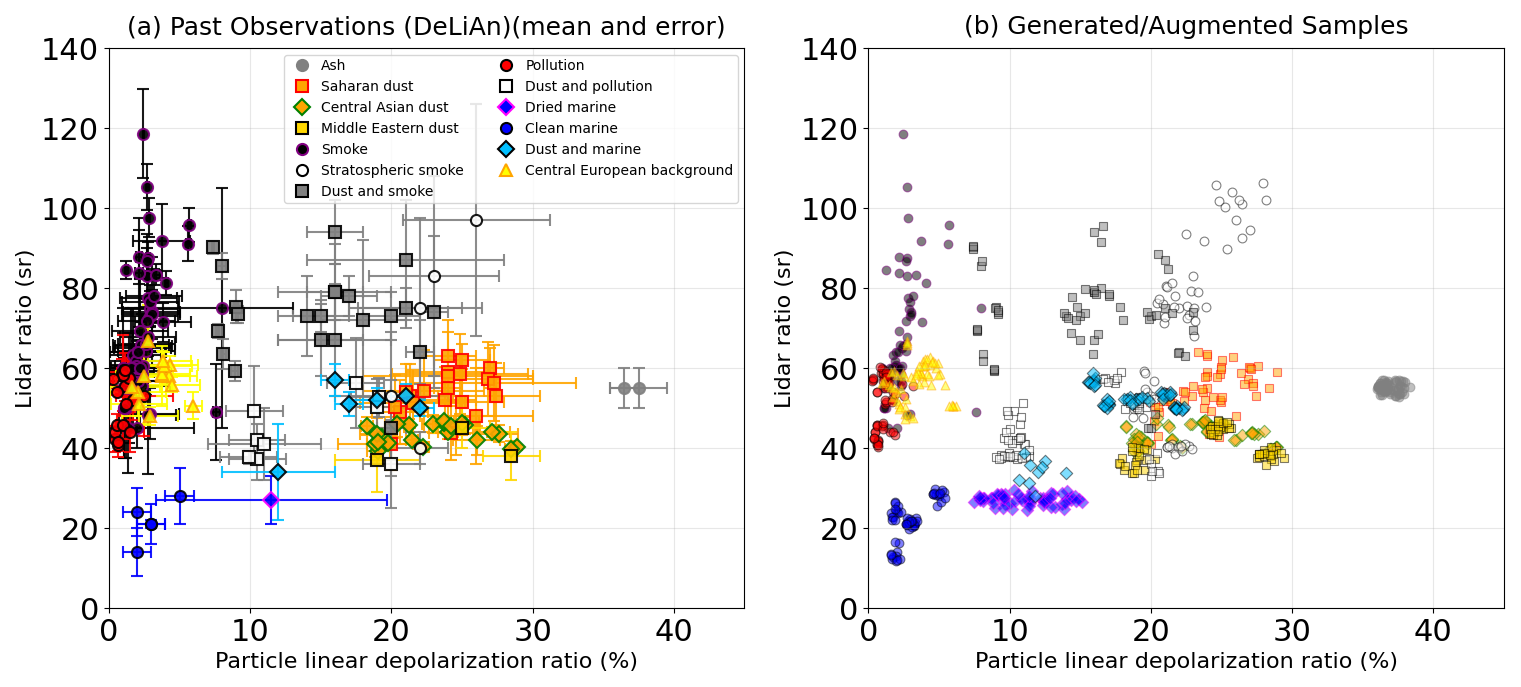
Figure 1 (a) DeLiAn aerosol linear depolarization ratio vs. lidar ratio observations at 355 nm showing the original measured points with their reported uncertainties (error bars) (reproduced using data in Floutsi et al., 2023). (b) Training dataset after uncertainty-aware augmentation: each original observation is supplemented by synthetic samples generated by perturbing LDR and LR within the reported uncertainties, so that each aerosol type contains 61 samples. Colors denote the 13 aerosol types.

3.2 ML Model Performance

The kNN classifier's performance was assessed through a separate 5-fold stratified cross-validation using the selected k. For each fold, the training data portion was independently augmented using the uncertainty-aware procedure described in Sect. 3.1, ensuring that the model is always evaluated on held-out data untouched by the augmentation. Predictions for each test fold were then collected and aggregated to generate the final performance metrics.

The resulting row-normalized confusion matrix is shown in Fig. 2. Each row corresponds to the true aerosol class and each column to the predicted class; values indicate the fraction of samples in a true class assigned to each predicted class. Darker diagonal elements indicate more accurate classifications, while off-diagonal elements highlight systematic confusion between classes.

We merged aerosol classes into broader categories to improve the interpretability of the confusion matrix while preserving dominant optical similarities. Specifically, Marine combines Clean marine and Dried marine; Dust combines Saharan dust, Central Asian dust, and Middle Eastern dust; Pollution/Central European Background (CEB) combines Pollution and Central European background, because the CEB type largely represents aged continental anthropogenic aerosol, it is also grouped with pollution in the final aerosol classification; and Smoke combines Smoke and Stratospheric smoke. All other categories (Ash, Dust and smoke, Dust and pollution, Dust and marine) remain unchanged.

The confusion matrix is shown in Fig. 2. Optically distinct classes are retrieved with high fidelity: “Ash” is classified perfectly (1.00), and key fine-mode anthropogenic regimes are well resolved, including Pollution/CEB (0.83) and Smoke (0.66). In contrast, ambiguity increases among dust and mixed classes with overlapping LDR–LR signatures. For example, “Dust and marine” is frequently confused with “Dust” (0.33) and “Dust and pollution” (0.67). “Dust and pollution” is split between its correct label (0.67), “Dust and marine” (0.22), with the remaining fraction assigned to “Dust” (0.11). This is consistent with the limited separability of mixtures using only two optical features. Higher-fidelity discrimination would require additional independent observables (e.g., multiwavelength backscatter/extinction or spectral depolarization), which is beyond the scope of this LR–LDR-only framework. Importantly, most misclassifications occur among closely related dust/mixed categories that occupy similar regions of LR–LDR space, rather than between fundamentally different regimes. Because our application is to diagnose vertical heterogeneity and layer structure, not to provide definitive aerosol composition, the classifier skill should be sufficient for identifying transitions between distinct optical regimes.

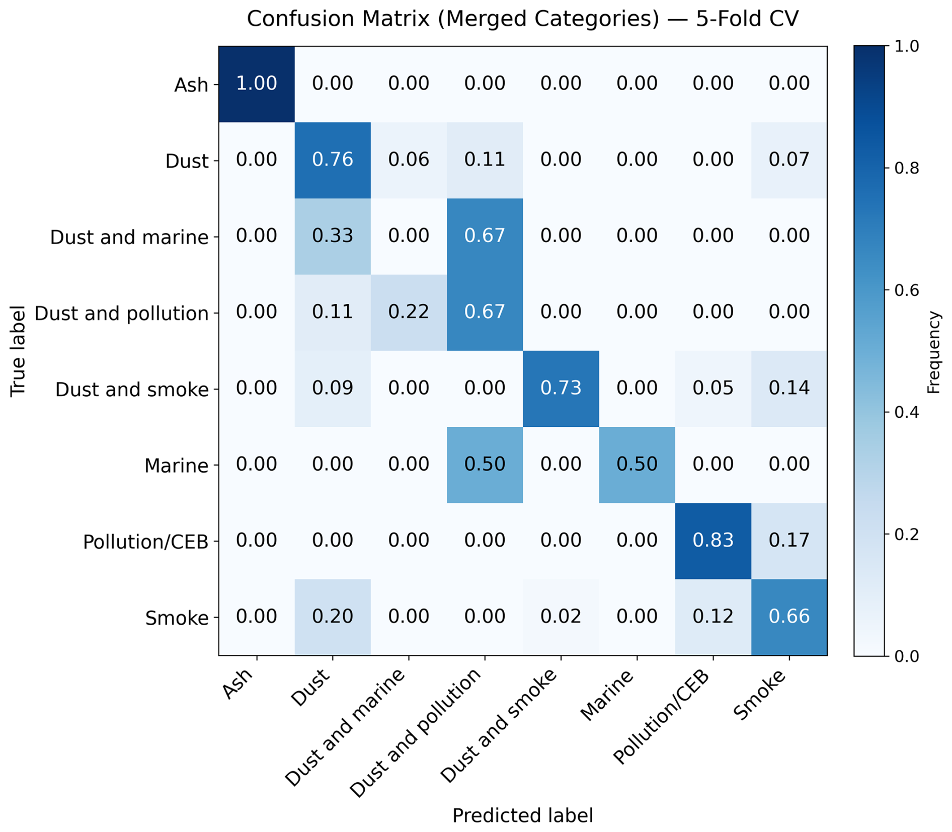
Figure 2 Row-normalized confusion matrix for the kNN aerosol-type classifier using merged DeLiAn categories, based on 5-fold stratified cross-validation. Rows denote the true class, and columns denote the predicted class; diagonal elements give the per-class recall (classification accuracy), and off-diagonal elements show the fraction misclassified into other classes. The corresponding confusion matrix for the original (unmerged) DeLiAn classes is shown in Appendix Fig. B1.

In addition, this kNN-based framework assumes that the major aerosol types encountered at SGP are reasonably represented in the DeLiAn training set and that Raman-lidar LR and LDR provide meaningful signatures for separating those types. As with any lidar-based typing approach, uncertainties arise from the instruments' calibration drift and low-SNR conditions, which can reduce classification confidence. Because kNN assigns types based on similarity in LR–LDR space, mixed aerosol and observations near class boundaries may occasionally blur distinctions among categories. Accordingly, the inferred types should be interpreted as an optical-regime diagnostic rather than a definitive statement of aerosol composition. This caveat is important to keep in mind when interpreting RNCCN behavior under complex or heterogeneous aerosol conditions.

4 Results and Discussion

4.1 Case-Based Evaluation of RNCCN

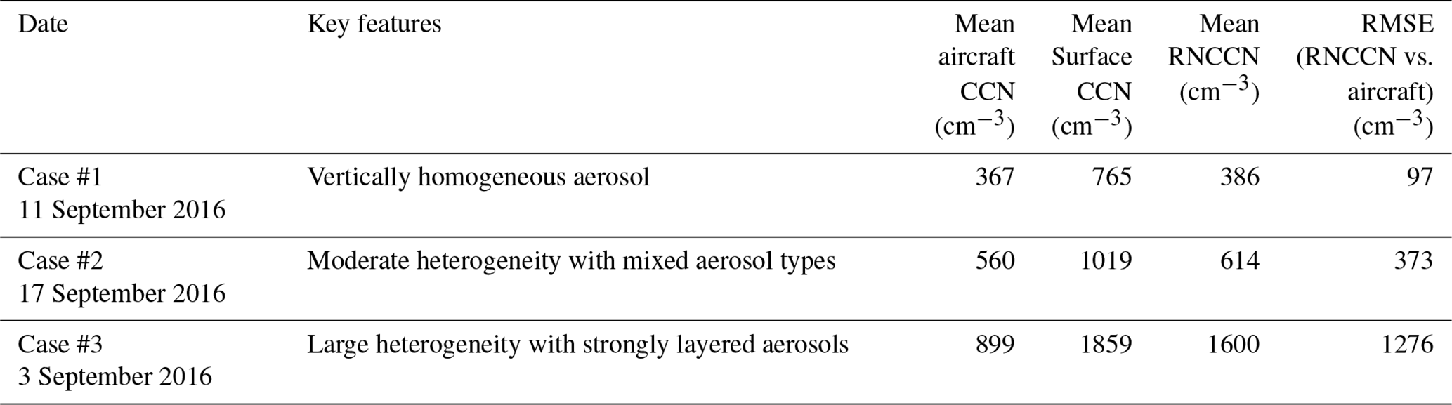
In this section, we first focus on case studies from HI-SCALE periods when in situ CCN measurements and RNCCN retrievals are available. These cases enable a very detailed examination of how aerosol type classification helps interpret differences between aircraft in situ CCN measurements and retrieved RNCCN values. To ensure comparability, we selected cases where (1) the G1 remained within 100 km (radially) of the Raman lidar site and (2) the aircraft operated below the planetary boundary layer height (PBLH; Zhang et al., 2022). For detailed case analysis, we selected three flight days: 3, 11, and 17 September 2016. These cases (summarized in Table 1) span a range of aerosol conditions from vertically homogeneous (case #1) to highly heterogeneous (case #3), with case #2 in between.

Table 1 Summary of RNCCN performance for the three HI-SCALE case days.

4.1.1 Case 1: Vertically Relative Homogeneous Pollution

Figure 3 presents a case from 11 September 2016 characterized by relatively stable aerosol properties and limited vertical variability in LDR and LR from 15:10–18:10 UTC. The time–height evolution of LDR (Fig. 3a) shows consistently low values (<2 %), while LR (Fig. 3b) remains mostly between 30 and 60 sr. In the DeLiAn database (Fig. 1a), this region of LDR–LR space is dominated by pollution aerosols; our ML model also identified this period as pollution (Fig. 3c).

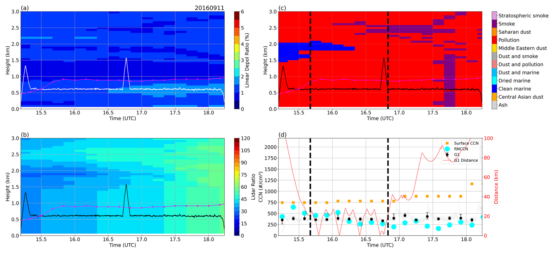
Figure 3 Time–height cross sections on 11 September 2016 (Case #1): (a) LDR (%) from Raman lidar, with the white line showing G-1 aircraft altitude and magenta line the planetary boundary layer height from Doppler lidar; (b) same as (a), but for lidar ratio (sr); (c) aerosol type classification from the kNN model; (d) time series of in situ CCN concentration aboard the G-1 at 0.24 % supersaturation (black circles: median, with 25th–75th interquartile range), overlaid with collocated RNCCN retrievals (cyan circles) and surface CCN (orange squares). The red line (right axis) shows aircraft distance from the SGP Raman lidar; vertical dashed lines indicate the period of interest (e.g., when the aircraft was within ∼30 km of the site).

The comparison between retrieved RNCCN and in situ CCN concentrations is shown in Fig. 3d. During 15:40–16:50 UTC (between the dashed lines), when the G-1 aircraft remained within ∼30 km of the Raman lidar, RNCCN agrees closely with the aircraft CCN measurements. This distance threshold (30 km) is chosen because the RNCCN product is averaged over 10 min intervals, during which the aircraft typically travels about 60 km at $\sim \mathrm{100}\mathrm{m}{\mathrm{s}}^{-\mathrm{1}}$; a 30 km radius therefore approximates the spatial footprint of the lidar retrieval. Within this 30 km radial vicinity, the mean aircraft CCN concentration is 367 cm⁻³, and the collocated RNCCN retrievals have a mean value of 386 cm⁻³, an RMSE of 97 cm⁻³, and a small positive bias of $\sim \mathrm{19}{\mathrm{cm}}^{-\mathrm{3}}$ (Table 1). This indicates a slight systematic overestimation of CCN by RNCCN under well-collocated, vertically homogeneous conditions.

In contrast, surface CCN measurements (orange squares) are substantially higher than both RNCCN and aircraft CCN, often by roughly a factor of two. This behavior demonstrates that near-surface CCN concentrations are not always representative of CCN aloft, even during relatively uniform aerosol conditions.

Even as the aircraft distance from the Raman lidar increases later in the period (red curve in Fig. 3d), RNCCN remains broadly consistent with the in situ measurements, indicating horizontal homogeneity in aerosol type and loading in this case. Overall, Case #1 represents a near-ideal condition/scenario for applying the RNCCN method: a stable aerosol with minimal vertical structure and high classification confidence, resulting in comparatively low CCN retrieval uncertainty compared to aircraft measurements.

4.1.2 Case 2: Moderately Heterogeneous, Mixed Aerosol Types

In contrast to the previous case, Fig. 4 illustrates a more complex boundary layer structure from 17 September 2016, characterized by pronounced vertical and temporal variability. The time–height cross sections (Fig. 4a–c) reveal a multi-layered aerosol structure, with distinct layers of high-LR “Pollution” and “Smoke” overlying a layer of low-LR “Clean marine” aerosol (interpreted as a clean/background regime at SGP; see Sect. 3.1 and Appendix A) around 1 km.

Figure 4 Same as Fig. 3, but for the case of 17 September 2016 (case #2).

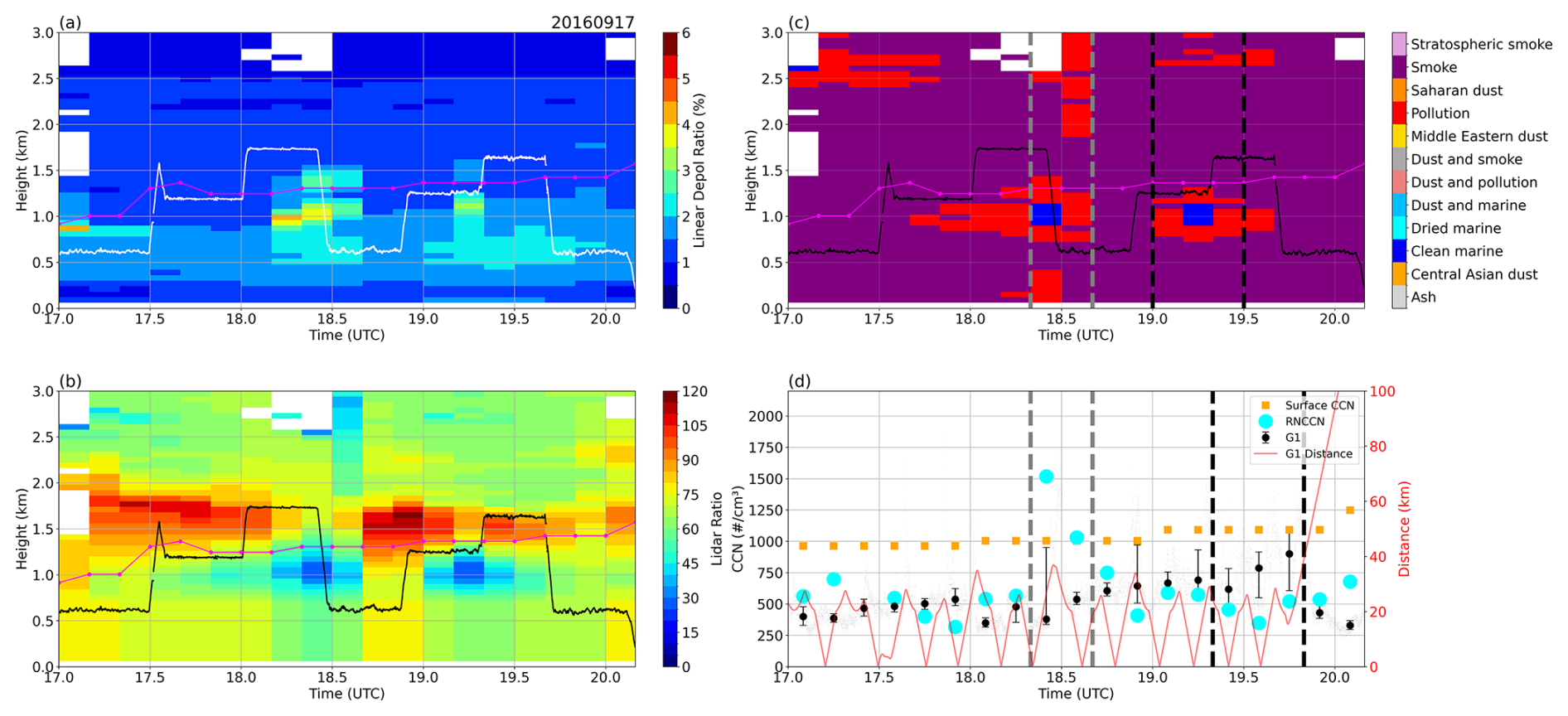
This increased complexity is reflected in the RNCCN performance. For samples when the aircraft was within 30 km of the Raman lidar, the mean aircraft CCN concentration is 560 cm⁻³, while the corresponding RNCCN retrievals exhibit an RMSE of 373 cm⁻³ and a positive bias of $\sim \mathrm{54}{\mathrm{cm}}^{-\mathrm{3}}$ relative to the aircraft (Table 1). These errors are larger than in Case #1.

Large discrepancies between RNCCN and in situ CCN tend to occur when aerosol conditions are vertically and horizontally heterogeneous. For example, large RNCCN–aircraft CCN differences occur in the final two points after ∼ 19:30 UTC, following a period of strong vertical variability in aerosol type (19:00–19:30 UTC; Fig. 4c). The ∼20 min offset can be explained by the lack of exact collocation: the aircraft sampled within a 30 km radius rather than directly above the lidar, so the aircraft and lidar likely sampled different air parcels that advected past the site at slightly different times under heterogeneous conditions.

The most pronounced deviation occurs near 18:30 UTC. Two factors likely contribute: (a) a vertical mismatch in aerosol type between the surface, the column sampled by the lidar, and the aircraft level, such that the vertical homogeneity assumption underlying the RNCCN retrieval is not satisfied, and (b) a rapid change in aircraft altitude during 18:20–18:30 UTC, which increases the variability of the time-averaged CCN estimate, as indicated by the large error bar on the G-1 measurements in this interval (Fig. 4d). Overall, Case #2 demonstrates that RNCCN can still capture the broad magnitude and variability of CCN under moderately heterogeneous conditions, but retrieval errors increase when multiple aerosol types and sharp vertical transitions in aerosol types are present.

4.1.3 Case 3: Strongly Layered Aerosols

Figure 5 shows a case from 3 September 2016 (Case #3) that exhibits greater structural complexity than the previous cases. In Fig. 5a and b, the LDR and LR fields reveal a strongly layered aerosol structure, and the aerosol-type classifications (Fig. 5c) alternate between pollution, smoke, and occasional marine-like signatures. Grid cells without an assigned aerosol type at around 1 km in Fig. 5c correspond directly to a “clean-air (no-detected-feature)” layer (Fig. C1c), which indicates that no aerosol (or cloud/precipitation) feature is confidently detected and/or that aerosol extinction cannot be retrieved with sufficient quality in that layer (Thorsen et al., 2015).

Figure 5 Same as Fig. 3, but for the case of 3 September 2016 (case #3).

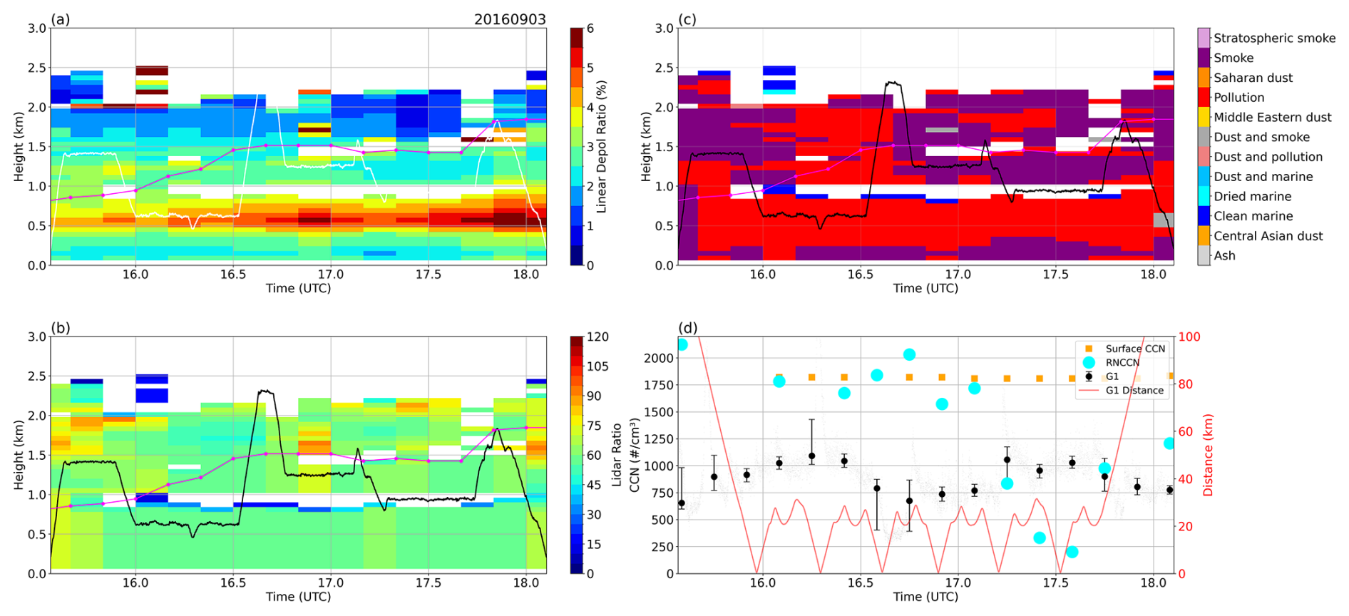
The RNCCN algorithm relies on the ratio of dry extinction at height z to the surface value. This scaling requires valid, quality-controlled extinction retrievals at the reference level and at height z and a vertically continuous extinction profile between them. As a result, RNCCN is not reported within these clean-air (no-feature) layers. Where RNCCN is reported above the gap, its interpretation may be uncertain because the extinction scaling is effectively applied across a layer with missing or low-quality extinction, so the connection between the surface aerosol and the elevated layer may not be confidently established.

The comparison with in situ CCN measurements (Fig. 5d) reflects this case's complexity. Overall, RNCCN performance is much worse than in the first two cases. For samples collected within 30 km of the Raman lidar, the mean aircraft CCN concentration is 899 cm⁻³, whereas RNCCN exhibits an RMSE of 1276 cm⁻³ and a substantial positive bias of 701 cm⁻³ (Table 1). These large discrepancies indicate that the retrieval substantially overestimates CCN under these heterogeneous, multi-layered aerosol type conditions.

The degraded performance coincides with (1) vertically intermittent clean-air (no-feature) regions that break the column into poorly constrained segments and (2) pronounced aerosol-type variability with height. Unlike Case #1, where the aerosol column was relatively uniform and well classified, this example highlights conditions in which the RNCCN assumption of a vertically homogeneous, well-characterized sub-cloud aerosol layer is clearly not held, leading to larger retrieval uncertainties.

4.2 Statistical Evaluation of RNCCN

While the case studies in Sect. 4.1 provide a detailed, qualitative view of RNCCN performance under specific conditions, they do not indicate how representative those behaviors are across the full HI-SCALE dataset/cases. A statistical analysis is necessary to generalize the case-study findings to all available flights and relate RNCCN deviation from aircraft measurements to a more objective measure of aerosol complexity.

To examine how aerosol variability influences RNCCN performance, all G-1–RNCCN comparisons were aggregated into 10 min windows over the overlapping aircraft and RNCCN observation period for each flight day. For each window, the G-1 CCN concentration was calculated by averaging all available valid 1 Hz G-1 observations. Window-level statistics were retained only when (i) the resulting G-1 and RNCCN values were finite, and (ii) the mean aircraft–Raman lidar distance separation was less than 30 km. Only flight days with more than three valid windows were included in the case-level analysis.

To quantify the complexity of the aerosol column for each case, we use the kNN aerosol-type classifications derived from Raman lidar measurements (LDR and LR). For every valid 10 min window that meets the collocation criteria described above, and for all RNCCN vertical levels between the surface and the maximum aircraft altitude, we count occurrences of each aerosol type and the clean-air (no-detected-feature) category, which represents layers where aerosol extinction is not retrievable and can interrupt the extinction scaling used by RNCCN. Counts are summed over all valid windows for a given case and converted to fractional occurrences p_i. A simple heterogeneity index is then defined using the Gini impurity (Breiman et al., 1984):

$$\begin{array}{}\text{(2)}& H=\mathrm{1}-\sum _i{p}_i^{\mathrm{2}},\end{array}$$

such that H closes to 0 corresponds to a nearly uniform aerosol column dominated by a single type, while larger values reflect increased mixing among multiple aerosol types and/or substantial no-feature (extinction-retrieval gap) layers below the aircraft.

For each case, we compute the mean G-1 CCN and RNCCN CCN across all valid windows and use $\left|\text{RNCCN-G1}\right|$ as a case-level measure of retrieval error. Figure 6 summarizes the relationship between vertical heterogeneity below aircraft flight altitude and RNCCN performance. Each point represents a flight segment, labeled by its case ID. The 20160911 case (Case #1 in Sect. 4.1.1) (H≈0) exhibits a vertically uniform aerosol environment with minimal type transitions and no missing layers and correspondingly shows the smallest RNCCN–G-1 difference, whereas larger discrepancies occur for cases with elevated heterogeneity (e.g., H>0.5).

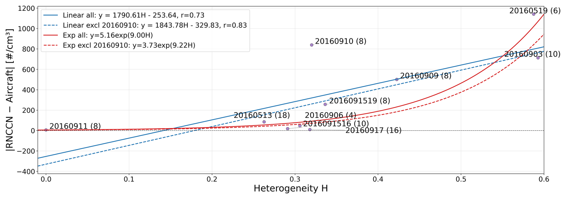
Figure 6 Case-level relationship between aerosol heterogeneity H and RNCCN Aircraft difference |RNCCN–Aircraft|. Cases are labeled by date (YYYYMMDD); when more than one qualifying flight segment occurred on the same day, the central UTC hour is appended (YYYYMMDDHH; e.g., 2016091516 and 2016091519). Solid lines represent linear and exponential fits using all cases, while dashed lines exclude the 20160910-outlier case.

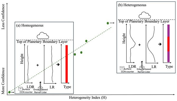
Overall, Fig. 6 shows a modest positive association between RNCCN–G1 discrepancies and heterogeneity index, although substantial scatter remains at intermediate H. A linear fit indicates moderate correlations (0.73 or 0.83 when excluding 10 September 2016), consistent with an overall increase in discrepancy with H. This conclusion/trend holds when the error is expressed as either an absolute difference or a relative difference normalized by the mean G1 CCN. This result supports the interpretation that the extinction-scaling approach used in RNCCN is more likely to produce large errors in vertically complex/heterogeneous conditions (larger H values), not just in the specific examples shown in Figs. 3–5. Figure 7 provides a conceptual overview of the diagnostic framework, contrasting vertically homogeneous and heterogeneous aerosol conditions and illustrating their influence on RNCCN retrieval performance.

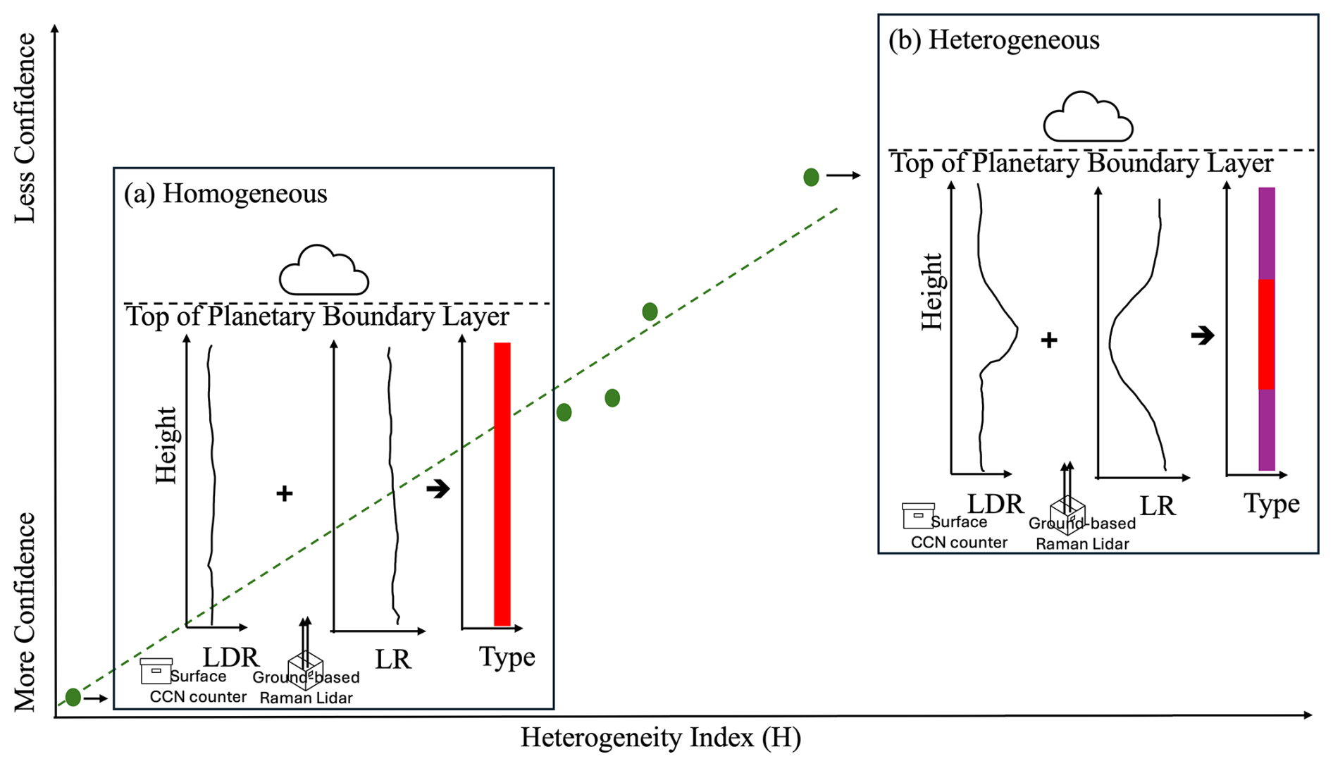
Figure 7 Conceptual overview of the analysis framework. The two panels contrast vertically homogeneous and heterogeneous aerosol conditions, and their influence on RNCCN retrieval performance. Green dots represent conceptual case-level relationships between aerosol vertical heterogeneity and the RNCCN–aircraft difference, while the dashed green line illustrates the overall trend of increasing RNCCN–aircraft difference (i.e., decreasing retrieval confidence) with increasing aerosol vertical heterogeneity.

The surface-anchored RNCCN method is best suited to the boundary layer: scaling a surface CCN measurement by the surface-normalized extinction ratio (Eq. 1) assumes surface aerosol is representative of aerosol aloft, more valid in PBL but generally not in the free troposphere, where decoupled or transported layers can differ substantially from the surface. We therefore restrict the RNCCN evaluation to the PBL. However, the diagnostic tool developed here (kNN typing and the heterogeneity index H) is not subject to this limitation, as they rely only on lidar LR and LDR and can be applied throughout the column to flag elevated, decoupled layers.

At the same time, we emphasize that H summarizes heterogeneity in LR/LDR-derived aerosol typing and should therefore be interpreted as an indicator of vertical-complexity rather than a complete predictor of RNCCN error. RNCCN discrepancies can also be driven by strong vertical extinction gradients and/or retrieval and representativeness uncertainties that are not fully captured by H; the 10 September 2016 outlier is discussed in Appendix D.

5 Summary and Conclusions

The objective of this study is to assess how vertical variability in aerosol optical properties (used as a proxy for aerosol type/compositional variability) affects the performance of CCN profiles provided by the ARM RNCCN. This assessment was carried out using in situ aircraft CCN measurements from the HI-SCALE field study conducted near the ARM SGP site.

The RNCCN retrieval method relies on scaling surface CCN measurements with vertically resolved aerosol extinction profiles from Raman lidar and assumes a vertically uniform aerosol composition. However, this assumption may not always be valid, and therefore, this study specifically investigated whether the vertical variability in lidar-inferred aerosol classes (based on lidar ratio and linear depolarization ratio) can serve as an indicator of reduced RNCCN retrieval confidence. We hypothesized that violations of this vertical uniformity assumption, i.e., strong vertical heterogeneity in these lidar-inferred classes, would degrade RNCCN performance. To test this hypothesis, we developed a kNN-based classification framework using data from the DeLiAn database. This framework was used to generate the vertical distributions of aerosol classes. Under different boundary layer vertical aerosol variations, we then compared RNCCN with in situ CCN concentrations from the G-1 aircraft.

The results show that RNCCN performance degrades as vertical aerosol complexity increases. For vertically homogeneous, pollution-dominated columns, RNCCN closely matches aircraft CCN, indicating that extinction scaling works well when aerosol composition is nearly uniform. As embedded layers of differing aerosol classes/types and moderate vertical structure appear, RNCCN errors grow. In strongly layered scenes with alternating aerosol classes/types, intermittent no-feature regions, or gaps that disconnect elevated aerosol from the surface layer, the difference between RNCCN and aircraft-measured CCN is large.

To generalize beyond individual examples, we introduced a heterogeneity index based on the vertical distribution of kNN-derived aerosol classes/types. Statistics show a tendency for RNCCN retrieval error to increase with this heterogeneity metric (H), quantitatively confirming that aerosol complexity is one of the key controls on RNCCN reliability, even though RNCCN discrepancies can also be driven by strong vertical extinction gradients and/or retrieval and representativeness uncertainties that are not fully captured by H.

This method can be used to enhance RNCCN, either within the existing product or as a companion dataset, by providing kNN-derived aerosol-class/type (optical regime) profiles and a heterogeneity index (H) together with simple quality flags that classify columns as relatively homogeneous or heterogeneous. These additions offer a practical indicator of RNCCN confidence and enable objective filtering or stratification of RNCCN profiles in subsequent analyses. In practice, H can be computed for each RNCCN profile using a temporal window (e.g., 30–60 min) and over a specified lower-tropospheric layer (e.g., 0–3 km). A categorical quality flag can also be assigned from H to distinguish higher-confidence homogeneous cases from lower-confidence heterogeneous cases.

The proposed ML-based assessment framework improves our ability to interpret RNCCN accuracy and to identify conditions under which extinction-scaling approaches are relatively trustworthy. This supports more robust use of long-term CCN vertical distributions (e.g., for Earth system model evaluation). The framework is not limited to the current RNCCN implementation and can be extended to other CCN-profile retrievals from Raman or high-spectral-resolution lidars, provided that both LR and LDR are available. Future work could refine the classification scheme by incorporating additional, independent lidar observables (e.g., multiwavelength backscatter or depolarization), thereby improving aerosol classification based on optical properties and RNCCN assessment in more complex aerosol environments.

In addition to vertical variations in aerosol type, humidity-dependent aerosol growth is another source of CCN retrieval uncertainty: as RH approaches saturation, water uptake increases aerosol extinction and complicates the extinction-to-CCN relationship. The RNCCN product accounts for this effect by converting ambient to dry extinction via an f(RH) correction and excludes observations with RH>85 %, where this correction becomes increasingly uncertain. Improved high-RH humidification parameterizations could broaden the applicability of RNCCN.

Appendix A

This section evaluates the physical meaning of the kNN-derived “marine” aerosol class at SGP and clarifies how this label should be interpreted when assessing RNCCN performance at SGP. Because the SGP site is far from any oceanic influence, a truly sea-salt–dominated aerosol could be unlikely. To investigate whether this classification is physically plausible, we compared independent aircraft measurements from the Aerosol Mass Spectrometer (AMS), Fluorescent Aerosol-Size Time-of-Flight Mobility Spectrometer (FIMS), and SPLAT (Single Particle Laser Ablation Time-of-Flight Mass Spectrometer).

For each flight day, AMS provided non-refractory submicron mass (sulfate, nitrate, ammonium, chloride, organics), while FIMS measured the full aerosol size distribution, which includes AMS-detectable species plus coarse-mode dust and any potential sea-salt (Fast et al., 2022). To estimate aerosol mass from FIMS, we used composition-dependent effective densities derived from SPLAT, which reports per-case fractional contributions of major aerosol classes. Combining the FIMS size distribution with SPLAT-derived effective density allowed us to infer a bulk mass concentration that should exceed AMS if marine or dust aerosols were abundant.

For 10 September 2016, the FIMS-inferred mass was not significantly larger than AMS, and both instruments showed relatively low aerosol loading compared to other flight days (Fig. A1). This may indicate that this case was not dominated by sea salt or dust. Instead, it appears to represent a clean, low aerosol airmass. Under such conditions of extremely weak aerosol signal, the LDR–LR features that drive the kNN classification become less distinctive, and the algorithm can misclassify “clean” conditions as “marine” because both exhibit weak depolarization and moderate lidar ratios. Thus, we suspect that the “marine” label does not imply the presence of sea salt but is better interpreted as a clean background regime with very low continental aerosol influence. This interpretation is consistent with ARM's use of the term “clean marine” in remote regions (e.g., Kennaook–Cape Grim), where it denotes an airmass with minimal anthropogenic or continental contributions, not necessarily one dominated by oceanic sea-salt particles. Overall, our analysis suggests that the marine classification at SGP may reflect the absence of pollution, rather than true marine aerosol.

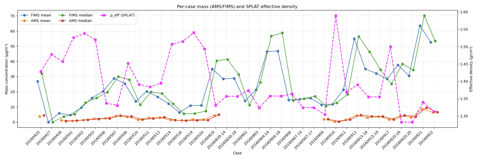
Figure A1 Per-case aerosol mass derived from the Fast Integrated Mobility Spectrometer (FIMS) and the Aerosol Mass Spectrometer (AMS), together with Single Particle Laser Ablation Time-of-Flight Mass Spectrometer (SPLAT)–derived effective particle density (ρ_eff). FIMS aerosol mass (mean and median) is estimated from measured aerosol size distributions using the case-specific effective density (ρ_eff), while AMS mass represents non-refractory submicron aerosol species, including sulfate (${\mathrm{SO}}_{\mathrm{4}}^{\mathrm{2}-}$), nitrate (${\mathrm{NO}}_{\mathrm{3}}^{-}$), ammonium (${\mathrm{NH}}_{\mathrm{4}}^{+}$), chloride (Cl⁻), and organic aerosol (Org).

Appendix B

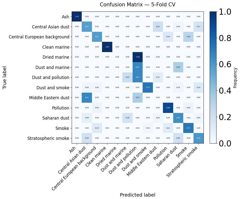
Figure B1 Row-normalized confusion matrix from 5-fold stratified cross-validation. Each row represents the true aerosol class, and each column shows the predicted class. Values on the diagonal represent the accuracy for each class, while off-diagonal values indicate misclassifications.

Classification performance is type-dependent. The model demonstrates high fidelity in distinguishing optically unique aerosol types (“Ash”, “Smoke”, “Pollution”, and “Clean Marine”). For example, “Ash” and “Clean marine” are identified with near-perfect accuracy. The classifier also effectively resolves key anthropogenic types like Pollution (89 % accuracy) and Smoke (72 % accuracy). Conversely, and as expected, classification ambiguity increases for aerosol classes with overlapping optical properties. This is most evident among different dust types and mixtures. For instance, the model struggles to differentiate regional dusts: 67 % of “Middle Eastern dust” is misclassified as “Central Asian dust”. Similarly, mixed aerosol classes are challenging. While “Dust and pollution” is correctly identified 67 % of the time, the remaining 22 % (11 %) is misclassified as “Dust and marine” (“Middle Eastern dust”), indicating confusion between a mixture and one of its potential pure components. These patterns do not indicate a model failure, and they are consistent with the expected difficulty of distinguishing internally mixed or regionally similar dust types using only LDR and LR.

Appendix C

The feature masks shown in Fig. C1 are derived from the Raman Lidar Profiles, Feature Detection and Extinction (RLPROF-FEX) Value-Added Product (VAP) (Chand et al., 2019). The RLPROF-FEX algorithm identifies and classifies atmospheric targets, including aerosol layers, liquid clouds, ice clouds, and precipitation, using automated feature detection methods described in Thorsen et al. (2015) and Thorsen and Fu (2015).

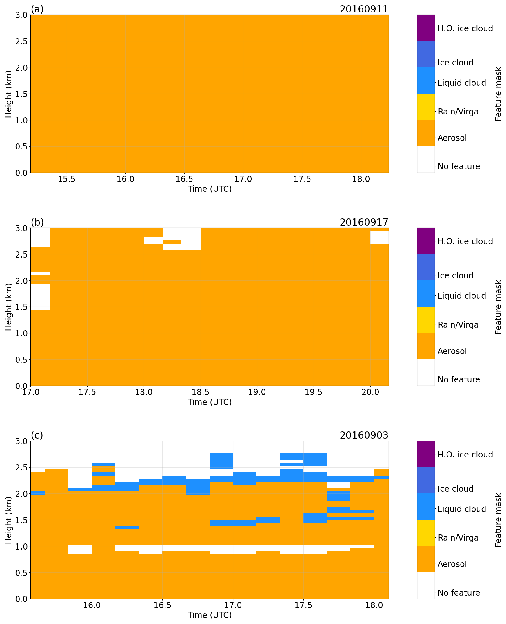
Figure C1 Feature mask from Raman Lidar on (a) 11 September 2016 (case #1), (b) 17 September 2016 (case #2), and (c) 3 September 2016 (case #3).

Appendix D

In Fig. D1d (case 10 September 2016), RNCCN substantially overestimates the aircraft CCN. This bias is not accompanied by a substantial change in LR or LDR with height, and the kNN classifier assigns the same aerosol type at the surface and flight level, probably suggesting that the error is not driven by a major aerosol-type transition in LR–LDR space. Instead, the Raman-lidar dry-corrected extinction increases sharply with height during this period (Fig. D2), yielding an unusually large dry-extinction ratio relative to the near-surface reference level. Because RNCCN scales surface CCN by this ratio, the enhanced extinction gradient directly amplifies the retrieved CCN aloft and explains the overestimate mechanistically.

Figure D1 Same as Fig. 3, but for the case of 10 September 2016.

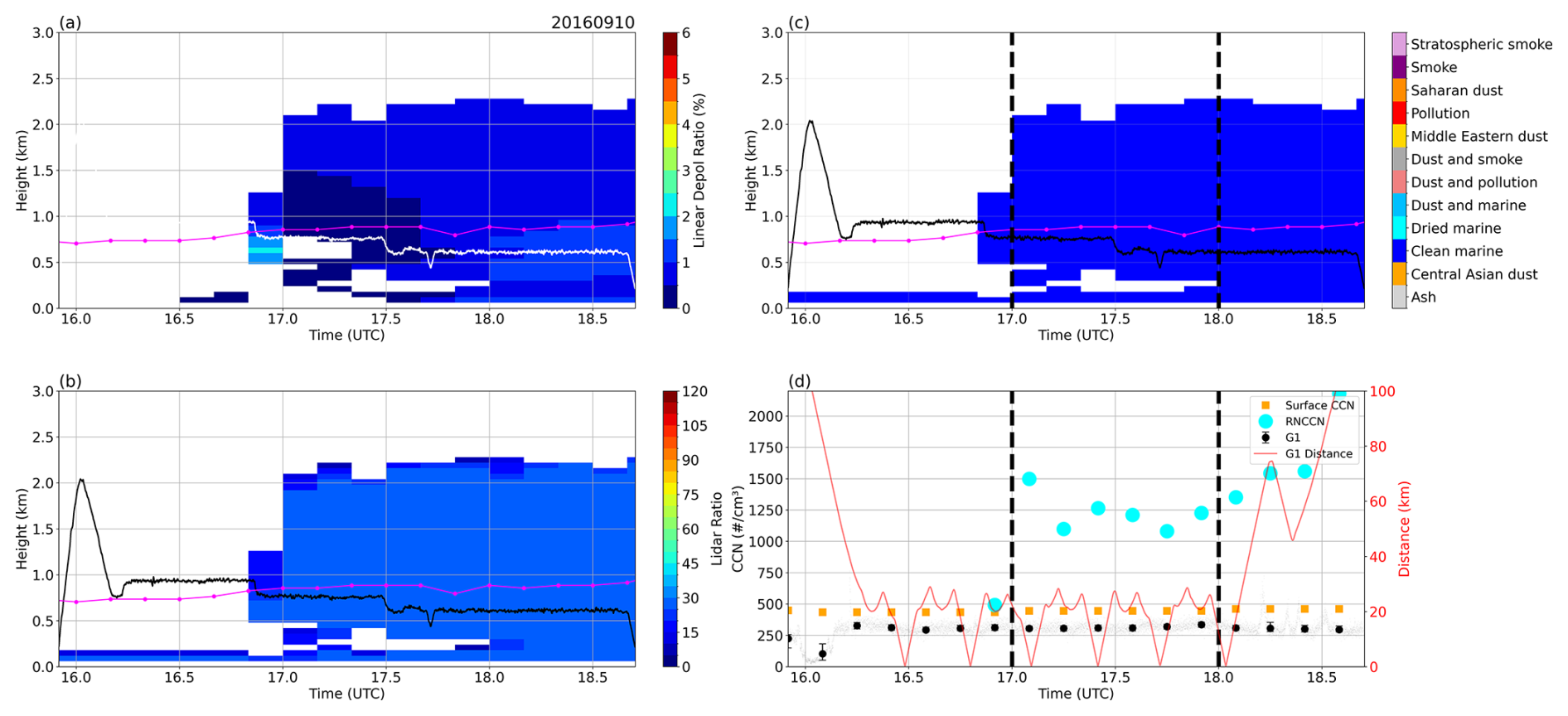
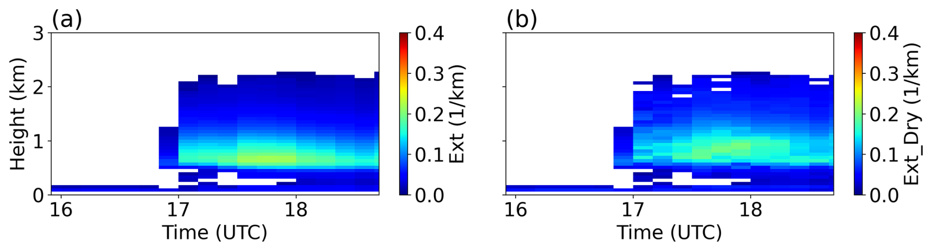
Figure D2 Time–height cross sections of Raman-lidar aerosol extinction for the case on 10 September 2016. (a) Lidar extinction coefficient (Ext, km⁻¹). (b) Dry-corrected aerosol extinction coefficient (Ext_Dry, km⁻¹) directly used in the RNCCN.

The origin of this extreme extinction gradient cannot be uniquely determined here. One physical possibility is: an elevated aerosol layer with substantially higher aerosol loading and/or different microphysical characteristics than near the surface, even though LR and LDR remain within the same kNN aerosol-type class (i.e., similar LR–LDR does not imply vertically uniform loading or a constant extinction-to-CCN relationship). Alternatively, the gradient may be influenced by retrieval and representativeness effects, for example, low-SNR/QC limitations (including the intervening no-feature interval), and/or imperfect spatial–temporal matching between the aircraft and the surface–lidar column despite the less than 30 km distance.