An update to the expression of atmospheric refractivity for GNSS signals

This study revisits previous formulations of atmospheric refractivity at L-band frequencies, focusing on signals from Global Navigation Satellite Systems (GNSS). A refined model expression is proposed as a function of air density, temperature, and composition, evaluated using a comprehensive set of existing laboratory and atmospheric measurements. The key measurements that most affect the final accuracy are identified, establishing traceable error bounds and indicating where further experimental work could confirm or improve the model.

Recent studies on the use of large volumes of GNSS radio occultation (GNSSRO) observations in Numerical Weather Prediction (NWP) show that the precise formulation of refractivity becomes increasingly critical as data volumes grow. Although the revision is modest, its impact lies within the range where NWP sensitivity becomes non-negligible.

Compared to earlier work, this study (1) incorporates updated fundamental measurements, (2) accounts for the small but measurable variability in atmospheric composition, mainly increasing CO₂ and decreasing O₂, emphasizing that refractivity traceability is composition-dependent, and (3) extends the model to include hydrometeors. A simplified formulation based on hydrometeor oblateness is proposed, suitable for NWP applications where only limited hydrometeor information is available. Nonspherical hydrometeors tend to align during fall, introducing weak birefringence that can be detected during GNSS occultations with dual-polarization receivers.

The resulting refractivity expression is presented as a function of air density, temperature, moisture, and composition, and (using a simplified model of atmospheric evolution) also as a function of density, temperature, moisture, and time. It is concluded that the result meets the target accuracy of 0.01 %, with all remaining uncertainty sources below this threshold. With respect to earlier work, composition and hydrometeor additions do not modify the largest part of the bulk refractivity above this threshold.

1 Introduction

Global Navigation Satellite System (GNSS) Radio Occultation (GNSSRO) is a technique for remote sensing of the Earth's atmosphere (Melbourne et al., 1994; Kursinski et al., 1997). It has proven highly useful for operational numerical weather prediction, (e.g. Healy and Thépaut, 2006; Cucurull et al., 2007; Aparicio and Deblonde, 2008; Rennie, 2008; Poli et al., 2009), and climate research, (e.g. Anthes et al., 2000; Steiner et al., 2011), providing high-resolution vertical profiles of temperature and humidity.

A major reason for this success is the excellent absolute calibration of GNSSRO. The data are derived from highly accurate and traceable frequency observations, a procedure that is intrinsically robust against instrumental bias. For thermodynamic measurements of the atmosphere, GNSSRO has established a qualitatively new traceability link to the International System of Units (SI), complementing in-situ instruments such as surface thermometers, radiosondes, and aircraft sensors.

Although no measurement is entirely free from error or bias, radio occultation provides observations of exceptionally high raw precision. How much of this precision can be translated into accuracy in the retrieved atmospheric variables remains an open question. The issue is linked, on one hand, to the interpretation of raw measurements in terms of specific propagation paths (e.g. Ao et al., 2003; Sokolovskiy, 2003; Xie et al., 2010), and on the other, to the connection between the radio-optical and thermodynamic properties of air, expressed through the refractive index as a constitutive relation). This latter connection is the focus of this study.

A previous investigation (Aparicio and Laroche, 2011), hereafter referred to as AL11, concluded that for this constitutive relation, an average accuracy of 0.1 % can be routinely achieved in linking the radio-optical and thermodynamic properties of air (i.e. refractivity, pressure, temperature and moisture). It also concluded that current understanding of the relevant physics should allow an accuracy of 0.01 %. Accurate laboratory measurements of air's constitutive properties already exist, but to exploit these and achieve accuracy better than 0.1 %, proper attention must be given to the precise definitions of thermodynamic quantities, to the equation of state of moist air and its deviations from ideal-gas behaviour, to the various standard formulations of atmospheric humidity (specific and relative humidity, vapour pressure, dew-point depression, etc.), and to the strongly non-ideal behaviour of water vapour. Such considerations are essential not only when formulating constitutive relations and their parameters but also, and most importantly, during their routine use in NWP.

For these reasons, the simplest approach for a user may be to accept that an accuracy better than 0.1 % is unlikely to be achieved. In this case, the thermodynamic details of the air equation of state or the representation of water vapour concentration are not especially demanding. However, achieving an additional order of magnitude in accuracy is realistic and can be valuable for many scientific and operational applications. Such a goal has been expressed, for example, by CGMS (2012), to improve the traceability of radio occultation data for both weather forecasting and climate research. The motivation is twofold: first, to ensure that the use of GNSSRO data is not limited by uncertainties in the constitutive relations, and second, to provide SI-traceable estimates of the accuracy of these relations.

It is therefore assumed hereafter that exceeding the 0.1 % accuracy level is of interest. To ensure traceability, it is not only desirable that the resulting expressions are as accurate as possible, but also that their uncertainties be quantifiable and attributable to specific sources. On the other hand, achieving accuracy better than 0.01 % does not appear realistic at present. Accordingly, the analysis presented here focuses on this intermediate range of accuracy.

Recently, in connection with the Radio Occultation Meteorology Experiment (ROMEX, Anthes et al., 2024), several studies have addressed the expansion of radio-optical GNSS measurements to volumes significantly higher than those available over the past two decades. The number of global GNSSRO profiles has increased from about 10 000 profiles per day, typical in major NWP centers since the launch of the COSMIC-2 mission (Schreiner et al., 2020), to between 20 000 and 40 000 global profiles per day. The impact of GNSSRO data, already substantial, generally increases with the higher volume, but also becomes more sensitive to details of data processing and assimilation.

NWP systems are highly sensitive to biases between expected and observed data. While instrumental biases may sometimes need correction, it is common practice to apply bias correction simply to ensure statistical consistency between forecasts and observations (see Eyre, 1992, 2016). GNSSRO measurements, however, are known to exhibit very low intrinsic bias. Therefore, they should not be bias-corrected solely for statistical alignment; rather, it is preferable to ensure that the traceability link between the radio-optical and thermodynamic properties of air remains as bias-free as possible.

In the present context, “sufficiently free of bias” is taken to mean “accurate enough that NWP systems do not perceive a bias originating from GNSSRO data”, even when used at the highest practical data volumes, currently about 40 000 profiles per day. Both the earlier AL11 formulation and the expression presented here have been tested with these enhanced volume experiments in the global NWP system at Environment and Climate Change Canada (ECCC), as part of the ROMEX studies. In both cases, the results were found to be sufficiently free of bias in the sense defined above, albeit with some differences discussed below. Since the GNSSRO perceived bias against a model is a complex combination of many elements, and the refractivity model is only one of them, a summary of the prime among those in these tests is given in the discussion section. Within ECCC, refractivity, either AL11 or this work, coupled with a suitable equation of state, is not currently viewed as a source of concern towards GNSSRO bias, while it had been in the past (Aparicio et al., 2009; Aparicio and Laroche, 2015).

An ansatz expression is developed here as an extension of AL11, together with an associated error budget. AL11 has already proven valuable in operational forecasting environments, improving the consistency among different SI-traceability links of atmospheric measurements, notably against radiosondes and aircraft data (Aparicio and Laroche, 2015), and leading to enhanced forecast performance. Both AL11 and the updated ansatz expression proposed here are similar to existing ones in the literature but differ in recommending the use of density as an independent variable rather than pressure. This choice allows a refractivity expression independent of the equation of state, since air shows measurable deviations from ideal-gas behaviour, already noticeable in dry air and increasingly relevant when water vapour is present.

The motivation for this expansion in scope beyond AL11 is twofold. First, some properties of air are imperfectly known; second, certain properties are known not to be static. Both must be included in the error budget. Regarding imperfect knowledge, the dielectric response of air's constituents (mainly N₂, O₂, etc.) to an electromagnetic wave is known with finite accuracy. Regarding variability, even if the molecular properties were perfectly known, the composition of air is not fixed in space and time. The most obvious source of variability is the moisture content, already explicit in standard refractivity formulations. However, the composition of dry air is also variable, albeit to a lesser extent. Records of CO₂ and O₂ concentration (Keeling et al., 2001; Keeling, 2015a, b) indicate that dry air is not an immutable mixture. Several modes of variability can be identified in these records: global drift, seasonal, geographical, and vertical. Most are small in amplitude for the purpose of this study, and their effect on refractivity is below the target accuracy defined above. Of all the variability modes in the composition of dry air, this work focuses on the largest one, the long-term global drift associated with the measurable accumulation of CO₂ in the atmosphere and the associated decrease in O₂.

The main microphysical model describing the molecular response of gas-phase air to an electromagnetic wave remains unchanged from Aparicio and Laroche (2011). However, the sources of information have been revised to provide error bounds traceable to specific laboratory measurements. Some microphysical elements have been incorporated, notably allowing air to be treated as a multiphase heterogeneous mixture, described as an effective medium: a gaseous matrix that may contain small inclusions of liquid (drops), or solid water (ice, snow). As long as these heterogeneities are small, the medium is effectively homogeneous at the scale of the test electromagnetic field. With GNSS wavelengths in the range λ_GNSS=0.18–0.26 m, this approximation applies to rain drops, ice particles, and snowflakes in the atmosphere, all small with respect to λ_GNSS.

Compared to AL11, the accuracy of the various input parameters has been reassessed, and the most critical ones identified, to determine which limit the overall accuracy of the final model and to apportion the net uncertainty among contributing sources. An updated refractivity expression is then presented. Although the differences relative to the earlier AL11 expression are small, they may be significant for certain applications. Most of the dry-air difference arises from a slightly revised composition of dry air. The new expression and its accompanying error analysis enable several additional applications.

First, specific laboratory measurements that are critical to the model's accuracy are identified, linking the reliability of the refractivity expression directly to the accuracy of those experimental data. Second, the dependence of refractivity on atmospheric composition is made explicit, which may be relevant to decadal-scale climate studies. Since composition is slightly time-dependent, the thermodynamic relationship between refractivity, pressure, moisture, and temperature effectively becomes time-dependent as well. Third, hydrometeors are included. Expressions for their contribution have been presented previously (e.g. Kursinski et al., 1997; Zou et al., 2012), and the main results obtained here are consistent with those studies. However, the dependence on hydrometeor shape is explicitly explored, as nonspherical particles tend to reorient during fall, leading to anisotropic shape distributions that interact differently with each polarization component of the signal. Whereas specific microphysical studies of refractivity and polarization effects for individual ice-crystal habits are ongoing (Padullés et al., 2023, and references therein), this work provides an estimate of refractivity dependence on general hydrometeor shape properties. Because NWP systems typically have limited information about hydrometeors, this analysis focuses on two key parameters: the density of water in hydrometeor form (as a fraction of air) and the hydrometeor oblateness as perceived by the electromagnetic signal. Including this anisotropy enables estimates of polarimetric effects. Users should evaluate whether these two parameters suffice for their purposes or whether more detailed scattering models for specific ice or snow shapes are required.

The various aspects of the microphysical model, relating molecular properties, atmospheric composition, hydrometeor presence, and refractivity are developed in Sect. 2. This model is then applied under a range of conditions to produce a fit suitable for practical use, in Sect. 3. This fit contain several adjusted parameters whose precise value depend on input measurements. An uncertainty analysis of the fit attributes the main sources of parameter uncertainty and identifies which measurements are most critical, indicating where updated experimental data could improve model performance. This analysis is discussed in Sect. 4, along with the differences relative to the earlier AL11 model and to other existing expressions. Finally, in Sect. 5, user expressions are recommended.

2 Microphysical model of the air

The expression of atmospheric refractivity combines two largely independent aspects: (1) the relationship between the electromagnetic response and the number of molecules in an air parcel, and (2) the relationship between the number of molecules and the parcel's mass or density. The first depends on molecular polarizability and dipole, whereas the second is governed by molecular mass.

A microphysical model linking molecular properties (polarizability, electric and magnetic dipoles, and molecular mass) to macroscopic refractivity was described in AL11. The present study follows a similar approach, updating the selection of experimental data. AL11 described a single-phase gaseous medium, which with minor modifications is retained here as the gas phase of atmospheric air. In the present work, the model is extended to a potentially multiphase mixture, allowing for small liquid or solid inclusions (droplets or snow, not necessarily spherical) may be present. Inclusions (solid or liquid) are assumed to occupy small fractions of the total volume and mass, and to be much smaller than the electromagnetic wavelength. Under these conditions the mixture can be treated as a homogeneous effective medium (Garnett, 1904; Bruggeman, 1935).

The microphysical model is here reviewed briefly. The refractive index of the effective medium will follow Maxwell's equation (Born and Wolf, 1999, Sect. 1.2):

$$\begin{array}{}\text{(1)}& n=\sqrt{{\mathit{ϵ}}_{\mathrm{r}}{\mathit{\mu }}_{\mathrm{r}}}\end{array}$$

where ϵ_r and μ_r are the relative electric permittivity and magnetic permeability. Although ϵ_r and μ_r are generally frequency-dependent, at GNSS frequencies (1.1–1.6 GHz), which lie well below the lowest vibrational and rotational resonances of air and water vapour (Liebe et al., 1993), they can be accurately described by their static limits. Most of this response is electric, and only a small fraction is magnetic.

Air, of relative permittivity and permeability (ϵ_r,μ_r), is here considered as a mixed phase medium containing:

• A matrix gas phase, with $({\mathit{ϵ}}_{\mathrm{r}}^{\mathrm{g}},{\mathit{\mu }}_{\mathrm{r}}^{\mathrm{g}})$, containing dry air and water vapour.

• A liquid phase (water drops), with ${\mathit{ϵ}}_{\mathrm{r}}^{\mathrm{l}}$, while assuming ${\mathit{\mu }}_{\mathrm{r}}^{\mathrm{l}}=\mathrm{1}$.

• A solid phase (ice or snow), with ${\mathit{ϵ}}_{\mathrm{r}}^i$, while assuming ${\mathit{\mu }}_{\mathrm{r}}^i=\mathrm{1}$.

The magnetic response of water and ice hydrometeors is thus neglected. The single-phase relative permittivities (${\mathit{ϵ}}_{\mathrm{r}}^{\mathrm{g}}$, ${\mathit{ϵ}}_{\mathrm{r}}^{\mathrm{l}}$, ${\mathit{ϵ}}_{\mathrm{r}}^i$) will be evaluated, and from them the effective relative permittivity of the composite, ϵ_r. Similarly, for the permeabilities, but since the magnetic response of water and ice is neglected, the permeability of the composite will be ${\mathit{\mu }}_{\mathrm{r}}={\mathit{\mu }}_{\mathrm{r}}^{\mathrm{g}}$.

Dry air is assumed to be well mixed at the spatial scales relevant to GNSSRO. However, the model allows for spatial and temporal variability at much larger scales (Earth's hemispheres, seasons, decades). This variability is primarily driven by the increasing concentration of CO₂ (Keeling et al., 2001), and the generally anticorrelated concentration of O₂.

A list of values for the constituents' concentrations was presented in AL11, which were assumed to be static. The four leading substances in dry air (N₂, O₂, Ar and CO₂) are revisited here, and based on additional observations. Firstly, their concentrations are not considered here constant parameters. The dielectric and magnetic properties of these substances have been slightly updated from AL11, and we follow the expressions offered by some laboratory measurements (Schmidt and Moldover, 2003) that have been here selected as particularly accurate. The use of the provided expressions allows better linking between refractivity and measurement, for error traceability. All trace constituents (those found in air at concentration below that of CO₂, such as Ne, He, etc.) are retained, as in AL11, unmodified. Since concentrations are not assumed to be fixed, the description of the state of a parcel of air will therefore include density, temperature, and moisture, as usual, but also some composition details (concentration of O₂ and CO₂).

Each chemical substance is assumed to have a fixed isotopic composition, and its properties assumed to be those of the average isotopic mixture found in nature. The isotopic composition affects nearly only molar mass, as molecular polarizability or magnetizability show very small isotopic dependence for dry air substances. Only water is split into a fixed isotopic mix, since besides mass, molecular electric dipole can be affected, which is one of the major sources of air refractivity. In the case of water, the isotopic composition is kept constant across the vapour, liquid, and solid phases.

2.1 The gas phase

In the gas phase, intermolecular interactions are sufficiently weak that the standard Lorentz-Lorenz formulation applies (Aparicio and Laroche, 2011):

$$\begin{array}{}\text{(2)}& {\mathit{ϵ}}_{\mathrm{r}}^{\mathrm{g}}=\mathrm{1}+\mathrm{4}\mathit{\pi }{\displaystyle \frac{\mathrm{2}+{\mathit{ϵ}}_{\mathrm{r}}}{\mathrm{3}}}\sum _i{n}_i\left[{\mathit{\alpha }}_i+{\displaystyle \frac{{\mathit{\mu }}_i^{\mathrm{2}}}{\mathrm{3}{k}_{B}T}}f\left({\mathit{ϵ}}_{\mathrm{r}}\right)\right]\end{array}$$

where ${\mathit{ϵ}}_{\mathrm{r}}^{\mathrm{g}}$ is the relative permittivity of the gas phase, and the sum is over all pure constituents i of the mixture. This expression relates the macroscopic dielectric response to microscopic properties of each species, such as molecular polarizability α_i, permanent electric dipole moment μ_i, and particle number density n_i.

The structure of Eq. (2) shows that the refractivity associated with molecular polarizability scales with n_i and therefore with the constituent mass density ρ_i. The refractivity arising from the permanent dipoles μ_i scales as ${\mathit{\rho }}_i/T$. We emphasize that all microscopic contributions depend on the effective medium in which the molecules are embedded, through its effective permittivity ϵ_r. The factors $\frac{\mathrm{2}+{\mathit{ϵ}}_{\mathrm{r}}}{\mathrm{3}}$ and f(ϵ_r) represent these medium interactions. Because the environment includes not only the gas phase but also any coexisting condensed phases, Eq. (2) is implicit in ϵ_r. The weak interactions in air allow this dependence to be resolved iteratively, starting from ϵ_r=1, with very fast convergence.

The function f(ϵ_r) represents the interaction between a molecular dipole and its polarizable surroundings and can be written (Buckingham, 1956):

$$\begin{array}{}\text{(3)}& f\left({\mathit{ϵ}}_{\mathrm{r}}\right)=g{\displaystyle \frac{\mathrm{9}{\mathit{ϵ}}_{\mathrm{r}}}{(\mathrm{2}{\mathit{ϵ}}_{\mathrm{r}}+\mathrm{1})({\mathit{ϵ}}_{\mathrm{r}}+\mathrm{2})}}\end{array}$$

where the correlation factor g quantifies the difference between the local environment of a polar molecule, and that of an average air parcel. When molecular interactions are weak, both f and g are close to unity. Since water vapour is the only major atmospheric constituent with a significant permanent electric dipole moment, the dipole term in Eq. (2) applies almost entirely to H₂O. Thus, the functions f and g of interest are essentially water-specific. An explicit expression for g is given in IAPWS (1997), which also enables evaluation of f. Although g can become large in condensed water phases and is easy measured at high molecular densities (IAPWS, 1997), here it is required only at the very low densities of atmospheric water vapour, where g−1 is small but not negligible. Existing parameterizations interpolate between the zero-density limit (g=1) and condensed-phase values, leaving uncertainty in g at the low densities relevant for atmospheric moist refractivity.

The magnetic response is always very weak and follows a Lorentz-Lorenz relation analogous to the electric case. The molecular dipole contribution arises almost entirely from O₂. Because magnetic dipole interactions are much weaker than those of water electric dipoles, the associated correlation factors are negligible: f(μ_r)≈1, and we take $(\mathrm{2}+{\mathit{\mu }}_{\mathrm{r}})/\mathrm{3}\approx \mathrm{1}$. The magnetic permeability of the gas phase then reduces to

$$\begin{array}{}\text{(4)}& {\mathit{\mu }}_{\mathrm{r}}^{\mathrm{g}}=\mathrm{1}+\mathrm{4}\mathit{\pi }\sum _i{n}_i\left[{\mathit{\chi }}_i+{\displaystyle \frac{{\mathit{\nu }}_i^{\mathrm{2}}}{\mathrm{3}{k}_{B}T}}\right]\end{array}$$

where χ_i and ν_i are the molecular magnetizability and permanent magnetic dipole moment of species i. Unlike the electric case, Eq. (4) does not require iterative evaluation. Furthermore, water – vapour, liquid, or solid – has a very weak magnetic response, so the relative permeability of air may be taken to be that of its gas phase alone: ${\mathit{\mu }}_{\mathrm{r}}={\mathit{\mu }}_{\mathrm{r}}^{\mathrm{g}}$.

2.2 Concentration of dry substances

Excluding water in any phase, and assuming that other particulates such as dust contribute negligibly, the remaining atmospheric constituents are referred to as dry air. A representative list of dry-air components and their approximate properties was provided in AL11. Here we examine in more detail the four dominant species (N₂, O₂, Ar and CO₂). For all other constituents, we assume that their concentrations and electromagnetic properties are known with sufficient accuracy for the present purpose.

The concentration of CO₂ varies (Keeling et al., 2001), most prominently as a long-term drift, and also following seasonal and latitudinal patterns. To accommodate this variability, the present model explicitly treats the molar fraction of carbon dioxide, $x_{{\mathrm{CO}}_{\mathrm{2}}}$, as a free variable. Measurements and reconstructions over the industrial period (Keeling, 2015a) indicate $\mathrm{275}<x_{{\mathrm{CO}}_{\mathrm{2}}}/{\mathrm{10}}^{-\mathrm{6}}<\mathrm{430}$, with the upper end representative of recent values.

It is also well established (Keeling et al., 2001; Keeling, 2015b) that the O₂ concentration exhibits a small but measurable variability. Its value is approximately $x_{{\mathrm{O}}_{\mathrm{2}}}\approx \mathrm{0.2095}$, with a decreasing trend that is, to a large extent, negatively correlated with $x_{{\mathrm{CO}}_{\mathrm{2}}}$ (Keeling et al., 2001). For this reason, refractivity calculations in this study do not assume fixed values of $x_{{\mathrm{O}}_{\mathrm{2}}}$ or $x_{{\mathrm{CO}}_{\mathrm{2}}}$. Instead, both are treated as independent variables, analogous to density, temperature, and water vapour content.

The molar fraction of Ar, and its uncertainty, has been determined (see Picard et al., 2008; Tohjima et al., 2005, and references therein) as x_Ar=0.009332(3). It will be assumed in this study that this value and error estimate are accurate, and that this concentration is stable. Similarly, the molar fractional concentration of all traces (Ne and other minor species) are taken as fixed at their AL11 values. Their abundances are low enough that any natural variability would have a negligible effect on L-band refractivity.

Finally, because N₂ behave as a nearly passive background gas, its molar fraction is obtained by normalization within the dry-air mixture:

$$\begin{array}{}\text{(5)}& x_{{\mathrm{N}}_{\mathrm{2}}}=\mathrm{1}-\sum _{i\ne {\mathrm{N}}_{\mathrm{2}}}{x}_i\end{array}$$

2.3 Electromagnetic properties of dry substances

Accurate measurements of the electromagnetic response of the four dominant dry-air constituents, N₂, O₂, Ar and CO₂ have been obtained using high-sensitivity cavity resonators (Schmidt and Moldover, 2003). These measurements do not directly provide the microscopic parameters required in Eqs. (2) and (4). Instead, they yield closely related macroscopic quantities, namely the virial coefficients describing the dielectric or paramagnetic response of the pure substances.

The polarizability α₀ of a molecule is related to the dielectric virial B_ϵ of a pure substance through:

$$\begin{array}{}\text{(6)}& {\mathit{\alpha }}_{\mathrm{0}}={\displaystyle \frac{\mathrm{1}}{\left(\frac{\mathrm{4}\mathit{\pi }}{\mathrm{3}}\times {\mathrm{10}}^{-\mathrm{24}}\cdot N_{\mathrm{A}}\right)}}{B}_{\mathit{ϵ}}\end{array}$$

where N_A is Avogadro's number. The measurements of Schmidt and Moldover (2003) show that B_ϵ is not strictly constant but exhibits small dependencies on temperature and molar density. Their empirical fit is:

$$\begin{array}{}\text{(7)}& \begin{array}{rl}{B}_{\mathit{ϵ}}(d_{\mathrm{m}},T)& =A_{\mathit{ϵ}}\left(\mathrm{1}+b\cdot d_{\mathrm{m}}+c\cdot d_{\mathrm{m}}^{\mathrm{2}}\right)\\ & +A_{\mathit{\tau }}\left({\displaystyle \frac{T}{\mathrm{273.16}K}}-\mathrm{1}\right)\\ & +q\cdot d_{\mathrm{m}}\left({\displaystyle \frac{\mathrm{273.16}K}{T}}-\mathrm{1}\right)\end{array}\end{array}$$

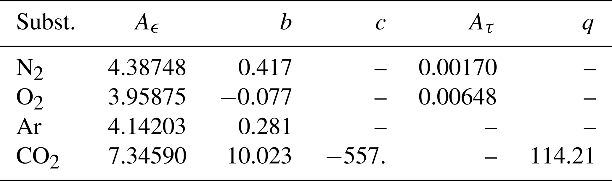
with d_m the molar density. The coefficients for the relevant substances are listed in Table 1; the values were provided with very high nominal accuracy.

It is noteworthy that the experimentally determined dielectric virial B_ϵ depends on the thermodynamic state, despite being proportional in principle to the molecular property α₀, which is often assumed constant. In AL11, the α₀ were indeed treated as constant. Part of the observed variation may reflect macroscopic effects such as uncertainties in the equation state used during data reduction in Schmidt and Moldover (2003). However, small physical variations of molecular polarizability with density or temperature are also plausible, due to intermolecular forces or molecular deformation, vibration or stretching.

Because measurements of Schmidt and Moldover (2003) are representative of highest current or foreseeable achievable accuracy for this type of experiment, we retain Eqs. (6) and (7) in the present study. This choice accepts that the molecular polarizabilities may not be strictly constant and that Table 1 captures these subtle effects. Including the tabulated coefficients preserves direct traceable connection between laboratory measurements and the refractivity model.

Table 1 Virial expression of the dielectric properties of the four leading constituents of dry air. Units of A_ϵ, b, and A_τ in cm³ mol⁻¹. Units of c and q in cm⁶ mol⁻².

Most dry-air constituents exhibit only very weak magnetic response. To verify the order of magnitude of the contributions, simple estimates of molecular magnetizability were used (Lide, 2001). The sole non-negligible contribution is from O₂, which is paramagnetic and possesses a comparatively large magnetic dipole moment ν_i (Aparicio and Laroche, 2011). Following AL11, a simplified model is adopted for all species except O₂, for which a more accurate expression from May et al. (2008) is used to represent the magnetic dipole ${\mathit{\nu }}_{{\mathrm{O}}_{\mathrm{2}}}$. The contribution of O₂ to Eq. (4) is:

$$\begin{array}{}\text{(8)}& \mathrm{4}\mathit{\pi }\left[{\mathit{\chi }}_{{\mathrm{O}}_{\mathrm{2}}}+{\displaystyle \frac{{\mathit{\nu }}_{{\mathrm{O}}_{\mathrm{2}}}^{\mathrm{2}}}{\mathrm{3}{k}_{B}T}}\right]=\left[-\mathrm{0.13}\times {\mathrm{10}}^{-\mathrm{9}}+{\displaystyle \frac{N_{\mathrm{A}}\cdot {\mathit{\mu }}_{\mathrm{0}}\cdot {\mathit{\mu }}_{\mathrm{m}}^{\mathrm{2}}}{\mathrm{3}{k}_{B}T}}\right]\end{array}$$

where ${\mathit{\mu }}_{\mathrm{0}}\equiv \mathrm{4}\mathit{\pi }\times {\mathrm{10}}^{-\mathrm{7}}$ N A⁻² is the vacuum permeability, and ${\mathit{\mu }}_{\mathrm{m}}=\sqrt{\mathrm{2}}\cdot \mathrm{2.00386}\cdot {\mathit{\mu }}_{\mathrm{B}}$ is the molecular magnetic moment, with ${\mathit{\mu }}_{\mathrm{B}}=\mathrm{9.274}\times {\mathrm{10}}^{-\mathrm{24}}$ J T⁻¹ the Bohr magneton. The comparatively large bulk permeability arises from the substantial magnetic dipole moment ${\mathit{\nu }}_{{\mathrm{O}}_{\mathrm{2}}}$, rather than a large molecular susceptibility ${\mathit{\chi }}_{{\mathrm{O}}_{\mathrm{2}}}$.

2.4 Water fraction

Water contributes to atmospheric refractivity primarily through its permanent electric dipole ${\mathit{\mu }}_{{\mathrm{H}}_{\mathrm{2}}\mathrm{O}}$, which is comparatively large among small molecules; by contrast most other air constituents are non-polar. The static polarizability ${\mathit{\alpha }}_{{\mathrm{H}}_{\mathrm{2}}\mathrm{O}}$, however, is similar in magnitude to that of the other major atmospheric species.

Because water is a major contributor to refractivity, and for consistency with AL11, several isotopologues are considered. These exhibit slightly different electric responses, mainly through variations in their molecular dipole moments. The overall effect on refractivity is minor, since the most abundant isotopologue (light water) comprises approximately 99.8 % of naturally occurring water. Although various processes in the hydrological cycle fractionate the isotopologues away from the global mean composition, this effect is neglected here, because it influences only a small fraction of water molecules. The isotopic fractions and microscopic properties used in this study follow AL11 and are based on IAPWS (2001) and Shostak et al. (1991).

The average molar mass of water is determined from the assumed isotopic composition and is taken to be constant across vapour, liquid and solid phases. The adopted value is m_w=18.01525.

Precipitated inclusions

Besides water vapour, atmospheric water also occurs in liquid (drops) and solid form (ice and snow). Under such conditions, condensed water contributes to the refractivity of the air matrix (Kursinski et al., 1997). This contribution may be represented by treating condensed water as small inclusions embedded in the air matrix (see Garnett, 1904), or, more symmetrically between phases, by an effective medium formulation that mixes multiple phases (Bruggeman, 1935). The resulting refractivity depends not only on the fraction of water present as hydrometeors but also on their shape and orientation.

Here, it is assumed that drops, ice crystals, and snowflakes may deviate from perfect sphericity, but only the simplest mode of asphericity is considered: rotational ellipsoids, with symmetry axes aligned with gravity.

Real hydrometeors are neither perfectly ellipsoidal, nor perfectly aligned as they fall. Random tilt of the principal axes is to be expected, and aerodynamic forcing (e.g. wind shear) may induce systematic tilt of the hydrometeors (known as canting). Moreover, drops, flakes and ice particles exhibit wide variability in size, shape, and orientation, with substantial spatial and temporal variability. Therefore, the present exploration of non-sphericity is not intended to be exhaustive; its purpose is to estimate the approximate effect on refractivity of the dominant main modes of asphericity. For the same reason, this model is not designed to retain high accuracy when hydrometeor concentrations are large, and the traceability link is not expected to remain robust in such cases. Although the accuracy of the nominal hydrometeor refractivity for a perfectly known distribution of hydrometeors should be better than 0.1 % of the hydrometeor contribution, the large variability in the atmosphere of hydrometeor concentration, size, shape, and orientation, suggests that use of this expression should allow a much larger uncertainty deriving from this variability. A safe value for this uncertainty in the presence of hydrometeors may be as large as 50 % of the estimated hydrometeor contribution.

An ellipsoidal dielectric inclusion embedded in a homogeneous matrix is polarizable and responds to an external test field (e.g. Stratton, 1941). The response includes a depolarizing field within the inclusion, which partially screens the interior from the applied field. The magnitude of this depolarization depends strongly on the object's shape and orientation relative to the field, and conversely, for a fixed shape and orientation of the object, the response depends on the direction of the test field with respect to the object.

All phases considered here – the matrix gas, liquid water, and to a very good approximation ice – are optically isotropic, responding identically to all electromagnetic polarizations. However, the geometric orientation of the hydrometeors may introduce anisotropy if they assume preferential orientations while falling. This constitutes a case of form anisotropy (Born and Wolf, 1999, Sect. 15.5.2). Falling drops deform into oblate shapes (Pruppacher and Beard, 1970), with the minor axis roughly vertical and two equal major axes lying horizontally. Ice and snow particles also tend to reorient.

Because depolarization depends on the relative alignment between the test field and the oblate hydrometeor, the effective medium consisting of the air matrix and the inclusions becomes anisotropic. Two principal configurations arise: the electric vector is aligned with the major axis of the hydrometeor, or with the minor axis (see Fig. 1). In the atmosphere, for horizontally propagating electromagnetic signals and vanishing canting, the electric vector aligns with the major axis for linear horizontal polarization (H, in Fig. 1), and with the minor axis for linear vertical polarization (V). All other combinations of drop orientation and polarization can be expressed as mixtures of these two cases.

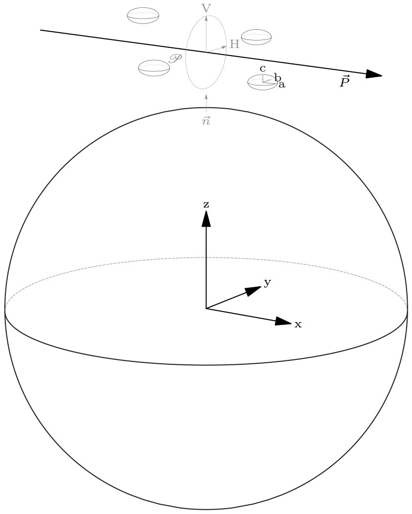
Figure 1 Scheme for a signal propagating along P, through the Earth's atmosphere. The signal finds flattened drops, of axes $a=b>c$ in its path. The electric field oscillates within the polarization plane 𝒫. Due to the symmetry of the drops, there is always in 𝒫 a direction H that lies inside the symmetry plane (a, b). Oscillations along this direction H meet the drops along their major axis. Oscillations in the perpendicular direction V meet the drops at some other angle, that depends on the elevation angle of the ray and the canting angle of the drops. In the case depicted, a horizontal ray and zero canting, V is oriented along the minor axis of the drops.

Interestingly, the dielectric response of the inclusions depends on the amount of condensed matter that they contain, as well as on their shape, but not directly on their size. Size and shape are correlated due to the fall (Pruppacher and Beard, 1970), and also through their association with meteorological variables such as rain rate. Because the aim is to characterise the optical properties of air, the independent variables are chosen to be those directly entering the refractivity expression – namely the amount of condensed water (in drops, ice or snow) and the particle shape –, rather than meteorological quantities that correlate with them.

Shape will be expressed as the axis ratio between the vertical (V) and horizontal (H) axes, denoted a_l for liquid drops and a_i for frozen particles. This ratio is 1 if they are spherical. Falling drops tend to become oblate, so typically a_l≤1.

A volume fraction η_l is occupied by liquid water, whose bulk electric permittivity many be represented by (Malmberg and Maryott, 1956):

$$\begin{array}{}\text{(9)}& {\log }_{\mathrm{10}}{\mathit{ϵ}}_{\mathrm{l}}=\mathrm{1.94315}-\mathrm{0.0019720}\cdot \left(T-\mathrm{273.15}K\right)\end{array}$$

These authors report an uncertainty of ${\mathit{\sigma }}_{{\mathit{ϵ}}_{\mathrm{l}}}=\mathrm{0.050}$. This permittivity is very large, and produces large depolarization fields in the drops, strongly screening the molecules inside from the test field. Since the overall contribution of liquid water to air's refractivity is small, this expression is here considered to be sufficiently accurate.

Similarly, a volume fraction η_i is occupied by ice or snow, with axis ratio a_i, which may differ from unity. For ice, the electric permittivity from Mätzler and Wegmüller (1987) is chosen here:

$$\begin{array}{}\text{(10)}& {\mathit{ϵ}}_{\mathrm{i}}=\mathrm{3.1884}+\mathrm{9.1}\times {\mathrm{10}}^{-\mathrm{4}}\cdot \left(T-\mathrm{273.15}K\right)\end{array}$$

where they estimate the error to be ${\mathit{\sigma }}_{{\mathit{ϵ}}_{\mathrm{i}}}=\mathrm{0.0050}$. This permittivity is also large, though less than that of liquid water. This expression is considered adequate, since even under extreme conditions (e.g. intense hail) ice contributes only a small fraction air's refractivity.

In summary, the independent variables introduced here are the precipitated mass of liquid and solid water per unit volume of air, ρ_l and ρ_i. These correspond to the liquid water content (LWC) and ice water content (IWC), typically ranging $\mathrm{0}\le {\mathit{\rho }}_{\mathrm{l}}<{\mathrm{10}}^{-\mathrm{2}}$ and $\mathrm{0}\le {\mathit{\rho }}_i\le \mathrm{4}\times {\mathrm{10}}^{-\mathrm{3}}$, in kg m⁻³. Axis ratios (vertical/horizontal) for liquid and solid ellipsoids a_l and a_i have been considered between 0.5 and 1.25.

2.5 Multiphase model

Air is represented here as an effective medium composed of three phases: a gas matrix occupying most of the volume, and possibly liquid and ice phases present as small inclusions. Their respective volume fractions are η_g, η_l, and η_i, which are subject to ${\mathit{\eta }}_g+{\mathit{\eta }}_l+{\mathit{\eta }}_i=\mathrm{1}$, and typically ${\mathit{\eta }}_g\gg {\mathit{\eta }}_l+{\mathit{\eta }}_i$.

The phases have permittivities ϵ_g, ϵ_l, and ϵ_i. These are assumed to be known: ϵ_g from the microscopic gas-phase model described above, and ϵ_l and ϵ_i from published measurements (Malmberg and Maryott, 1956; Mätzler and Wegmüller, 1987). At scales large enough for the mixture to appear homogeneous, the ensemble of the gas matrix and embedded inclusions exhibits an effective permittivity ϵ_r, which we aim to determine.

Following Choy (1999) (and references therein), the effective medium corresponds to a certain average of the different phases k. The average can be obtained by solving:

$$\begin{array}{}\text{(11)}& \sum _k{\mathit{\eta }}_k\left({\displaystyle \frac{{\mathit{ϵ}}_k-{\mathit{ϵ}}_{\mathrm{r}}}{{\mathit{ϵ}}_k+p_k^i\cdot {\mathit{ϵ}}_{\mathrm{r}}}}\right)=\mathrm{0}\end{array}$$

which is approximately a volume-weighted average. Here $p_k^i=\mathrm{1}/P_k^i-\mathrm{1}$ is a shape factor that depends on the depolarizing factor $P_k^i$. The depolarizing factors describe the geometric exposure of the material inside the inclusions of phase k, to a test field oriented along direction i direction, and satisfy, for each phase k: ${\sum }_{i\in (x,y,z)}{P}_k^i=\mathrm{1}$. Because the depolarization depends on both the shape of the inclusions and their relative orientation relative to the test field (Stratton, 1941), the effective dielectric response ϵ_r is direction-dependent. Thus, instead of a single scalar permittivity, the model yields directional components ${\mathit{ϵ}}_{\mathrm{r}}^i$, corresponding for example to different polarization states of the test field.

A rearrangement of Eq. (11), using the dominance of the gas phase and allowing for direction-dependent effective permittivities ${\mathit{ϵ}}_{\mathrm{r}}^i$, gives:

$$\begin{array}{}\text{(12)}& {\mathit{ϵ}}_{\mathrm{r}}^i={\mathit{ϵ}}_g+{\displaystyle \frac{{\mathit{ϵ}}_g+p_g^i\cdot {\mathit{ϵ}}_{\mathrm{r}}^i}{{\mathit{\eta }}_g}}\sum _{k\ne g}{\mathit{\eta }}_k\cdot {\displaystyle \frac{{\mathit{ϵ}}_k-{\mathit{ϵ}}_{\mathrm{r}}^i}{{\mathit{ϵ}}_k+p_k^i\cdot {\mathit{ϵ}}_{\mathrm{r}}^i}}\end{array}$$

As noted in Sect. (2.1), ϵ_g is implicitly defined and depends weakly on the dielectric response of the surrounding medium, previously denoted ϵ_r, but which becomes direction-dependent ${\mathit{ϵ}}_{\mathrm{r}}^i$ in the presence of hydrometeors. The nonlinearities in Eq. (2), for ϵ_g, and in Eq. (12), for ${\mathit{ϵ}}_{\mathrm{r}}^i$, suggest an iterative solution as the most appropriate approach. Starting with an initial guess ${\mathit{ϵ}}_{\mathrm{r}}^i=\mathrm{1}$ leads to rapid convergence.

The simplest inclusions are small spheres, representative for example of small droplets. Their symmetry implies $P^i=\mathrm{1}/\mathrm{3}$ for all i. Here, the possible inclusions are generalized to rotational ellipsoids whose axis of rotation is nearly vertical, possibly with some canting. Because particles fall under gravity, the two quasi-horizontal directions are expected to be equivalent. The degree of asphericity is represented by the axial ratio a, defined as the ratio of the quasi-vertical to quasi-horizontal axes. Typical atmospheric values lie between 0.5–1 (Pruppacher and Beard, 1970). Exact closed-form expressions exist for the depolarization factors Pⁱ of arbitrary ellipsoids (e.g. Landau et al., 1984), but given the variability of real hydrometeors in shape and orientation, a simpler but accurate approximation is sufficient.

We therefore use two depolarization factors for each inclusion type: P_v for test fields along the quasi-vertical axis (the axis of symmetry), and P_h for fields in the quasi-horizontal plane. These must satisfy $P_{\mathrm{v}}+\mathrm{2}\cdot P_{\mathrm{h}}=\mathrm{1}$. The following approximate expressions, proposed by Jones and Friedman (2000), satisfy the closure relations and reproduce the limiting behaviours:

$$\begin{array}{}\text{(13)}& P_{\mathrm{v}}={\displaystyle \frac{\mathrm{1}}{\mathrm{1}+\mathrm{1.6}\cdot a+\mathrm{0.4}\cdot a^{\mathrm{2}}}}\end{array}$$

and $P_{\mathrm{h}}=\mathrm{0.5}\cdot \left(\mathrm{1}-P_{\mathrm{v}}\right)$. For spherical hydrometeors (a=1), these reduce to $P_{\mathrm{v}}=P_{\mathrm{h}}=\mathrm{1}/\mathrm{3}$. For aligned oblate spheroids, as drops, where a<1, they satisfy $P_{\mathrm{v}}>\mathrm{1}/\mathrm{3}>P_{\mathrm{h}}$.

2.6 Axial ratios

Liquid and frozen hydrometeors (drops, ice particles, and snowflakes) have been treated as inclusions within an effective-medium, the matrix being the gas phase of air, which includes dry air and water vapour. The effective index of refraction of the mixture depends primarily on mass fraction of each phase (gas, liquid, and ice), and the dielectric properties of those phases, with an additional, weaker dependence on the shapes of the inclusions. Even if each individual phase is dielectrically isotropic, preferential hydrometeor shapes introduce geometric anisotropy into the mixture, resulting in a macroscopically anisotropic optical response.

When liquid water and snow particles are preferentially aligned around a quasi-vertical direction, two refraction indices must be evaluated, one for electric test fields along the alignment direction (“vertical”), and another for fields perpendicular to it (“horizontal”). While the alignment need not be perfectly vertical or horizontal because of canting, these terms remain convenient. These resulting refraction indices depend on the amount of precipitated water, its thermodynamic phase, and the mean axial ratios of the inclusions, but not directly on particle size. Indirectly, however, size does influence the axial ratios: larger raindrops and higher rain rates are associated with more pronounced flattening (see Pruppacher and Pitter, 1971; Beard and Chuang, 1987; Beard et al., 2010, and references therein).

Numerous studies of raindrop shape indicate that liquid hydrometeors can be represented as oblate spheroids with axial ratios between 0.5 and 1. Several empirical relationships have been proposed linking axial ratio, drop size, and rain rate. A simple, order of magnitude example, Pruppacher and Beard (1970) suggests:

$$\begin{array}{}\text{(14)}& a_{\mathrm{l}}=min(\mathrm{1.030}-\mathrm{0.124}{r}_{\mathrm{0}},\mathrm{1})\end{array}$$

where r₀ is the drop-equivalent (volume-based) radius. In this study, however, we focus solely on the optical coupling between drops and the electromagnetic field, which does not depend explicitly on drop size.

Ice particles are not flexible to adjust their shapes as they fall, but they do exhibit preferential orientation. Depending on the specific hydrometeor type (pellets, hail, crystals, etc.), both oblate and prolate forms are commonly observed. For the purposes of this work, limited to only the axial ratio, we explore a representative range of $\mathrm{0.5}<a_i<\mathrm{1.25}$.

2.7 Approximation to the evolution of composition

Long-term atmospheric composition records show that, beyond seasonal patterns, the atmospheric fraction of CO₂ has been steadily increasing, while the fraction of O₂ has been decreasing (e.g. Keeling et al., 2001). Both trends reflect carbon-oxidation processes. The quantitative relationship between the two is not fixed, and depends on the stoichiometry of oxidation processes, as well as on additional sources and sinks of carbon and oxygen.

The predominant forms of carbon oxidation would suggest that substitution of O₂ to CO₂ in air approximately a 1:1 molar ratio, implying that the molar sum of O₂ and CO₂ should remain nearly constant. This behaviour is often observed in short-term laboratory studies (e.g. Picard et al., 2008), and in urban environments (e.g. Keeling, 1988). However, long-term background observations of molar fraction in well-mixed non-urban areas, show that the decline in O₂ is significantly larger – by roughly a factor of two, (Keeling et al., 2001) – than the increase of CO₂. This disparity is interpreted as evidence that a substantial fraction of the newly produced atmospheric CO₂ is transferred to land and ocean reservoirs, where it accumulates – particularly in dissolved form within the oceans – while atmospheric O₂ experiences comparatively limited exchange (Manning and Keeling, 2006).

Given the availability of multi-decadal background observations from numerous stations (see Keeling et al., 2001; Keeling, 2015a), we may produce fits to the composition over recent decades. A quadratic function of time provides a good fit to the deseasonalized record from 1958 to the present. Because there is a significant latitudinal gradient, a hemispheric asymmetry term is included, proportional to the sine of latitude λ. Since the period of interest for the present study corresponds to the availability of GNSS observations (approximately 1994–present), time is expressed relative to the year 2000, as $y_{\mathrm{2000}}=y-\mathrm{2000}$. The residuals of the fit are small, suggesting that expression can reasonably be extrapolated into the near future.

$$\begin{array}{}\text{(15)}& \begin{array}{rl}{x}_{{\mathrm{CO}}_{\mathrm{2}}}(y,\mathit{\lambda })& ={\mathrm{10}}^{-\mathrm{6}}\cdot [\mathrm{368.625}+\mathrm{1.798}\cdot y_{\mathrm{2000}}+\mathrm{0.0118}\\ & \cdot y_{\mathrm{2000}}^{\mathrm{2}}+\mathrm{2.224}\cdot \sin \left(\mathit{\lambda }\right)]\end{array}\end{array}$$

which captures both a linear trend and a measurable acceleration.

Oxygen is not measured by Keeling et al. (2001) in absolute units, but relative to a reference sample. The deseasonalized trends from this relative dataset (Keeling, 2015b) constrain the rate of decline, its acceleration, and the latitudinal dependence. The absolute level is set using measurements by Tohjima et al. (2005), who report $x_{{\mathrm{O}}_{\mathrm{2}}}=\mathrm{0.209392}\pm \mathrm{3}$, at the year 2000 and at latitude 24N. The constant term in Eq. (16) is chosen to reproduce that value, with the remaining terms reproduce the relative measurements:

$$\begin{array}{}\text{(16)}& \begin{array}{rl}{x}_{{\mathrm{O}}_{\mathrm{2}}}(y,\mathit{\lambda })& ={\mathrm{10}}^{-\mathrm{6}}\cdot [\mathrm{209393}-\mathrm{3.953}\cdot y_{\mathrm{2000}}-\mathrm{0.0363}\\ & \cdot y_{\mathrm{2000}}^{\mathrm{2}}-\mathrm{3.064}\cdot \sin \left(\mathit{\lambda }\right)]\end{array}\end{array}$$

Both fits are intended to capture the long-term background evolution. These measurements reflect well-mixed tropospheric air, which becomes homogenized over a time scale of a few months. Stratospheric air exchanges more slowly with the troposphere, leading to detectable differences in CO₂ concentration (e.g. Georgii and Jost, 1969) and to a typical lag of about 4 years in stratospheric CO₂ relative to the deseasonalized tropospheric mean. This lag varies with latitude and altitude, typically between 1–6 years (Andrews et al., 2001). A further refinement could incorporate the seasonal cycle in the troposphere – especially pronounced in the northern hemisphere and reaching a few ppm – but for the purposes of this study the above expressions are sufficiently accurate. In particular, the absolute abundance of O₂ is not known to within better than about 3 ppm, comparable to the amplitude of the seasonal cycle.

3 Proposed expression

An ansatz analogous to the one proposed in Aparicio and Laroche (2011) is adopted in this study. Relative to that earlier formulation, two principal modifications are introduced. First, the main dry-air term is no longer treated as constant, because the atmospheric composition is not assumed to be static. Although the resulting dependence is small for compositions observed in recent decades, it is included here to assess the long-term signature of composition changes in refractivity. Second, additional terms are incorporated to represent the contributions of precipitated water. These are known to be moderately small (Kursinski et al., 1997), but particular attention is paid in order to explore the optical anisotropy that they may develop. The proposed ansatz is:

$$\begin{array}{}\text{(17)}& {\displaystyle }N\equiv (n-\mathrm{1})\cdot {\mathrm{10}}^{\mathrm{6}}=N_{\mathrm{0}}\cdot \left(\mathrm{1}+{\displaystyle \frac{{\mathrm{10}}^{-\mathrm{6}}}{\mathrm{6}}}{N}_{\mathrm{0}}\right)\text{(18)}& {\displaystyle }{N}_{\mathrm{0}}=\left[q_{\mathrm{1}}\left(x_{{\mathrm{O}}_{\mathrm{2}}},x_{{\mathrm{CO}}_{\mathrm{2}}}\right)+q_{\mathrm{2}}\cdot \mathit{\tau }\right]{\mathit{\rho }}_{\mathrm{d}}+\text{(19)}& {\displaystyle }\left[q_{\mathrm{3}}+q_{\mathrm{4}}\cdot \mathit{\tau }\right]{\mathit{\rho }}_{\mathrm{w}}+\text{(20)}& {\displaystyle }{q}_{\mathrm{5}}\cdot f_{\mathrm{l}}(a_{\mathrm{l}};p)\cdot {\mathit{\rho }}_{\mathrm{l}}+\text{(21)}& {\displaystyle }{q}_{\mathrm{6}}\cdot f_i(a_i;p)\cdot {\mathit{\rho }}_i\end{array}$$

where the refractivity N depends on the amount of matter per unit volume in each component: dry air ρ_d, water vapour ρ_w, liquid water ρ_l, and frozen water ρ_i. Refractivity also depends on the absolute temperature T through $\mathit{\tau }=\mathrm{273.15}K/T-\mathrm{1}$. The function q₁, which is nearly constant, is assumed to take the form:

$$\begin{array}{}\text{(22)}& q_{\mathrm{1}}\left(x_{{\mathrm{O}}_{\mathrm{2}}},x_{{\mathrm{CO}}_{\mathrm{2}}}\right)=q_{\mathrm{10}}+q_{\mathrm{11}}\cdot \left(x_{{\mathrm{O}}_{\mathrm{2}}}-\mathrm{0.2095}\right)+q_{\mathrm{12}}\cdot x_{{\mathrm{CO}}_{\mathrm{2}}}\end{array}$$

where the first term represents the average composition of dry air, in the limit of vanishing CO₂. The second accounts for small deviations of the O₂ molar fraction relative to the reference value of $x_{{\mathrm{O}}_{\mathrm{2}}}=\mathrm{0.2095}$, close to present-day conditions. The third term represents the contribution of CO₂. A linear dependence is considered sufficient for both the second and third terms, because variations of O₂ around the reference value are small, and CO₂ remains a trace constituent.

Since Eq. (18) is expressed in terms of density, and its conversion to pressure is frequently required, we provide the corresponding expression for the mean molar mass of dry air that is consistent with the assumed composition.

$$\begin{array}{}\text{(23)}& {\displaystyle }{m}_d\left(x_{{\mathrm{O}}_{\mathrm{2}}},x_{{\mathrm{CO}}_{\mathrm{2}}}\right)=m_{d\mathrm{0}}+m_{d\mathrm{1}}\cdot \left(x_{{\mathrm{O}}_{\mathrm{2}}}-\mathrm{0.2095}\right)+m_{d\mathrm{2}}\cdot x_{{\mathrm{CO}}_{\mathrm{2}}}\end{array}$$

The polarization functions are modelled as quadratic functions of the axial ratio and depend on the linear polarization state p, which may be aligned with the rotation axis of the hydrometeor ellipsoids (denoted vertical or V), or perpendicular to it (horizontal, H), see Fig. 1). For liquid inclusions:

$$\begin{array}{}\text{(24)}& {\displaystyle }{f}_{\mathrm{l}}(a_{\mathrm{l}};V)=\mathrm{1}+c_{\mathrm{1}V}\cdot (a_{\mathrm{l}}-\mathrm{1})+c_{\mathrm{2}V}\cdot (a_{\mathrm{l}}-\mathrm{1}{)}^{\mathrm{2}}\text{(25)}& {\displaystyle }{f}_{\mathrm{l}}(a_{\mathrm{l}};H)=\mathrm{1}+c_{\mathrm{1}H}\cdot (a_{\mathrm{l}}-\mathrm{1})+c_{\mathrm{2}H}\cdot (a_{\mathrm{l}}-\mathrm{1}{)}^{\mathrm{2}}\end{array}$$

and solid:

$$\begin{array}{}\text{(26)}& {\displaystyle }{f}_i(a_i;V)=\mathrm{1}+d_{\mathrm{1}V}\cdot (a_i-\mathrm{1})+d_{\mathrm{2}V}\cdot (a_i-\mathrm{1}{)}^{\mathrm{2}}\text{(27)}& {\displaystyle }{f}_i(a_i;H)=\mathrm{1}+d_{\mathrm{1}H}\cdot (a_i-\mathrm{1})+d_{\mathrm{2}H}\cdot (a_i-\mathrm{1}{)}^{\mathrm{2}}\end{array}$$

The closure relation for the depolarization coefficients imposes constraints between the two polarizations, namely: $c_{\mathrm{1}V}+\mathrm{2}\cdot c_{\mathrm{1}H}=\mathrm{0}$, and $d_{\mathrm{1}V}+\mathrm{2}\cdot d_{\mathrm{1}H}=\mathrm{0}$.

3.1 Fit to a user expression

The coefficients introduced above are determined by constructing a large ensemble of physical conditions – spanning pressure, temperature, moisture, dry air composition, and hydrometeor shape – that reflects a broad range of realistic atmospheric states.

Pressures are selected to represent conditions from the surface to the mid-stratosphere. Surface temperatures range from −60 to 40 °C, and are extrapolated to upper-air temperatures using typical lapse rates (NOAA et al., 1976). Water vapour is varied from zero up to 25 % above saturation at the local conditions. To avoid unrealistically moist stratospheric states, a constraint is imposed to prevent the water fraction from increasing with altitude. In supersaturated cases, water vapour is capped at the saturation density, with any excess assigned to hydrometeors. Hydrometeor mass therefore reaches up to 25 % of the saturation density of the local saturation vapour density, partitioned liquid or solid according to temperature.

Carbon dioxide concentrations range from 300 and 450 ppm, and the O₂ molar fraction from 0.209 and 0.210. Axial ratios (vertical/horizontal) of hydrometeor ellipsoids span the interval 0.5–1.25.

The full ensemble comprises more than 150 000 atmospheric states. For each state, the microphysical model is used to compute the refractivity for both linear polarizations, and the molar mass of dry air is evaluated.

To ensure numerical stability, the fitting procedure is carried out in two stages. In the first stage, all coefficients not related to hydrometeor asphericity are adjusted. This stage involves the expressions between Eqs. (17) and (23), and determines coefficients q₁ to q₆, including q₁₀ to q₁₂, and m_d0 to m_d2. Only the subset of conditions that contain either no hydrometeors, or hydrometeors of spherical shape is included. This first fit yields the following expression:

$$\begin{array}{}\text{(28)}& {\displaystyle }{N}_{\mathrm{0}}=\left[q_{\mathrm{1}}(x_{{\mathrm{O}}_{\mathrm{2}}},x_{{\mathrm{CO}}_{\mathrm{2}}})+\mathrm{0.097}\cdot \mathit{\tau }\right]{\mathit{\rho }}_{\mathrm{d}}+\text{(29)}& {\displaystyle }\left[\mathrm{6703.497}+\mathrm{6393.484}\cdot \mathit{\tau }\right]{\mathit{\rho }}_{\mathrm{w}}+\text{(30)}& {\displaystyle }\mathrm{1447.827}\cdot f_{\mathrm{l}}(a_{\mathrm{l}};p)\cdot {\mathit{\rho }}_{\mathrm{l}}+\text{(31)}& {\displaystyle }\mathrm{686.944}\cdot f_i(a_i;p)\cdot {\mathit{\rho }}_i\end{array}$$

with refractivity expressed in N-units, densities in kg m⁻³, and $\mathit{\tau }=(\mathrm{273.15}K/T-\mathrm{1})$. The function q₁ is determined from the first-stage fit to be:

$$\begin{array}{}\text{(32)}& \begin{array}{rl}{q}_{\mathrm{1}}(x_{{\mathrm{O}}_{\mathrm{2}}},x_{{\mathrm{CO}}_{\mathrm{2}}})& =\mathrm{222.637}-\mathrm{51.817}\cdot \left(x_{{\mathrm{O}}_{\mathrm{2}}}-\mathrm{0.2095}\right)\\ & +\mathrm{30.266}\cdot x_{{\mathrm{CO}}_{\mathrm{2}}}\end{array}\end{array}$$

To preserve the intended accuracy of the formulation, the expression must be used together with a consistent relationship between mass and molar density, and therefore with a consistent value of the mean molar mass of dry air, which is likewise obtained from the fit:

$$\begin{array}{}\text{(33)}& \begin{array}{rl}{m}_d(x_{{\mathrm{O}}_{\mathrm{2}}},x_{{\mathrm{CO}}_{\mathrm{2}}})& =\mathrm{28.95949}+\mathrm{3.985}\cdot \left(x_{{\mathrm{O}}_{\mathrm{2}}}-\mathrm{0.2095}\right)\\ & +\mathrm{15.996}\cdot x_{{\mathrm{CO}}_{\mathrm{2}}}\end{array}\end{array}$$

As noted in Sect. 2.4, the molar mass of water is taken as constant in this model, with value:

$$\begin{array}{}\text{(34)}& m_w=\mathrm{18.01525}\end{array}$$

With all these coefficients fixed, a second fit is performed to determine the shape-dependent and polarization-dependent functions, now extending the physical conditions to include aspherical hydrometeors. For liquid hydrometeors, the functions for the two linear polarizations are:

$$\begin{array}{}\text{(35)}& {\displaystyle }{f}_{\mathrm{l}}(a_{\mathrm{l}};V)=\mathrm{1}+\mathrm{0.743}\cdot (a_{\mathrm{l}}-\mathrm{1})+\mathrm{0.043}\cdot (a_{\mathrm{l}}-\mathrm{1}{)}^{\mathrm{2}}\text{(36)}& {\displaystyle }{f}_{\mathrm{l}}(a_{\mathrm{l}};H)=\mathrm{1}-\mathrm{0.371}\cdot (a_{\mathrm{l}}-\mathrm{1})+\mathrm{0.753}\cdot (a_{\mathrm{l}}-\mathrm{1}{)}^{\mathrm{2}}\end{array}$$

and for ice:

$$\begin{array}{}\text{(37)}& {\displaystyle }{f}_i(a_i;V)=\mathrm{1}+\mathrm{0.330}\cdot (a_i-\mathrm{1})-\mathrm{0.125}\cdot (a_i-\mathrm{1}{)}^{\mathrm{2}}\text{(38)}& {\displaystyle }{f}_i(a_i;H)=\mathrm{1}-\mathrm{0.165}\cdot (a_i-\mathrm{1})+\mathrm{0.215}\cdot (a_i-\mathrm{1}{)}^{\mathrm{2}}\end{array}$$

By construction, this second fit satisfies the closure condition on the coefficients that are linear in (a−1).

Across the full range of atmospheric conditions considered – spanning and exceeding those expected in practice – the fitted expressions reproduce the microphysical model with an average absolute residual of 0.0016 %, and a maximum residual of 0.009 %. This performance exceeds both the estimated accuracy of the microphysical model and the intended accuracy of this work. The overall accuracy is therefore limited solely by the microphysical model itself, not by the fitting procedure.

3.2 A time-dependent form of the proposed expression

The fit to the microphysical model spans a range of physical conditions and dry-air compositions representative of recent decades and the foreseeable future. Two composition parameters are retained as independent variables, appearing in the functions $q_{\mathrm{1}}\left(x_{{\mathrm{O}}_{\mathrm{2}}},x_{{\mathrm{CO}}_{\mathrm{2}}}\right)$ and $m_d\left(x_{{\mathrm{O}}_{\mathrm{2}}},x_{{\mathrm{CO}}_{\mathrm{2}}}\right)$. Because measurements exist for both quantities, and can be described, for example, by the functions introduced in Sect. 2.7, it is possible to further reduce q₁ and m_d to explicit functions of time. In this section, we illustrate this procedure using Eqs. (15) and (16). The user must judge whether adopting only the long-term trends of O₂ and CO₂ is sufficient, or whether latitudinal, seasonal, or altitude variations should also be incorporated.

Using the temporal fits of molar fractions yields:

$$\begin{array}{}\text{(39)}& \begin{array}{rl}{q}_{\mathrm{1}}\left(x_{{\mathrm{O}}_{\mathrm{2}}},x_{{\mathrm{CO}}_{\mathrm{2}}}\right)& \simeq q_{\mathrm{1}}\left(y\right)=\mathrm{222.654}+\mathrm{0.000259}\cdot y_{\mathrm{2000}}\\ & +\mathrm{2.24}\times {\mathrm{10}}^{-\mathrm{6}}\cdot y_{\mathrm{2000}}^{\mathrm{2}}\end{array}\end{array}$$

and

$$\begin{array}{}\text{(40)}& \begin{array}{rl}{m}_d\left(x_{{\mathrm{O}}_{\mathrm{2}}},x_{{\mathrm{CO}}_{\mathrm{2}}}\right)& \simeq m_d\left(y\right)=\mathrm{28.96496}+\mathrm{1.30}\times {\mathrm{10}}^{-\mathrm{5}}\\ & \cdot y_{\mathrm{2000}}+\mathrm{4.41}\times {\mathrm{10}}^{-\mathrm{8}}\cdot y_{\mathrm{2000}}^{\mathrm{2}}\end{array}\end{array}$$

A time-dependent user expression is therefore obtained by combining Eqs. (28), (39) and (40).

A particularly relevant limit is that of pure dry air, often invoked in a variety of atmospheric applications:

$$\begin{array}{}\text{(41)}& N_{\mathrm{dry}}=\left[q_{\mathrm{1}}(x_{{\mathrm{O}}_{\mathrm{2}}},x_{{\mathrm{CO}}_{\mathrm{2}}})+\mathrm{0.097}\cdot \mathit{\tau }\right]{\mathit{\rho }}_{\mathrm{d}}\end{array}$$

It is useful to compare this expression with others commonly found in the literature, such as the classical form in Smith and Weintraub (1953):

$$\begin{array}{}\text{(42)}& N_{\mathrm{dry}}^a=k_{\mathrm{1}}{\displaystyle \frac{P}{T}}\end{array}$$

in which the parameter here labeled k₁ is not exactly a constant, but is modulated by the compressibility factor Z, for instance in Thayer (1974):

$$\begin{array}{}\text{(43)}& N_{\mathrm{dry}}^{Th\mathrm{74}}={\displaystyle \frac{\mathrm{77.60}}{Z}}{\displaystyle \frac{P}{T}}\end{array}$$

An accurate expression of the compressibility factor from (Picard et al., 2008) is used in the microphysical model. For the purposes of this section, however, it is sufficient to adopt the approximation:

$$\begin{array}{}\text{(44)}& Z_{\mathrm{app}}\approx \mathrm{1}-P\cdot \left(\mathrm{5.789}\times {\mathrm{10}}^{-\mathrm{9}}-\mathrm{3.512}\times {\mathrm{10}}^{-\mathrm{8}}\cdot \mathit{\tau }\right)\end{array}$$

with P in pascals. In the dry-air limit – appropriate for instance to the stratosphere, and to good approximation, in dry tropospheric air where deviations of Z from unity remain small –, the following holds:

$$\begin{array}{}\text{(45)}& k_{\mathrm{1}}={\displaystyle \frac{q_{\mathrm{1}}\cdot m_d}{\mathrm{10}\cdot RZ}}\simeq {\displaystyle \frac{\mathrm{77.5655}}{Z_{\mathrm{app}}}}+\mathrm{1.25}\cdot {\mathrm{10}}^{-\mathrm{4}}\cdot y_{\mathrm{2000}}+\mathrm{8.98}\cdot {\mathrm{10}}^{-\mathrm{7}}\cdot y_{\mathrm{2000}}^{\mathrm{2}}\end{array}$$

If we compare this with the formulation of AL11, which used a composition approximately representative of 2010, we would obtain here $k_{\mathrm{1}}\simeq \frac{\mathrm{77.5668}}{Z_{\mathrm{app}}}$, against an asymptotic low-density value of AL11 is $k_{\mathrm{1}}\simeq \frac{\mathrm{77.575}}{Z_{\mathrm{app}}}$. For the ROMEX experiment, which is performed with measurements from 2022, the asymptotic low-density behaviour is $k_{\mathrm{1}}\simeq \frac{\mathrm{77.5687}}{Z_{\mathrm{app}}}$. The difference between AL11 and the current model arises primarily from the use of a slightly different fit in Schmidt and Moldover (2003) to the same underlying laboratory data for dielectric gas properties, and also to a different choice of atmospheric conditions to reduce the microphysical model to a practical expression. Both formulations remain compatible within their intended target of accuracy. Among these available dielectric fits, the expression adopted here is preferred because it provides uncertainty estimates for all coefficients, thereby enabling traceability of the error budget back to the laboratory measurements, which is one of the purposes of this study.

3.3 Double refraction

The refractivity model in Eq. (28) describes an isotropic medium in the absence of hydrometeors, or when these are spherical (a_lρ_l=0 and a_iρ_i=0). In contrast, aligned aspherical hydrometeors introduce anisotropy, yielding different refractivities for test fields (i.e. linear polarizations) aligned with the major and minor axes of the hydrometeors. In this section we estimate, at an order of magnitude level, the resulting impact on wave propagation in the two polarizations, focusing on the geometry of a radio occultation.

Because GNSS applications are a primary motivation for the present formulation, it is useful to recall that the carrier of a standard GPS signal is, upon emission, right-hand circularly polarized. This can be viewed as the superposition of two orthogonal linearly polarized components, one of them delayed by a quarter wavelength with respect to the other.

The electric-field polarization is defined in the plane perpendicular to the local Poynting vector P. In an occultation (a limb observation) this vector is approximately horizontal, and the normal plane can be described with a basis of a horizontal and a vertical orthogonal unit vectors, which align to the major and minor axes of the hydrometeors; see Fig. 1. In contrast, in a quasi-zenithal observation, as with Ground-Based GNSS receivers, P is aligned to the hydrometeors' rotation axis. The plane perpendicular to P is then symmetric concerning Eq. (28), and all polarizations behave as the H component in that equation, with identical refractivity.

Polarization components in a GNSS observation may therefore experiance different refractive indices. In the limb-viewing geometry, the plane of the electric field contains a subspace aligned with a horizontal axis of the hydrometeors. Electic activity in this subspace senses a refraction index n_H, a component referred to as ordinary (Born and Wolf, 1999, Sect. 15.3.2). Activity in the perpendicular subspace of the same plane, which is aligned with the vertical minor axis V, senses instead n_V, a component referred as extraordinary.

If both polarizations encounter the same refractive index, they follow identical trajectories and retain their relative phase delay. If instead one polarization experiences a higher refractive index, two effects arise:

• a modification of the relative delay between the two components, and

• a differential geometric propagation path (i.e. double refraction) between transmitter and receiver.

Although both effects vanish in many atmospheris situations (no hydrometeors, or hydrometeors of spherical average shape), we estimate here the magnitude they may reach under extreme but still realistic conditions during an occultation in the low troposphere:

• a vertical/horizontal axis ratio a_l=0.5 for liquid or a_i=1.25 for ice, representative of large raindrops (Pruppacher and Beard, 1970) and hail (Knight and Knight, 2005);

• maximum precipitated densities (FAA, 2016) of ${\mathit{\rho }}_{\mathrm{l}}={\mathrm{10}}^{-\mathrm{2}}$ kg m⁻³ for rain and ${\mathit{\rho }}_i=\mathrm{4}\times {\mathrm{10}}^{-\mathrm{3}}$ kg m⁻³ for frozen hydrometeors;

• a horizontal propagation distance of 50 km under these conditions (Kessler, 1975, and references therein).

The rain case suggests a liquid contribution to the total refractivity (in N-units) of about N_l≈15, with a large asymmetry between polarizations: N_lH≈20 and N_lV≈10. Here, N_lH>N_lV, because the drops are substantially oblate (Pruppacher and Beard, 1970). In the hail case, contribution to refractivity is smaller <3, with moderate asymmetry, N_iH≈2.7 and N_iV≈3.0, i.e. N_iH<N_iV, for the assumed prolateness.

Accumulated over the 50 km of horizontal propagation, the refractivity asymmetry yields an optical path difference (at equal geometric paths) of $\mathrm{\Delta }{L}_{H-V}\approx \mathrm{0.5}\mathrm{m}$ (H minus V polarizations) for the rain case, and $\mathrm{\Delta }{L}_{H-V}\approx -\mathrm{0.015}\mathrm{m}$ for the hail case. Rain is both more refractive and can reach larger extreme mass densities than ice, but even in these extreme cases the resulting differences remain moderate. These path differences are detectable by receivers capable of discriminating both polarizations, see for instance (Cardellach et al., 2015; Padullés et al., 2020, 2023, 2025; Talpe et al., 2025).

In addition to producing a differential optical path length, a difference in refractivity between the two polarization components also causes their propagation paths to split (birefringence). Under typical occultation geometry, and given an assumed typical background atmospheric gradient, the rain example implies that the horizontal polarization component propagates above the vertical polarization, as the horizontal component encounters a larger refractivity at the same altitude, in this example by about 200 m. The example is chosen as an extreme case, derived from large but still realistic rain density, sustained over a large geographic area (infrequent under intense rain). Smaller values of the tangent point split, of 10s of meters, should be more common but still detectable. At fixed reception time, an occulting signal containing both polarizations (e.g. a circularly polarized GPS signal) would therefore exhibit different tangent point heights in each polarization, separated by roughly this amount. This is illustrated in Fig. 2.

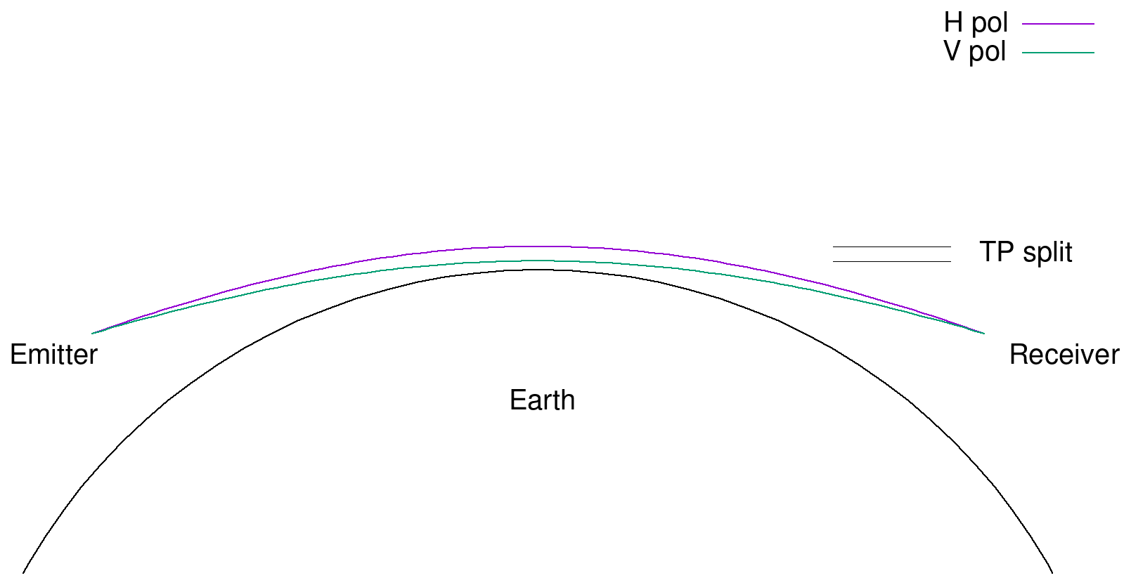
Figure 2 Schematic representation of the tangent point (TP) separation between polarizations in the case of oblate hydrometeors, typical of rain. In the path between two Earth-orbiting satellites, the horizontal polarization component (H) senses a higher refractive index, and follows a longer (higher) path than the vertical polarization (V). The scale is exaggerated for clarity.

During the occultation scan, the tangent point reaches a given altitude with a time delay between the two components; with a typical vertical scan rate of the order of 1 km s⁻¹, the delay reaches about 0.2 s in this extreme scenario – still smaller than the Fresnel diameter. The reduction of scan rate in the low atmosphere would favor the detectability. In the hail example case, the path split is correspondingly smaller, about 10 m, and the order of the polarizations is reversed: the vertical component lies above the horizontal, consistent with the assumed prolateness. The resulting time difference between measurements at fixed tangent altitude should also be detectable, in addition to the path delay, by receivers capable of discriminating both linear polarizations.

A dual linearly polarized antenna may thus detect certain sharp features such as the Planetary Boundary Layer (PBL) with a small time difference if nonspherical hydrometeors are present. With a standard circularly polarized antenna, the time difference may instead blur the feature.

3.4 List of microphysical input quantities

We summarize here the quantities – and their sources – that play a significant role in the microphysical model and thus in the determination of the final refractivity expression. These quantities are obtained from external experiments and come with associated uncertainties. They are considered sufficiently accurate for deriving a useful refractivity model and for assessing the influence of individual physical processes on the observable refractivity. Nonetheless, the expression retains a non-negligible residual uncertainty and, if SI-traceability is desired, it becomes important to associate this final uncertainty with the underlying experimental inputs.

The microphysical formulation contains a set of parameters p_j (molecular polarizabilities, electric dipoles, standard concentrations, magnetic susceptibilities, etc). A final user-oriented expression was obtained by numerical optimization, yielding a set of coefficients q_i, fitted to the microphysical model over a wide range of realistic atmospheric conditions. Realistic deviations of p_j within their experimental uncertainties lead, over the same set of physical conditions, to modified best-fit coefficients q_i. To quantify this dependence, derivatives

$$\begin{array}{}\text{(46)}& d_{ij}={\displaystyle \frac{\mathrm{d}{q}_i}{\mathrm{d}{p}_j}}\end{array}$$

were evaluated.

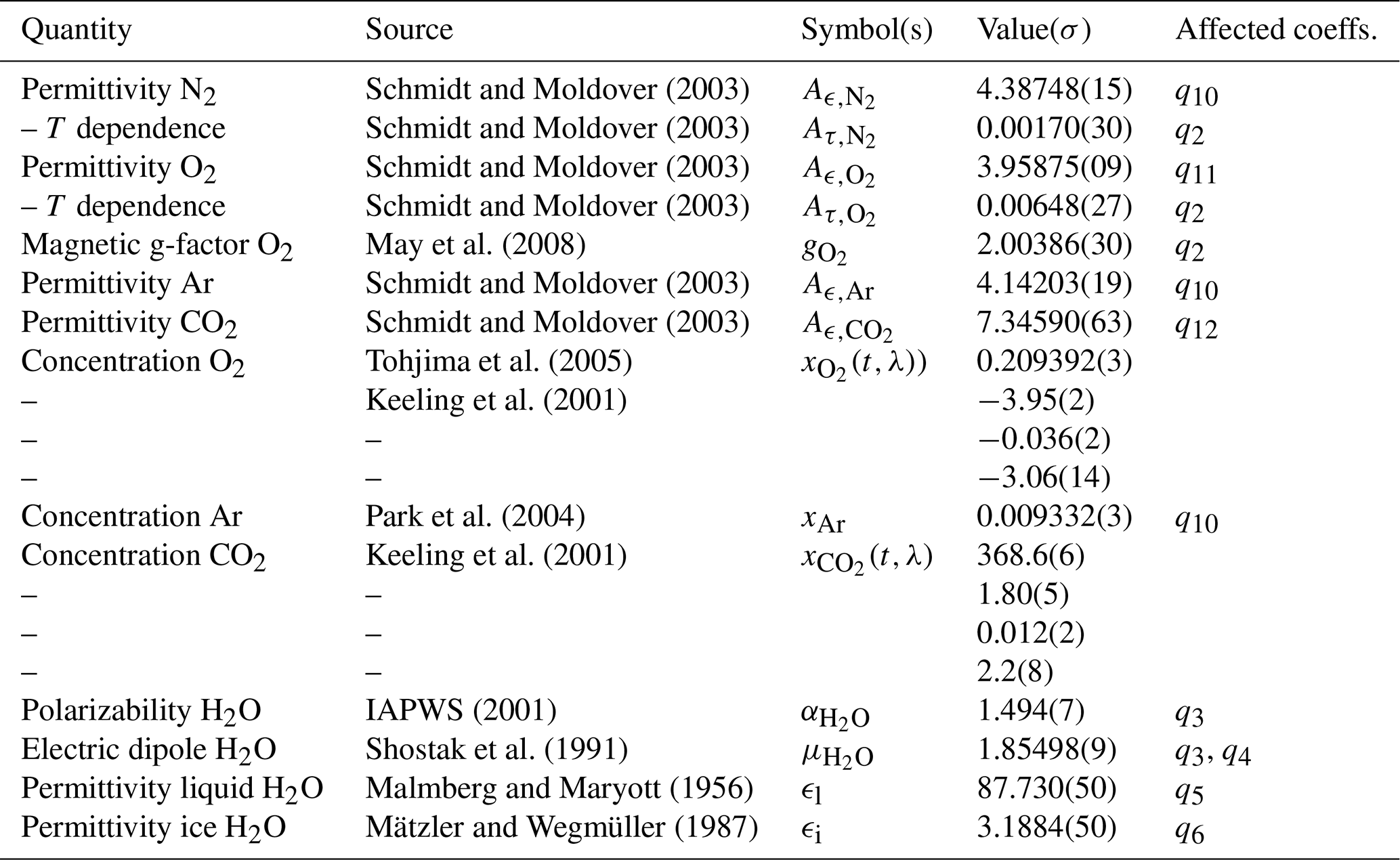
Because of the chosen ansatz for the macroscopic expression, most of the derivatives are negligible, and most experimental inputs influence only a single coefficient. The input parameters whose uncertainties can produce significant changes in the fitted q_i are collected in Table 2.

Schmidt and Moldover (2003)Schmidt and Moldover (2003)Schmidt and Moldover (2003)Schmidt and Moldover (2003)May et al. (2008)Schmidt and Moldover (2003)Schmidt and Moldover (2003)Tohjima et al. (2005)Keeling et al. (2001)Park et al. (2004)Keeling et al. (2001)IAPWS (2001)Shostak et al. (1991)Malmberg and Maryott (1956)Mätzler and Wegmüller (1987)

Table 2 Collected list of input quantities that have a sizeable impact in the final user expression

3.5 Error budget

Table 2 collects the list of primary inputs entering the microphysical model, and correspond to quantities that are either mdirectly measurable in laboratory conditions or determined through dedicated measurement campaigns. In total, the list contains 19 real-valued primary inputs.

The user expressions (28)–(38) contain a number of coefficients obtained by fitting to the microphysical model constructed upon those primary inputs. Consequently, each user-level coefficient inherits the dependence on the numerical values, and uncertainties of the primary inputs from which the microphysical model is built.

The user expression contains 18 coefficients, grouped as follows:

• 4 coefficients to describe the reference gas phase –namely refractivity of dry air and water vapour, and associated temperature dependences– following the structure of Aparicio and Laroche (2011).

• 2 coefficients describing the refractivity sensitivity dependence to atmospheric composition, specifically linked to variations in CO₂ and O₂.

• 4 coefficients related to average molar masses, three for the dry-air fraction (allowing variable CO₂ and O₂ composition), and one for water vapour.

• 8 coefficients describing contributions of hydrometeors – four for each condensed phase (liquid and solid) – including their dependence on hydrometeor shape under vertical and horizontal field polarizations.

In principle, propagating the dependence of these fitted coefficients on the 19 primary inputs would require the full matrix of partial derivatives, of dimension (18×19). However, the structure of the ansatz was chosen explicitly to minimize cross-dependencies between primary inputs and fitted parameters. As a result, most primary measurements influence only a single coefficient, and their impact on the remaining is either very small or entirely negligible.

The practical traceability table is therefore far simpler than the full derivative matrix. The primary inputs that significantly affect each fitted coefficient are identified in the last column of Table 2. The reduced set of non-negligible dependencies is presented in Tables 3 and 4.

Table 3 List of significant dependencies of the dry user coefficients q₁ and q₂, with respect to primary inputs. User coefficients are in SI units (N-units ⋅ kg⁻¹ m³). Units of the inputs and derivatives, follow the source units from their respective references, and are diverse: A_ϵ and A_τ in cm³ mol, molecular mass in amu, $g_{{\mathrm{O}}_{\mathrm{2}}}$ adimensional, polarizability α in 10⁻²⁴ cm³, electric dipole in Debye units. Uncertainty statistics σ are those that propagate to the coefficients, arising from the estimated uncertainties of the inputs.

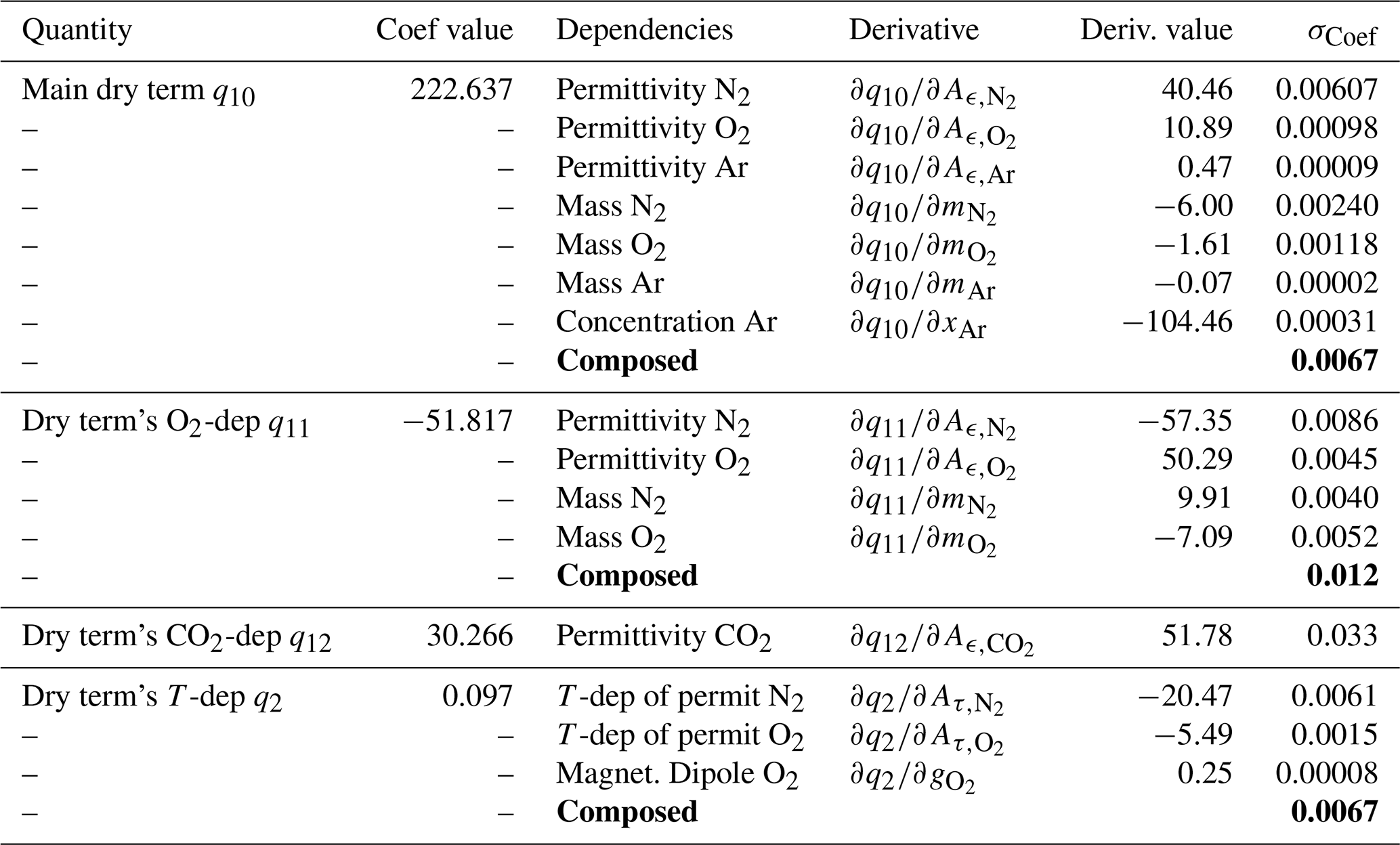
Table 4 As Table 3, for moist user coefficients q₃ and q₄, precipitated terms q₅ and q₆, and main molar mass coefficients m_d0 and m_w.

4 Discussion and analysis

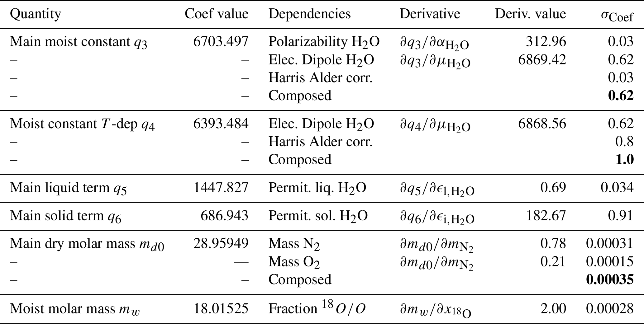
The microphysical model and the corresponding fitted user expression have been evaluated using best estimates of the primary laboratory or field-measured parameters listed in Table 2. These quantities carry uncertainties, that propagate into the user-level coefficients. This propagation serves two purposes: (i) assigning a total uncertainty to each fitted parameter, and (ii) identifying the dominant experimental sources of these uncertainties. The detailed propagation is summarized in Tables 3 (dry-air terms) and 4 (all other terms). As customary, uncertainties are expressed as std errors affecting the last digits. We discuss the fitted coefficients in turn:

• Main dry parameter q₁₀: The uncertainty is dominated by the dielectric response of N₂. The next most relevant contribution originates from the molar mass of N₂ (via the ${}^{\mathrm{15}}\mathrm{N}{/}^{\mathrm{14}}\mathrm{N}$ ratio), owing to the explicit dependence of the ansatz on density. The dielectric response of O₂, assuming the quoted uncertainty is reliable, contributes very little, whereas the mass uncertainty of O₂ (through the ${}^{\mathrm{18}}\mathrm{O}{/}^{\mathrm{16}}\mathrm{O}$ ratio) contributes more strongly than its dielectric term. The resulting coefficient, q₁₀=222.637(7), is sufficiently accurate for the intended applications (fractional uncertainty $\mathrm{3}\times {\mathrm{10}}^{-\mathrm{5}}$). Improved dielectric measurements of N₂ could modestly reduce the uncertainty (down to $\mathrm{1.3}\times {\mathrm{10}}^{-\mathrm{5}}$), though at that level limitations of the ansatz (e.g. missing nonlinearities) would likely dominate. This term contributes most to the refractivity.

• O₂ dry parameter q₁₁: For O₂, which is close in mass and polarizability to the mean air molecule, the uncertainty is shared among the dielectric responses and molar masses of both N₂ and O₂. The fitted value $q_{\mathrm{11}}=-\mathrm{51.817}\left(\mathrm{12}\right)$ is sufficiently accurate given the relatively small overall contribution of this term.

• CO₂ dry parameter q₁₂: The uncertainty is governed by the polarizability and mass of the CO₂ molecule. The coefficient q₁₂=30.266(33) has adequate accuracy, as its contribution to refractivity is small.

• Temperature-dependent dry term q₂: This coefficient is small and would vanish for an ideal gas of nonpolar molecules. It arises from temperature-dependent polarizability (intermolecular interactions), and the magnetic susceptibility of O₂. The latter is known very precisely, hence the quoted uncertainty is dominated by the temperature-dependent polarizability of N₂, attributed by Schmidt and Moldover (2003) to anharmonic vibrational effects. The coefficient q₂=0.097(6) is sufficiently accurate given its modest contribution.

• Main moist term q₃: The term includes contributions from the electric polarizability and permanent dipole moment of water, toguether with a dependence on molar mass. The uncertainty is dominated by the dipole moment of water, even though its measured value (Table 2) is already precise. The coefficient is q₃=6703.5(6), and this term is the second largest contributor to refractivity, though only in moist conditions.

• Temperature-dependent moist term q₄: The uncertainty is again dominated by the electric dipole moment of water, but mostly through the correlation factor g. The dipole is enhanced by molecular interactions described by a Buckingham factor and, critically, by a density and temperature-dependent correlation factor g(ρ,T) which is very specific to the interaction of water with other near molecules. Water forms transient aggregates such as dimers (Scribano et al., 2006), which increase the effective dipole moment beyond the single-molecule value. While the high-density behaviour of g is well constrained (Fernández et al., 1997), the low-density regime relevant here relies on the approximation $g(\mathit{\rho },T)\approx \mathrm{1}+h\left(T\right){\mathit{\rho }}_{\mathrm{w}}$, which carries significant uncertainty, and dominates the error estimate. The resulting coefficient is q₄=6393.5(10). Although moderately important in moist conditions, the current uncertainty is acceptable.

• Liquid water term q₅: Somewhat surprisingly, this term depends only weakly on the permittivity of liquid water ϵ_r≈90. With this strong response, water screens itself from the test field, so the uncertainty of ϵ_r has a modest effect. Most of the remaining uncertainty is aliased from correlations with water vapour in the fitting dataset. The fitted value q₅=1447.83(13) is satisfactory given the typically small amounts of liquid water.

• Solid water term q₆: Ice and snow have much lower permittivity ϵ_r≈3 and therefore exhibit weaker self-screening. The refractivity contribution is thus more sensitive to the dielectric uncertainty, which dominates the error budget of this term. The coefficient q₆=686.94(91) remains adequate given the small contribution of frozen water to refractivity.

A key point is that the dominant uncertainty in the main dry term, q₁₀ derives from the physical properties of the nitrogen molecule. This uncertainty is effectively constant in time to a precision much better than the quoted error. As discussed in Sect. 3.2, the dry-air term exhibits a slow temporal drift due to evolving atmospheric composition. However, this drift does not involve N₂, thus we can conclude that q₁₀ is constant to high accuracy.

The user model also includes several parameters describing the asphericity of hydrometeors. The model assumes uniform asphericity and a single canting angle, which are not expected to hold with high accuracy. Realistic hydrometeor populations involve heterogeneous and poorly known shape and orientation distributions, far more complex than an ensemble of aligned rotational ellipsoids. Consequently, SI-traceability cannot be guaranteed when aspherical hydrometeors contribute appreciably. For this reason, the propagation of the microphysical error has not been carried to the functions f_l(a_l;p) and f_i(a_i;p), nor to the eight parameters that govern them. Their purpose is not to yield precise refractivities for hydrometeors of known shape, but rather to bound the plausible range of refractivities when shapes and orientations are inherently uncertain, and to estimate the order of magnitude of hydrometeor-related effects such as polarization-dependent differential delay or the splitting of propagation paths.

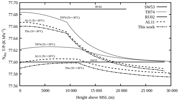
We may compare the current proposed formulation with several others in the literature. To illustrate the basic behaviour of dry-air refractivity, it is useful (Aparicio and Laroche, 2011) to examine $N\cdot T/P$, which is very close to 77.6 N-units K hPa⁻¹, and for some formulations exactly constant and denoted k₁. This comparison is shown in Fig. 3. Representative atmospheric states reveal a temperature and density dependence: at lower density (lower pressure, higher altitude), the asymptotic value of k₁ decreases; at lower altitude, and particularly in colder conditions, k₁ increases. Since GNSSRO impact in NWP peaks at around 200–300 hPa (approximately 8–10 km of altitude), the mean effective k₁ is likely closer to its lower-density value.

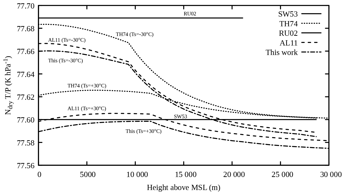
Figure 3 Quantity $N_{\mathrm{dry}}\cdot T/P$ evaluated with various available formulations, and including the present one. For realistic examples, the atmospheric states follow the lapse rates of a US Standard atmosphere profile, illustrating typical behavior at different altitudes and latitudes. Warm and cold examples are shown, with surface temperatures of $T_{\mathrm{s}}=-\mathrm{30}$ °C, and $T_{\mathrm{s}}=+\mathrm{30}$ °C. The compared expressions are (Smith and Weintraub, 1953, SW53), (Thayer, 1974, TH74), (Rüeger, 2002, RU02), (Aparicio and Laroche, 2011, AL11), and the present work. The current formulation depends on the composition; for consistency with the ROMEX experiment, 2022 values have been adopted.

This work also confirms a refractivity generally in the lower band within the literature formulations, except in colder denser conditions, where suggests results in the upper band. In general, these results suggest that the formulation by Rüeger (2002) appears to be too high by between 0.05 %–0.1 %, which agrees with the appearence of NWP bias if this formulation is used Aparicio et al. (2009); Healy (2011). The formulation (Thayer, 1974) reproduces significantly the qualitative dry-air behaviour indicated in Aparicio and Laroche (2011) and here, although also appears systematically high. The excess, though, is smaller, about 0.03 % in dry-air refractivity. However, although the dry-air behaviour of Thayer (1974) is good, it does not clarify how moist refractivity should be calculated, given the strongly nonideal behaviour of water vapor, which renders the expression ambiguous (Aparicio and Laroche, 2011). The formulation in Smith and Weintraub (1953) does not reproduce the temperature or density dependence, but appears to be an average compromise except at the densest conditions (cold conditions in the low troposphere). Finally, compared to AL11, the ensemble of modifications proposed here reduces slightly the average refractivity, by about 0.01 %, but maintains most of the density and temperature dependence.

In Fig. 3 it is also interesting to note that, whereas TH74 converges to a constant with altitude (its compressibility factor Z converging to 1), both AL11 and this work continue to show some descent. The compressibility factor in these latter also converges to 1, but these expressions contain some small but non-zero temperature dependence of $NT/P$, stemming from the magnetic dipole of the O₂ molecule, and expressed as term q₂ in the proposed expression. Figure 3 also indicates that, although (Rüeger, 2002) overestimates dry refractivity, it is better at low altitude. In retrospect, this is consistent with the primary application of that paper, which was for electronic distance measurements at surface level. Similarly, (Smith and Weintraub, 1953) underestimates refractivity in most of the troposphere, yet is better in the upper troposphere and low stratosphere, leading to a good average behaviour for GNSSRO.

Within ECCC, neither AL11 nor this formulation introduce a concerning bias. Upon significant increase of the GNSSRO volume, as for instance ROMEX data, thermodynamic indicators such as the bias profiles of temperature or geopotential against radiosondes are not dragged by more than 1 part in 10 000, consistent with the estimation of absolute accuracy of 0.01 %. However, initial GNSSRO use at ECCC (e.g. Aparicio and Deblonde, 2008), while positive, did drag thermodynamic profiles at the level of 0.1 %. Since GNSSRO bias is not only a function of the refractivity, it will be summarily mentioned that at ECCC, assimilation of GNSSRO also

1. uses GNSSRO data in the form of refractivity profiles

2. accounts for the deviation of air from ideal gas (Picard et al., 2008), both in the refractivity/pressure relationship, and in the hypsometric relationship

3. follows the horizontal drift of the tangent point over a profile (Bani-Shahabadi et al., 2018, 2020)

4. the hypsometric equation considers the variability of the strength of gravity with latitude and altitude, and through a wind-dependent vertical component of the Coriolis force (Eötvös, 1919)

all of which have some impact in the GNSSRO observation minus background statistics.

Of all these elements, and concerning the refractivity expression and the bias between GNSSRO and an NWP system, the dry component (here, q₁ with its subcomponents, and q2) is the most important, as it detemines the behaviour in the core region of GNSSRO, between 300 and 50 hPa, where these data are more accurate and have higher impact). Among the other elements besides refractivity, the non-ideal gas effects are judged as next in importance, with the Coriolis force being small but systematic, thus affecting bias.

5 Conclusions

A previous study has been revisited, with particular attention to re-evaluating the error budget and to identifying the main limitations to improved accuracy. Beyond several minor refinements, the atmospheric composition is identified as one of the elements that constrain accuracy within the desired performance range. In view of the secular evolution of O₂ and CO₂ abundances, their fractions are made explicit independent variables.

$$\begin{array}{}\text{(47)}& {\displaystyle }N=\left[q_{\mathrm{1}}+\mathrm{0.097}\left(\mathrm{6}\right)\cdot \mathit{\tau }\right]{\mathit{\rho }}_{\mathrm{d}}+\text{(48)}& {\displaystyle }\left[\mathrm{6703.5}\left(\mathrm{6}\right)+\mathrm{6393.5}\left(\mathrm{10}\right)\cdot \mathit{\tau }\right]{\mathit{\rho }}_{\mathrm{w}}+\text{(49)}& {\displaystyle }\mathrm{1447.83}\left(\mathrm{13}\right)\cdot f_{\mathrm{l}}(a_{\mathrm{l}};p)\cdot {\mathit{\rho }}_{\mathrm{l}}+\text{(50)}& {\displaystyle }\mathrm{686.94}\left(\mathrm{91}\right)\cdot f_i(a_i;p)\cdot {\mathit{\rho }}_i\end{array}$$

where q₁ may be expressed as a function of O₂ and CO₂, if these are available:

$$\begin{array}{}\text{(51)}& \begin{array}{rl}{q}_{\mathrm{1}}(x_{{\mathrm{O}}_{\mathrm{2}}},x_{{\mathrm{CO}}_{\mathrm{2}}})& =\mathrm{222.637}\left(\mathrm{7}\right)-\mathrm{51.817}\left(\mathrm{12}\right)\\ & \cdot \left(x_{{\mathrm{O}}_{\mathrm{2}}}-\mathrm{0.2095}\right)+\mathrm{30.266}\left(\mathrm{33}\right)\cdot x_{{\mathrm{CO}}_{\mathrm{2}}}\end{array}\end{array}$$

In all cases, the parentheses express the uncertainty in the coefficients as stemming from the uncertainty in the experimental sources collected in the microphysical model.

Alternatively, using fits to recent decades of measured atmospheric composition, the expression for q₁ may be written instead as a function of time. Such a fit to the composition is suggested in Eqs. (15) and (16) and will be valid as long as it continues to represent the main trend of the observed evolution, presumably at least several decades. The time-dependent q₁ may then be expressed as:

$$\begin{array}{}\text{(52)}& q_{\mathrm{1}}\left(y\right)=\mathrm{222.654}\left(\mathrm{7}\right)+\mathrm{0.000259}\cdot y_{\mathrm{2000}}+\mathrm{2.24}\times {\mathrm{10}}^{-\mathrm{6}}\cdot y_{\mathrm{2000}}^{\mathrm{2}}\end{array}$$

with y₂₀₀₀ time in years since 2000. This is the only coefficient in Eq. (47) that shows a significant dependence on composition. At Environment and Climate Change Canada, Eqs. (47) and (52) have been implemented operationally as an update to AL11, which was in use since 2011. For practical operational use, it was selected to use the time-dependent form of q₁, which implicitly describe composition. As noted above, the uncertainty associated with seasonal and latitudinal variability in composition is not dominant relative to the uncertainty in absolute concentrations. Under these circumstances, the expression q₁(y), which has been simplified, is not inferior to a more complex $q_{\mathrm{1}}(x_{{\mathrm{O}}_{\mathrm{2}}},x_{{\mathrm{CO}}_{\mathrm{2}}})$.

The refractivity expression exhibits a small dependence on the polarization state when hydrometeors (rain, snow, or ice) are non-spherical. This dependence is captured through the shape factors f_l(a_l;p) and f_i(a_i;p). The approximate magnitude of their impact has been evaluated: it is modest, but is measurable as differential path delay, and should also be measurable as a form of double refraction for rays traversing extended regions of dense precipitation during an occultation. Measuring this effect requires a dual-polarization receiver. Such receivers, sensitive to both linear polarizations independently, have been launched in recent years.

For many applications of the refractivity expression – such as its routine use in the assimilation of refractivity in Numerical Weather Predicition –, this update introduces only small differences, and the changes with respect to Aparicio and Laroche (2011) are minor. As observed at other operational centers, ECCC identified that the absence of bias between GNSSRO and model fields becomes particularly critical at higher observational volumes. This motivated the implementation of the present update, even though AL11 had remained generally adequate.

The comparison between the different existing formulations suggests that the threshold of 0.1 % uncertainty (that is, fractional uncertainty of 10⁻³) is exceeded, provided a non-ideal gas formulation is adopted. The difference between existing formulations, with some differences between the implementation details, in the assumptions about the nature of atmospheric air, and the link to fundamental measurements, indicates rather a difference of 0.01 % (thus 10⁻⁴) between studies, provided they account for non-ideal gas effects. Finally, the formal uncertainty as propagated in this study from fundamental measurements indicates a fractional dry-air uncertainty of about $\mathrm{3}\times {\mathrm{10}}^{-\mathrm{5}}$ of dielectric origin, thus if the variabilities in composition are accounted.

This study suggests that, whereas a confirmation of the low dielectric uncertainty would be welcome, the remaining sources of refractive uncertainty are, first, of thermodynamic origin, in the non-ideal gas behaviour of air, and particularly water vapour, and second, in details of composition, from the evolution of CO₂ and O₂ to uncertainty in the molar mass, by uneven isotopic composition, where notably water vapour and N₂ should be mentioned. These diverse residual sources of uncertainty – of the order of 10⁻⁵ –, limit our knowledge of refractivity to not be better than 10⁻⁴ in fractional uncertainty unless a model of considerably more complex nature was prepared. However, these residual sources of uncertainty do not prevent reaching that stated level of 10⁻⁴, or 0.01 %, which we judge as sufficient for NWP purposes. Concerning hydrometeors, the model does maintain this stated accuracy even under the highest densities of hydrometeors that are likely in the atmosphere, for a given amount of liquid water, ice, their shape and orientation. It is however unlikely that the atmosphere contains amounts of water, ice, shapes and orientations that are sufficiently uniform for this to be meaningful in practice. The natural heterogeneity of hydrometeors introduces an uncertainty in the use of an electromagnetic model, above the physical uncertainty of that model. In the atmosphere, that may amount to perhaps as much as 50 % of the hydrometeor contribution to refractivity. However, the hydrometeor contribution is generally less than 1 % of the total refractivity, and in the upper atmosphere much less. Therefore this heterogeneity may dominate uncertainty only when the hydrometeor contribution is large, which is not the case in most of the upper atmosphere, and may happen only at hydrometeor densities above 0.02 (grams of hydrometeor per kg of air). It is thus recommended to allow for a hydrometeor-dependent uncertainty estimate, composed of the mentioned 10⁻⁴ fractional uncertainty of the electromagnetic model, plus a fraction of the estimated hydrometeor contribution, derived not from electromagnetic uncertainty but from their large variability.

Several other applications may benefit from the expressions presented here. These include:

1. Radio-optical measurements, such as GNSSRO, in decadal climate studies, where cumulative changes in atmospheric composition produce a non-negligible drift.

2. Situations where traceability between radio-optical and thermodynamic measurements is essential, since traceability requires a quantified uncertainty chain.

3. Investigations of the polarization dependence introduced by hydrometeors.

4. Estimation of atmospheric delay, such as GNSS zenith total delay (ZTD), or subtraction of this delay, such as radar altimeters