Measured methane emissions from a metropolitan wastewater treatment lagoon in Victoria Australia are substantially higher than report emissions based on emission factors

Wastewater treatment facilities contribute ∼ 8 % of global anthropogenic methane (CH₄) emissions. Accurate measurements of CH₄ emissions not only improve greenhouse gas (GHG) emission estimates from the facilities but also expand our understanding of operational impact on emissions, thus enabling the development of effective mitigation strategies. In this study, CH₄ emissions were measured during summer and winter seasons at an aerobic lagoon at a large sewage treatment plant in Australia. Line-averaged CH₄ concentrations were measured by open-path lasers and CH₄ fluxes were calculated using inverse-dispersion modelling. Methane fluxes showed temporal and spatial variations over the measurement periods, and correlated with wastewater dissolved methane, flow rate, and aerator operation. The annual GHG emission of 80 308 t CO₂-e yr⁻¹ represents ∼ 25 % of CH₄ production captured by the anaerobic digestion pot and is approximately 2.0–2.3 times higher than the National Greenhouse and Energy Reporting Scheme (NGERS) reported emissions of the aerobic lagoon.

1 Introduction

Wastewater treatment plants (WWTPs) are a significant source of greenhouse gas (GHG) emissions resulting from the environments that have high supply of organic matter and nutrients (Czepiel et al., 1993; Daelman et al., 2012). Substantial methane (CH₄) emissions from wastewater treatment facilities have been reported, with this sector contributing to ∼ 5 %–8 % of global anthropogenic CH₄ emissions (Ye et al., 2022), following livestock (32 %), oil and gas (25 %), landfill (13 %), and coal mine (11 %). Methane contributes to climate change: its global warming potential is 27 times that of carbon dioxide (CO₂) in a 100-year time span and 80 times CO₂ considering a 20-year timeframe, according to the IPCC (2021) report. To achieve the goal of the Paris Agreement (e.g., limiting global temperature rise to well below 2 °C above pre-industrial levels), reducing WWTP's GHG emissions is an important climate action to help to prevent the worst impacts of climate change. Furthermore, assessing the environmental impacts of GHGs, has become a necessity for the long-term sustainability of WWTPs (Mohsenpour et al., 2021). To reduce GHG emissions from WWTPs and achieve the Australia Water sector's goal of net zero emissions by 2035, it requires a better understanding of current GHG emission rates from facilities, as well as an evaluation of the main drivers of emissions, to implement appropriate mitigation measures. Currently there are large uncertainties in estimating these emissions, as WWTPs use generalised, default emission factors (National Greenhouse and Energy Reporting Scheme (NGERS), Method 2) (Bartram et al., 2019; NGER, 2022), which may not accurately represent local conditions and the specific management practices.

Across various nations, anaerobic ponds are commonly used as the first step in municipal sewage treatment. Raw sewage enters anaerobic ponds and settles into different layers, with a liquid layer over the sludge to prevent oxygen from reaching it during microbial digestion. Anaerobic microbes present in the sludge digest the organic matter (OM) in influent raw sewage and settle to the bottom of the pond along with organic and inorganic solids. Sludge can be removed and reused for land application. Aerobic ponds are used following the anaerobic ponds where aerators are deployed to introduce air into the water column. This allows for aerobic respiration to occur, where oxygen and other microbes in the wastewater are mechanically churned, helping to break down OM. The bacterial-containing chunks settle to the bottom of the pond. During these processes, CH₄, nitrous oxide (N₂O), and ammonia (NH₃) emissions are emitted into the atmosphere.

This study focussed on measuring CH₄ emissions at a large lagoon-based sewage treatment facility in Victoria, Australia. It occupies a site of more than 10 000 ha, serving up to 2.5–3 million residents. The area of focus for this emissions measurement research is known as 25W Pond 1, which is adjacent to a covered anaerobic digestion pot, where the raw sewage influent undergoes preliminary treatment. The majority of the treated wastewater after the anaerobic pot enters directly into the Pond 1 (25W) for aerobic treatment with surface aerators, the rest of the treated wastewater is pumped into an anoxic-aerobic activated sludge plant for secondary treatment. The sludge generated from the activated sludge plant is returned to the Pond 1 for treatment. The 25W Pond 1 system has 53 surface aerators distributed across the pond (the layout of aerators is shown in the Supplement), and the aerators operational time is often controlled by the flow rate, for example, when the flow rate is higher in the morning, aerators run for longer or more aerators are switched on. Furthermore, the aerators (when on) increase the oxygen content in their immediate vicinity, while the water region far from the aerators has less or no oxygen (Nguyen et al., 2024). This operating regime contributes to the spatial and temporal variation of the conditions within the pond (Li et al., 2024; Liu et al., 2023), which makes it very challenging to accurately measure GHG emissions (Delre et al., 2017).

Different measurement technologies have been reported for measuring GHG emissions in the WWTPs either for integration emission quantification or identification of specific facilities (He et al., 2025). In many jurisdictions the chamber technique is a regulatory standard for direct gas emission measurements (Ye et al., 2022; Morales-Rico et al., 2024; Parravicini et al., 2022). However, chamber measurements are susceptible to the disturbances that result from isolating the source inside a chamber (e.g. it is challenging to measure the emissions from surface aerators; Morales-Rico et al., 2024). The small measurement footprint of chambers (covering less than 1 m² of surface) is likely to be a tiny fraction of the source area. Chambers are also poorly suited for long-term measurements due to the labour cost.

World-wide efforts are underway to implement measurement methodologies that are more accurate than chambers (and cheaper and logistically simpler to use) (Reinelt et al., 2017; Yver Kwok et al., 2015; Jensen et al., 2017; Delre et al., 2017; Samuelsson et al., 2018). One such alternative is the inverse-dispersion modelling (IDM) approach (Flesch et al., 2011; Bühler et al., 2022), which is the basis of this study. This technique follows the simple idea that an emission source increases the downwind gas concentration, and that a measurement of downwind concentration (above the upwind background level) can be used to quantify the emission rate from the source area. The correlation between the emission rate and concentration is calculated with an atmospheric dispersion model (Flesch et al., 1995). IDM is a non-interference/non-intrusive technique that does not alter the measurement environment. It has modest measurement requirements and is well suited for long-term deployment. We recently reported our studies of measuring CH₄, N₂O, and NH₃ emissions from a sludge drying pan at a WWTP using IDM methods coupled with open-path spectroscopic techniques (Bai et al., 2023, 2025).

The objectives of this study are to measure CH₄ emissions from the 25W Pond 1 using IDM coupled with open-path laser techniques, explore the main drivers of emissions from the facility, and validate the NGERS estimate.

2 Materials and Methods

2.1 Experimental site

This study was conducted at a sewage treatment plant, located in Victoria, Australia. One of two identical treatment lagoons with surface aerators, 25W Pond 1 was chosen for this study. Wastewater after being treated from the anaerobic Pot flows directly into 25W Pond 1, and travels through the pond in an east-west direction. Other research using hoods and mobile survey techniques have shown that the Pond 1 have the highest CH₄ emissions at the sewage treatment plant and therefore are the largest concern with respect to the CH₄ emissions. This is because it is the first pond after the covered anaerobic pot where anaerobic digestion of raw sewage takes place. Biogas is generated underneath the cover and is collected and sent to onsite power generation facilities for energy generation. Effluent from the anaerobic pot is saturated with dissolved methane, once agitated and/or under different atmospheric pressure (in Pond 1), releases CH₄ emissions to the environment. Wastewater in the downstream facultative ponds such as Pond 2 has a much lower chemical oxygen demand (COD) than in Pond 1, and Pond 2 typically emits less than $\mathrm{1}/\mathrm{10}$ of the CH₄ emissions compared to Pond 1. The 25W Pond 1 has dimension of 250 × 1010 × 3 m (width × length × depth) (Fig. 1). There are also several lagoons located on the south of the Pond 1, while to the north of Pond 1 the terrain is flat, covered with short grass, and there are no tree lines or tall buildings nearby. Further north, there is a corn field, about a few hundred meters north of the pond. A sludge drying pan area is located ∼ 200 m to the west of the pond. This layout allows for CH₄ measurements when there are winds tending from the north, because to the north within a radius of a couple of hundred meters, there are no other CH₄ sources interfering with the measurements. The average minimum/maximum ambient temperature was approximately 18 and 26 °C for summer, 12 and 19 °C for winter, respectively. A total of 1.4 and 37.4 mm of precipitation was observed over the summer and winter measurement period, respectively.

Figure 1 The layout of experimental site with one upwind open-path laser (light blue line with triangles), and two downwind open-path lasers (green and purple for summer campaign, green and blue for winter campaign). The Red triangle shows the weather station location during the summer campaign, while the dark blue triangle shows the weather station location during the winter campaign (Source: Imagery © 2024 Airbus, Map data © Google Earth).

2.2 CH₄ concentrations measured with open-path laser sensors

Three open-path lasers (OPL) were deployed in each campaign measuring line-average CH₄ concentration (in ppm-m). Two of the three laser sensors used in this study were from Unisearch Associates Inc. Canada (LasIRView, OPL_C33, OPL_C34), the third laser was from Boreal Laser Inc. Canada (Gasfinder 2.0, OPL_C1013). The concentration sensor sends a collimated beam from a tunable infrared laser diode to a retro reflector, from which the beam is reflected back to the receiver optics and a detector. The outgoing beam is absorbed by CH₄ molecules over the measurement path (between the laser and retro reflector), giving a measure of CH₄ concentration. Line-averaged CH₄ concentration is obtained every few seconds. The precision of CH₄ concentration at a 100 m path length is: < 1 ppb for the Unisearch laser, 20 ppb for the Boreal laser.

To avoid surrounding ponds contributing to the emission of target source Pond 1, our experimental layout was designed for only northerly winds, and data collected with other wind directions was not counted for the flux calculation. More details are shown in below filtering criteria section. In each campaign, two lasers were set up at the south of the pond to measure the downwind concentrations and one laser at the north of the pond to measure the upwind concentrations so that the enhance concentrations from the Pond 1 can be determined. Each instrument was deliberately matched to the expected CH₄ concentration range at its location. The higher-precision Unisearch laser was used in the western low-emission zone and the Boreal laser in the eastern high-emission zone: OPL_C33 was located the western side of the pond (west laser) and OPL_C1013 was located the eastern side (east laser), close to the anaerobic Pot cover area. The third laser OPL_C34 (background laser) was located at the north of the pond measuring the upwind concentration. Noted the upwind laser remained at the same location during the two measurement periods as the land cover was similar and the background condition remained stable during the measurements (Fig. 1).

Each laser and retro reflector were mounted on a separate tripod at approximate 1.50 m above the ground, with the pathlength of 100–150 m between the laser and retro reflector. Each OPL was powered by a 12 V battery coupled with solar panels. Prior to the measurements, three lasers were conducted cross-calibration on site for at least 48 h to examine their stability and performance under same climate conditions. Gas emission measurements were begun from 8 February to 12 March 2024 for the summer campaign, and from 15 August to 5 October 2024 for the winter campaign. Measurements from both campaigns are included in this paper.

2.3 Pond 1 wastewater samples collected using drone

To examine the Pond 1 effluent chemical and physical property and understand how these factors are associated with the flux measurements, wastewater samples were collected in September using a drone along the middle of the pond at 5, 50, 100, 150, 200, 275, 350 and 500 m from the Pot covered area (sampling locations are shown in Fig. S1 in the Supplement). For each sample, the temperature, redox, pH, and dissolved oxygen were analysed immediately on site. Subsamples (850 mL each) were also taken at each location and analysed in the laboratory for other properties analysis.

2.4 CH₄ flux calculations using IDM technique

The IDM technique is a classic micrometeorological method that calculates emissions from gas measurements taken in the free air. The micrometeorological methods are generally preferable to other approaches, as they are non-intrusive techniques that are suitable for long-term measurements. Consider a treatment pond that is emitting gas to the atmosphere at an unknown rate Q, which causes the average gas concentration (C) downwind of the pond to rise above the background value (C_b). In the IDM technique, the measurement (C−C_b) is used to determine Q with the aid of an atmospheric dispersion model (Windtrax). WindTrax is a software (http://www.thunderbeachscientific.com, last access: 12 December 2025) based on the backward Lagrangian stochastic dispersion model (bLs) for calculating gas emission rate from a source area (Flesch et al., 1995). WindTrax uses the bLs method, which is based on Monin-Obukhov Similarity Theory, and simulates the relationship between concentration (C−C_b) and emission rate Q, ($C/Q$)_sim. Because the Q vs. (C−C_b) relationship depends on wind conditions, one must also make wind measurements.

In this study, open-path CH₄ sensors were located to the south and north of the experimental pond. During northerly winds, this configuration allowed upwind (C_upwind) and downwind (C_downwind) measurements from the experimental pond, but not the southern ponds. Following Flesch et al. (2004), the CH₄ flux Q_IDM is calculated using IDM method following the equation (Eq. 1):

$$\begin{array}{}\text{(1)}& Q_{\mathrm{IDM}}=(C_{\mathrm{downwind}}-C_{\mathrm{upwind}})/(C/Q{)}_{\mathrm{sim}}\end{array}$$

where Q_IDM is the CH₄ gas emission rate (µg m⁻² s⁻¹), and C_downwind, C_upwind is the line-average gas concentrations (in ppm) measured by downwind and upwind laser sensor, respectively (Fig. 1). The value of ($C/Q$)_sim is the simulated ratio of line-average concentration and emission rate, calculated by WindTrax modelling based on the ambient temperature and pressure, wind statistics, and atmospheric turbulent parameters.

A three-dimensional (3-D) sonic anemometer (CSAT-3, Campbell Scientific, Logan, Utah, USA) coupled with a datalogger (CR23X, Campbell Scientific, Logan, Utah, USA) was located at the south of the Pond 1 at a height of 2.34 m above the ground (Fig. 1), to record wind statistics at a frequency of 10 Hz that are needed for IDM calculation. 15 min statistics includes the friction velocity (u_∗, m s⁻¹), turbulent velocity (u, v, w, T), and its variance (u², v², w², T²) and covariance (uT, uv, uw, vT, vw, wT) in three dimensions, as well as ambient temperature (°C), wind speed (m s⁻¹), and wind direction. Ambient pressure (mbar) and rainfall (mm) were obtained from Bureau of Meteorology.

The concentrations of CH₄ were averaged into 15 min intervals then merged with wind variables as inputs for the IDM flux calculation using SAS software (SAS 9.4, SAS Institute Inc. Cary, NC, USA). The atmospheric turbulent parameters including Obukhov stability length (L, m), surface roughness (z0, m), and turbulent velocity fluctuation ($\mathit{\sigma }u/u_{\ast }$, $\mathit{\sigma }v/u_{\ast }$, and $\mathit{\sigma }w/u_{\ast }$) were also calculated for the IDM simulation.

2.5 CH₄ flux calculation filtering criteria

Following Flesch et al. (2016), the data for CH₄ emission calculations using the IDM methods were not counted when:

1. atmospheric turbulent conditions were poor: u_∗ < 0.1 m s⁻¹, $\left|L\right|$ < 2 m, z0 > 0.05 m,

2. the laser light level returned by the retro reflector was < 6000 or > 12 000,

3. the relationship between the measured external and reference signal R² was < 96,

4. the difference in concentration between the upwind measurement and background level simulated by IDM (WindTrax model) was > 0.02 ppm,

5. the upwind laser concentration measurement was < 1.8 ppm,

6. the percentage of source area covered by the touchdowns was < 20 %,

7. wind direction was > 40 and < 330°.

2.6 Average Pond 1 CH₄ flux calculation

The influent in the eastern part of the pond is directly connected to the anaerobic pot, where dissolved methane is high. By contrast, the western part of the pond has lower dissolved methane. We expected this to create a gradient of emissions from the eastern to western part of the pond. Because of the size of the pond, a single laser was not sufficient to capture the full pond, and instead two lasers were used to measure emissions along the gradient. Formally, this is a type of stratified sampling that scales each laser's measurements (eastern pond area and western pond area) to the full-lagoon emissions. The classic way to do post-stratification when using stratified sampling is to weight the estimate by the area that each strata represents (i.e., take a weighted average). In the summer campaign, the pond was divided into two strata of similar sizes (∼ 50 %–50 %). The total average emission was thus (0.5 times flux1 + 0.5 times flux2) × total pond area. The weights were varied by ±5 % to test the sensitivity of the results to this assumption and to provide a range of emissions for the measurements. The total emission for the summer campaign thus ranged from a low estimate of (0.55 times flux1 + 0.45 times flux2) × total pond area to a high estimate of (0.45 times flux1 + 0.55 times flux2) × total pond area. In the winter campaign, the east laser was closer to the Pot end covered area. The pond was divided into two strata of varying sizes (∼ 70 % west–30 % east). The total average emission was thus (0.70 times flux1 + 0.30 times flux2) × total pond area. After propagating uncertainty in the weights (±5 %), the total emission for the winter campaign ranged from a low estimate of (0.75 times flux1 + 0.25 times flux2) × total pond area to a high estimate of (0.65 times flux1 + 0.35 times flux2) × total pond area.

2.7 CH₄ flux uncertainty

There are four sources of relative uncertainty in our flux estimate: instrument precision (e₁ = 2 %), inversion-dispersion model (e₂ = 20 %) (Laubach and Kelliher, 2005), sampling uncertainty (i.e., the standard error, SE, calculated using the number of observations and standard deviation among the 15 min measurements, which contributes around e₃ = 1.2 % to 4.0 %), and the pond area represented by each laser in our weighted average (e₄ = 2.0 % error in total flux for the summer campaign, and e₄ = 5.2 % for the winter campaign, coming from varying the weight by ±5 % around their centred value, see section 2.6, resulting in a range of total average emission). These four sources of uncertainty are added in quadrature (sqrt ($e_{\mathrm{1}}^{\wedge \mathrm{2}}+e_{\mathrm{2}}^{\wedge \mathrm{2}}+e_{\mathrm{3}}^{\wedge \mathrm{2}}+e_{\mathrm{4}}^{\wedge \mathrm{2}}$), where the e_i's are the different error terms) to propagate the uncertainty and get our final estimates. Note that the total uncertainty is dominated by the inverse-dispersion model term (e₂) as the terms are added in quadrature.

To convert from relative uncertainty to absolute uncertainty (1σ), the 1σ figure was calculated using the definition for the coefficient of variation (CV) to represent the relative uncertainty (CV = 1σ/mean). Solving for sigma gives: 1σ = CV × mean. For example, using a CV of 20.6 % and a mean flux of 386.5 µg m⁻² s⁻¹ for the averaged Pond 1 in this study, a 1σ value of 79.6 µg m⁻² s⁻¹ is obtained.

3 Results and Discussion

3.1 Spatial and temporal variations of CH₄ fluxes

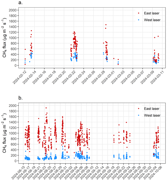
15 min CH₄ fluxes from Pond 1 varied spatially between the eastern and western pond areas (Fig. 2). Higher fluxes were observed at eastern pond area, ranged from ∼ 200 to over 1900 µg m⁻² s⁻¹, and lower fluxes ranged from ∼ 13 to over 570 µg m⁻² s⁻¹ were observed at western pond area. Furthermore, a clear 24 h diurnal pattern in the fluxes was observed at the eastern pond area, with lower emissions around midday and higher emissions at night-time or early morning. This diurnal pattern of maximum CH₄ emission at 08:00 am local time (LT) was also reported in Glaz et al. (2016). In contrast, no obvious diurnal pattern of the emissions was observed at the western measurement location.

Figure 2 15 min CH₄ fluxes from western (blue) and eastern area (red) of sewage treatment 25W Pond 1 measured over the summer season (a) from 12 February to 10 March 2024, and the winter season (b) from 15 August to 5 October 2024 in Victoria, Australia.

Daily averaged CH₄ fluxes varied among the seasons (Fig. 2). In the summer season, the daily average of CH₄ flux was 252.0 (±9.4, n = 139) (±SE for sampling uncertainty, n, observation numbers) and 582.1 (±23.3, n = 185) µg m⁻² s⁻¹ from the western and eastern pond area over the 5-week measurement period, respectively. In the winter season, the daily averaged CH₄ flux was 134.7 (±2.3, n = 797) and 874.2 (±10.6, n = 692) µg m⁻² s⁻¹ from western and eastern pond area over the 7-week measurement period, respectively. The emissions at eastern pond area were ∼ 2–6 times higher than that at western pond area, during both winter and summer measurements. The much higher eastern flux measurement in the winter campaign was mainly due to the laser measurement location being much closer to the anaerobic Pot covered area than during the summer measurement campaign. In contrast, the laser's locations at the western pond area remained the same during both summer and winter campaigns and the pond measurements were higher in summer than that in winter by 46 %.

The measured winter flux at western pond area was much higher than the higher range of the reports, e.g., the anerobic ponds in Australia (7 ± 1 g m⁻² d⁻¹) (Hernandez-Paniagua et al., 2014), duckweed treatment ponds of 1276 ± 299 mg CH₄ m⁻² d⁻¹ in the US (Sims et al., 2013), organic matter enriched sludge treatment wetlands of 1900 mg CH₄ m⁻² d⁻¹ in Norway (Søvik and Kløve, 2007), and 5400 mg CH₄ m⁻² d⁻¹ in Spain (Uggetti et al., 2012). Different measurement techniques, wastewater composition, climate conditions and operation management could introduce variability of methane fluxes (Reinelt et al., 2017).

3.2 Main drivers of CH₄ fluxes from 25W Pond 1

3.2.1 Wastewater chemical and physical properties and flow rate

The composition and load of the wastewater played important roles in the spatiotemporal dynamics of gas emissions (Glaz et al., 2016). The wastewater sampling collected along the middle section of Pond 1 in September showed that dissolved methane, biological oxygen demand (BOD), COD, and wastewater temperature decreased with distance from the Pot covered area (Fig. 3), in contrast, dissolved oxygen, pH, and redox positively correlated with distance from the anaerobic Pot covered area (P < 0.05). This decreasing trend of dissolved methane would explain the spatial variation of pond emissions and the difference in measured CH₄ fluxes between the eastern and the western part of the pond. Linear correlations with correlation coefficient (R) and P value are shown in Fig. 4.

Figure 3 Variations of dissolved methane, BOD, COD, SS, VSS, NH₃, TCN, VFA, pH, and dissolved oxygen shown with increasing distance from the cover area. Wastewater samples were collected by drone along the middle part of Pond 1 between 10:00–12:30 LT on the 10 September 2024 at 5, 50, 100, 150, 200, 275, 350, and 500 m from the cover, and extra samples were also collected at the PotCod, the jetty area (marked with an “x”) and Pond 1 outlet (0, 500, and 1000 m from the cover, respectively) on the same day.

Figure 4 Correlations between wastewater sample contents including dissolved methane, BOD, COD, SS, VSS, N-NH₃, TCN, VFA, pH, and dissolved oxygen and the distance from the anaerobic cover. Samples were collected by drone along the middle part of Pond 1 between 10:00–12:30 LT on the 10 September 2024 at 5, 50, 100, 150, 200, 275, 350, 500 m from the anaerobic cover, extra samples were also collected at the PotCod and the jetty area (0 and 500 m from the cover) on the same day. Linear correlation coefficient (R) and P value are also shown.

Wastewater flow rates (Fig. 5) showed a 24 h diurnal trend through the pot-pond area: lower flow rates before midday and higher flow rates in the evening and early morning. The winter measurement as an example is shown in Fig. 5. A similar diurnal pattern has also been reported in the literature (Mannina et al., 2018; Bühler et al., 2022; Guisasola et al., 2008). This diurnal pattern of flow rates was similar to the CH₄ flux diurnal variation, but the latter showed a time lag of ∼ 1–2 h (Fig. 5, red dots and red line). This is not surprising as, together, Pond 1 and the Pot covered area are a large area, and it takes 1–2 h for the wastewater to flow into the area where the laser measures the footprints of emissions. Besides this, hourly mean fluxes from the eastern pond area were positively correlated to hourly mean wastewater flow rates (R = 0.49, P < 0.001). This relationship was also reported in Glaz et al. (2016). However, the mean flux from the western pond area did not show an obvious correlation to the flow rate. As stated previously, the emission variation was associated with wastewater dissolved methane concentrations. At the western end of the pond the concentration of dissolved methane was negligible and therefore, there were lower CH₄ fluxes.

Figure 5 24 h diurnal variation of average wastewater flow rate and CH₄ fluxes during a winter campaign at 25W Pond 1 from 15 August to 5 October 2024.

3.2.2 Aerators operation

The surface aerators closest to two downwind measurement lasers were examined, and the fluxes were compared for three conditions: before the surface aerators were all switched off, when they were off, and when they were switched on again. For the aerators close to the east laser, hourly fluxes were 830.2, 296.8, 1453.0 µg m⁻² s⁻¹ for the periods before these aerators were all switched off, when they were off and when they were switched on again, respectively, on 23 August, and 1139.8, 251.2, 766.0 µg m⁻² s⁻¹, for the same periods on 6 September 2024. In contrast, on the west end of the pond, hourly fluxes were 90.0, 81.0 and 130.0 µg m⁻² s⁻¹ on 23 August for the periods before, during and after the off event, respectively, and 191.0, 121.0 and 125.0 µg m⁻² s⁻¹ for the same periods on 6 September 2024, respectively. Therefore, the surface aerators off events at the eastern pond area substantially decreased the emissions flux by 80 %.

3.2.3 25W Pond 1 daily CH₄ flux and annual GHG emissions

The average daily CH₄ flux from 25W Pond 1 was 8.78 and 7.52 t d⁻¹ over the summer and winter measurement period, respectively, by taking the mean of both fluxes at eastern and western pond area and multiplying by the total pond area (∼ 244 000 m²) (Table 1). It was found that during the summer campaign, fluxes over the western pond area were nearly 2 times higher than that of the winter campaign (252 vs. 134 µg m⁻² s⁻¹). This is likely associated with the sludge dredging events at Pond 1 between June and July 2024 (only weeks before the start of winter campaign). The dredging took place at the location where the western laser was measuring. It should also be noted that prior to the dredging in 2024, Pond 1 was last dredged in April–August 2023, which was approximately 6 months before the summer campaign. This means that removed sludge could have resulted in the lower emissions at 25W Pond 1 during the winter campaign. Noting that most emissions measured at the western pond area are likely from the sludge rather than the wastewater given the very low dissolved methane concentration in the western pond area.

Table 1 Daily average of CH₄ flux (µg m⁻² s⁻¹) from the western pond area and eastern pond area measured at 25W Pond 1 from 8 February to 10 March 2024 (summer campaign) and 15 August to 5 October 2024 (winter campaign). The accumulative GHG flux (CO₂ equivalent, CO₂-e) and accumulative methane per net load COD (ΔCOD) (kg CH₄ t⁻¹ ΔCOD) are also shown.

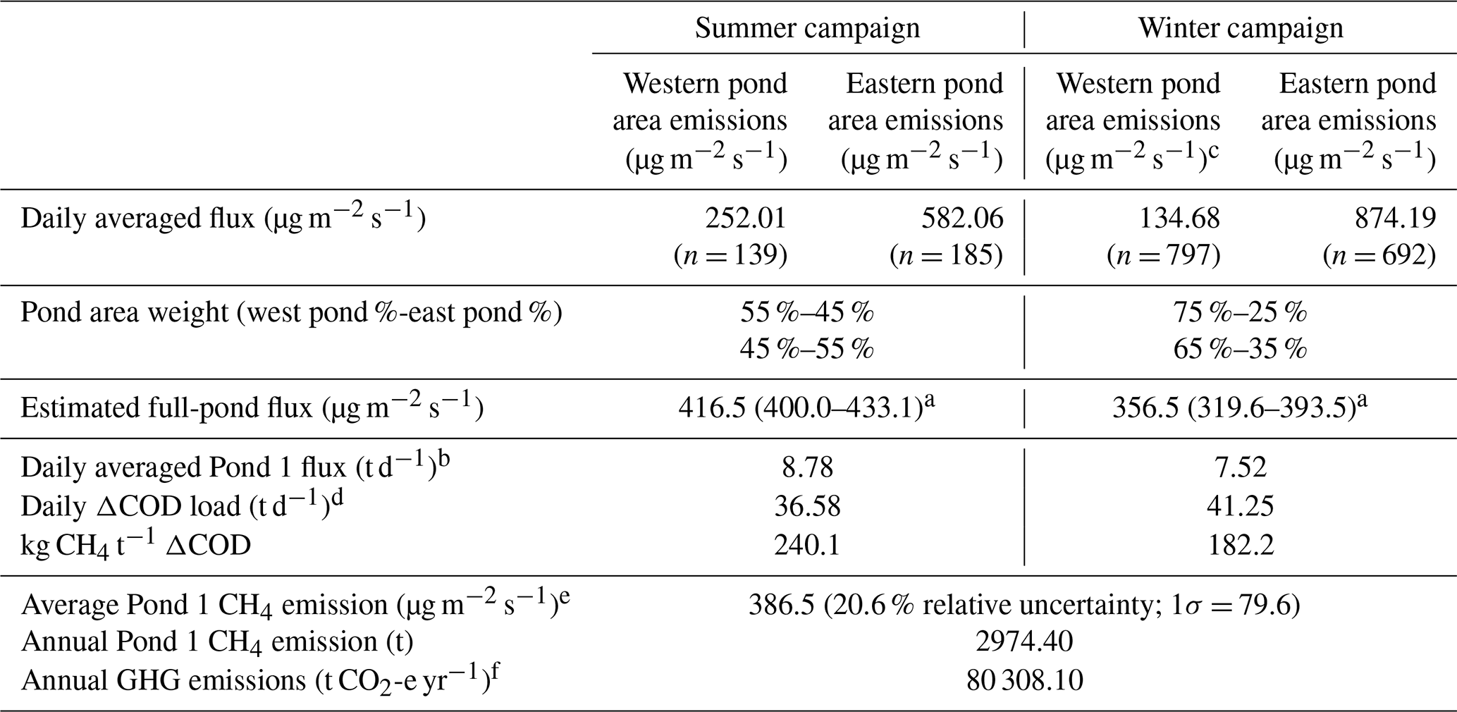
^a Range inside brackets are obtained by varying the weights associated with the pond area measured by each laser. We varied the weight by ±5 % relative to the mean (for the summer campaign: low estimate is west pond 55 %-east pond 45 % and high estimate 45 %–55 %; for winter campaign: low estimate is west pond 75 %-east pond 25 % and high estimate 65 %–35 %; see Sect. 2.6). ^b The 25W Pond 1 area is 244 007 m². ^c n – the number of good measurements. ^d COD – chemical oxygen demand. The mean daily net load of COD (ΔCOD) is 379.8, 306.2 mg L⁻¹ for winter and summer campaign, respectively. ΔCOD is determined by the difference between the average influent COD value measured at the east end and the average wastewater COD value at the outlet, ΔCOD_summer = 445.0 − 138.8 = 306.2 mg L⁻¹, ΔCOD_winter = 581.3 − 201.4 = 379.8 mg L⁻¹. Daily flow rate is 108.6, 119.5 ML d⁻¹ for winter and summer campaign, respectively. The daily net load of COD in t d⁻¹ = 379.8 × 10⁻⁹ mg L⁻¹ × 108.6 × 10⁶ L d⁻¹ = 41.25 t COD d⁻¹ (winter campaign). For summer campaign, the daily net load of COD in t d⁻¹ = 306.2 × 10⁻⁹ mg L⁻¹ × 119.5 × 10⁶ L d⁻¹ = 36.58 t COD d⁻¹. ^e Total relative uncertainty associated with the averages is 20.9 % and 20.4 % for the winter and summer measurements, respectively. The total relative uncertainty for both campaigns is 20.6 % using the equation: square root of (0.5 × (20.9 %)² + 0.5 × (20.4 %)²) and is dominated by the inverse dispersion model uncertainty. The 1σ value was calculated using the definition for the coefficient of variation to represent the relative uncertainty (CV = σ $/$ mean). Solving for sigma gives: 1σ = CV × mean = 79.6 µg m⁻² s⁻¹. ^f Annual Pond 1 emission (t) × 27 of global warming potential for CH₄.

The total relative uncertainty of the full-pond flux was calculated to be 20.4 % and 20.9 % for the summer and winter measurement, respectively, and the total mean relative uncertainty for both campaigns was calculated to be 20.6 % using the equation: square root of (0.5 × (20.9 %)² + 0.5 × (20.4 %)²). Therefore Pond 1 flux was 416.5 µg m⁻² s⁻¹ (20.4 % relative uncertainty) in summer and 356.5 µg m⁻² s⁻¹ (20.9 % relative uncertainty) in winter. The average emission for Pond 1 over the two campaigns is 386.5 µg m⁻² s⁻¹ (20.6 % total mean relative uncertainty, 1σ = 79.6 µg m⁻² s⁻¹) (Table 1).

Methane emissions from Pond 1 showed temporal and spatial variations over the measurement periods, with an average of annual Pond 1 CH₄ emission of 2974 t (Table 1). The annual CH₄ emission was then calculated as CO₂ equivalent (CO₂-e) by multiplying this value by a factor of 27 (CH₄'s global warming potential in 100 years) based on IPCC report (2021), resulting in an annual GHG emission of 80 308 t CO₂-e yr⁻¹ in 2024/25 (Table 1). The emissions at the eastern pond area were comparable to the measurements from wastewater treatment facilities in the US using remote sensing techniques (Thorpe et al., 2021).

According to the daily average effluent flow of 108.6 ML d⁻¹, we calculated net daily COD change in Pond 1 (ΔCOD, mg L⁻¹) using the difference in the COD value between the average influent COD value (measured at the east end) and the average effluent COD value at the outlet. The ΔCOD for the summer and winter campaign was 306.2 and 379.8 ML d⁻¹, corresponding to 36.58 and 41.25 t COD d⁻¹ processed by the Pond 1, respectively. Therefore, the accumulative CH₄ flux per t COD change accounted for 182.2 kg CH₄ t⁻¹ ΔCOD for winter campaign, comparable to the value of 240.1 kg CH₄ t⁻¹ ΔCOD for summer campaign (Table 1).

Table 2 Flux measurements from this study compared to NGERS reporting, the mass balance of liquid emission and methane production from the anaerobic Pot.

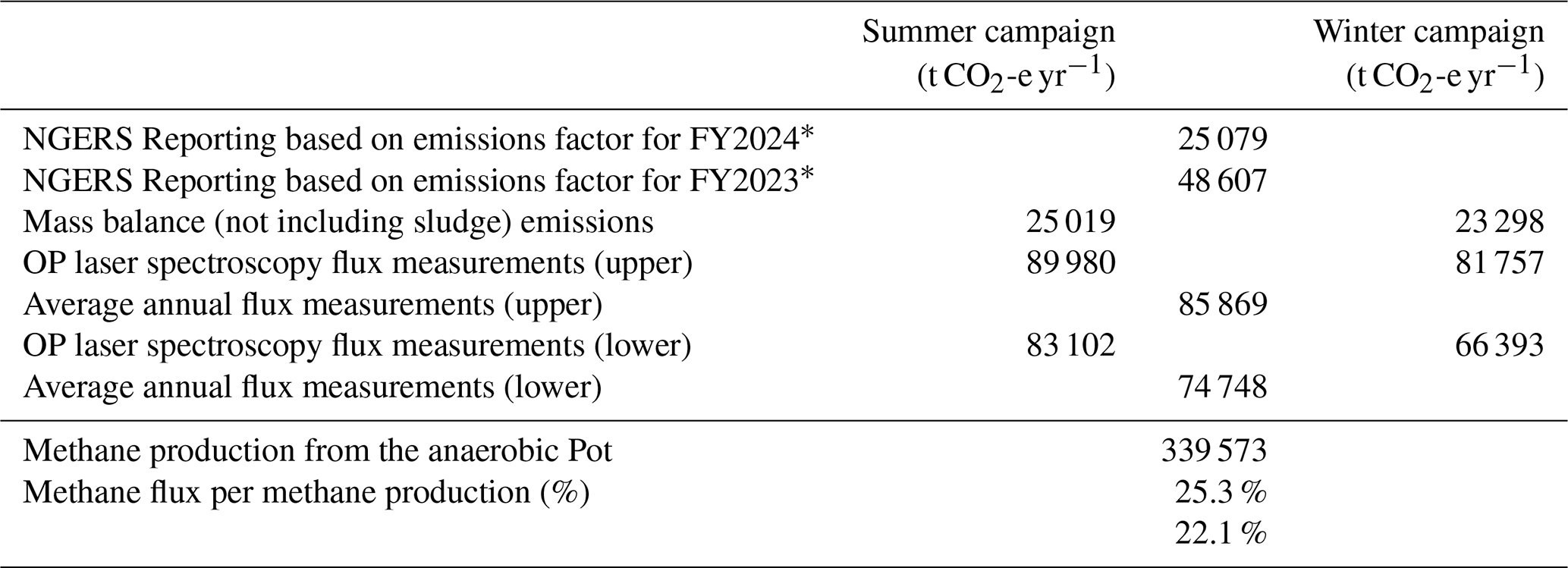
^∗ NGERS, national greenhouse and energy reporting scheme.

The average annual flux as a proportion of CH₄ production ranged from 22.0 % to 25.3 %, reflecting that the measured emissions are approximately 25 % of the CH₄ captured by the anaerobic Pot. Our measurements are ∼ 2.0–2.3 times higher than the NGERS reported emissions from Pond 1 (adopting the emissions factor of Unmanaged Aerobic Lagoon, Method 2, NGERS) which averaged 36 843 t CO₂-e yr⁻¹ for financial years 2023 and 2024 (Table 2). These results are comparable to other studies on CH₄ emissions from WWTPs, which found that measured emissions were almost 2 times IPCC (Intergovernmental Panel on Climate Change)/EPA estimates that use emission factors (Moore et al., 2023; Song et al., 2023).

In Australia, there are over 1200 WWTPS; only a few primarily use treatment ponds that are similar to our study. Climate-change calculations should not overlook the potentially underestimated CH₄ emissions. In fact, while fugitive CH₄ emissions from coal, oil, and gas plants have been the focus in Australia and globally, little attention has been paid to CH₄ emissions from sewage treatment ponds. Meanwhile, climate change-induced warming in Australia and Melbourne's growing population will likely enhance CH₄ emissions from WWTPs. These issues must be addressed, and concrete actions to reduce GHG emissions from the wastewater sector are urgently needed.

4 Conclusions and recommendations

Methane emissions from 25W Pond 1 showed the temporal and spatial variations over the measurement periods. The average annual flux as a proportion of CH₄ production ranged from 22.0 % to 25.3 %, reflecting that the measured emissions are approximately 25 % of the methane captured by the Pot. Our measurements are ∼ 2 times higher than the NGERS estimate. We therefore recommended that the options for mitigating CH₄ emissions include examining the impacts of changing management practices. Such practices could involve increasing the dredging frequency of Pond 1, increasing the efficacy of capturing CH₄ from the covered area (e.g., by extending its length), optimizing the aerator operating time to prolong the period that dissolved methane remains in the wastewater, or adding substances to the pond (e.g. microalgae). However, in practice these proposals might not be viable options. In the long run, to substantially reduce fugitive CH₄ emissions from WWTPs that contributes to achieving carbon neutrality, it will be necessary to implement a new primary treatment plant and move away from the current anaerobic treatment followed by aerobic pond design.

In addition, this study has shown that inverse-dispersion modelling combined with open-path spectroscopic techniques are useful tools to continually monitor emissions at a large scale. Measuring a suite of gas emissions including CH₄, N₂O, and NH₃, would better allow the development of effective mitigation strategies. This is especially important once the methane oxidizers and producers in a wastewater treatment pond are identified.

Appendix A: Abbreviations

BOD	biological oxygen demand
COD	chemical oxygen demand
IDM	inverse-dispersion modelling
NGERS	National Greenhouse and Energy Reporting Scheme
OPL	open-path laser
WWTPs	wastewater treatment plants