Stratospheric aerosol measurements using a Frequency Scanning Lidar method

We present a method to derive stratospheric aerosols up to 30 km from Frequency Scanning Lidar (FSL) measurements. The lidar itself is designed as a universal instrument for the middle atmosphere and is capable of doing Doppler-Mie, Doppler-Rayleigh and Doppler-resonance measurements, for simultaneous retrievals of wind, temperature and aerosols. The system leverages a narrowband Alexandrite ring laser operating at the 770 nm potassium (K) line with a 3.3 MHz spectral width and high-resolution spectroscopy. By scanning a 100 MHz spectral window with sub-MHz sampling, the filter chain efficiently suppresses the Rayleigh background and spectrally resolves the Mie peak, enabling the separation of aerosol and molecular scattering. The FSL method's solar-blind Mie channel allows for measurements both day and night, while its compact design (approximately one cubic meter in volume) facilitates mobile deployment. With a vertical resolution of 200 m and a temporal resolution of 20 min, as achieved for the data presented here using the instrument configuration described in this study, the FSL method provides high-resolution observations of aerosol distributions in the stratosphere. The uncertainties of the FSL method for the backscatter coefficient are approximately $\mathrm{1.5}\times {\mathrm{10}}^{-\mathrm{10}}$ m⁻¹ sr⁻¹ at 20 km, both during day and night. We demonstrate the method's capabilities by presenting backscatter coefficient profiles measured during selected periods from 2022 to 2024. These profiles show good agreement with satellite-derived profiles from the Ozone Mapping and Profiler Suite Limb Profiler (OMPS-LP) and the Stratospheric Aerosol and Gas Experiment on the International Space Station (SAGE III/ISS) with a mean absolute deviation of ∼25 % at altitudes of 15–25 km. This demonstrates the potential of the FSL method for providing high-resolution, long-term observations of stratospheric aerosols.

1 Introduction

Stratospheric aerosols play an important role in the Earth system because they strongly influence both climate and atmospheric chemistry (e.g. Kremser et al., 2016). By scattering and absorbing solar and terrestrial radiation, they modify the planetary energy balance, cooling the surface while warming the lower stratosphere, and thereby altering atmospheric circulation patterns. Episodic injections from large volcanic eruptions can produce radiative forcing (e.g. Robock and Mao, 1995) comparable to anthropogenic greenhouse gases on short timescales, offering natural experiments for testing climate models and, controversially, informing proposals for solar radiation management (e.g. Crutzen, 2006). At the same time, stratospheric aerosol particles provide surfaces for heterogeneous chemical reactions that affect ozone concentrations (e.g. Fahey et al., 1993), with implications for ultraviolet radiation reaching the surface and for compliance with international agreements such as the Montreal Protocol. Because their properties are shaped by a combination of emissions, microphysical processes, and large-scale transport, stratospheric aerosols also serve as sensitive tracers of dynamical variability, making them key observables for understanding past, present, and future changes in the climate system.

In volcanically quiet periods, the stratospheric aerosol layer is primarily formed by the vertical transport of aerosols and precursor gases such as carbonyl sulphide (OCS) and sulphur dioxide (SO₂) bottom up through the tropical tropopause layer (Kremser et al., 2016). Aerosols or aerosol-forming substances can be injected directly into the stratosphere, particularly by explosive volcanic eruptions, but in recent years also increasingly by wildfire-driven pyrocumulonimbus clouds (Fromm et al., 2010). The sulphur compounds injected into the stratosphere are converted into sulphuric acid (H₂SO₄), which combines with H₂O to form sulphate aerosols. The produced sulphate aerosols are known to exist at 15 to 25 km altitude (Junge et al., 1961), often referred to as the “Junge layer”. Depending on altitude, latitude, and season, there is a very high variability in stratospheric aerosol. There is also top-down particle input from space into the stratosphere. This occurs naturally through meteoric smoke particles (MSPs) (e.g. Plane, 2012) or, increasingly, anthropogenically through satellite debris (e.g. Murphy et al., 2023). MSPs form from the ablation of meteoroids at an altitude of 70–120 km (Plane, 2003) and pass through the mesosphere into the stratosphere. Initially, MSPs are thousands of times smaller than stratospheric sulphate aerosols (Hunten et al., 1980), but models predict that they may grow to radii of around 40 nm as they descend (Plane, 2012).

A common method for observing stratospheric aerosols is using spaceborne spectrometers. Depending on the viewing geometry, the transmitted or scattered solar radiation is measured and the aerosol extinction coefficient or aerosol optical depth is derived. This makes it possible to achieve near-global coverage. Depending on the exact measurement methodology, problems arise that need to be solved, such as the correct quantification of the absorption contributions of ozone, nitrogen dioxide and water vapour, as well as molecular scattering (e.g. SAGE III ATBD Team, 2002) or, for limb scattering measurements, the need to make assumptions about the influence of multiple scattering and aerosol properties (e.g. von Savigny et al., 2015; Rozanov et al., 2024). Moreover, it is possible to get aerosol information up to the mid-stratosphere (about 35 km) by balloon-borne in situ measurements (e.g. Deshler et al., 2003). However, these soundings are rare and limited to appropriate launch sites.

Ever since the launch of the Cloud-Aerosol Lidar and Infrared Pathfinder Satellite Observation (CALIPSO) in 2006 (Winker et al., 2009) with its Cloud-Aerosol Lidar with Orthogonal Polarization (CALIOP), spaceborne lidars have also been playing an increasingly important role in the global measurement of aerosols in the troposphere and lower stratosphere. The importance of spaceborne lidars, which are particularly notable for their high spatial coverage, has increased further in recent years through High Spectral Resolution Lidar (HSRL) satellite missions using the instruments Atmospheric LAser Doppler INstrument (ALADIN) (Stoffelen et al., 2005), ATmospheric LIDar (ATLID) (Gelsthorpe et al., 2017) and Aerosol and Carbon Detection Lidar (ACDL) (Dai et al., 2024).

High-resolution ground-based lidar measurements of stratospheric aerosols are highly valuable, as they provide vertically resolved long-term observations that complement satellite and aircraft measurements and thereby contribute to a more robust assessment of the global distribution and radiative forcing of stratospheric aerosols (Trickl et al., 2024; Sakai et al., 2025). This makes it possible, for example, to monitor the development and characteristics of wildfire smoke events in the stratosphere (Baars et al., 2019; Hu et al., 2019; Ohneiser et al., 2022). Their fine vertical resolution is crucial for resolving sharp gradients near the tropopause, thin aerosol layers, and small-scale structures associated with gravity waves and transport. Such features can exert a disproportionate influence on radiative effects and heterogeneous chemistry, yet they are often inadequately represented or entirely missed in coarser satellite retrievals and climate model outputs.

Extending lidar measurements to at least 30 km altitude is essential for resolving the full vertical extent of the Junge layer, capturing lofted aerosol from moderate and large volcanic eruptions or wildfires, and detecting faint signals potentially linked to MSPs or re-entering space debris. They provide critical benchmarks for evaluating climate models, interpreting satellite aerosol products, and attributing observed stratospheric aerosol variability to natural and anthropogenic drivers. Despite these needs, most current ground-based lidar systems lack the sensitivity required to detect stratospheric aerosols above the Junge layer (Langenbach et al., 2019; Chouza et al., 2020). This limitation results from the limited laser power and the spectral properties of the lidar system, which lead to an insufficient signal-to-noise ratio at high altitudes, where Rayleigh scattering from air molecules dominates the return signal. Under non-volcanic (background) conditions, the weak backscatter of stratospheric aerosols at conventional wavelengths (e.g. Nd:YAG 532 nm) further hampers detection. In contrast, the use of a longer wavelength, for example 770 nm, significantly reduces Rayleigh dominance over particle scattering. Combined with the Frequency Scanning Lidar (FSL) method presented in the next chapter, this enables precise monitoring of stratospheric aerosol structures with high vertical and temporal resolution, even under fluctuating environmental conditions during day and night. The system is designed for worldwide mobile deployment and long-term continuous operation. Its optical design allows measurements under both daytime and nighttime conditions, including the continuous solar illumination encountered during the polar summer.

The paper is structured as follows: Sect. 2 presents the methodology and operational principles of the FSL approach, with emphasis on its ability to provide high-resolution aerosol data under daylight conditions. The results are shown in Sect. 3. Section 4 discusses the resulting time series of FSL-derived aerosol parameters and compares it with collocated satellite observations. Section 5 summarises the main findings and provides an outlook on future developments.

2 Methodology

2.1 Determination of particle backscatter coefficient with conventional lidar instruments

Stratospheric aerosol measurements traditionally rely on separating molecular (Rayleigh) and particle (Mie) backscattered signals at a single wavelength to retrieve particle backscatter coefficients using a reference profile (e.g. Fernald, 1984). In the simplest form, this reference is constructed by extrapolating a pure Rayleigh signal under the assumption that the atmosphere above approximately 30 km is free of aerosol. The Rayleigh reference is then extended downwards, and deviations are attributed to aerosol backscatter. However, this approach is sensitive to uncertainties in the assumed molecular backscatter profile due to atmospheric temperature and density variations. Despite this limitation, it remains widely used due to its simplicity and low hardware requirements.

An improved approach involves the use of additional wavelength-shifted Raman scattering (Schneider and Eixmann, 2002). Since Raman scattering occurs exclusively on molecules, it provides an aerosol-independent backscatter signal as a reference signal. A major disadvantage of this measurement method is the small backscattering cross-section of the Raman scattering, which is 3 orders of magnitude lower than for Rayleigh scattering. This results in a drastically decreased return signal for the Raman scattering, leading to a need for instruments with large telescopes and powerful lasers for observations in the stratosphere. Another limitation arises from the requirement for separate detectors and optical paths for the Rayleigh and Raman channels. These can introduce systematic errors due to detector-specific nonlinearities (e.g., varying dead times) on the different optical paths.

HSRL techniques overcome limitations of standard backscatter lidar by employing a dual-channel detection. In this configuration, the backscattered light is split between two detectors, with one channel equipped with a high-precision, narrowband spectral filter. The narrowband laser is then stabilized to the filter, which possesses a spectral width significantly narrower than the Rayleigh-scattering spectrum. By suppressing a specific portion of the return signal the filter enables the system to isolate the particulate (Mie) and molecular (Rayleigh) components. The aerosol optical properties are then derived directly from the intensity ratio of the signals recorded by the two detectors. Typical filter implementations use interferometers, such as Fabry-Perot interferometers, or molecular absorption cells, such as iodine vapor cells (Shipley et al., 1983; Sroga et al., 1983; Hair et al., 2008). For these instruments, the Doppler shift induced by atmospheric motion must be accounted for by ensuring the filter bandwidth is wide enough to encompass the maximum expected shift. Additionally, the laser linewidth must be maintained substantially below the filter width to ensure consistent measurement accuracy. For ESA’s Aeolus mission, which aimed primarily at global wind profiling, this challenge was addressed by using a Fizeau interferometer as a filter (Stoffelen et al., 2005). This allowed the implementation of a fringe-imaging technique on a multi-pixel detector to simultaneously measure the Doppler shift for wind retrieval and account for it during aerosol analysis. In contrast, the subsequent ESA–JAXA EarthCARE mission returned to a classical HSRL architecture for its ultraviolet ATLID (Gelsthorpe et al., 2017; Wehr et al., 2023). Since EarthCARE's primary objective is the characterization of clouds and aerosols rather than direct wind measurements, the HSRL technique provides a more direct means of retrieving vertical aerosol profiles and particle-type discrimination via depolarization analysis (Donovan et al., 2024).

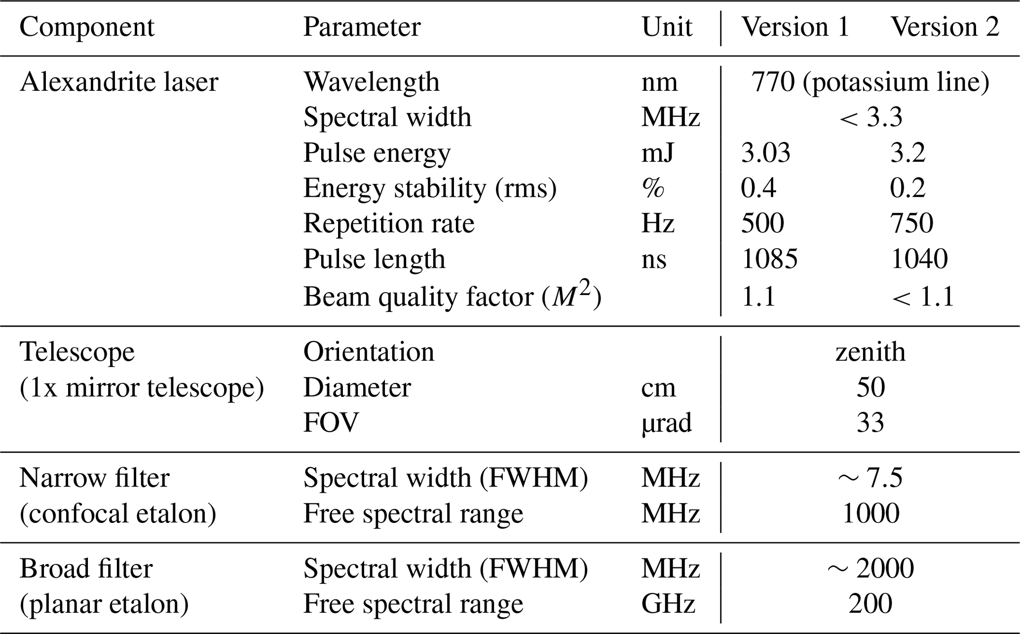
Lidars have been developed at the Institute of Atmospheric Physics (IAP) for many years. In addition to the RMR lidar systems used in Kühlungsborn (Northern Germany) and Andenes (Northern Norway), we have developed a lidar system for many years that utilizes a FSL method with a new generation of Alexandrite laser (Munk et al., 2018). The FSL method used in this study is designed to sample multiple frequencies within a very short time by changing the laser frequency from pulse to pulse, which allows a reduction of the combined spectral bandwidth of the laser and the detection filters. This method was originally developed at IAP for Doppler resonance measurements at 770 nm to determine potassium density and neutral temperatures with high precision in the mesopause region (about 80 to 105 km) (Höffner and Lübken, 2007). With the lidar presented in this publication, the FSL method is used to derive atmospheric winds and temperatures simultaneously to the aerosol retrievals shown in this work (Mense et al., 2024; Mense, 2025). The tuning of the narrowband Alexandrite laser to the D1 transition of potassium at 769.9 nm also allows for simultaneous measurements of resonance scattering between 80 and 100 km altitude. Aerosol retrievals using the FSL method benefit from the narrowband properties of the used Alexandrite laser and filters in the form of a high sensitivity even in daylight conditions. In addition to the advantages offered by the method for aerosol measurements, the instrument’s design as a universal lidar is the main reason for using the frequency-scanning method, despite the existence of simpler methods for the retrieval of atmospheric aerosol measurements (Lübken and Höffner, 2021). The current VAHCOLI system configuration includes a dedicated depolarization channel. Since this channel was not yet operational during the measurements presented in this study, depolarization data are not included in the present analysis. Future measurements will use this channel to provide additional information on aerosol particle shape. Appendix Table A1 provides an overview of the lidar parameters of the VAHCOLI system used in this study.

2.2 Determination of backscatter ratio and backscatter coefficient with FSL method

2.2.1 FSL method

The FSL method of the lidar system VAHCOLI (Vertical And Horizontal COverage by LIdar) presented here uses a spectroscopic measurement method developed at the IAP (Lübken and Höffner, 2021), which has already been used successfully in the IAP potassium Doppler-resonance lidar in the past (von Zahn and Höffner, 1996). This has been further developed recently (Froh, 2021) and adapted for the FSL measurement system. The FSL method relies on the following key elements:

1. Narrowband Laser Emission: A highly narrowband Alexandrite ring laser with a wavelength of 770 nm and a spectral width of 3.3 MHz is utilized, featuring a spectral linewidth much smaller than the Rayleigh scattering bandwidth (approximately 1400 MHz) and close to the bandwidth of Mie scattering with a linewidth typically <0.1 MHz. This ensures exceptional frequency purity, favouring spectral precision over short pulse duration. The two available laser configurations used are power-scaled versions running at 500 and 750 Hz repetition rate with 3.03 and 3.2 mJ pulse energy, respectively. They are described in detail in Munk et al. (2023) and have been developed in close collaboration with the Fraunhofer Institute for Laser Technology in Aachen over the past decade (Strotkamp et al., 2013; Munk et al., 2021).

2. Spectral Scanning Capability: The laser wavelength is tuned pulse-to-pulse around 770 nm, covering the full spectral range relevant for Mie scattering while scanning only a narrow (∼100 MHz) fraction of the Doppler-broadened Rayleigh spectrum, required to account for wind-induced Doppler shifts at inclined lines of sight. This frequency-scanning approach is achieved using a fast and precise tuning mechanism in the Alexandrite ring laser, operating in combination with a highly stabilized filter (Froh, 2021).

3. Daylight Operation via Solar Background Suppression: To enable reliable measurements under full daylight conditions, the instrument incorporates narrowband filtering using a combination of planar (∼2000 MHz) and confocal (∼7.5 MHz) etalons. By doing so, solar background radiation is significantly suppressed, enhancing signal-to-noise performance during daytime operations and rendering the Mie channel effectively solar-blind (Froh, 2021).

4. Spectral Separation of Mie and Rayleigh Scattering: The backscattered signal is optically separated into distinct Mie and Rayleigh components using the confocal etalon mentioned above, precisely matched to the spectral widths of the respective scattering processes, as schematically shown in Fig. 1. This spectral splitting enables independent detection of the Mie signal with strongly suppressed Rayleigh interference, while maintaining simultaneous and accurate measurement of both scattering contributions (Froh, 2021; Mense et al., 2024).

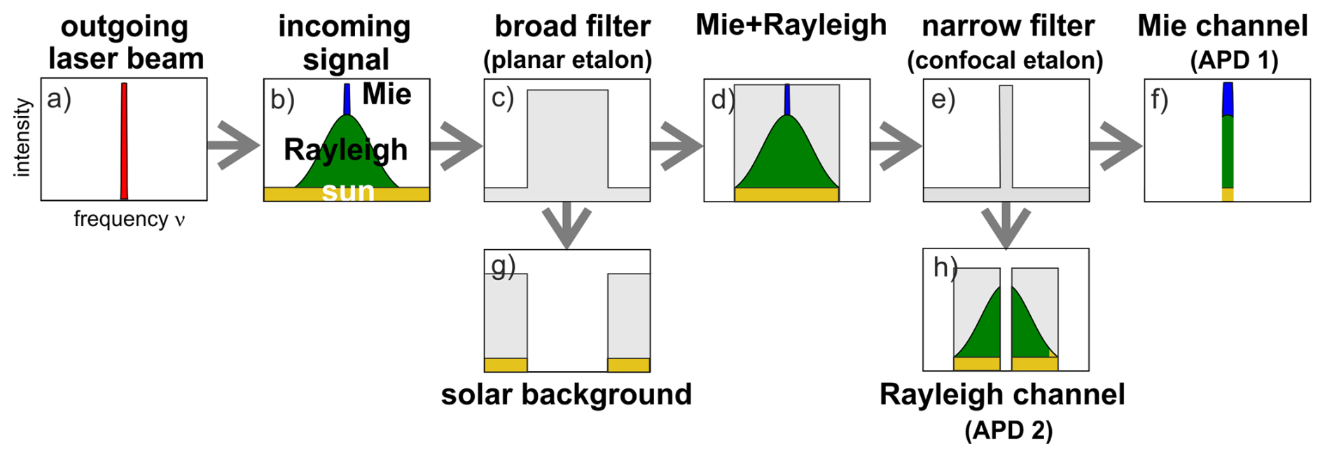
Figure 1 Simplified and idealized schematic of the emission of a single narrowband laser pulse (a), and the subsequent spectral splitting of the backscattered laser pulse signal together with the spectral suppression of solar background radiation. (b–h) The separation of the backscattering processes is based on the Doppler width, illustrated with Mie (blue) and Rayleigh (green) scattering, a solar background (yellow), and an idealized rectangular filter (planar and confocal etalon).

The combination of these four principles of the FSL method result in the measurement of high-resolution spectra of the backscattered signal, as described in more detail in Lübken and Höffner (2021). Actually measured spectra from both channels are shown in Fig. 2 for a case with a cirrus cloud. The spectral shape is a result of the convolution of the spectra of scanning lidar, filters and atmospheric backscatter and therefore differs from the strongly idealized filters shown in Fig. 1. It should be noted that the avalanche photodiode (APD) itself is not a frequency-tunable detector like a spectrometer. The spectral resolution is obtained from the scanning laser (which requires a complex deconvolution of the various spectra). Due to the strong aerosol load in the cirrus cloud, a dip is seen in APD2, where the aerosol signal is transmitted through the confocal etalon, for weaker aerosol loads this dip is almost invisible. These captured spectra can then be further processed for precise measurements of the line of sight wind as described in Mense et al. (2024) and aerosol parameters, as described in this publication.

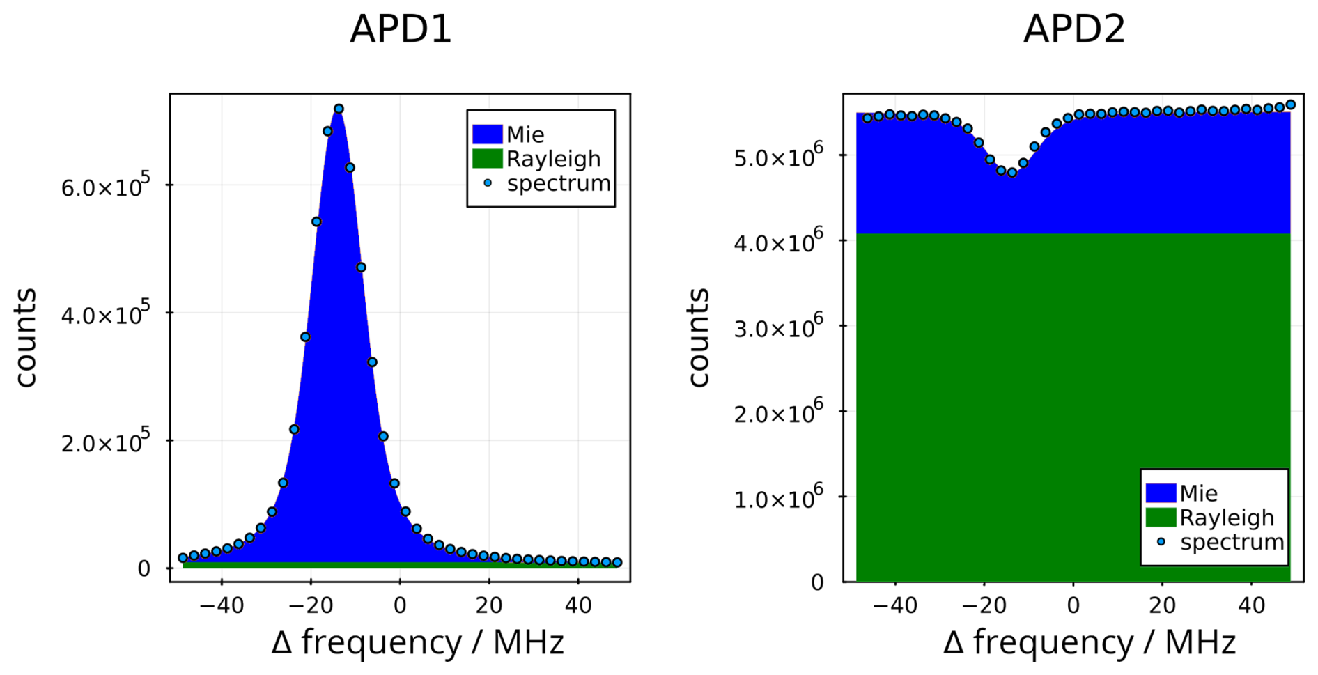
Figure 2 Example of spectra measured with APD1 (left) and APD2 (right) in 10±0.5 km altitude on the 8 February 2023 at 00:00 UTC in a cirrus cloud. The abscissa denotes the frequency offset of the laser. The signal of APD1 peaks at a frequency that equals the wind-induced Doppler shift of the backscattered light. The estimated contributions of Mie- and Rayleigh-scattering are color coded. Here the background from the sun and the dead count rate is assumed to be negligible, since the signal is high and the measurement was done at night.

Since the spectral shape of laser and filters are permanently measured using internal references, the backscatter ratio (BSR, or R_Aer) can be derived from the measured atmospheric spectra. Subsequently, the corresponding backscatter coefficient (BSC, or β_Aer) is determined, providing a quantitative measure of the aerosol scattering properties of the atmosphere.

2.2.2 Aerosol data processing

Backscatter ratio

The backscatter ratio (BSR), $R_{\mathrm{Aer}}={\mathit{\beta }}_{\mathrm{Total}}/{\mathit{\beta }}_{\mathrm{Mol}}$, quantifies the relative contributions of Mie and Rayleigh scattering (Fernald, 1984). The altitude-dependent BSR, R_Aer(z), is given by:

$$\begin{array}{}\text{(1)}& R_{\text{Aer}}\left(z\right)={\displaystyle \frac{{\mathit{\beta }}_{\text{Aer}}\left(z\right)+{\mathit{\beta }}_{\text{Mol}}\left(z\right)}{{\mathit{\beta }}_{\text{Mol}}\left(z\right)}}={\displaystyle \frac{{\mathit{\beta }}_{\text{Aer}}\left(z\right)}{{\mathit{\beta }}_{\text{Mol}}\left(z\right)}}+\mathrm{1}\end{array}$$

where β_Aer(z) and β_Mol(z) are the altitude-dependent aerosol and molecule backscatter coefficients.

For pure molecule scattering, R_Aer=1. When aerosol scattering is present, R_Aer>1, and R_Aer−1 quantifies the ratio of aerosol to molecular backscatter. The concept for the retrieval of the Mie and Rayleigh signals from the spectrum, necessary for the calculation of the backscatter ratio, is shown in Fig. 3. Panel (a) shows the spectrum measured with APD1, normalized to the maximum intensity at every altitude for the sake of visibility.

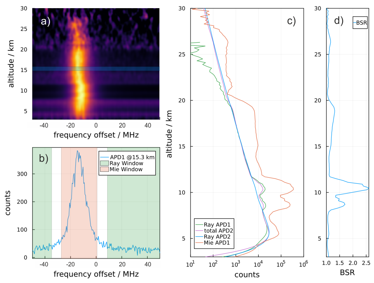
Figure 3 Connection between measured spectra with FSL method and determined BSR. (a) Example of an atmospheric spectrum measured using APD1 on 28 February 2023 between 19:30 and 22:30 UT with the vertical pointing telescope. A vertical integration window of 1 km was used, which was shifted in 200 m steps. (b) Spectrum measured on APD1 in 15.3±0.5 km. The windows used for the retrieval of the Mie and the Rayleigh signal are marked in orange and green. (c) Signals retrieved from the spectra used for the calculation of the BSR. (d) calculated BSR profile. See text for information on normalization, corrections, and channel crosstalk.

The Mie channel (APD1) contains the narrowband spectrum of the Mie and Rayleigh signals transmitted through the confocal etalon, with their relative contributions varying with the instantaneous laser wavelength across the scanned spectrum, together with the APD dark count rate and a solar background contribution that is smaller than the dark count rate. The Rayleigh channel (APD2) detects only the fraction of the lidar signal that is reflected by the confocal etalon and coupled out via a beam splitter in the return path. Note that the physically implemented spectral separation of the Mie and Rayleigh signals described here was previously illustrated in an idealized manner in Fig. 1 (e, f, and h). Consequently, the detected signal at APD2 does not represent the full Rayleigh scattering, as a small Rayleigh contribution is transmitted through the confocal etalon and therefore not captured in this channel. In addition to the reflected Rayleigh component, the signal contains contributions from Mie scattering, solar background radiation, and the intrinsic dark count rate of the APD (Froh, 2021).

In principle, aerosol load can be determined by comparing the peak of the spectrum measured using APD1 to the wings of the spectrum, which requires only a single APD and thus reduces instrumental complexity and potential sources of systematic error compared to multi-detector approaches. In the absence of aerosol, the spectrum is flat (Rayleigh background only). Peaks above this background indicate Mie backscatter. For higher altitudes, the presented BSR retrieval still uses additional information from the APD2 spectra (dark counts and solar background removed) to mitigate the low transmission of Rayleigh signal onto APD1, as explained below.

Mie and Rayleigh signals are extracted from APD1 using three windows, as shown in Fig. 3b. For each altitude bin the window position and width are calculated based on the Voigt-fit results used for the wind measurement, as discussed in Mense et al. (2024). The centre window (red) has a width of two times the Mie peak's FWHM (Full Width Half Maximum), and thus contains most of Mie photons (P_1,c). The outer windows (green) have a cumulative width of four times the Mie peak's FWHM and are used to determine the Rayleigh background P_1,Ray (green). The Mie signal then is:

$$\begin{array}{}\text{(2)}& P_{\mathrm{1},\text{Mie}}=P_{\mathrm{1},c}-P_{\mathrm{1},\text{Ray}}\end{array}$$

Due to the suppression of Rayleigh scattering in the APD1 channel, the Rayleigh signal becomes too noisy above typically 20 km, as visible in Fig. 3c. In this case we need to use APD2 instead, as it retains Rayleigh backscatter. From the spectrum measured with APD2, P_2,total is retrieved using the same window method described before. For processing P_2,total is normalized to P_1,Ray at 15 km altitude.

The BSR is initially estimated as:

$$\begin{array}{}\text{(3)}& R_{\text{Aer}}\left(z\right)={\displaystyle \frac{P_{\mathrm{1},\text{Mie}}\left(z\right)}{P_{\mathrm{2},\text{total}}\left(z\right)}}\cdot {\displaystyle \frac{\mathrm{1}}{\mathit{\zeta }\cdot \mathit{\eta }\left(z\right)}}+\mathrm{1}\end{array}$$

where ζ and η(z) are two correction factors that account for the optical setup and the digital signal processing, respectively. The factor ζ represents the suppression of the Rayleigh signal in APD1 relative to the Mie transmission, defined by the transmission ratio $\mathit{\zeta }=t_{\text{Mie}}/t_{\text{Ray}}$. This suppression is a direct consequence of the spectral filter setup within the instrument's optical design. It can either be calculated numerically using the measured filter functions of the planar and confocal etalon, or determined experimentally using thin cirrus clouds. In the setup shown in this publication, ζ is determined experimentally to be around 60. The altitude-dependent factor η(z) is calculated dynamically from the discrete window width and the Voigt-fit results for each altitude channel to avoid numerical artifacts. The measured spectrum is a Voigt profile, resulting from the convolution of the laser spectrum, the atmospheric backscatter, and the instrument's filter function. Due to the finite number of channels, any shift or deformation of this distribution within the processing window (e.g., due to atmospheric turbulence) alters its shape. Thus, η(z) accounts for both the ratio between the fitted Mie peak height and the mean photon count in the center window, as well as the fraction of photons not captured within the finite window width.

Since P_2,total includes both Rayleigh and Mie contributions, R_Aer is systematically underestimated. An iterative approach is thus used, in which P_2,total is corrected with the calculated R_Aer

$$\begin{array}{}\text{(4)}& P_{\mathrm{2},\text{Ray}}={\displaystyle \frac{P_{\mathrm{2},\text{total}}}{R_{\text{Aer}}}}.\end{array}$$

This can then be used to calculate R_Aer again:

$$\begin{array}{}\text{(5)}& R_{\text{Aer}}\left(z\right)={\displaystyle \frac{P_{\mathrm{1},\text{Mie}}\left(z\right)}{P_{\mathrm{2},\text{Ray}}\left(z\right)}}\cdot {\displaystyle \frac{\mathrm{1}}{\mathit{\zeta }\cdot \mathit{\eta }\left(z\right)}}+\mathrm{1}\end{array}$$

This iterative correction quickly converges to the true R_Aer (typically ≪10 iterations), which is shown in Fig. 3d and leads to the pure Rayleigh signal, shown in blue in Fig. 3c.

Backscatter coefficient

The BSR is a convenient relative diagnostic of aerosol contributions but suffers from its dependence on the background molecular profile, which varies with altitude, season, and atmospheric state. This dependence limits its use for model validation and long-term monitoring, as changes in BSR may partly reflect variations in the reference atmosphere rather than genuine aerosol variability. By contrast, the aerosol backscattering coefficient (BSC, denoted as β_Aer(z,λ) in Eq. 6) is an absolute, physically consistent measure of aerosol scattering. When particle size information is available, it can be compared across datasets, models, and time periods. Its use therefore provides a more reliable basis for geophysical interpretation, long-term trend analysis, and the evaluation of model performance.

To obtain the BSC from the BSR, we use the following relation resulting from Eq. (1):

$$\begin{array}{}\text{(6)}& {\mathit{\beta }}_{\text{Aer}}(z,\mathit{\lambda })={\mathit{\beta }}_{\text{Mol}}(z,\mathit{\lambda })\cdot \left(R_{\text{Aer}}\right(z,\mathit{\lambda })-\mathrm{1})\end{array}$$

β_Mol(z,λ) can be derived for dry air from the density profile N(z) and the molecular backscattering cross-section ${\mathit{\sigma }}_{\mathit{\pi }}^R\left(\mathit{\lambda }\right)$ (Measures, 1984):

$$\begin{array}{}\text{(7)}& {\mathit{\beta }}_{\text{Mol}}(z,\mathit{\lambda })=N\left(z\right)\cdot {\mathit{\sigma }}_{\mathit{\pi }}^R\left(\mathit{\lambda }\right)\end{array}$$

with

$$\begin{array}{}\text{(8)}& {\mathit{\sigma }}_{\mathit{\pi }}^R\left(\mathit{\lambda }\right)=\mathrm{5.45}{\left({\displaystyle \frac{\mathrm{550}}{\mathit{\lambda }}}\right)}^{\mathrm{4}}\times {\mathrm{10}}^{-\mathrm{32}}{\text{m}}^{-\mathrm{1}}{\text{sr}}^{-\mathrm{1}}{\text{nm}}^{-\mathrm{4}}\end{array}$$

There are various options for determining the altitude-dependent number density of air molecules. One possibility is to determine it using external sources such as radiosonde ascents or atmospheric models. Another method used here is the direct determination from the molecular signal of the lidar measurement, adjusted using a reference density profile from hourly forecasts of the Integrated Forecasting System (IFS) (cycle 47r3) of the European Centre for Medium‐Range Weather Forecasts (ECMWF) (Copernicus Climate Change Service, 2025a).

The current implementation of the FSL retrieval is limited to aerosol backscatter coefficients. Although extinction could be estimated by assuming a lidar ratio, as in conventional elastic backscatter lidar retrievals, an independent extinction retrieval analogous to HSRL is not yet implemented and is planned for a future extension of the method.

Statistical error of backscatter ratio and backscatter coefficient

The measurement errors given in this publication for the lidar derived backscatter ratio and backscatter coefficient only consider the error of the photon counts, n. For this, we assume a Poisson distribution with a width of ${\mathit{\sigma }}_n=\sqrt{n}$. The error of BSR and BSC are then calculated by feeding the photon count errors through the processing chain using Gaussian error propagation. Resulting errors can thus be considered purely statistical errors. Instrumental and systematic effects are not taken into account for the calculation of the statistical error, due to the difficult estimation of these effects without reliable alternative measurement techniques for comparison. It is important to note here, that due to derivation of the aerosol properties by comparison of signals from the same altitude bin, the method is not affected by the lidar's overlap function (height-dependent overlap between the laser beam and the telescope's field of view (FOV)).

2.3 Determination of backscatter coefficient with satellite instruments

To compare ground-based lidar measurements with data sets from satellites, measurements from the instruments Ozone Mapping and Profiler Suite Limb Profiler (OMPS-LP), Stratospheric Aerosol and Gas Experiment on the International Space Station (SAGE III/ISS) and ATLID are used. A comparison with the spaceborne lidars CALIOP (2006–2023) and ALADIN (2018–2023) appears unsuitable for this work, as the signal above 15 km is too weak in these measurements under background conditions.

The OMPS-LP instrument measures the limb-scattered solar radiation. As with all limb instruments, OMPS-LP is confronted with the challenge that surface reflection and multiple scattering typically make a significant contribution to the total scatter signal, which complicates the methodology. Each measurement not only depends on the aerosol extinction but also on the conditions of the atmosphere and the aerosol microphysical properties. OMPS-LP was launched on 28 October 2011 as the first OMPS mission aboard the Suomi National Polar-orbiting Partnership (S-NPP) satellite into a sun-synchronous orbit at an altitude of approximately 800 km. OMPS-LP is one of three OMPS instruments, alongside two spectrometers with nadir viewing geometry. OMPS-LP/S-NPP has been in operation since February 2012 and is still active today.

The instrument is a prism spectrometer covering a spectral range of 280–1000 nm. Towards the infrared wavelengths, the spectral resolution becomes increasingly coarse (Jaross et al., 2014). The instrument can perform measurements through three vertical slits, which are separated horizontally by 4.25°. The tangent points measured on the ground are approximately 250 km apart. During each measurement, the solar radiance scattered from the atmospheric limb is simultaneously recorded from the ground up to 80–100 km. Approximately 14 orbits, with 160 measurements each, are performed per day. The measurement of a single profile takes approximately 19 s. Global coverage thus takes about 3–4 d.

Using a radiative transfer model, the measured radiances can be converted into aerosol extinction coefficients. For the present study, the “Suomi-NPP OMPS LP L2 AER Daily Product” Version 2.5 from NASA's Goddard Earth Sciences Data and Information Services Center (GES DISC) is used (Taha and Loughman, 2020). The retrieval algorithm is described in Taha et al. (2021). Here, the aerosol extinction coefficient is derived at six wavelength channels (510, 600, 675, 745, 869 and 997 nm) up to a maximum altitude of 40.5 km. All retrievals are independent of each other (Taha et al., 2021).

SAGE III/ISS is a solar occultation instrument (Cisewski et al., 2014). The mission was launched on 19 February 2017 and began collecting data in June 2017. It is an update of the SAGE III instrument on Meteor-3M (Thomason et al., 2010) and is very similar in its functionality. It measures the attenuation of solar radiation due to absorption and scattering on its way through the atmosphere to the instrument during sunrise and sunset events. A scan of a single event takes approximately 30 s to 1 min. The aerosol extinction coefficient is retrieved in nine wavelength channels. Version 6.0 is used for this work (NASA/LARC/SD/ASDC, 2025). This version also includes derived particle size distribution (PSD) parameters according to the method described in Knepp et al. (2024).

The conversion of extinction coefficients derived from satellite instruments into the BSC measured by lidar requires a conversion of the extinction coefficient k retrieved from the satellite measurement to the wavelength of the lidar λ_lidar=770 nm. For this purpose, the Ångström exponent α is calculated for a wavelength combination that is close to the lidar wavelength.

$$\begin{array}{}\text{(9)}& \mathit{\alpha }\left(z\right)=-{\displaystyle \frac{\log \left(\frac{k_{\text{ext}}(z,{\mathit{\lambda }}_{\mathrm{1}})}{k_{\text{ext}}(z,{\mathit{\lambda }}_{\mathrm{2}})}\right)}{\log \left(\frac{{\mathit{\lambda }}_{\mathrm{1}}}{{\mathit{\lambda }}_{\mathrm{2}}}\right)}}\end{array}$$

For OMPS-LP, λ₁=745 nm and λ₂=869 nm are used, for SAGE III/ISS, the wavelengths λ₁=756 nm and λ₂=869 nm are used. The extinction coefficient at 770 nm can now be interpolated using the Ångström exponent α and the extinction coefficient k_ext at one of the two wavelengths.

$$\begin{array}{}\text{(10)}& k_{\text{ext}}(z,{\mathit{\lambda }}_{\text{lidar}})=k_{\text{ext}}(z,{\mathit{\lambda }}_{\mathrm{1}})\cdot {\left({\displaystyle \frac{{\mathit{\lambda }}_{\mathrm{1}}}{{\mathit{\lambda }}_{\text{lidar}}}}\right)}^{\mathit{\alpha }\left(z\right)}\end{array}$$

For the subsequent conversion to BSC, the extinction-to-backscatter ratio (hereafter referred to as lidar ratio) Λ is used.

$$\begin{array}{}\text{(11)}& \mathrm{\Lambda }\left(z\right)={\displaystyle \frac{k_{\text{ext}}(z,\mathit{\lambda })}{{\mathit{\beta }}_{\text{Aer}}(z,\mathit{\lambda },\mathrm{\Theta })}}={\displaystyle \frac{\mathrm{1}}{{\mathrm{\Phi }}_{\text{Mie}}(z,\mathit{\lambda },\mathrm{\Theta })}}\end{array}$$

Assuming a negligible absorption fraction of the extinction coefficient, the lidar ratio can be obtained as the inverse of the Mie phase function Φ_Mie at 180°. It depends on the composition and size distribution of the scattering aerosols. The phase function as a function of height z can be determined using a Mie code for a scattering angle Θ=180°, a refractive index of stratospheric sulphate particles with an assumed sulphuric acid content of 75 % (Rosen, 1971) and known PSD parameters, median radius r_med and geometric standard deviation σ_g.

SAGE III/ISS measurements can be used to derive PSD parameters. For comparisons between FSL and SAGE III/ISS, PSD parameters from the collocated SAGE measurement can be used to derive the BSC. For comparisons of FSL with OMPS-LP, a zonal mean lidar ratio profile at the latitude where the lidar measures at 54.1° N ±1° is derived from SAGE III/ISS PSD parameters for the period from the start of the SAGE mission in June 2017 to September 2025. The two years following the Raikoke eruption in June 2019 are excluded from the background profile, as an increase in the aerosol extinction coefficient was observed in the northern high latitudes during this period (Wrana et al., 2023). From 14–26 km altitude, the median radius averages 191 nm, with a standard deviation of 80 nm and the geometric standard deviation averages 1.4 with a standard deviation of 0.21. This translates into a lidar ratio in the lower and middle stratosphere at 770 nm that is highest at an altitude of 20 km and decreases with altitude, averaging 69 sr with a standard deviation of 13 sr. At higher altitudes, the derived PSD parameters are associated with increasing uncertainty. This also reduces the reliability of the derived lidar ratio with altitude.

For the ATLID instrument, which has been operational since July 2024, aerosol parameters from the Level 2A product are used. The retrieval of aerosol profiles is described in Donovan et al. (2024) and validated in Baars et al. (2026). To convert the 355 nm BSC from ATLID and its associated error to 770 nm, a PSD profile can be used to calculate the backscattering cross sections at both wavelengths. The product of the BSC at 355 nm and the ratio of the backscattering cross sections at 770 to 355 nm gives the BSC at 770 nm.

3 Results

In the previous section, the FSL method was introduced as an approach to determine BSR independently of an assumed reference profile, and to derive the BSC. It was also demonstrated how satellite data products from OMPS-LP and SAGE III/ISS can be used to calculate the BSCs and compare it with lidar measurements. First, we present the BSCs retrieved with the FSL method independent of day or night, enabling characterization of its temporal evolution. Second, the derived BSCs are compared with independent, collocated satellite observations.

3.1 Data analysis – backscatter ratio, backscatter coefficient

Figure 4 presents the retrieved BSC from a 21-h measurement covering altitudes between 15 and 30 km. Panels (a)–(c) display BSC profiles for different times, each representing a 20-min mean. The contour plot in panel (d) illustrates the temporal and dynamical evolution of the Junge layer over the entire measurement period, revealing substantial variations in altitude, time, and magnitude. For the development of the BSC over time, a step size of 20 min with a moving average of 1 h was chosen. The step size for altitude is 200 m with an average of 1000 m. The Junge layer, characterized by a pronounced enhancement in BSC between 16 and 22 km, is clearly discernible in all profiles. Temporal variability within the Junge layer is evident from the differences among panels (a)–(c). Above 22 km, aerosol backscatter decreases sharply within a few hundred meters, while above 28 km, the measurement uncertainty of the system increases significantly.

Figure 4 The BSC from a 21-h measurement on 7–8 February 2023, Kühlungsborn. (a–c) Mean BSC for selected time periods. (d) Temporal evolution of the Junge layer over the entire measurement period. The vertical dash-dotted lines indicate the time intervals corresponding to measurements (a–c). The vertical solid orange lines denote sunset (16:05 UT, 7 February 2023) and sunrise (06:47 UT, 8 February 2023), respectively.

3.2 Data analysis – BSC comparison with satellite measurements

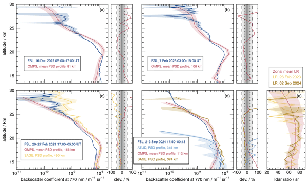
Figure 5 shows comparisons of the FSL BSC and the BSC derived from satellite measurements on four separate days, along with the associated error bars. The error estimation of the lidar-derived BSC, which only considers the error of the photon count, is explained in Sect. 2.2.5. The procedure for estimating errors in the BSC derived from the three satellite products is described in Appendix B. Figures 5(a)–(d) show the FSL BSC averaged over several hours and averaged BSC profiles from collocated OMPS-LP measurements taken with a maximum spatial distance of 175 km and calculated with a mean zonal lidar ratio profile. The temporal difference of collocated measurements is less than one day for Figs. 5(a)–(c) and less than one and a half days for Fig. 5(d). The temporal and spatial requirements were chosen so that at least two collocations are available for each comparison made.

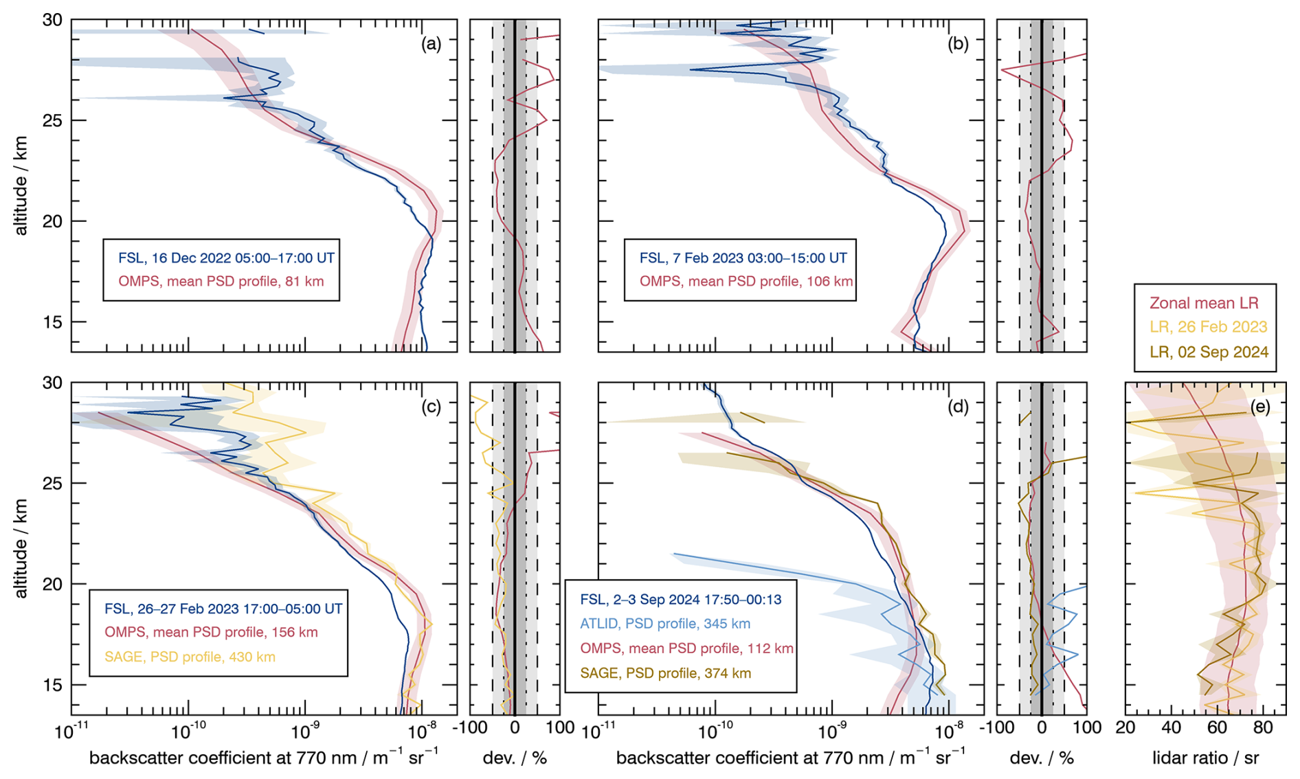
Figure 5 Comparison of the BSC from four FSL measurements (in dark blue) averaged over several hours with the derived BSC at 770 nm from collocated satellite measurements in (a)–(d). The mean spatial distance of these collocated measurements from Kühlungsborn is given. For OMPS-LP, the calculated BSC for a zonal lidar ratio profile averaged over the duration of the SAGE III/ISS mission (see Sect. 2.3) is shown in red. The SAGE III/ISS BSC calculated with a lidar ratio depending on the PSD of the measurement is shown in yellow. A mean ATLID BSC profile, converted to 770 nm, is shown in light blue. The percentage deviation of the FSL from the satellite measurements is shown on the right-hand side of each subplot. The range of a deviation of 50 % and 25 % is indicated by a dashed and dotted line, respectively. (e): Lidar ratios (LR) used, shown in the corresponding colours.

Figure 5(c) and (d) additionally show BSC profiles with lidar ratios profiles, derived from collocated SAGE III/ISS measurements and their associated PSD parameters, with a maximum spatial distance of 450 km and a temporal difference of less than one day in Fig. 5(c) and less than four days for Fig. 5(d). These requirements were chosen in order to have one collocated SAGE-III/ISS measurement at both times. During northern winter, SAGE III/ISS only covers the mid-latitudes to a limited extent, therefore no suitable collocated SAGE III/ISS measurements are available for December 2022 and early February 2023. The lidar ratios with corresponding errors are shown in Fig. 5(e).

ATLID measurements are available from July 2024 onwards, which means that a comparison is only possible for Fig. 5(d). Measurements with a maximum distance of 350 km from Kühlungsborn were averaged for the orbit 1510B, which took place during the FSL measurement. The wavelength conversion was performed using the same PSD profile as for SAGE III/ISS.

In 15–25 km altitude, the average absolute deviation between lidar and satellite is 25 %. At the peak of the stratospheric aerosol layer, the lidar BSC is 35 %–45 % smaller than the BSC derived from satellite measurements. Above an altitude of 26 km, the noise increases and the deviations tend to become larger.

The measurements compared are not perfect collocations, as the same air volumes are not measured. This is due to the temporal and spatial distance between the satellite measurements and the lidar measurements, which is expected to have an influence, especially in winter measurements due to the stronger atmospheric dynamics. As can be seen in Fig. 4, a deviation in the profiles is expected simply because of the temporal difference between the measurements. In addition, unlike lidar, the satellite measurements are not point measurements and the horizontal resolution is coarser.

The error of the BSC increases with altitude. This is least significant for the BSC shown from OMPS-LP measurements, as several measurements are averaged here and a zonal mean lidar ratio is used. The errors shown for the three different BSCs should be interpreted with caution, as they contain different error contributions depending on the instrument and are not equally representative of the total error, see Appendix B.

4 Discussion

The measurement depicted in Fig. 4 illustrates the vertical and temporal distribution of stratospheric aerosols, most notably the distinct Junge layer situated between 16 and 22 km. A pronounced decrease in backscatter above 22 km indicates the transition toward lower aerosol concentrations in the upper stratosphere. Above 26 km, the signal-to-noise ratio decreases significantly as a result of the lower abundance of sulphate aerosols, which limits the instrument's aerosol sensitivity at these altitudes. To facilitate future investigations of higher-altitude phenomena, such as MSPs, detection efficiency could be enhanced by increasing the backscattered signal through the integration of power scaled Alexandrite-lasers or larger telescope apertures. Furthermore, the implementation of narrower spectral bandwidths for both the laser and the detection filters could further improve sensitivity, although the current configuration already operates near the current performance limits.

From mid to late February 2023, there is significant small-scale variation in aerosol measurements using lidar and satellites over Kühlungsborn (not shown). This is due to the polar vortex shifting towards the mid-latitudes and moving horizontally. Consequently, the discrepancy between the satellite profiles of the two instruments in 17–25 km altitude is larger at the end of February 2023 than during the more quiescent late-summer period in September 2024. Because of the same reason, the spatial distance of the SAGE III/ISS collocation in February 2023 (over 400 km further south than FSL and OMPS-LP) has a greater influence than it does in September 2024. We expect improved comparison results once a larger sample of lidar measurements is available for comparison to satellite data, because then variability at small spatial and temporal scales will average out to a greater extent.

Comparison with satellite-derived backscatter demonstrates overall good agreement and highlights the complementary nature of the datasets. OMPS‑LP and SAGE III/ISS rely on spectrometer-based extinction retrievals. Although these satellites offer broad spatial coverage, their coarse vertical resolution and horizontal averaging reduce sensitivity to short-term and fine-scale variability. The high-resolution FSL measurements capture aerosol structures, such as the layering phenomena visible in Fig. 4, which cannot be resolved using common remote sensing methods. The observability of streamers and frozen-in anticyclones using aerosols as tracers has been demonstrated with satellite instruments (Löns et al., 2025), and FSL measurements offer the potential to observe even finer-scale structures vertically and temporally.

Deviations between the lidar measurements and satellite profiles, especially around 20 km, can be partly attributed to limited spatiotemporal collocation, horizontal smoothing in limb observations, and assumptions that must be made when converting the signal measured by the satellite into the extinction coefficient and BSC. Particularly in the atmosphere unaffected by the polar vortex in September 2024, the quality of spatiotemporal collocation is less important, as the stratospheric profiles in the vicinity of Kühlungsborn vary only slightly over time. Nevertheless, a comparison of lidar and satellite data at an altitude of 20–25 km shows that the signal in the lidar BSC is about 25% lower than in the satellite BSC. The backscatter measured with FSL is therefore lower than would be expected from the calculated backscatter derived from limb and solar occultation measurements. If the actual particle size distribution deviates from the assumed unimodal log-normal distribution for example, due to bimodality or increased coarse-mode fraction, systematic biases may occur, as the size range dominating the scattering signal exerts disproportionate influence (von Savigny and Hoffmann, 2020; Wrana et al., 2025). Dynamically active winter conditions can further amplify these discrepancies. Despite these limitations in the comparison of different observation methods, the high temporal and vertical resolution of the lidar ensures reliable detection and continuous monitoring of stratospheric aerosol structures, providing critical context for interpreting satellite observations.

5 Conclusions and Outlook

This study demonstrates that the FSL method allows for highly sensitive and high-resolution measurements of stratospheric aerosols, even under full daylight conditions. By determining both the BSR and the corresponding BSC, it becomes possible to monitor the dynamics of the Junge layer with a vertical and temporal accuracy that surpasses that achievable with the satellite datasets considered in this work.

High-resolution FSL profiles reveal pronounced vertical structures and rapid temporal variability within the stratospheric aerosol layer. Comparisons with aerosol products from OMPS-LP and SAGE III/ISS show generally good agreement, with an average absolute deviation of about 25 % between 15 and 25 km altitude. Remaining differences can largely be attributed to spatiotemporal mismatches between ground-based and satellite observations, the coarser vertical resolution and horizontal averaging inherent to satellite retrievals, and the assumptions required to derive backscatter-related quantities from limb-viewing measurements.

The stability of FSL retrievals demonstrates the suitability of the method for continuous monitoring under varying atmospheric conditions. In this context, FSL observations provide a valuable reference for the validation and interpretation of satellite aerosol products and allow capturing short-term dynamical variability that would otherwise remain unresolved.

Ongoing developments of the lidar system within the EULIAA project (European Lidar Array for Atmospheric Climate Monitoring) will further improve the sensitivity of FSL measurements through methodological advances, including higher laser power, narrower filters, and longer averaging times. This enables reliable observations even at very low aerosol concentrations and allows the FSL method to cover an increasingly larger range of particle sizes in the stratosphere also above the Junge layer. Here, a higher proportion of natural MSPs and artificial particles from re-entering satellites, as well as emitted particles from rocket engines, is to be expected. The additional use of depolarization measurements enables targeted distinction between spherical and non-spherical particles, allowing these sensitive signals to be captured accurately.

Appendix A: Table of lidar parameters

As the VAHCOLI system is continuously being developed, its performance and hardware are subject to ongoing improvements. Table A1 provides an overview of the principal specifications of the VAHCOLI configuration (version 1 and 2) employed for the measurements presented in this paper. Version 2 offers the possibility of taking measurements higher up in the atmosphere, due to its higher frequency and the resulting greater energy density. Full overlap between the receiver field of view and the laser beam is achieved above 20 km.

Table A1 VAHCOLI system specifications and parameters for version 1 and version 2.

Appendix B: Error estimation for the backscatter coefficient from satellite measurements

The error in the extinction coefficient depending on wavelength and height k_ext(z,λ) provided in the OMPS-LP data product consists only of the error in calculating Rayleigh scattering. The impact of an error in the assumed aerosol microphysical parameters for the extinction coefficient in OMPS-LP is not included. Firstly, the error of the Ångström exponent is calculated.

$$\begin{array}{}\text{(B1)}& \mathrm{\Delta }\mathit{\alpha }\left(z\right)={\displaystyle \frac{\mathrm{1}}{\ln ({\mathit{\lambda }}_{\mathrm{2}}/{\mathit{\lambda }}_{\mathrm{1}})}}\cdot \sqrt{{\left({\displaystyle \frac{\mathrm{\Delta }{k}_{\text{ext}}(z,{\mathit{\lambda }}_{\mathrm{1}})}{k_{\text{ext}}(z,{\mathit{\lambda }}_{\mathrm{1}})}}\right)}^{\mathrm{2}}+{\left({\displaystyle \frac{\mathrm{\Delta }{k}_{\text{ext}}(z,{\mathit{\lambda }}_{\mathrm{2}})}{k_{\text{ext}}(z,{\mathit{\lambda }}_{\mathrm{2}})}}\right)}^{\mathrm{2}}}\end{array}$$

Subsequently, the error contained in the data set is interpolated using the Ångström exponent for the extinction coefficient at a wavelength of 770 nm.

$$\begin{array}{}\text{(B2)}& \begin{array}{rl}\mathrm{\Delta }{k}_{\text{ext}}(z,{\mathit{\lambda }}_{\text{lidar}})& =\sqrt{{\left({\left({\displaystyle \frac{{\mathit{\lambda }}_{\text{lidar}}}{{\mathit{\lambda }}_{\mathrm{1}}}}\right)}^{-\mathit{\alpha }\left(z\right)}\cdot \mathrm{\Delta }{k}_{\text{ext}}(z,{\mathit{\lambda }}_{\mathrm{1}})\right)}^{\mathrm{2}}}\\ & +{\left(k_{\text{ext}}(z,{\mathit{\lambda }}_{\text{lidar}})\cdot \ln \left({\displaystyle \frac{{\mathit{\lambda }}_{\text{lidar}}}{{\mathit{\lambda }}_{\mathrm{1}}}}\right)\cdot \mathrm{\Delta }\mathit{\alpha }\left(z\right)\right)}^{\mathrm{2}}\end{array}\end{array}$$

Finally, the error of the extinction coefficient and the standard deviation of the zonal mean lidar ratio profile at each altitude step ΔΛ(z), as determined in Sect. 2.3, are propagated via error propagation.

$$\begin{array}{}\text{(B3)}& \mathrm{\Delta }{\mathit{\beta }}_{\text{Aer}}\left(z\right)={\mathit{\beta }}_{\text{Aer}}\left(z\right)\cdot \sqrt{{\left({\displaystyle \frac{\mathrm{\Delta }{k}_{\text{ext}}\left(z\right)}{k_{\text{ext}}\left(z\right)}}\right)}^{\mathrm{2}}+{\left({\displaystyle \frac{\mathrm{\Delta }\mathrm{\Lambda }\left(z\right)}{\mathrm{\Lambda }\left(z\right)}}\right)}^{\mathrm{2}}}\end{array}$$

The error of the BSC for SAGE III/ISS calculated with a single lidar ratio profile is also shown in Fig. 5. It is important to note that the use of the derived PSD parameters contained in the SAGE III/ISS data products of the statistical median of median radius r_med, geometric standard deviation σ_g and number density N₀ as a combination does not provide an accurate representation of the original measurement, as each parameter is only a weighted statistic. Mie calculations using this combination do not reproduce the originally measured spectrum. In addition, the derived PSD parameters contained in the SAGE III/ISS data products use refractive indices for stratospheric aerosols that are not temperature-corrected. This is expected to cause a bias, particularly in the retrieval of number density. Moreover, the calculation of the number density in V6 of SAGE III/ISS contains a further bias. According to the procedure in Knepp et al. (2024), the extinction coefficient at 1020 nm is first calculated for each combination of median radius and geometric standard deviation in the solution space with a number density of 1 cm⁻³. The number density is then formed via the ratio to the extinction coefficient at 1020 nm. This introduces a bias, as the ratio is always formed to the central position in the solution space and not to the actual position, which can range from k₁₀₂₀−σ₁₀₂₀ to k₁₀₂₀+σ₁₀₂₀.

To reduce the influence of these error contributions, the PSD parameters are only used to simulate the lidar ratio from the combination of median radius and geometric standard deviation for a wavelength of 770 nm using the Mie code. The extinction coefficient at 770 nm and its error, on the other hand, are calculated for the SAGE III/ISS measurements using the Ångström exponent. Error propagation for calculation of the lidar ratio can be performed using the statistical data of the PSD parameters. The standard deviations u_x of the median radius and geometric standard deviation can roughly be calculated from the statistical data obtained in the data set for the weighted median absolute deviations (MAD) within the solution space, assuming a normal distribution (Leys et al., 2013).

$$\begin{array}{}\text{(B4)}& u_x\left(z\right)={\text{MAD}}_x\left(z\right)\cdot \mathrm{1.4826}\end{array}$$

The standard deviations u_x can be used to calculate the partial derivative of the lidar ratio at height z for a variation of each parameter x by ±1 standard deviation, with x being the median radius or the geometric standard deviation.

$$\begin{array}{}\text{(B5)}& {\displaystyle \frac{\partial \mathrm{\Lambda }\left(z\right)}{\partial x\left(z\right)}}\approx {\displaystyle \frac{\mathrm{\Lambda }\left(x\right(z)+u_x(z\left)\right)-\mathrm{\Lambda }\left(x\right(z)-u_x(z\left)\right)}{\mathrm{2}\cdot u_x\left(z\right)}}\end{array}$$

Neglecting the covariances, the error of the lidar ratio can now be calculated as the sum of the error contributions of the median radius and geometric standard deviation to the lidar ratio, which are assumed to be independent.

$$\begin{array}{}\text{(B6)}& \mathrm{\Delta }\mathrm{\Lambda }\left(z\right)=\sqrt{{\left({\displaystyle \frac{\partial \mathrm{\Lambda }\left(z\right)}{\partial r_{\text{med}}\left(z\right)}}\cdot u_{r_{\text{med}}}\left(z\right)\right)}^{\mathrm{2}}+{\left({\displaystyle \frac{\partial \mathrm{\Lambda }\left(z\right)}{\partial {\mathit{\sigma }}_g\left(z\right)}}\cdot u_{{\mathit{\sigma }}_g}\left(z\right)\right)}^{\mathrm{2}}}\end{array}$$

As in Eq. (B3), the total error of the BSC can now be determined from the error of the extinction coefficient at 770 nm and the error of the lidar ratio. For ATLID, the error of the BSC at 770 nm can be determined in the same way as in Eqs. (B5), (B6) and (B3). However, instead of LR, the ratio of the backscattering cross sections at 770 and 355 nm is used for this.