Polarization calibration of spaceborne lidar using dense cirrus–scattered solar background with molecular scattering correction

Accurate calibration is essential for spaceborne polarization-sensitive lidars, as biases in depolarization ratio measurements can significantly affect the retrieval of cloud and aerosol properties. A polarization calibration technique based on solar background signals scattered by optically thick ice clouds (OTIC) provides a semi-continuous daytime calibration capability that complements onboard pseudo-depolarizer (PD) methods. This method was successfully applied to data from the Cloud-Aerosol Transport System (CATS) lidar at 1064 nm, where molecular scattering effects are negligible. However, at shorter wavelengths, molecular scattering of sunlight between the lidar and the OTIC layer polarizes the background signal and introduces systematic biases. We present a molecular scattering correction (MSC) scheme based on vector radiative transfer modeling (VRTM) to account for this effect and demonstrate its performance using observations from the Cloud-Aerosol Lidar with Orthogonal Polarization (CALIOP). The results show that molecular scattering introduces a daytime bias of approximately 1 % at 532 nm, which is effectively removed by the VRTM-based MSC, yielding close agreement with onboard PD calibrations. For the Earth Cloud, Aerosol and Radiation Explorer (EarthCARE) Atmospheric Lidar (ATLID) operating at 355 nm, model calculations indicate that molecular scattering contributions can be more than five times larger than at 532 nm, underscoring the necessity of applying an MSC when the OTIC calibration technique is employed. Together, these results establish the OTIC calibration technique, combined with MSC, as a robust approach for achieving accurate polarization calibration across current and future spaceborne lidar missions.

1 Introduction

The depolarization ratio, the ratio of signal components polarized perpendicular and parallel to the laser's linear polarization plane, is a key parameter for identifying atmospheric particles. It has been widely used to distinguish ice crystals from water droplets (Pal and Carswell, 1973; Sassen, 1991), to separate irregularly shaped mineral aerosols from spherical aerosol types (Murayama et al., 1999; Liu et al., 2002), and to quantify multiple scattering in water clouds (Hu et al., 2001, 2007).

Accurate polarization calibration is therefore essential for the reliable interpretation of depolarization measurements. Without proper calibration, systematic biases in the depolarization ratio can lead to misclassification of particle types and errors in retrieved optical properties (e.g., Sassen and Zhu, 2009). This requirement is particularly critical for spaceborne polarization-sensitive lidar systems, in which the depolarization ratio plays a central role in data processing and particle typing, as demonstrated for the Cloud-Aerosol Lidar with Orthogonal Polarization (CALIOP) onboard the Cloud-Aerosol Lidar and Infrared Pathfinder Satellite Observations (CALIPSO) mission (Winker et al., 2009; Omar et al., 2009; Hu et al., 2009; Liu et al., 2009).

A critically important component of any polarization calibration is the determination of the relative gain between the parallel and perpendicular detection channels, commonly expressed as the polarization gain ratio (PGR). In CALIOP, this was accomplished using an onboard pseudo-depolarizer (PD) that, when inserted into the receiver's optical path, completely depolarized the incident backscattered signal and thus provided a nonpolarized light source, independent of the incident polarization state. With sufficient data averaging, this method enabled accurate PGR determination and ensured long-term calibration stability (Hunt et al., 2009; Powell et al., 2009).

However, this approach cannot provide continuous polarization calibration, because insertion of the PD switches the data acquisition mode from routine science measurements to calibration mode, thereby interrupting continuous data collection. A typical CALIOP nighttime PGR calibration required approximately 32 min, while daytime PGR calibrations interrupted science measurements for 3–5 d. Reducing both the duration and frequency of these interruptions remains a challenge, motivating the development of techniques that enable continuous or near-continuous polarization calibration.

To address this limitation, Liu et al. (2004) proposed an alternative daytime calibration technique based on the observation that sunlight scattered by optically thick ice clouds (OTICs) becomes effectively unpolarized due to internal reflections and multiple scattering among irregular ice particles. This naturally depolarized signal provides a stable reference for lidar polarization calibration. A major advantage of this method is that it enables semi-continuous monitoring of daytime polarization calibration without interrupting science observations. The technique was developed and validated using airborne Cloud Physics Lidar (CPL) measurements at 1064 nm (Liu et al., 2004) and subsequently adopted for 1064 nm polarization calibration on the spaceborne Cloud-Aerosol Transport System (CATS) (Pauly et al., 2019).

While the OTIC method is highly effective at 1064 nm, its application at shorter wavelengths, such as CALIOP's 532 nm or the Earth Cloud, Aerosol and Radiation Explorer (EarthCARE) Atmospheric Lidar (ATLID) at 355 nm (Wehr et al., 2023), requires an additional correction for molecular scattering contributions to the total background signals. The magnitude of molecular scattering between the lidar and the OTIC cloud-top altitude scales with wavelength approximately as λ⁻⁴. Because molecular scattering of sunlight is highly polarized, at shorter wavelengths it can introduce spectrally dependent residual polarization that, if not properly corrected, will bias subsequent PGR estimates.

In this paper, we present the theoretical foundation of a molecular scattering correction (MSC) method for improved PGR determination. We further demonstrate its effectiveness using solar background signals from OTIC detected in CALIOP measurements.

2 Theoretical Basis

Figure 1 presents geometry of space lidar observations. The scattering powers for single scattering of sunlight by a single particle are given by (Bohren and Huffman, 1983; Hu et al., 2001; Liu et al., 2004):

$$\begin{array}{}\text{(1)}& \begin{array}{r}{P}_{⟂}={\displaystyle \frac{\mathrm{1}}{\mathrm{2}}}{\mathit{\sigma }}_{\text{sca}}{I}_{\mathrm{0}}\left(P_{\mathrm{11}}\right(\mathrm{\Theta })+P_{\mathrm{12}}(\mathrm{\Theta }\left)\cos \right(\mathrm{2}\mathrm{\Delta }\mathit{\varphi }\left)\right)\\ P_{\parallel }={\displaystyle \frac{\mathrm{1}}{\mathrm{2}}}{\mathit{\sigma }}_{\text{sca}}{I}_{\mathrm{0}}\left(P_{\mathrm{11}}\right(\mathrm{\Theta })-P_{\mathrm{12}}(\mathrm{\Theta }\left)\cos \right(\mathrm{2}\mathrm{\Delta }\mathit{\varphi }\left)\right)\end{array}\end{array}$$

where, I₀ is the intensity of the incident light, while P_⟂ and P_∥ represent, respectively, the perpendicular and parallel components of the scattered light with respect to the scattering plane, defined by the incident sunlight and the lidar viewing direction, and the subscripts ⟂ and ∥ represent perpendicular and parallel components throughout the paper, respectively. σ_sca is the scattering cross section of the cloud particles and P₁₁ and P₁₂ are elements of the scattering phase matrix. The scattering angle Θ is defined as the angle between the incident sunlight and the upwelling sunlight along the lidar's viewing direction (i.e., the angle formed by the two orange lines in Fig. 1). Δϕ is the relative angle between (1) the scattering plane, and (2) the plane defined by the polarization direction of the lidar's parallel channel (perpendicular to the orbital track in the case of CALIOP) and the lidar viewing direction.

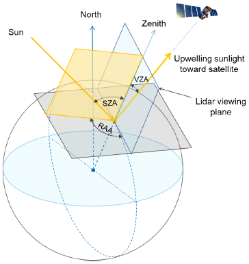
Figure 1 Geometry of lidar observations. SZA denotes the solar zenith angle, VZA is the lidar's viewing zenith angle, and RAA is the relative azimuth angle between the sunlight propagation plane and the lidar viewing plane. In the case of CALIOP, the viewing plane coincides with the orbiting plane, and the polarization direction of the laser is perpendicular to the lidar viewing plane.

Numerical calculations (e.g., Hu et al., 2001; Liu et al., 2004) show that the parallel and perpendicular components of scattered sunlight are nearly equal for cirrus clouds, due to multiple internal reflections within their irregular ice crystals. Moreover, external multiple scattering among particles can further depolarize the scattered sunlight. This effect becomes more significant in spaceborne lidar observations, such as those from CALIOP, due to the large footprint of their field-of-view (Hu et al., 2007). A larger receiver footprint collects more higher-order multiple-scattered photons, which tend to increasingly scramble the polarization state and thereby depolarize the detected signal.

For Rayleigh scattering (molecular scattering), the first two elements of the phase matrix are $P_{\mathrm{11}}\left(\mathrm{\Theta }\right)=\frac{\mathrm{3}}{\mathrm{4}}(\mathrm{1}+{\cos }^{\mathrm{2}}(\mathrm{\Theta }\left)\right)$ and $P_{\mathrm{12}}\left(\mathrm{\Theta }\right)=-\frac{\mathrm{3}}{\mathrm{4}}{\sin }^{\mathrm{2}}\left(\mathrm{\Theta }\right)$ (Yang and Liou, 1998; Zhai et al., 2009). Substituting these elements into Eq. (1), the two polarization components for molecular scattering, perpendicular and parallel to the scattering plane, are derived as follows:

$$\begin{array}{}\text{(2)}& \begin{array}{rl}& P_{⟂}={\displaystyle \frac{\mathrm{3}}{\mathrm{8}}}{\mathit{\sigma }}_{\text{sca}}{I}_{\mathrm{0}}\left(\right(\mathrm{1}+{\cos }^{\mathrm{2}}\left(\mathrm{\Theta }\right))-{\sin }^{\mathrm{2}}(\mathrm{\Theta }\left)\cos \right(\mathrm{2}\mathrm{\Delta }\mathit{\varphi }\left)\right)\\ & P_{\parallel }={\displaystyle \frac{\mathrm{3}}{\mathrm{8}}}{\mathit{\sigma }}_{\text{sca}}{I}_{\mathrm{0}}\left(\right(\mathrm{1}+{\cos }^{\mathrm{2}}\left(\mathrm{\Theta }\right))+{\sin }^{\mathrm{2}}(\mathrm{\Theta }\left)\cos \right(\mathrm{2}\mathrm{\Delta }\mathit{\varphi }\left)\right)\end{array}\end{array}$$

The molecular scattering cross section can be expressed as (Bodhaine et al., 1999):

$$\begin{array}{}\text{(3)}& {\mathit{\sigma }}_{\text{sca}}={\displaystyle \frac{\mathrm{24}{\mathit{\pi }}^{\mathrm{3}}}{{\mathit{\lambda }}^{\mathrm{4}}{N}^{\mathrm{2}}}}{\left({\displaystyle \frac{n^{\mathrm{2}}-\mathrm{1}}{n^{\mathrm{2}}+\mathrm{2}}}\right)}^{\mathrm{2}}F\end{array}$$

where λ is the wavelength, N is the molecular number density, n is the refractive index of air, and F is the King correction factor.

Molecular scattering of sunlight is strongly polarized, with the degree of polarization determined by the relative orientation of the scattering plane and the lidar's parallel polarization plane (the plane defined by the laser polarization direction and the line of sight). When using solar background signals from OTIC to derive the PGR, accounting for molecular scattering contributions to the background signals is essential, as they can introduce residual polarized signals that would bias the derivation. At 1064 nm, molecular scattering is very weak and can be safely ignored. However, because the scattering cross section scales with wavelength as λ⁻⁴ (Eq. 3), relative to 1064 nm, the molecular scattering contribution is ∼16 times larger at 532 nm and ∼81 times larger at 355 nm. These large differences make it essential to correct space-based PGR estimates for molecular scattering at shorter wavelengths.

In Appendix A we present mathematical derivations of two different approaches that can be used to calibrate the PGR. The first uses the ratio of the directly measured mean background signals (e.g., as in Liu et al., 2004) while the second uses the ratio of the root-mean-squares (RMS) of the background signals. Because identical results are obtained using either method, data availability will dictate the choice of technique to apply. The following discussions leverage the mathematical derivations given in Appendix A to further explore both approaches.

Replacing the expression for digitizer counts measured in the perpendicular and parallel channels of the lidar receiver (i.e., $N_{\text{dc},⟂}$ and $N_{\text{dc},\parallel }$ in Eq. A5) with BKG_⟂ and BKG_∥, the equation for deriving PGR from OTIC background measurements at long wavelengths becomes,

$$\begin{array}{}\text{(4)}& \text{PGR}={\displaystyle \frac{{\stackrel{\mathrm{‾}}{\text{BKG}}}_{⟂}}{{\stackrel{\mathrm{‾}}{\text{BKG}}}_{\parallel }}},\end{array}$$

where $\stackrel{\mathrm{‾}}{\text{BKG}}$ denotes the mean background signals, and the subscripts ⟂ and ∥ represent perpendicular and parallel channels, respectively.

Adapting this formulation for shorter wavelengths with MSC is straightforward:

$$\begin{array}{}\text{(5)}& \text{PGR}={\displaystyle \frac{\stackrel{\mathrm{‾}}{{\text{BKG}}_{\mathrm{t},⟂}}-\stackrel{\mathrm{‾}}{{\text{BKG}}_{\mathrm{m},⟂}}}{\stackrel{\mathrm{‾}}{{\text{BKG}}_{\mathrm{t},\parallel }}-\stackrel{\mathrm{‾}}{{\text{BKG}}_{\mathrm{m},\parallel }}}}.\end{array}$$

where the subscripts t and m denote the total background signal measured (i.e., contributions from molecules and OTIC) and the molecular-only component modeled, respectively. Equation (5) is the primary form for use in the OTIC technique.

For CALIOP, ready implementation of Eq. (5) is complicated by the receiver's background subtraction architecture. As explained in detail in Hunt et al. (2009), CALIOP's 532 nm parallel and perpendicular channel background magnitudes are separately measured by dedicated background monitors at single shot resolution at high altitudes (97–112 km) where no detectable atmospheric lidar backscatter occurs. To prevent overflows in the downstream science digitizers, these background signals were removed from each profile using an onboard electronic feedback circuit. Within this feedback circuit, signal levels were recorded using stand-alone 14-bit digitizers that were wholly separate from the science digitizers subsequently used to sample the background-subtracted lidar backscatter profiles. Random noise in the background signals was measured using the science digitizers at altitudes of 65–80 km (reported as the parallel and perpendicular “RMS baseline” parameters in the CALIOP Level 1 data products), where atmospheric lidar backscatter is also largely negligible. Both the background monitor magnitudes and the random noise estimates are downlinked in the science data stream. In the early stages of the CALIOP instrument development, RMS baseline values were called out as a key measurement required for accurate layer detection (Vaughan et al., 2009). In the following years, the RMS baseline numbers proved critical in the development of several other essential calibration and science retrieval algorithms (e.g., Hostetler et al., 2006; Powell et al., 2009; Lu et al., 2018).

Therefore, the PGR derived using Eq. (5) would represent the gain ratio of the background monitor signal acquisition circuits rather than the required gain ratio of the science data acquisition circuits needed in CALIOP data processing. Consequently, in the following section we develop an RMS-based technique to derive the required PGR for lidar systems such as CALIOP that do not directly measure background signal levels using the science data acquisition circuit. The PGR equation based on the background RMS noise, including MSC, can be derived from Eq. (A8) in Appendix A as

$$\begin{array}{}\text{(6)}& \text{PGR}={\left({\displaystyle \frac{F_{\mathrm{m},\parallel }}{F_{\mathrm{m},⟂}}}\right)}^{\frac{\mathrm{1}}{\mathrm{2}}}{\left({\displaystyle \frac{{\text{RMS}}_{\text{OTIC},⟂}^{\mathrm{2}}-{\text{BDR}}_{⟂}{K}_{\mathrm{0},⟂}{I}_{\mathrm{0}}}{{\text{RMS}}_{\text{OTIC},\parallel }^{\mathrm{2}}-{\text{BDR}}_{\parallel }{K}_{\mathrm{0},\parallel }{I}_{\mathrm{0}}}}\right)}^{\frac{\mathrm{1}}{\mathrm{2}}}\end{array}$$

where F_m is the excess noise factor introduced to correct detector multiplication noise contained in the measured background noise RMS. Unlike the BKG-based PGR determination using Eq. (5) that is a simple ratio of background signals with MSC, application of Eq. (6) requires additional knowledge of the ratio $F_{\mathrm{m},\parallel }/F_{\mathrm{m},⟂}$. Because identical PMTs are used in the parallel and perpendicular channels, this ratio is expected to be close to unity; therefore, in this paper, we assume $F_{\mathrm{m},\parallel }/F_{\mathrm{m},⟂}=\mathrm{1}$. The ${\text{BDR}}_{⟂}{K}_{\mathrm{0},⟂}{I}_{\mathrm{0}}$ and ${\text{BDR}}_{\parallel }{K}_{\mathrm{0},\parallel }{I}_{\mathrm{0}}$ terms in Eq. (6) represent the modeled molecular scattering contributions to the observed backscattered solar variance for the lidar perpendicular and parallel channel, respectively, with

$$\begin{array}{}\text{(7)}& {\displaystyle }{\mathrm{\text{BDR}}}_{\parallel }={\displaystyle \frac{\left({\text{BDR}}_I+{\text{BDR}}_Q\right)}{\mathrm{2}}},{\text{BDR}}_{⟂}={\displaystyle \frac{\left({\text{BDR}}_I-{\text{BDR}}_Q\right)}{\mathrm{2}}}\text{(8)}& {\displaystyle }{I}_{\mathrm{0}}={\displaystyle \frac{\mathrm{1}}{\mathit{\pi }}}{D}_{\mathrm{0}}\cos \left(\text{SZA}\right)S_{\mathrm{0}}\end{array}$$

where BDR is the bidirectional reflectance, which describes how the atmosphere–surface system reflects incoming light as a function of both the illumination and viewing geometries. In the molecular scattering correction presented here, only the contribution from atmospheric molecular scattering is considered. The quantities BDR_I and BDR_Q are derived from the Stokes parameters (I) and (Q), which represent the intensity and linear polarization components of the scattered light, respectively. These Stokes parameters are calculated for molecular scattering using a polarization-sensitive vector radiative transfer model (VRTM, Zhai et al., 2009 We note that, whereas Eq. (2) describes the scattering of incident light by a single particle, the BDR terms used in Eq. (7) characterize the emergent radiation field of the atmosphere–surface system after radiative transfer, in which extinction, multiple scattering, and polarization are taken into account. Consequently, the bidirectional reflectance varies with both the solar illumination and sensor viewing geometries.

S₀ is the solar constant at the lidar wavelength, and D₀ is Earth–Sun distance correction factor given by Iqbal (1983)

$$\begin{array}{}\text{(9)}& \begin{array}{rl}{D}_{\mathrm{0}}=& \mathrm{1.00011}+\mathrm{0.034221}\times \cos \left(\mathit{\phi }\right)+\mathrm{0.00128}\times \sin \left(\mathit{\phi }\right)\\ & +\mathrm{0.000719}\times \cos \left(\mathrm{2}\mathit{\phi }\right)+\mathrm{0.000077}\times \sin \left(\mathrm{2}\mathit{\phi }\right)\end{array}\end{array}$$

where

$$\begin{array}{}\text{(10)}& \mathit{\phi }={\displaystyle \frac{\mathrm{2}\mathit{\pi }(d-\mathrm{1})}{\mathrm{365}}}\end{array}$$

with d being the fractional day of the year. The scaling factors $K_{\mathrm{0},\parallel }$ and $K_{\mathrm{0},⟂}$ convert the magnitude and units of the modeled solar radiance into the measured solar background variance at the receiver digitizer. These coefficients can be determined empirically by comparing, for example, CALIPSO wide field-of-view camera (WFC) observations of bidirectional radiance of selected clouds with exactly collocated CALIOP measurements of the same clouds (Pitts et al., 2007). Because these conversion coefficients may vary over time and are generally expected to increase as the lidar system sensitivity degrades, periodic re-evaluation is likely necessary for a long-duration mission. Our sensitivity analysis shows that a 1 % change in these conversion coefficients results in a change of approximately 0.000061 in the derived PGR. Therefore, the PGR is not highly sensitive to uncertainties in the conversion coefficients at 532 nm. However, the sensitivity would increase rapidly at shorter wavelengths, since the molecular scattering scales as λ⁻⁴.

When the optical signals incident on both the parallel and perpendicular channels are equal, PGR estimates can be derived directly using Eq. (6). OTIC can therefore provide an effective light source for PGR estimation, provided that the molecular scattering contribution can be quantified and removed. To accomplish this, we use the VRTM developed by Zhai et al. (2009) to generate a lookup table (LUT) of the polarization components of the bidirectional reflectance (BDR) between the laser and cloud top for a fixed set of different cloud top altitudes. These BDR calculations are parameterized by solar zenith angle (SZA), lidar viewing zenith angle (VZA), and the relative azimuth angle (RAA) between the sunlight incident plane and the lidar viewing plane (see Fig. 1).

We note that, while the BDR components in the molecular scattering LUT are modeled with respect to the lidar viewing plane, the BDR components in Eq. (6) are defined with respect to the lidar parallel polarization plane. These two coordinate systems are not necessarily aligned. Therefore, a coordinate transformation is generally required to derive the BDR components in Eq. (6) from the modeled LUT. In the case of CALIOP, the laser polarization direction is perpendicular to the lidar viewing plane.

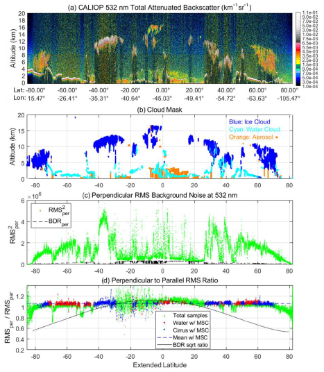
Figure 2 CALIOP measurements on 4 March 2013, beginning at 16:17:38 UTC. (a) Attenuated backscatter coefficients at 532 nm; (b) CALIOP feature mask for 5 km columns: blue, ice clouds; cyan, water clouds; orange, aerosols. (c) Squared RMS baseline signals (i.e., background noise) in the perpendicular channel (green dots), expressed in squared science digitizer counts. The black line shows the modeled molecular scattering contribution integrated from the topmost layer to the lidar, computed using a VRTM (Zhai et al., 2009). (d) Perpendicular-to-parallel RMS baseline signal ratio for all 5 km columns (green dots), OTIC PGR retrievals (blue dots) and PGR estimates retrieved by applying Eq. (5) to dense water clouds (red dots). The black line represents the square root of the perpendicular-to-parallel ratio of the BDR polarization components integrated from the surface to the top of the atmosphere.

Figure 2 shows an example of daytime CALIOP measurements. Panel (a) shows the 532 nm attenuated backscatter. The feature mask in panel (b) identifies ice clouds in blue, water clouds in cyan, and aerosols in orange. Panel (c) shows the corresponding squared RMS baseline signals (in green) measured in the perpendicular channel and the modeled molecular scattering contributions accumulated between the lidar and the OTIC top altitude (in black), calculated with the VRTM (Zhai et al., 2009). The comparison indicates that, at 532 nm, molecular scattering can represent a substantial fraction of the squared RMS background signal. This contribution increases when the feature top is lower and/or at higher latitudes where the solar elevation angle is smaller, due to the longer atmospheric path of sunlight. The mean fraction of molecular scattering contribution to the squared RMS is 0.17 with a standard deviation of 0.24 for all 5 km data points and reduces to 0.023 with a standard deviation of 0.011 for the cirrus samples selected (blue dots in Fig. 2d).

In Fig. 2d, the green dots show the perpendicular-to-parallel RMS ratio – i.e., the uncalibrated ratio of the RMS baseline signals – for each 5 km column in Fig. 2a. Blue dots show the PGRs retrieved using Eq. (6) in 5 km columns containing OTIC with RMS${}_{\parallel }>\mathrm{1000}$. Similarly, red dots show the PGRs retrieved using Eq. (6) in 5 km columns containing optically thick water clouds. Interestingly, the RMS ratios in these columns are very similar to those in the OTIC columns, largely due to increased multiple scattering within the water clouds, which depolarizes and randomizes the polarization state of sunlight. Dense water clouds could therefore also serve as suitable targets for PGR determination, provided that MSCs are applied and no overlying layers interfere with the measurement. For reference, the black line shows the square root of the perpendicular-to-parallel ratio of the BDR polarization components, equivalent to the molecular scattering depolarization ratio scaled by the squared PGR, calculated between the Earth's surface and the lidar. The observed RMS ratios closely match the scaled BDR polarization ratio in regions where molecular scattering dominates (e.g., around 50° S; see also Fig. 3).

To further evaluate the BDR calculation derived from the LUT, Fig. 3 presents one day of CALIOP measurements acquired on 4 March 2013. The data include 14 daytime granules, one of which is the granule shown in Fig. 2. Figure 3 displays the uncalibrated RMS baseline signal ratios (in green), the OTIC PGR measurements (in blue), and the square root of the scaled BDR depolarization ratio (black line). The upper bound (mainly in the tropics) and lower bound (at high latitudes) of the green dots correspond to 5 km columns where molecular scattering dominates, primarily over dark surfaces. The theoretical BDR depolarization ratio closely follows these molecular-dominated measurements, confirming the validity of the theoretical calculation.

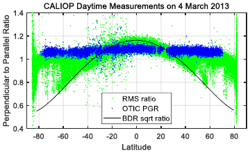
Figure 3 One day of CALIOP observations acquired on 4 March 2013, comprising a total of 14 daytime granules, one of which is the granule shown in Fig. 2. The green dots represent the RMS ratio, the blue dots denote the OTIC PGR, and the solid dark curve shows the square root of the scaled molecular-scattering BDR depolarization ratio at the surface. The theoretical BDR curve follows the upper (in the tropics) and lower (high latitudes) envelopes of the RMS ratios where molecular scattering dominates.

3 Application to Space Lidar Measurements

3.1 CALIOP Measurements

The proposed scheme was implemented in the CALIOP data processing system, beginning with the version 4.5 release, enabling near-continuous daytime calibration since cirrus clouds are almost always present globally. An overview of the calibration algorithm and an analysis of its performance are given in Vaughan et al. (2023). For the first decade of the mission, PD PGR calibrations were carried out only during nighttime orbits, under the assumption that the relative gain of the two receiver channels remained stable throughout the daytime portions of the orbits. Onboard PD PGR calibrations were performed once every few months within the span of a single orbit (Hunt et al., 2009; Powell et al., 2009), and the nighttime PGR values were applied to both daytime and nighttime data.

Beginning in November 2016, CALIPSO introduced “extended time” (ET) PGR calibration measurements, during which the PD was inserted continuously for 3–5 d. These ETs ensured that, with sufficient averaging, the calibration SNR measured during the daytime was comparable to the SNR achieved in previous nighttime only PD calibrations. The PGR is determined from the perpendicular-to-parallel ratio of the mean atmospheric lidar backscatter signals between 8.2 and 20.2 km altitude acquired during ET measurements. Before computing ratios, all signals are background subtracted, range squared corrected, and normalized with respect to laser energy and known electronic gains. Between November 2016 and January 2023, CALIPSO conducted ET PGR measurements on seven different occasions. To evaluate the MSC scheme, Fig. 4 compares the daily mean OTIC PGRs calculated during nominal science operations, both with (blue circles) and without (red circles) the molecular scattering corrections introduced in Eq. (6). Due to the inclusion of molecular scattering, the uncorrected OTIC PGRs are biased systematically low (by ∼1 %) relative to the corrected OTIC PGRs. Also shown in yellow diamonds are PGRs derived from an ET PD PGR calibration conducted during 22–25 November 2016. During these ET measurements, the PD completely depolarizes all incoming light, thus illuminating the detectors in both polarization channels with equal optical intensities. The PGRs derived from these measurements can therefore be considered as objective and unbiased (albeit noisy) truth. The OTIC PGRs calculated during the ET (green circles) are seen to be in excellent correspondence with the yellow diamonds, thus demonstrating the effectiveness of the molecular correction scheme.

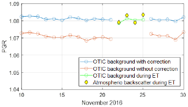
Figure 4 Daily mean OTIC PGR without (red) and with (blue) MSC using Eq. (6). The onboard PGR calibration using the PD was conducted over 22–25 November 2016 (green). Yellow diamonds show the corresponding daily mean PGRs derived from atmospheric backscatter signals within 8.2–20.2 km in the OTIC columns during the ET with the PD inserted.

Figure 5 shows global maps of the OTIC PGR derived from one month (January 2008) of CALIOP measurements, without (a) and with (b) MSC. Without MSC, the RMS ratio in Fig. 5a exhibits a pronounced latitudinal dependence, primarily caused by polarization of molecular scattering, which is sensitive to the solar elevation angle. After applying the MSC, this latitudinal dependence is largely removed, as shown in Fig. 5b. In the polar regions, some residual latitudinal dependence remains, likely due to the combined effects of decreased solar background strength and thermal effects associated with transitions between day and night.

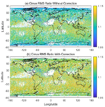
Figure 5 Global map of PGR (a) without and (b) with MSC from one month (January) of the CALIOP measurement year in 2008.

3.2 Applications to other space lidar measurements

The OTIC PGR calibration technique was successfully applied to the 1064 nm channel of the CATS lidar (Yorks et al., 2016). CATS, which operated on the International Space Station from 2015 to 2017, was designed to provide multi-wavelength backscatter and depolarization measurements to advance cloud and aerosol research and to demonstrate technologies for future spaceborne lidar missions. At 1064 nm, the contribution from molecular scattering is negligibly small, and therefore no MSC was applied.

The Aerosol and Carbon Detection Lidar (ACDL) aboard DQ-1 was successfully launched in April 2022. ACDL employs a high-spectral-resolution lidar (HSRL) technique (Dai et al., 2024) and provides global profiles of aerosol and cloud optical properties with high accuracy. The HSRL system measures the parallel and perpendicular components of total (Mie + Rayleigh) backscattering signal and Mie scattering filtered Rayleigh scattering signal at 532 nm. The OTIC technique could potentially be directly applied to determine the PGR for the two total polarization channels. However, doing so could be a challenging proposition, as ACDL does not make direct background measurements, but instead uses a novel algorithm to infer background magnitudes based on the atmospheric signals acquired in three different altitude regions (Meng et al., 2025).

EarthCARE, a joint mission of ESA and JAXA, was successfully launched in May 2024 (Wehr et al., 2023; Donovan et al., 2024). One of its primary instruments, ATLID, is a high-spectral-resolution lidar operating at 355 nm. ATLID provides vertically resolved measurements of aerosols and thin clouds, delivering profiles of backscatter, extinction, and depolarization with high sensitivity. Together with EarthCARE's other instruments – the Cloud Profiling Radar (CPR), the Multi-Spectral Imager (MSI), and the Broad-Band Radiometer (BBR)–ATLID observations will advance understanding of aerosol–cloud–radiation interactions and their role in the Earth's climate system. Unlike ACDL, ATLID measures the total perpendicular component and separates the total parallel component into Mie and Rayleigh channels. The Mie channel still contains a small fraction of Rayleigh (molecular) scattering. The OTIC calibration approach could be applied to its polarization calibration, in combination with a separate calibration of the Mie and Rayleigh channels.

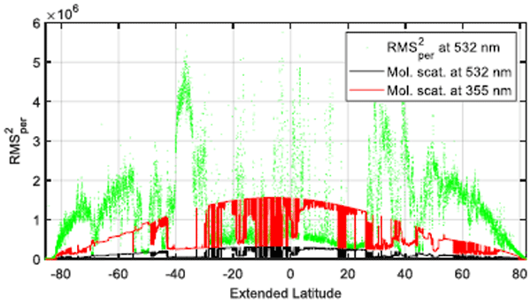
Figure 6 shows the squared RMS signal measured by CALIOP for the same orbit as in Fig. 2, together with the modeled molecular-scattering contribution to the squared RMS at 532 nm and the corresponding contribution expected if the lidar operated at the EarthCARE ATLID wavelength of 355 nm, simulated using the same VRTM (Zhai et al., 2009). The average ratio of molecular-scattering contributions between the two wavelengths is approximately 5.52 for the selected cirrus clouds. These results demonstrate that molecular scattering plays an even more significant role at 355 nm than at 532 nm and hence must be explicitly corrected when applying the OTIC calibration technique to EarthCARE lidar measurements.

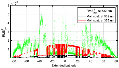
Figure 6 Squared RMS signal measured by CALIOP at 532 nm (green) and the squared RMS of the modeled molecular scattering (black) as shown in Fig. 2b, together with the simulated molecular scattering (squared RMS value) at the EarthCARE lidar wavelength of 355 nm (blue).

4 Application to airborne measurements

The OTIC technique can also be applied to airborne polarization-sensitive backscatter lidar measurements, as demonstrated using the CPL observations (Liu et al., 2004). As in spaceborne lidar applications, a molecular scattering correction is required at shorter wavelengths to achieve more accurate polarization calibration. Although dense water clouds can also serve as suitable calibration targets for spaceborne lidars because of the significant multiple scattering among water droplets within the large lidar footprint, as illustrated in Fig. 2, they may not be appropriate calibration targets for airborne lidars. The much smaller footprint of an airborne lidar results in substantially weaker multiple scattering, making the depolarization produced by multiple scattering much less pronounced and, consequently, rendering dense water clouds less suitable as calibration targets.

5 Summary

The OTIC lidar polarization calibration technique was originally developed using airborne polarization-sensitive backscatter lidar measurements at 1064 nm (Liu et al., 2004). The method is based on the principle that solar background radiation scattered from optically thick ice clouds is highly unpolarized and can therefore serve as an ideal light source for lidar polarization calibration. The technique was successfully applied to the spaceborne CATS lidar to calibrate its polarization measurements at 1064 nm (Pauly et al., 2019).

However, when the OTIC technique is applied to lidar polarization measurements at shorter wavelengths, such as CALIOP at 532 nm, molecular scattering between the lidar and the dense cloud top can polarize some fraction of the scattered background signal from OTIC. This effect must be corrected to achieve more accurate calibration. To address this issue, we have developed an MSC technique based on a molecular-scattering LUT generated using a VRTM. The theoretical basis of the MSC is described in the paper.

For CALIOP, the method was implemented beginning with Version 4.5 processing to complement onboard PD-based PGR calibrations (Vaughan et al., 2023). The results showed that molecular scattering at 532 nm between the lidar and the cloud top introduces a systematic daytime bias of approximately 1 %, which can be corrected using the LUT derived from the VRTM.

The method can also theoretically be applied to ACDL/DQ-1 to calibrate its HSRL 532 nm polarization measurements. The main challenges are the limited sampling height (40.4 km) and photon folding for the second shot of each laser pulse pair. Looking ahead, EarthCARE's ATLID, operating at 355 nm, will require rigorous MSC, as calculations indicate that molecular-scattering contributions at 355 nm are more than five times larger than those at 532 nm. Collectively, these applications demonstrate the robustness of the OTIC-based PGR calibration technique across multiple missions, while underscoring the increasing importance of MSC at shorter wavelengths.

Appendix A

Following Liu et al. (2006), the digitizer counts measured in the lidar receiver can be expressed as

$$\begin{array}{}\text{(A1)}& N_{\text{dc}}=\mathrm{2}\mathit{\eta }eB{G}_{\mathrm{m}}{G}_{\mathrm{A}}{T}_{\mathrm{s}}{n}_{\mathrm{p}}=G_{\mathrm{s}}{n}_{\mathrm{p}}\end{array}$$

where η is the quantum efficiency of the detector, e is the electron charge, B is the bandwidth, G_m is the detector multiplication gain if a photomultiplier tube (PMT) or an avalanche photodetector (APD) is used, and G_A is the product of the various conversion, scaling, and electronic gain factors. G_s=2ηeBG_mG_AT_s is a system composite gain, T_s is the system throughput of the lidar receiver, and n_p is the number of photons received by the telescope.

The standard deviation, ΔN_dc, of the digitizer counts, corresponding to the RMS baseline measurement calculated over CALIOP's 65–80 km altitude range, can be expressed as

$$\begin{array}{}\text{(A2)}& \mathrm{\Delta }{N}_{\text{dc}}=G_{\mathrm{s}}\sqrt{F_{\mathrm{m}}}\mathrm{\Delta }{n}_{\mathrm{p}}\end{array}$$

where F_m is the excess noise factor introduced to account for the multiplication noise in PMTs or APDs (Liu et al., 2006). For photodetectors without internal multiplication, such as photodiode detectors, F_m=1. For Poisson-distributed photons, where $\mathrm{\Delta }{n}_{\mathrm{p}}^{\mathrm{2}}=\stackrel{\mathrm{‾}}{n_{\mathrm{p}}}$, we derive

$$\begin{array}{}\text{(A3)}& \mathrm{\Delta }{N}_{\text{dc}}^{\mathrm{2}}=G_{\mathrm{s}}^{\mathrm{2}}{F}_{\mathrm{m}}\stackrel{\mathrm{‾}}{n_{\mathrm{p}}}=G_{\mathrm{s}}{F}_{\mathrm{m}}\stackrel{\mathrm{‾}}{N_{\text{dc}}}\end{array}$$

The PGR is defined as the ratio of system composite gains of the two polarization channels:

$$\begin{array}{}\text{(A4)}& \text{PGR}={\displaystyle \frac{G_{\mathrm{s},⟂}}{G_{\mathrm{s},\parallel }}}.\end{array}$$

The PGR can be determined from the ratio of the digitizer counts in the two polarization channels if the received photons are equal in the two channels, $\stackrel{\mathrm{‾}}{n_{\mathrm{p},⟂}}=\stackrel{\mathrm{‾}}{n_{\mathrm{p},\parallel }}$,

$$\begin{array}{}\text{(A5)}& {\displaystyle \frac{\stackrel{\mathrm{‾}}{N_{\text{dc},⟂}}}{\stackrel{\mathrm{‾}}{N_{\text{dc},\parallel }}}}={\displaystyle \frac{G_{\mathrm{s},⟂}\stackrel{\mathrm{‾}}{n_{\mathrm{p},⟂}}}{G_{\mathrm{s},\parallel }\stackrel{\mathrm{‾}}{n_{\mathrm{p},\parallel }}}}={\displaystyle \frac{G_{\mathrm{s},⟂}}{G_{\mathrm{s},\parallel }}}=\text{PGR}\end{array}$$

However, the CALIOP receiver background signal magnitudes are sampled by a separate feedback circuit that does not use the science digitizers, and these measurements must be rescaled for application to the science digitizers. While a set of conversion coefficients for this task was determined on the ground before launch, using these introduces hard-to-quantify uncertainty into the conversion chain. Therefore, we derive PGRs using the RMS from the science digitizer rather than the background measurements (BKG) used in Eq. (4). From Eq. (A2), we obtain

$$\begin{array}{}\text{(A6)}& \begin{array}{rl}{\displaystyle \frac{\mathrm{\Delta }{N}_{\text{dc},⟂}}{\mathrm{\Delta }{N}_{\text{dc},\parallel }}}& ={\displaystyle \frac{G_{\mathrm{s},⟂}\sqrt{F_{\mathrm{m},⟂}}\mathrm{\Delta }{n}_{\mathrm{p},⟂}}{G_{\mathrm{s},\parallel }\sqrt{F_{\mathrm{m},\parallel }}\mathrm{\Delta }{n}_{\mathrm{p},\parallel }}}\\ & ={\displaystyle \frac{G_{\mathrm{s},⟂}\sqrt{F_{\mathrm{m},⟂}}\sqrt{\stackrel{\mathrm{‾}}{n_{\mathrm{p},⟂}}}}{G_{\mathrm{s},\parallel }\sqrt{F_{\mathrm{m},\parallel }}\sqrt{\stackrel{\mathrm{‾}}{n_{\mathrm{p},\parallel }}}}}\end{array}\end{array}$$

If the received photon numbers in the two polarization channels are equal, $\stackrel{\mathrm{‾}}{n_{\mathrm{p},⟂}}=\stackrel{\mathrm{‾}}{n_{\mathrm{p},\parallel }}$, as is the case for the OTIC backscattered background signal or when a PD is used, Eq. (A6) reduces to

$$\begin{array}{}\text{(A7)}& {\displaystyle \frac{\mathrm{\Delta }{N}_{\text{dc},⟂}}{\mathrm{\Delta }{N}_{\text{dc},\parallel }}}={\displaystyle \frac{G_{\mathrm{s},⟂}}{G_{\mathrm{s},\parallel }}}{\displaystyle \frac{\sqrt{F_{\mathrm{m},⟂}}}{\sqrt{F_{\mathrm{m},\parallel }}}}={\displaystyle \frac{\sqrt{F_{\mathrm{m},⟂}}}{\sqrt{F_{\mathrm{m},\parallel }}}}\text{PGR}\end{array}$$

Substituting the RMS for ΔN for each channel, we obtain

$$\begin{array}{}\text{(A8)}& \text{PGR}={\displaystyle \frac{\sqrt{F_{\mathrm{m},⟂}}}{\sqrt{F_{\mathrm{m},\parallel }}}}{\displaystyle \frac{{\text{RMS}}_{⟂}}{{\text{RMS}}_{\parallel }}}\end{array}$$