Airborne eddy covariance measurements of ocean-air VOC fluxes: Distinguishing signal from noise

Ocean-atmosphere exchange plays an important but uncertain role for many volatile organic compounds (VOCs). Airborne eddy covariance (EC) enables direct flux quantification over large areas, but VOC applications have largely been performed over land. Here we combine the EC methodology with aircraft-based measurements from the North Atlantic Aerosol and Marine Ecosystem Study (NAAMES) and use the results to characterize air-sea VOC fluxes and to elucidate random and systematic drivers of error. Using perturbation experiments, we show that uncorrelated sensor noise (USN) causes flux biases by obscuring the sensor-wind time lag; such biases are avoided by imposing a time-lag constraint (e.g., from a higher-flux compound or time). We define the flux signal-to-noise ratio SNR_f and characterize its dependence on USN and sampling regime. Results show a transition from a USN-dominated regime to one where SNR_f is limited by turbulent stochasticity. The NAAMES VOC fluxes are noise-limited, whereas H₂O and sensible heat fluxes lie respectively in turbulence-limited and transitional regimes. We provide a methodology for determining sensor noise levels needed for robust flux detection: for the NAAMES subset examined here, a factor of 7–23 USN reduction would enable 75 % (rather than 17 %) of measured VOC fluxes to attain SNR_f>3. The airborne NAAMES results reveal VOCs with universally upward (e.g., dimethyl sulfide), downward (e.g., acetone), bidirectional (e.g., acetaldehyde), and undetectable (e.g., monoterpenes) air-sea exchange, with controls including wind speed and planktonic activity. Findings highlight the importance of USN for VOC flux quantification by airborne EC and lay a foundation for expanded use of this technique.

1 Introduction

The ocean acts as a source and sink for a wide range of atmospheric volatile organic compounds (VOCs) including hydrocarbons, oxygenated VOCs, halocarbons, reduced-nitrogen compounds, and sulfur-containing gases (Carpenter et al., 2012). This air-sea exchange has important impacts on atmospheric oxidation, aerosol formation, and ozone chemistry in the marine atmospheric boundary layer (MBL) (Zheng et al., 2021; Novak and Bertram, 2020; Pound et al., 2020; Sanchez et al., 2018; Read et al., 2012; Donahue and Prinn, 1990). Net exchange is driven by a concentration gradient across the ocean-atmosphere interface (Liss and Slater, 1974), and therefore depends on the air- and water-side production, loss, and transport processes that determine the gas-phase and dissolved VOC concentrations (Davie-Martin et al., 2020; Beale et al., 2013, 2015; Li et al., 2003). The resulting fluxes are in general poorly constrained and a source of significant budget uncertainty for many VOCs.

Observational estimates of ocean-atmosphere VOC exchange have primarily relied on indirect approaches. These include:

• MBL concentration-based methods. Air-sea fluxes have been assessed by applying mass-balance considerations to observed MBL concentrations. For example, Singh et al (2003a, b) inferred oceanic fluxes of cyanides, aldehydes, methanol, and acetone over the Pacific by assuming steady state between VOC entrainment at the MBL top, within-MBL production/loss, and net ocean exchange. Other work has characterized ocean uptake of acetone and acetonitrile based on concentration differences between air masses with varying degrees of marine influence (de Gouw et al., 2003; Warneke and de Gouw, 2001) and calculated aromatic/sulfur compounds fluxes from nocturnal accumulation rates within the MBL (Rocco et al., 2021; Lawson et al., 2020; Marandino et al., 2007).

• Enclosure methods. Ocean emission and uptake fluxes have been extrapolated from chamber and mesocosm observations at the sea surface. For example, Sinha et al. (2007) deployed mesocosm enclosures with online proton transfer reaction-mass spectrometry to estimate marine fluxes of methanol, acetone, acetaldehyde, isoprene and dimethyl sulfide (DMS). More recently, Uning et al. (2021) quantified sea-to-air fluxes of isoprene and monoterpenes using a floating flux chamber and adsorbent cartridges with subsequent laboratory analysis.

• Flux-gradient and eddy accumulation techniques. These micrometeorological approaches derive air-sea fluxes from the vertical concentration gradient over the ocean surface (flux-gradient method) or by collecting updrafts and downdrafts into separate reservoirs prior to quantification (relaxed eddy accumulation, REA). For example, Tanimoto et al. (2014) used a floating buoy to measure vertical gradients of acetone and DMS and applied the flux-gradient approach to quantify the associated air-sea fluxes. REA has been widely employed to measure DMS fluxes (Hintsa et al., 2004; Zemmelink et al., 2002), and the technique has recently been adapted to a single-compartment configuration (Banerjee et al., 2024).

• Air-sea concentration difference. The two-film model introduced by Liss and Slater (1974) is routinely combined with measured or estimated air-side and water-side concentration fields to compute air-sea VOC fluxes. Example applications include acetone (Fischer et al., 2012), DMS (Bell et al., 2021), acetaldehyde (Millet et al., 2010), methanol (Bates et al., 2021), methyl ethyl ketone (Brewer et al., 2020), acetonitrile (Williams et al., 2004), aromatics (Wohl et al., 2023), methanethiol (Wohl et al., 2024), and isoprene (Hackenberg et al., 2017).

Compared to the traditional approaches above, eddy covariance (EC) enables more direct quantification of air-sea VOC fluxes with no physical disruption to the conditions driving exchange (Novak et al., 2022; Phillips et al., 2021; Vermeuel et al., 2020; Kim et al., 2017; Yang et al., 2013, 2014a, 2014b; Marandino et al., 2005, 2007, 2008, 2009, 2013; Miller et al., 2009). Fluxes are derived based on the turbulent correlation between tracer and vertical wind anomalies, and the technique requires high-frequency measurements that can resolve these correlations across the range of eddy scales. Airborne EC has shown particular potential for addressing VOC science questions (Pfannerstill et al., 2024; Yu et al., 2017; Wolfe et al., 2015; Yuan et al., 2015; Misztal et al., 2014; Karl et al., 2013). However, VOC applications over oceans have so far been limited to DMS (Conley et al., 2009; Faloona et al., 2005; Stevens et al., 2003; Bandy et al., 2002; Mitchell, 2001) and the MBL sulfur cycle (Novak et al., 2021).

In this work, we use the airborne EC framework to interpret VOC observations from the North Atlantic Aerosol and Marine Ecosystem Study (NAAMES). We explore the measurement and environmental factors controlling VOC flux detectability and flux errors in a marine context and interpret the resulting exchange in terms of present understanding and underlying drivers. Our work clarifies the viability and utility of airborne EC for characterizing ocean VOC fluxes and lays out requirements for more extensive application in the future.

2 NAAMES campaign and measurements

NAAMES (Figs. 1 and S1 in the Supplement) was a NASA Earth Venture Suborbital (EVS) investigation combining ship-, aircraft-, and satellite-based observations to study marine phytoplankton activity and ocean-atmosphere interactions in the Western Subarctic Atlantic (39–56° N, 46–37° W) (Behrenfeld et al., 2019). This region hosts a large annual phytoplankton bloom that comprises a significant portion of global marine biological productivity (Behrenfeld and Boss, 2018; Behrenfeld, 2010). Four field campaigns were conducted during the main phases of the plankton annual cycle: NAAMES-1 (November–December 2015), NAAMES-2 (May–June 2016), NAAMES-3 (August–September 2017), and NAAMES-4 (March–April 2018). NAAMES-1, 2, and 3 featured airborne measurements of trace gases, aerosols, and clouds onboard the NASA C-130 aircraft. The C-130 flights included multiple low-level MBL legs (detailed in Sect. 4.1), satisfying one of the prerequisites for deriving air-sea fluxes by airborne EC.

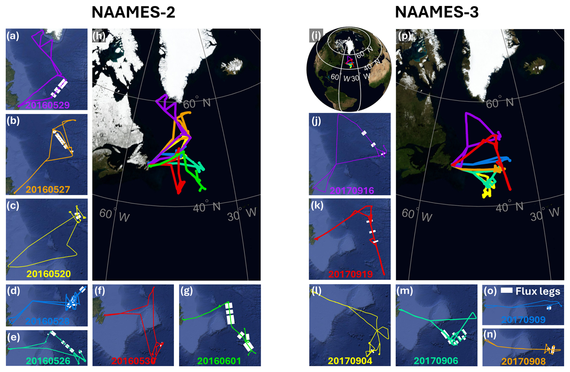
Figure 1 NAAMES flight tracks used to quantify air-sea fluxes. Panels (a)–(g) and (j)–(o) show the individual flights with flux legs indicated as white blocks (two legs in 20170906 partially overlap and are not visually distinguishable). Panels (h) and (p) show the ensemble of flux-relevant flight tracks for each NAAMES phase colored by flight number (the full set of NAAMES flight tracks are shown in Fig. S1). Panel (i) shows the geographic location of the NAAMES study area. Imagery in panels (h), (i), and (p) is © 2004 NASA Earth Observatory (Blue Marble: Next Generation). Imagery in panels (a)–(g) and (j)–(o) is © 2011 Google with terrain data from the U.S. Geological Survey and National Geospatial-Intelligence Agency (GMTED2010).

VOC mole fractions were measured on-board the C-130 by proton-transfer-reaction time-of-flight mass spectrometry (PTR-ToF-MS) during NAAMES-1 (for 4 of the 7 flights), NAAMES-2 (9 of 11 flights), and NAAMES-3 (9 of 12 flights). The employed instrument is an upgraded version of the prototype PTR-ToF-MS 4000 described by Müller et al. (2014) and manufactured by IONICON Analytic GmbH (Innsbruck, Austria). VOCs were sampled from outside the aircraft boundary layer using a winglet and a heated (50 °C) $\mathrm{1}/{\mathrm{4}}^{\prime \prime }$ surface-treated stainless-steel line (Sulfinert^®, Restek Corporation, Bellefonte, PA, USA). During NAAMES the winglet was positioned in a downward-facing orientation at the fuselage of the C-130. The inlet flow varied with ambient pressure from 15 standard liters per minute (L min⁻¹) at high altitudes to 30 L min⁻¹ at sea level. Reported analytes were calibrated via dynamic dilution of a certified compressed-gas standard (Apel-Riemer Environmental, Inc.), and sensitivities during NAAMES ranged from 320 cps ppb⁻¹ for methanol to 2206 cps ppb⁻¹ for methylethyl ketone. One-second concentration limits of detection were in the low 10s of ppt for most compounds, with an overall range of 9 ppt for toluene to 229 ppt for methanol. Zeroing was performed by passing ambient air through a Pt/Pd catalyst heated to 350 °C (Müller et al., 2014). The instrument achieved a mass resolution ($m/\mathrm{\Delta }m$, full-width half-maximum) of approximately 4000, with the mass axis calibrated through continuous addition of diiodobenzene (PerMassCal; IONICON Analytik GmbH, Innsbruck, Austria). The expected e-folding time (after accounting for inlet lag) for this instrument is approximately 0.1 s for most species targeted here but may be longer for sticky compounds (Müller et al., 2016). The NAAMES measurements were conducted at 5 Hz sampling frequency (selected as a compromise between response time, file size, and data load) with an estimated accuracy of 10 % + 5 ppt. Table 1 lists the compounds examined in this study, which include methanol (detected as CH₄O⋅H⁺ at $m/z$ 33.033), acetonitrile (C₂H₃N⋅H⁺, 42.034), acetaldehyde (C₂H₄O⋅H⁺, 45.033), methanethiol (CH₄S⋅H⁺, 49.011), acetone (C₃H₆O⋅H⁺, 59.049), dimethyl sulfide (C₂H₆S⋅H⁺, 63.026), methylethyl ketone (C₄H₈O⋅H⁺, 73.065), dimethyl sulfoxide (C₂H₆SO⋅H⁺, 79.021), benzene (C₆H₆⋅H⁺, 79.054), toluene (C₇H₈⋅H⁺, 93.070), C8 aromatics (C₈H₁₀⋅H⁺, 107.086), C9 aromatics (C₉H₁₂⋅H⁺, 121.101), and monoterpenes (C₁₀H₁₆⋅H⁺, 137.132) (Pagonis et al., 2019). The mass used to measure isoprene (C₅H₈⋅H⁺, 69.070) was affected by contamination and we therefore omit this compound. The monoterpene signal was corrected for fragmentation to $m/z$ 81.070 (∼ 50 %) and 95.086 (minor); fragmentation to $m/z$ 93.070 and 79.054 was insignificant due to the soft ionization conditions. Acetone and MEK are detected with their isomeric aldehydes (propanal; n-butanal + 2-methylpropanal). However, observations during the Atmospheric Tomography Mission (ATom) over the North Atlantic show the ketones to be dominant in this environment, with aldehyde : ketone ratios of 0.02–0.05 (propanal : acetone) and 0.16–0.23 (n-butanal : MEK; 2-methylpropanal was not detected) (Thompson et al., 2022; Apel et al., 2021; Wofsy et al., 2021). Furthermore, n-butanal is strongly fragmented (>50 %) by the first-generation PTR-ToF-MS ion funnel deployed during NAAMES and was primarily detected at $m/z$ 55.054 rather than 73.065. We therefore presume the NAAMES measurements of ∑(acetone + propanal) and ∑(MEK + n-butanal + 2-methylpropanal) to be dominated by acetone and MEK for the discussion that follows. The remaining masses above are assumed here to be dominated by the individual species listed.

Table 1 Summary of airborne VOC flux measurements during NAAMES.

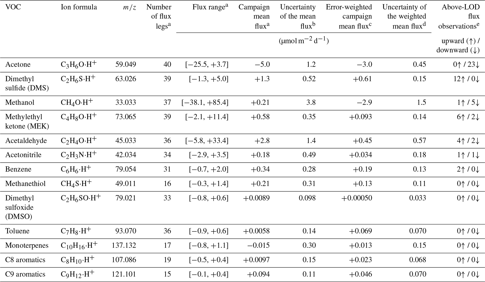
^a,c The traditional versus wavelet fluxes agree to within 30 %, including below-LOD fluxes. ^b,d 3σ uncertainty. ^b Calculated via error propagation (Taylor, 1997; see Ch. 3). ^c,d Computed following Taylor (1997; see Ch. 7). ^e Number of flux measurements that exceed the corresponding observation-specific flux LOD (3σ).

Winds were measured onboard the C-130 using the NASA Langley Turbulent Air Motion Measurement System (TAMMS) at a frequency of 5 (in 2016) and 20 Hz (in 2017). Like its previous iteration (Thornhill et al., 2003), the system uses fast-response flow-angle and temperature sensors to determine the wind with respect to the aircraft, and employs an Applanix 650 inertial navigation system (Applanix Inc.) to provide the aircraft's position, speed and attitude. Ambient air temperature measurements needed to determine true air speed are made with a Rosemount Model 102 non-deiced total air temperature sensor with a fast-response platinum sensing element (E102E4AL). Three-dimensional winds are computed from the full air motion equations (Lenschow, 1986) and corrected for aircraft motion as described by Thornhill et al. (2003) based on statistics derived from calibration maneuvers performed throughout the multi-year NAAMES EVS campaign. No additional corrections were required, and the uncertainty in the resulting wind fields is estimated at 10 %.

Other C-130 datasets employed in our analysis include flight navigation and housekeeping information (Behrenfeld et al., 2022; Bennett et al., 2020), water vapor mole fractions (LI-7200, LI-COR Inc.), and potential temperatures.

3 Ocean-air VOC exchange indicated by MBL vertical gradients

Figure 2 shows median VOC profiles over the North Atlantic as measured during NAAMES-1, 2, and 3. The observed vertical structure differs between species and reflects distinct controlling processes including air-sea exchange. For example, DMS, DMSO, and CH₃SH concentrations are enhanced near the ocean surface, consistent with their known ocean sources (Novak et al., 2022; Hoffmann et al., 2016). Monoterpenes and toluene also exhibit near-surface enhancements during NAAMES (Rocco et al., 2021; Yassaa et al., 2008). In contrast, acetone, methanol, and acetonitrile are depleted in the lowermost atmosphere, implying net ocean uptake during the sampling period. Cases with varying profile shapes across campaigns (acetaldehyde, MEK, C8/9 aromatics) or with little vertical gradient (benzene) could indicate weak, bidirectional, or seasonally varying exchange.

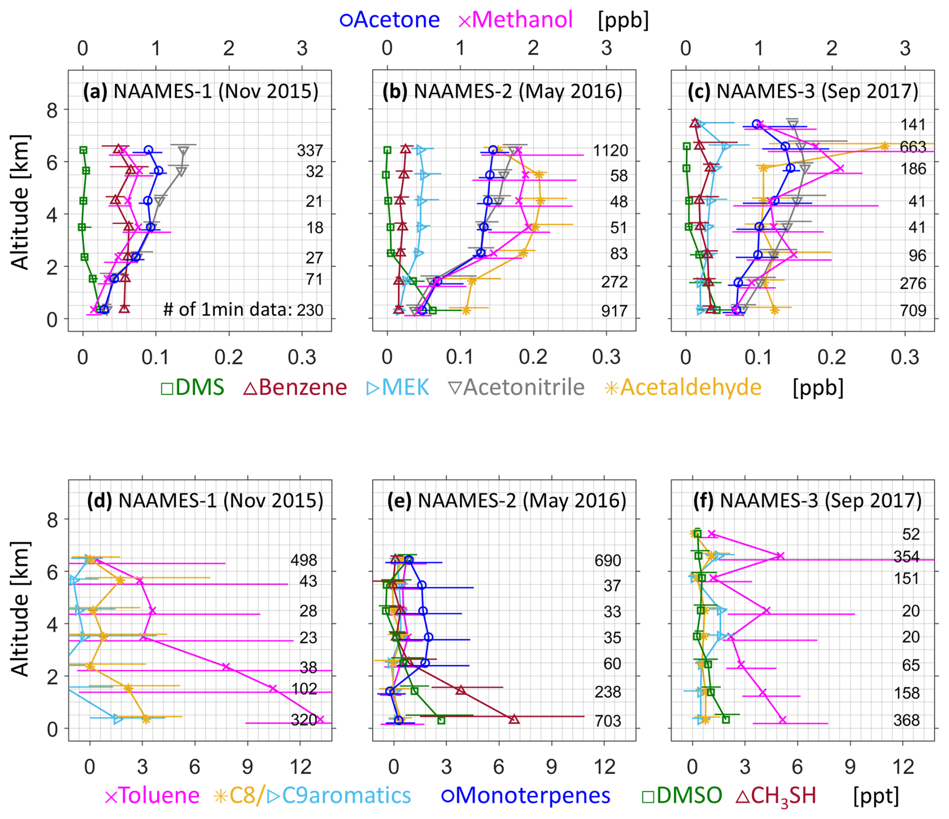
Figure 2 VOC vertical profiles observed during NAAMES-1, 2, and 3. Data plotted reflect the campaign-median concentrations (with interquartile range) in 1 km bins as measured over open ocean (east of 45° W, 48° W, and 46° W for NAAMES-1, 2, and 3, respectively) along the flight tracks shown in Fig. S1. Right-aligned values indicate the mean number of valid 1 min data points across species in each vertical bin. Acetaldehyde and methanol data during flight 20151123 (NAAMES-1) are affected by isomeric interferences and are filtered accordingly. Flight 20160520 (NAAMES-2) is pollution-influenced and excluded here to better reflect the remote marine atmosphere. Instrument background subtraction imparts a systematic uncertainty of ±5 ppt to the values plotted above but does not affect the flux analyses.

The concentration profiles are influenced to varying degrees by air-sea exchange, but they also incorporate effects from transport, atmospheric chemistry, and cloud processing. Separating these influences based on concentration measurements alone is not direct or straightforward. EC provides an avenue for direct surface-atmosphere flux quantification, and we proceed next to explore the application of this technique to the NAAMES airborne dataset.

4 Quantifying airborne eddy covariance fluxes and their uncertainties

4.1 Data pre-processing

Airborne EC analysis begins with steps for flux leg selection, signal detrending and filtering, and time-lag correction. We first temporally align the wind and VOC data on a common 5 Hz time base via nearest-neighbor matching (for the 5 Hz wind data in 2016) or bin-averaging (for the 20 Hz wind data in 2017). We next identify all prospective flux legs, defined as level (±34 m) flight intervals in the lower atmosphere, with roll and pitch less than approximately 5°, that are ∼ 3 min or more in duration (24 km at an average C-130 airspeed of 132 m s⁻¹) to ensure adequate sampling across eddy scales and a statistically robust number of data points. We also require that each leg has a quantifiable VOC-wind lag time as detailed later in this section. Table S1 lists the 44 flux legs from 13 NAAMES-2 and NAAMES-3 flights identified in this way, which average 9 min (∼ 72 km) in duration and range from 3–25 min (∼ 20–210 km) at mean sampling altitudes of 126–219 m. Mean airspeeds range from 111–157 m s⁻¹ across the flux legs, corresponding to approximately one 5 Hz data point per 22–31 m.

The resulting data subsets undergo mean-removal and detrending to isolate the scalar concentration fluctuations that are driven by turbulence. We employ 100 s (11–16 km) moving-average mean removal; as shown in the Supplement this acts as a high-pass filter to remove low-frequency, non-turbulent components (e.g., caused by air mass variability) that might not be excluded with a simple linear detrend (Novak et al., 2021; Moncrieff et al., 2005).

The time lags between scalar and wind measurements are next determined based on the maximum cross-covariance between the VOC concentration and vertical wind speed (w) within 0±50 s, first applying a 0.02 Hz high-pass filter via Fast Fourier Transform (FFT) to remove any low-frequency covariance trends. This filter enables more accurate time-lag determination but is omitted from the subsequent variance partitioning, flux, and error calculations. In multiple cases the cross-covariance for an individual flux leg lacks a sufficiently clear peak for time-lag diagnosis (Fig. 3), and we therefore employ two alternative treatments as follows. (1) Flight-specific: here the time lag is defined based on the strongest cross-covariance peak for any species across the entire flight. The 13 lags calculated in this manner range from 0.4–10.8 s. (2) Species- and leg-specific: here the time lag is allowed to be species- and flight-leg specific. For both treatments, the derived lag times primarily reflect clock offsets between the PTR-ToF-MS and wind measurement systems, which varied by flight; the physical lag time expected for the 3.3 m (0.3175 cm ID) inlet with flows exceeding 15 L min⁻¹ is <0.1 s.

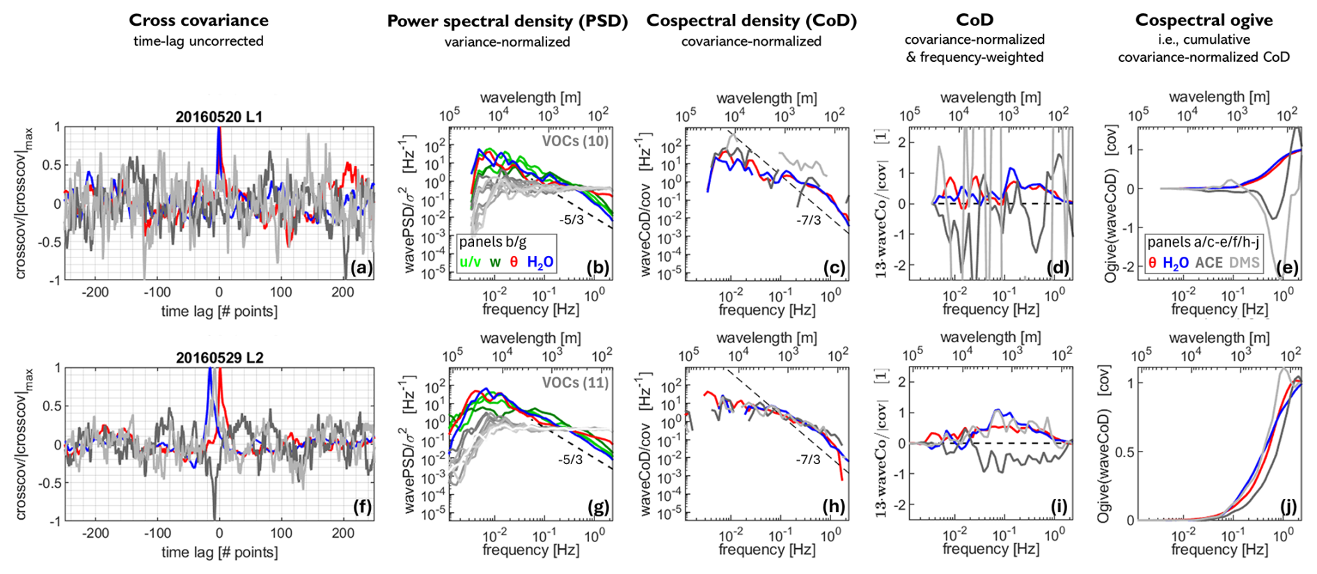
Figure 3 Example s-w cross-covariances (panels a, f) and wavelet-based spectral analyses (b–e, g–j). The top row shows an example flux leg in which clear cross-covariance peaks and well-behaved cospectra/ogives are obtained for water vapor (H₂O) and potential temperature (θ) but not for VOCs. The bottom row shows an example leg with clear cross-covariance peaks and reasonably well behaved cospectra/ogives for all plotted scalars. The impact of white noise on the VOC measurements is evident in the high-frequency range of the power spectra in panels (b) and (g). The wavelength scale is computed as the aircraft ground speed divided by frequency, without any height scaling. Line breaks in panel (c) and (h) occur where the flux power is in the opposite direction to that of the overall (net) flux value.

Treatment 1 above assumes that the targeted VOCs interact similarly with the sampling inlet and instrument, and that inter-species lag differences mainly reflect statistical artifacts. Fluxes derived in this way are conservative relative to those obtained with treatment 2, which (in addition to clock synchronization) allows for species-specific sampling effects and tends to derive the largest possible flux magnitude. In the following analysis we use treatment 1 (a single flight-specific lag applied across species) as default.

4.2 Flux derivation

EC fluxes are computed from the pre-processed, high-resolution scalar and vertical wind time series obtained above. We employ both traditional and wavelet-based flux calculations to test the robustness of our results; the wavelet approach also provides temporally- (and for airborne fluxes, spatially-) resolved information within each flux leg.

Traditional ensemble-average EC calculations are performed strictly in the time domain, with fluxes calculated from the covariance between w and the scalar at hand (s, e.g. VOC mole fraction, water vapor mole fraction, or potential temperature) over a given analysis interval:

$$\begin{array}{}\text{(1)}& f=\stackrel{\mathrm{‾}}{w^{\prime }{s}^{\prime }},\end{array}$$

where primes reflect deviations from the mean and the overbar indicates time averaging. With the above units f takes the form of a kinematic flux (e.g., ppb m s⁻¹); scaling by the atmospheric number density then converts to an areal flux (e.g., molec. cm⁻² s⁻¹). Spectral information is subsequently obtained via FFT for quality assessment.

Wavelet transformation is an alternative approach that decomposes the s and w time series into both time and frequency space (Torrence and Compo, 1998) through application of a wavelet transfer function. This yields the corresponding wavelet coefficients (W_s,W_w), with the s-w cospectrum obtained as the real part of the cross-wavelet spectrum $W_{\mathrm{s}}{W}_{\mathrm{w}}^{\ast }$ divided by its corresponding scale (Liu et al., 2007). Integrating the cospectral power across frequency scales generates the time-resolved wavelet flux series, while averaging over time collapses all the local cospectral slices into a global cospectrum that can then be compared to the FFT cospectrum associated with traditional EC. In analyses here we include the cone of influence (Torrence and Compo, 1998) to prevent systematic underestimation relative to the traditional flux estimates (Wolfe et al., 2018). Figure S2 shows that the resulting wavelet-based flux estimates agree well with traditional EC results (R² values ≥0.95; zero-intercept slopes $\in [\mathrm{0.89},\mathrm{1.07}]$; values are within 30 % in 83 % of cases).

4.3 Spectral analyses

Spectral analysis provides frequency-resolved information to diagnose EC noise effects, assess high or low frequency flux attenuation, identify dominant flux-carrying eddy scales, and compare traditional versus wavelet-based results. The Supplement file presents a full spectral analysis for the entire NAAMES airborne EC dataset, with example results shown in Fig. 3. The overall results indicate that: (1) the FFT spectra are in general agreement with the wavelet-based findings; (2) the VOC power spectra flatten out at higher frequencies, suggesting a white noise impact; and (3) the VOC-w cospectra are noisy but do not show any evidence of systematic high- or low-frequency flux loss.

4.4 Flux error budget

In this section we examine potential error sources affecting the NAAMES flux analysis, with the aim of drawing broader conclusions that can inform future airborne VOC measurements. The following processes may contribute systematic and/or random errors to the computed fluxes:

• A.

  Sensor calibration errors. A calibration bias for the VOC or vertical wind measurement would cause a systematic flux error of the same magnitude. We estimate these at 10 % each and 14 % combined (see Sect. 2).

• B.

  High-frequency attenuation. Loss of high-frequency flux contributions can arise from an insufficient sampling frequency, inadequate instrument time response, or inlet-line damping. If uncorrected, the result is a systematic flux underestimate. The NAAMES VOC-w cospectra do not show systematic evidence of such an effect when compared to those for the non-VOC scalars (Fig. 3, Supplement). Specifically, across all 44 flux windows we identify only one instance where there is any indication of high-frequency flux loss (flight 20170908 L2). It is possible that the instrument noise is obscuring attenuation in some of the other cases, but since there is no direct evidence of a systematic impact we perform no high-frequency correction and expect that other error sources are more important.

• C.

  Low-frequency losses. A sampling duration that is too short to capture the largest-scale eddies will cause a systematic flux underestimate. The ogives (plateauing at low frequencies) and 95 % eddy scales (on average <10 % of the leg length) seen during NAAMES indicate that such losses are unimportant for this study (Fig. 3, Supplement, Table S1).

• D.

  Non-stationarity. Variability contributed by larger-scale, non-turbulent motion can bias computed fluxes in a positive or negative direction. We do not view this as a predominant error source for NAAMES given the detrending approach used and given the agreement between traditional EC results and wavelet-based results (which do not require stationarity, Göckede et al., 2019).

• E.

  Uncorrelated sensor noise (USN). USN leads to random flux errors and can also cause systematic errors (e.g., via the time lag effects described next). Both aspects will be examined here.

• F.

  Time lag. When USN is large relative to the flux-driven concentration fluctuations, estimates of the wind-scalar time lag (based on their cross-covariance) may be inaccurate (Langford et al., 2015). This leads to a systematic bias in the derived flux (Sect. 4.6) and is one way that random measurement uncertainties can cause systematic flux errors.

• G.

  Turbulent stochasticity. The stochastic nature of turbulence can cause random flux errors due to incomplete statistical sampling across eddy scales. If USN and turbulent stochasticity are the predominant random error sources, the latter term can be estimated as the residual between the total flux random error and the USN-driven error:

  $$\begin{array}{}\text{(2)}& {\mathit{\sigma }}_{\mathrm{f},\mathrm{RE}}^{\mathrm{2}}={\mathit{\sigma }}_{\mathrm{f},\mathrm{USN}}^{\mathrm{2}}+{\mathit{\sigma }}_{\mathrm{f},\mathrm{turb}}^{\mathrm{2}}.\end{array}$$

Here and throughout the remaining text, we denote variances related to fluxes with a subscripted f (or f); those related to scalar quantities use a subscripted s (or s; w or w for vertical wind). Of the above errors, A and G are straightforward to assess while B–D are not expected to predominate for NAAMES. In the following sections we therefore focus on terms E and F and determine their impacts on the flux error budget by: (1) Quantifying the total flux random error and the flux random error caused by USN; and (2) conducting noise perturbation experiments to characterize the random versus systematic impacts of USN and time-lag uncertainty on the computed fluxes. The same experiments then allow us to quantify the relative effects of USN and turbulent stochasticity on the flux signal-to-noise ratio.

4.5 Flux random error: quantification, partitioning, and impact on signal-to-noise ratio

We tested four empirical approaches for computing the total flux random error (σ_f,RE), based on: (i) the standard deviation of the scalar-wind covariance away from the true time lag (Spirig et al., 2005; Wienhold et al., 1995); (ii) a modified version of (i) that also accounts for cross-covariance offsets (Langford et al., 2015); (iii) the $\stackrel{\mathrm{‾}}{w^{\prime }{s}^{\prime }}$ standard error (Wolfe et al., 2015); and (iv) the variance of the scalar-wind covariance (Bendat and Piersol, 2010; Finkelstein and Sims, 2001). Results from these approaches agree closely (R>0.82) across NAAMES VOCs, with approach (iii) giving generally lower error estimates. In what follows we report flux random errors based on the Spirig-Wienhold approach (i), which range from 0.006–7 ppt m s⁻¹ (1σ; 0.02–27 µmol m⁻² d⁻¹) for VOC cases in which the traditional versus wavelet fluxes agree to within 30 %. These random errors (Fig. 4) are insensitive to time lag uncertainties; as will be seen, the same is not true of the systematic error component.

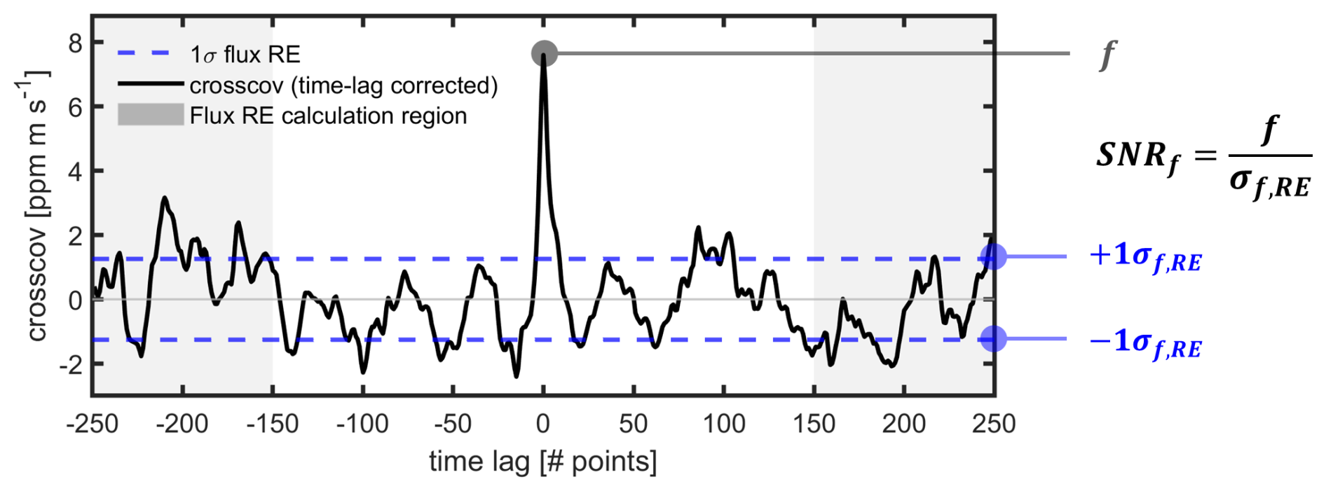
Figure 4 H₂O scalar-wind cross-covariance (crosscov) from NAAMES flight 20160520 L1, illustrating the flux signal-to-noise ratio (SNR_f). The flux random error (σ_f,RE) is estimated using the Spirig-Wienhold approach (Spirig et al., 2005; Wienhold et al., 1995). Figure format follows Langford et al. (2015).

The flux random errors arise from both USN and turbulent stochasticity (Eq. 2). To quantify the USN contribution (σ_f,USN), we first use autocovariance analysis (Lenschow et al., 2000) to partition the variability in scalar concentration (mean-removed and detrended) or in vertical wind to its USN versus atmospheric contributions (e.g., ${\mathit{\sigma }}_{\mathrm{s},\mathrm{tot}}^{\mathrm{2}}={\mathit{\sigma }}_{\mathrm{s},\mathrm{USN}}^{\mathrm{2}}+{\mathit{\sigma }}_{\mathrm{s},\mathrm{turb}}^{\mathrm{2}}$). Any negative contributions derived in this way are set to zero with the sum conserved. Figure S3 shows that during NAAMES the VOC scalar variance is dominated by USN (98 % of $\frac{{\mathit{\sigma }}_{\mathrm{s},\mathrm{USN}}^{\mathrm{2}}}{{\mathit{\sigma }}_{\mathrm{s},\mathrm{tot}}^{\mathrm{2}}}$ ratios exceed 50 %), whereas turbulence dominates the observed scalar variance for H₂O, θ, and w – consistent with the power spectra behavior. We next construct an ensemble of Gaussian white noise realizations (a reasonable treatment based on the spectral analyses) with USN variance (${\mathit{\sigma }}_{\mathrm{s},\mathrm{USN}}^{\mathrm{2}}$) prescribed according to the autocovariance results for each scalar. For each realization, we calculate the standard deviation of the cross-covariance between the resulting noise timeseries and w (away from the true time lag). As the scalar here is entirely noise, this standard deviation is equivalent to σ_f,USN in Eq. (2). Ten such realizations are averaged to obtain the final σ_f,USN values for each scalar.

The empirical approach outlined above combines ideas from Lenschow et al. (2000), Langford et al. (2015), and Wolfe et al. (2015), and is referred to as LLW hereafter. When we compare the resulting σ_f,USN estimates to the σ_f,RE values obtained earlier we find that the total flux random error is dominated by the USN contribution for VOCs (92 % of $\frac{{\mathit{\sigma }}_{\mathrm{f},\mathrm{USN}}^{\mathrm{2}}}{{\mathit{\sigma }}_{\mathrm{f},\mathrm{RE}}^{\mathrm{2}}}$ ratios exceed 50 %, with smaller ratios for species with better-resolved fluxes) but by turbulent stochasticity for θ and H₂O. This flux-based finding aligns with the concentration-based autocovariance results above and shows that the VOC flux measurements are occurring in a noise-limited regime. The situation therefore differs from that encountered for air-sea flux measurements of CO₂, where sampling uncertainties are often the principal random error source (Dong et al., 2021).

We can next define a flux signal-to-noise ratio as SNR${}_{\mathrm{f}}=\frac{f}{{\mathit{\sigma }}_{\mathrm{f},\mathrm{RE}}}$ (Fig. 4). SNR_f is analogous to the conventional concentration-based SNR definition: there, the signal is the measured concentration and the noise is the instrument precision, while here the signal is the measured flux and the noise is the total flux random error (due to USN and turbulent stochasticity). The flux limit of detection (LOD) can then be defined as the flux at which SNR_f=3.

Analyses above showed for the VOCs measured during NAAMES that USN has a large impact on the total flux random errors; as a result, only 13 % of the derived fluxes have SNR_f≥3. The NAAMES VOC dataset thus presents a case where comparatively large USN contributes to low SNR_f and elevated flux LODs. Below, we conduct noise perturbation experiments to quantify the systematic and random impacts of USN on the derived fluxes and on SNR_f, with a goal of clarifying sensor requirements for future airborne flux missions.

4.6 Sensor noise causes systematic flux errors: Results from noise perturbation experiments

The H₂O concentration measurements from 11 NAAMES flux legs during 3 flights (20160528, 20160529, 20160601) exhibit well-behaved power spectra and we use them here as archetypical flux-driven signals without significant noise impacts. We impose Gaussian white noise (${\mathit{\sigma }}_{\mathrm{imposed}}^{\mathrm{2}}$) onto these selected concentration signals at five different power levels according to ${\log }_{\mathrm{10}}\left(\frac{\stackrel{\mathrm{‾}}{{\left[{\mathrm{H}}_{\mathrm{2}}\mathrm{O}\right]}^{\mathrm{2}}}}{{\mathit{\sigma }}_{\mathrm{imposed}}^{\mathrm{2}}}\right)=\mathrm{4.5},\mathrm{3.5},\mathrm{2.5},\mathrm{1.5},\mathrm{0.5}$, with the levels selected such that results range from H₂O-like to VOC-like in the context of NAAMES. For a given signal and noise level, 500 random noise realizations are conducted (total: 27 500). These simulations are conducted separately for scenarios in which the scalar-wind time lag is (i) known and prescribed, and (ii) computed separately for each realization.

When the scalar-wind time lag is known and prescribed, the 500 fluxes derived in this way at a given noise level approximate a normal distribution centered approximately on the true value – with increasing spread at higher noise (Fig. 5). Conversely, when the time lag is computed separately for each realization, the 500-flux ensemble is no longer centered on the true value for the higher noise scenarios. Rather, a ghost peak appears – with a subset of the ensemble exhibiting spurious fluxes in the opposite direction of around the same magnitude. Eventually, both mirrored populations exceed the true flux magnitude, as random spikes in the noise-wind cross-covariance exceed the actual H₂O-wind covariance. In such cases, the true flux is obscured by the noisy cross-covariance, and searching for the maximum on a case-by-case basis tends to overestimate the flux magnitude with random direction. The phenomenon parallels the mirroring described by Langford et al. (2015). In the high-noise limit, we see from Fig. 5 that the average over an ensemble of measurements converges to approximately the true flux in the prescribed time-lag scenario, but it converges to near-zero in the non-prescribed scenario. In this way, random errors in the form of USN can yield systematic flux errors by inhibiting accurate determination of the scalar-wind time lag. For situations where a significant number of the fluxes are near or below the LOD, time lags should when possible be prescribed (e.g., from proximate higher-flux periods, or based on higher-flux co-measured compounds) to avoid imposing a systematic bias on the results.

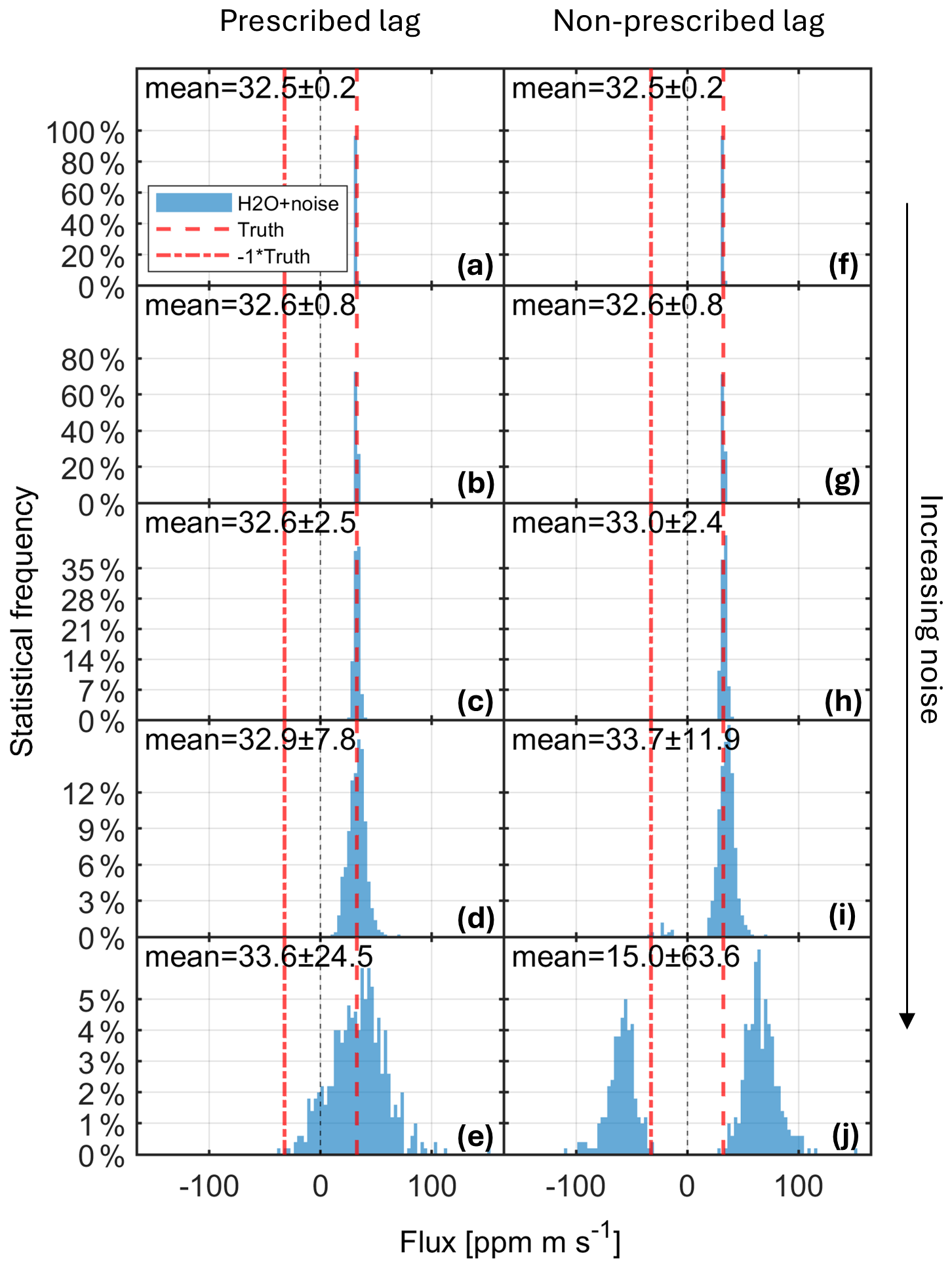
Figure 5 Flux histograms for the noise perturbation ensemble. H₂O fluxes from NAAMES flight 20160601 L1 are subjected to five different noise levels (${\mathit{\sigma }}_{\mathrm{imposed}}^{\mathrm{2}}$) according to ${\log }_{\mathrm{10}}\left(\frac{\stackrel{\mathrm{‾}}{{\left[{\mathrm{H}}_{\mathrm{2}}\mathrm{O}\right]}^{\mathrm{2}}}}{{\mathit{\sigma }}_{\mathrm{imposed}}^{\mathrm{2}}}\right)=\mathrm{4.5},\mathrm{3.5},\mathrm{2.5},\mathrm{1.5},\mathrm{0.5}$. Results are shown for scenarios in which the scalar-wind time lag is known (−2.2 s) and prescribed (a)–(e) and in which the time lag is determined independently (0±10 s search window) for each flux derivation (f)–(j).

For the duration of the noise perturbation analysis here we proceed with the prescribed time-lag results. For each realization, the spread across the 500-member flux ensemble then characterizes the uncertainty associated with the contaminated H₂O flux that is due to the imposed random noise: i.e., it estimates the same σ_f,USN quantity that was derived earlier via LLW.

4.7 Sensor noise impacts on random flux errors

The results from the noise perturbation experiments allow us to empirically assess the propagation of scalar-based errors to flux-based errors that has been theoretically derived and applied in previous studies (Deventer et al., 2019; Wolfe et al., 2018; Langford et al., 2015; Peltola et al., 2014; Mauder et al., 2013; Neftel et al., 2007):

$$\begin{array}{}\text{(3)}& {\mathit{\sigma }}_{\mathrm{f},\mathrm{USN}}={\displaystyle \frac{{\mathit{\sigma }}_{\mathrm{w}}}{\sqrt{N}}}{\mathit{\sigma }}_{\mathrm{s},\mathrm{USN}}.\end{array}$$

Here, σ_w is the standard deviation of the vertical wind speed and N is the number of data points. Equation (3) takes a reduced form for NAAMES since USN for the wind measurement is negligible relative to that for the other scalars examined (Rannik et al., 2016).

Plotting σ_f,USN as a function of σ_s,USN for the noise perturbation ensemble (Fig. 6) suggests a power law relation y=Ax^K. A linear regression between log ₁₀σ_f,USN and log ₁₀σ_s,USN for each flux leg reveals a consistent K ∼ 1 (Fig. S4a), indicating a simple linear correlation y=Bx throughout the data range. The resulting slope B is within 4 % of $\frac{{\mathit{\sigma }}_{\mathrm{w}}}{\sqrt{N}}$ (Fig. S4b), with the NAAMES θ observations following the same leg-specific linear correlations as the contaminated and native H₂O data (Fig. 6). The regressions thus empirically validate the linearity and coefficients embedded in Eq. (3).

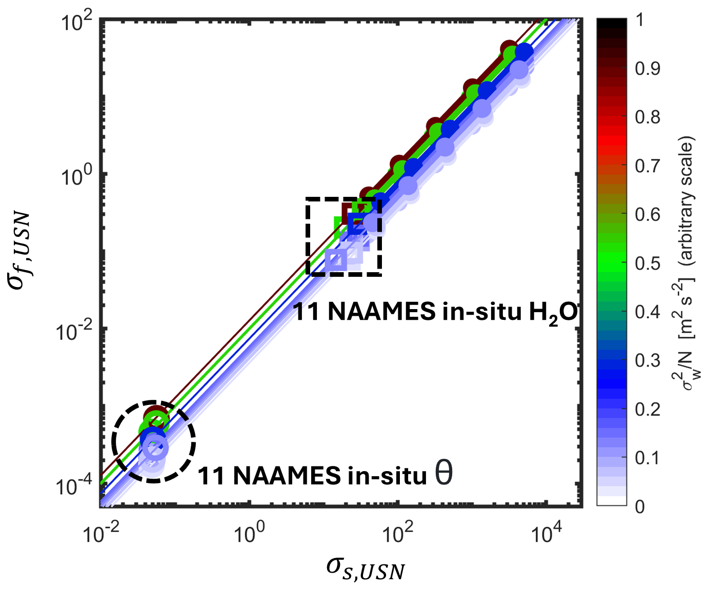
Figure 6 Impact of uncorrelated sensor noise on flux random errors. Results are shown for the noise perturbation ensemble described in-text (filled circles), for the uncontaminated NAAMES H₂O observations (squares), and for the NAAMES θ observations (hollow circles). Each plotted value for the noise perturbation ensemble reflects the mean across all 500 members (standard deviations are smaller than the data points and thus not visible). See Fig. S4 for regression statistics.

4.8 Flux signal-to-noise ratio: impact of noise versus turbulence

Substituting Eq. (3) into Eq. (2), normalizing by f², and rearranging, we obtain:

$$\begin{array}{}\text{(4)}& {\mathrm{SNR}}_{\mathrm{f}}={\left({\displaystyle \frac{{\mathit{\sigma }}_{\mathrm{w}}^{\mathrm{2}}}{N{x}^{\mathrm{2}}}}+{\displaystyle \frac{{\mathit{\sigma }}_{\mathrm{f},\mathrm{turb}}^{\mathrm{2}}}{f^{\mathrm{2}}}}\right)}^{-\mathrm{0.5}},\end{array}$$

where $x=\frac{\mathrm{|}f\mathrm{|}}{{\mathit{\sigma }}_{\mathrm{s},\mathrm{USN}}}$ is used as an independent variable such that: (i) all scalars employ the same scale, and (ii) each 500-member ensemble is normally distributed in x and can be represented through its mean ± standard deviation. ${\mathit{\sigma }}_{\mathrm{w}}^{\mathrm{2}}$ and N are leg-specific quantities reflecting the turbulent regime and the sampling duration, respectively. σ_f,turb is computed as a residual via Eq. (2). The $\frac{{\mathit{\sigma }}_{\mathrm{f},\mathrm{turb}}}{f}$ ratio quantifies the flux (relative) random error arising from turbulent stochasticity, and is affected by factors including boundary layer depth, measurement height, and sampling duration (Wolfe et al., 2018; Lenschow et al., 1994). Thus, for a given meteorological regime and sampling plan, it is mainly $x=\frac{\mathrm{|}f\mathrm{|}}{{\mathit{\sigma }}_{\mathrm{s},\mathrm{USN}}}$ that differentiates the SNR_f behavior of different scalars.

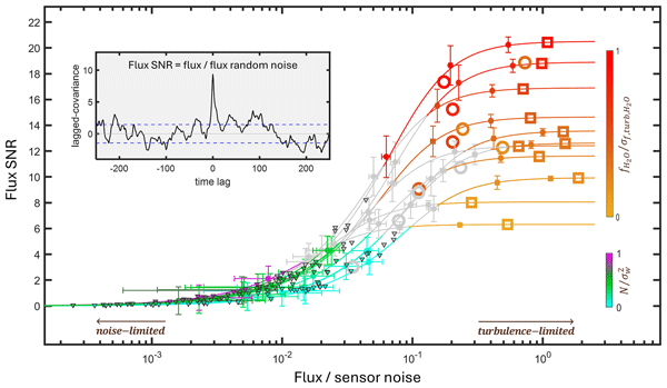
Figure 7a plots SNR_f as a function of x (Fig. S5 shows the same data on a log-log scale). Each curve shows the SNR_f:x dependence for a given flux leg with its associated duration and turbulent characteristics. The impact of USN decreases from left to right so that the derivation of SNR_f in Eq. (4) is dominated by $\frac{{\mathit{\sigma }}_{\mathrm{w}}^{\mathrm{2}}}{N{x}^{\mathrm{2}}}=\frac{{\mathit{\sigma }}_{\mathrm{w}}^{\mathrm{2}}{\mathit{\sigma }}_{\mathrm{s},\mathrm{USN}}^{\mathrm{2}}}{N{f}^{\mathrm{2}}}$ to the left (noise-limited regime) and by $\frac{{\mathit{\sigma }}_{\mathrm{f},\mathrm{turb}}^{\mathrm{2}}}{f^{\mathrm{2}}}$ to the right (turbulence-limited). The spread between curves reflects the differing meteorology, sampling conditions, and flux magnitudes across legs.

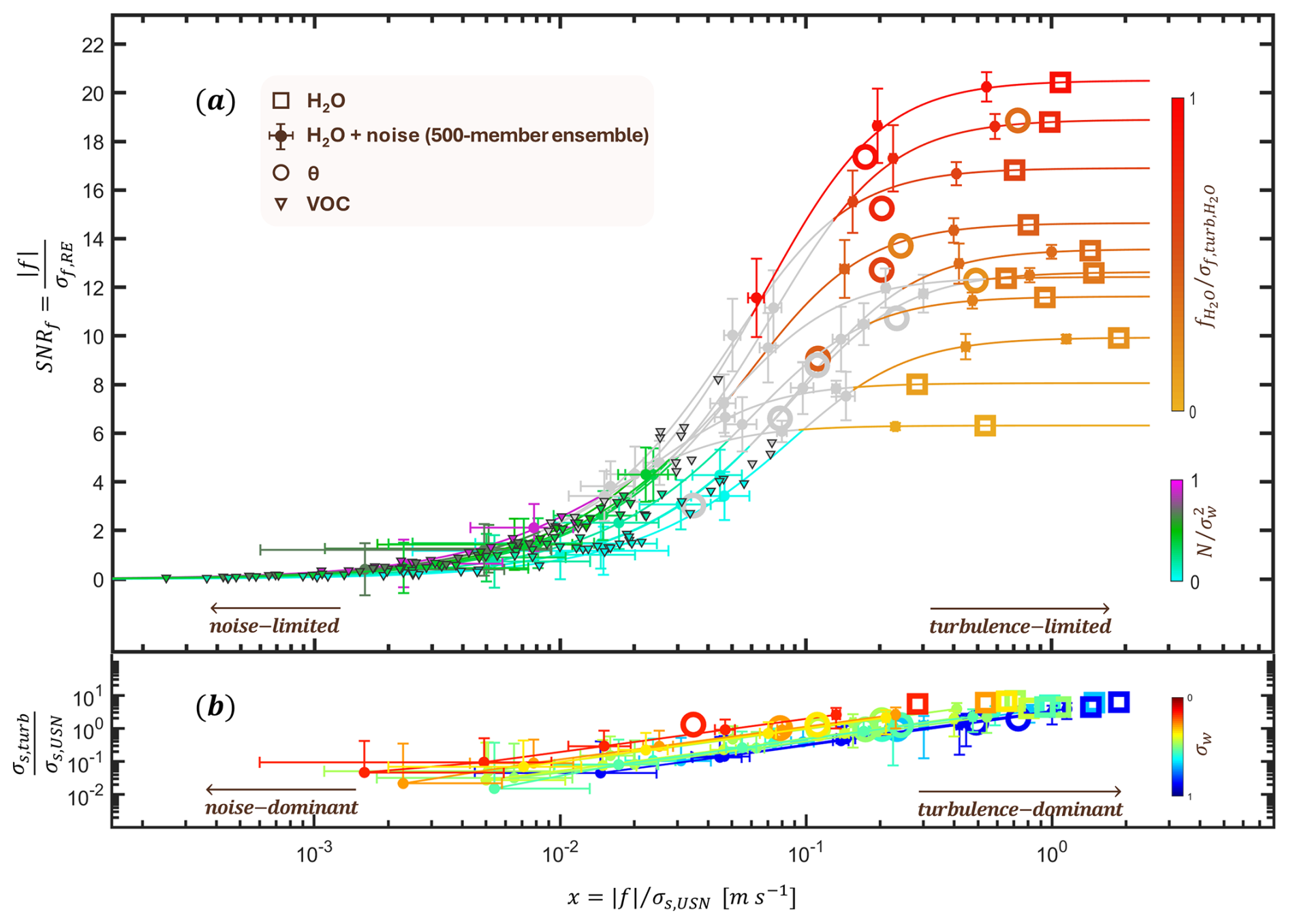
Figure 7 (a) Flux SNR (SNR_f) as a function of the flux : USN ratio. The curves visualize the SNR_f–x relationship based on Eq. (4) for the 11 analyzed flux legs, and are colored to indicate noise-limited (bottom colorbar), transitional (grey), and turbulence-limited (top colorbar) regimes. Datapoints indicate the noise perturbation ensemble (filled circles; 500-member mean and standard deviation) along with the NAAMES H₂O (hollow squares), θ (hollow circles), and VOC (triangles) observations. (b) Ratio of the turbulent- to USN-driven scalar concentration variability ($\frac{{\mathit{\sigma }}_{\mathrm{s},\mathrm{turb}}}{{\mathit{\sigma }}_{\mathrm{s},\mathrm{USN}}}$) as a function of the flux : USN ratio. Plotting conventions follow those of panel (a), with the noise perturbation ensemble represented by the 500-member median and interquartile range, and colors indicating the standard deviation of the vertical wind speed. σ_s,USN and σ_s,turb are derived from the variance partitioning analysis described in-text with negative values set to zero. Zero and negative values are omitted from the logarithmic scales. All fluxes employ traditional EC estimates with flight-specific lag times. Color bars use arbitrary scales.

The original H₂O flux observations (hollow squares) fall on the right-hand side of the corresponding leg-specific curves. The contaminated datapoints then define the transition, under those sampling conditions, to a noise-dominated regime. The in-situ θ (hollow circles) and VOC (triangles) fluxes for the same set of flux legs fall within the overall envelope delineated by the noise-contaminated H₂O data. This confluence demonstrates the broader representativeness of the plotted function curves: they define an SNR space that all scalars measured under similar sampling conditions should fall within.

Langford et al. (2015) defined an analogous SNR $\left(\frac{{\mathit{\sigma }}_{\mathrm{s},\mathrm{turb}}^{\mathrm{2}}}{{\mathit{\sigma }}_{\mathrm{s},\mathrm{USN}}^{\mathrm{2}}}\right)$ for scalar concentration variance (${\mathit{\sigma }}_{\mathrm{s},\mathrm{tot}}^{\mathrm{2}}$) that is related to the figure of merit Q $\left(\frac{{\mathit{\sigma }}_{\mathrm{s},\mathrm{USN}}}{{\mathit{\sigma }}_{\mathrm{s},\mathrm{turb}}}\right)$ proposed earlier by Lenschow and Kristensen (1985). Figure 7b plots the square root of the Langford SNR as a function of x for the same set of data as shown in panel (a). Together, Fig. 7a–b thus conveys an overall transition in air-sea flux measurements with varying $x=\frac{\mathrm{|}f\mathrm{|}}{{\mathit{\sigma }}_{\mathrm{s},\mathrm{USN}}}$. To the left is the noise-limited regime, where USN dominates σ_s,tot, and SNR_f is likewise controlled by USN in a manner that is modulated by turbulence and sampling. To the right, σ_s,tot is turbulence-driven, and SNR_f approaches a maximum value that is limited by the randomness of that turbulence. The NAAMES H₂O fluxes are well within the turbulence-limited regime, while the θ fluxes fall mostly in the turbulence-limited regime and partly in the transition regime. The majority of the in-situ VOC measurements exhibit behavior resembling that of severely noise-contaminated H₂O data and fall within the noise-limited regime.

The results in Fig. 7 provide a framework that can be used to assess whether an instrument's noise performance is sufficient for a given flux application and desired SNR_f. That is, for an expected flux magnitude, the plotted curves can be used to identify the maximum σ_s,USN that is likely to yield an appropriate SNR_f under the NAAMES sampling conditions. For the 11 actual flux legs examined in Fig. 7, 17 % of the VOC fluxes have SNR_f>3; for example, the mean (± SD) SNR_f value for acetone is 3.35±1.77 but just 0.53±0.51 for monoterpenes. We find that if USN was lowered by a factor of 7–23, 75 % of these VOC fluxes would exceed SNR_f=3. A 10–20× advance in instrumental noise performance compared to the PTR-ToF-MS deployed during NAAMES would therefore provide significant benefits in our ability to quantify ocean-air VOC fluxes.

5 NAAMES airborne VOC fluxes

We proceed to examine the VOC fluxes quantified during NAAMES, employing the flight-specific lag times as best estimates based on the results in Sect. 4.6. Table 1 lists the mean flux, LOD, and number of above-LOD flux detections for each VOC during NAAMES. Flux legs that pass the selection criteria outlined earlier all occur during NAAMES-2 (May/June 2016) and NAAMES-3 (September 2017).

Across VOCs, acetone and DMS have the greatest number of flux measurements with magnitudes exceeding the corresponding observation-specific LOD (Table 1). The fraction of above-detection fluxes for other species ranges from 0 %–21 %. However, analyses above showed that the NAAMES VOC flux errors and LODs are dominated by random USN effects, and it follows that these uncertainties are reduced through averaging. Accordingly, we see in Table 1 that in some cases the magnitude of the campaign-mean flux (and/or the error-weighted mean flux) exceeds its uncertainty level – even with just a few above-detection flux measurements. These compound-specific results are discussed further in the next sections. In all cases the limited number of flux observations and the regional sampling during NAAMES mean that results need to be interpreted with caution in terms of their broader spatial/temporal representativeness.

5.1 Acetone deposition and DMS emissions: Wind and biological controls

The measured acetone and DMS fluxes are plotted by leg in Fig. 8. For acetone, detectable fluxes are all downward and the campaign-mean exchange rate is −5.0 µmol m⁻² d⁻¹ [propagated 3σ uncertainty: ±1.2 µmol m⁻² d⁻¹]. The corresponding error-weighted mean flux is −3.0 [±0.45] µmol m⁻² d⁻¹. These values are comparable to prior shipborne EC results from the North Atlantic high latitudes (−4.8 to −11 µmol m⁻² d⁻¹ from 40–65° N) (Yang et al., 2014a, b). However, the global ocean acetone flux is heterogeneous (Wang et al., 2020) and a net source has been reported over the subtropical and southern Atlantic (Yang et al., 2014b; Taddei et al., 2009).

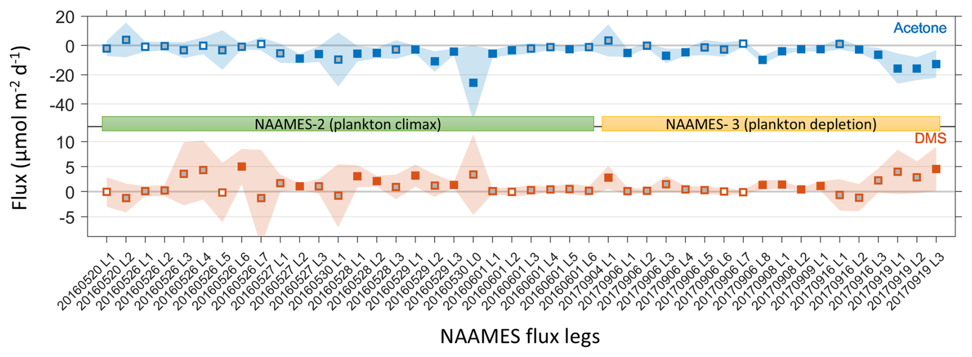
Figure 8 Airborne fluxes of acetone and DMS measured during NAAMES. Solid squares show EC-based estimates that (i) agree with the wavelet-based results to within 30 % and (ii) are above the corresponding LOD. White-filled squares indicate values where condition (i) is not met; grey-filled squares indicate values where (i) is met but (ii) is not met.

Ocean-atmosphere VOC fluxes are driven both by the air-sea mixed layer concentration difference and by the associated exchange velocity (Liss and Slater, 1974), and the airborne acetone fluxes from NAAMES reveal the influence of wind speed on this exchange. Specifically, during both NAAMES-2 and NAAMES-3 the strongest acetone fluxes occurred when horizontal wind speeds were highest (flight 20160530: ∼ 24 m s⁻¹; 20170919: ∼ 12 m s⁻¹). Figure 8 shows that the largest September fluxes for DMS likewise occurred during flight 20170919. This is consistent with the NAAMES-3 cruise results, where wind was found to be the main driver of DMS flux variability (Bell et al., 2021).

All of the airborne DMS fluxes measured during NAAMES that exceed the LOD are upward, out of the ocean. The campaign-mean flux of +1.3 [±0.52] (error-weighted mean: +0.61 [±0.15]) µmol m⁻² d⁻¹ matches ship-based EC results in the North Atlantic (40–65° N) from the HiWinGS mission during fall 2013 (mean: +1.5 µmol m⁻² d⁻¹) (Kim et al., 2017). DMS emissions estimated from the seawater concentrations measured during NAAMES-2 and NAAMES-3 ranged from +0.1 to +48 µmol m⁻² d⁻¹, with a mean of ∼ 7 µmol m⁻² d⁻¹ (Bell et al., 2021). Surface EC measurements from the North Atlantic during other seasons (+2.7 to +18.1 µmol m⁻² d⁻¹) (Land et al., 2014; Miller et al., 2009; Marandino et al., 2008) have also tended to be higher than the NAAMES airborne results.

The NAAMES airborne DMS fluxes are generally higher and more variable in spring 2016 (NAAMES-2) than in fall 2017 (NAAMES-3; Fig. 8), and this pattern aligns with the distinct biological regimes at these times (Behrenfeld, 2010). NAAMES-2 occurred during the phytoplankton climax phase with a median chlorophyll-a concentration in the study area of 1.3 mg m⁻³ (interquartile range: 0.7–2.2 mg m⁻³) and highly variable dissolved DMS concentrations (mean ± standard deviation: 3.9±2.7 nM) (Bell et al., 2021). NAAMES-3 occurred during the phytoplankton depletion phase when chlorophyll-a concentrations were far lower (0.3 [0.2–0.8] mg m⁻³) and dissolved DMS concentrations were more uniform (3.1±1.0 nM) (Bell et al., 2021). The greater dissolved DMS variability during NAAMES-2 has been attributed to the combined effects of elevated biological activity and wind-driven dilution of sea-surface concentrations (Bell et al., 2021). The strong horizontal winds during NAAMES-2 thus affected the air-sea DMS fluxes both directly (via more efficient air-sea exchange) and indirectly (via dilution of the dissolved concentrations).

5.2 Other VOCs

Of the remaining VOCs, acetaldehyde and MEK exhibit the clearest signatures of air-sea exchange, with 17 % and 21 % of individual flux measurements falling above the associated detection limit (Table 1).

• Acetaldehyde. Bidirectional air-sea exchange of acetaldehyde has been reported for this region based on shipborne EC during the Fall 2012 AMT-22 mission (mean: 0.8 µmol m⁻² d⁻¹) (Yang et al., 2014b). The NAAMES airborne results likewise indicate bidirectional exchange, with 4 upward and 2 downward above-LOD fluxes. The campaign-mean flux of +2.8 [±1.4] (error-weighted mean: +0.45 [±0.57]) µmol m⁻² d⁻¹ from NAAMES also falls within the spring/fall range for the subarctic Atlantic that has been predicted by global models (0–7 µmol m⁻² d⁻¹) (Wang et al., 2019; Millet et al., 2010).

• MEK. Prior vertical surveys over the tropical Pacific and in the remote southern hemisphere revealed enhanced MEK near the ocean surface, suggesting an oceanic source (Brewer et al., 2020). Air-sea exchange modeling for the Southern Ocean implies a net emission of ∼ 0.1 µmol m⁻² d⁻¹ based on a dissolved concentration of 0.88 nM (Brewer et al., 2020; Schlundt et al., 2017). The NAAMES airborne fluxes over the Subarctic Atlantic are predominantly upward (6 upward and 2 downward above-LOD values), and the campaign-mean oceanic emission of +0.58 [±0.35] (error-weighted mean: +0.093 [±0.14]) µmol m⁻² d⁻¹ is on the same order as the Brewer et al. (2020) estimates.

  Methanol, acetonitrile, and benzene feature 2–6 individually-detectable fluxes, while individual flux observations for the remaining VOCs all fall below the corresponding single-measurement LOD values. Nevertheless, by averaging results we can reduce uncertainties in the mean measured fluxes and draw comparisons to prior studies.

• Methanol. Methanol has one detectable upward flux under high wind speeds (+85.4 µmol m⁻² d⁻¹ on flight 20160530) and five detectable downward fluxes (−7.2, −9.0, −9.5, −11.4, and −38.1 µmol m⁻² d⁻¹). The campaign-mean exchange rate of +0.21[±3.8] and error-weighted mean of −2.9[±1.5] µmol m⁻² d⁻¹ are both smaller than the deposition fluxes detected by shipborne EC over the Northeast Atlantic (AMT-22 mean: −15 µmol m⁻² d⁻¹, Fall 2012) and the Subarctic Atlantic (HiWinGS mean: −12.3 µmol m⁻² d⁻¹, Fall 2013) (Yang et al., 2013, 2014a, b). The mean of the five detectable downward fluxes measured during NAAMES (−15 µmol m⁻² d⁻¹), however, is very similar to those prior shipborne EC results.

• Methanethiol. Based on monthly seawater concentrations extrapolated from field observations, Wohl et al. (2024) calculated CH₃SH emission fluxes for the subarctic Atlantic that generally exceeded 1–3 µmol m⁻² d⁻¹. The NAAMES flux is approximately an order of magnitude lower than that, averaging +0.21 [±0.31] µmol m⁻² d⁻¹ (error-weighted mean: 0.13 [±0.11] µmol m⁻² d⁻¹). Nevertheless, the campaign-mean DMS:methanethiol flux ratio of 4–5 is in-line with prior EC-based (5.5) (Novak et al., 2022) and calculated values (3.2–6.1) (Lawson et al., 2020; Kettle et al., 2001).

• Benzene/Toluene/C8 aromatics. From measured seawater concentrations in the Southern Ocean and Arctic, Wohl et al. (2023) inferred sea-to-air benzene and toluene emission rates of approximately +0.03 µmol m⁻² d⁻¹. Meanwhile, mesocosm studies in the Southwest Pacific Ocean suggested benzene, toluene, and C8 aromatic fluxes of +1.1, +0.9, and +0.8 µmol m⁻² d⁻¹, respectively (Rocco et al., 2021). The mean and error-weighted mean fluxes from NAAMES (including their uncertainty ranges) are significantly lower than the mesocosm results and are closer to the Wohl et al. (2023) estimates (Table 1).

• Acetonitrile. Overall, it seems clear that the ocean acts as a net sink for acetonitrile as its concentrations are usually depleted in the MBL (de Gouw et al., 2003; Li et al., 2003; Singh et al., 2003b). Singh et al. (2003b) inferred an oceanic deposition flux of 0.2 µmol m⁻² d⁻¹ based on observations over the Pacific Ocean, but other work has shown that the marine CH₃CN sink varies strongly with location (de Gouw et al., 2003). The airborne observations during NAAMES provide some indication of bidirectional exchange (with 1 upward and 1 downward above-LOD fluxes), but the campaign-mean and error-weighted mean exchange rates are statistically indistinguishable from zero – with uncertainties that encompass the Singh et al. (2003b) estimate (Table 1).

• Monoterpenes. Prior shipborne EC measurements in the North Atlantic revealed bidirectional fluxes for monoterpenes (averaging +0.04 µmol m⁻² d⁻¹) (Kim et al., 2017). No detectable monoterpene fluxes were measured and the campaign-mean exchange rate is likewise not distinguishable from zero (Table 1).

• DMSO/C9 aromatics. To our knowledge there have not been any reported air-sea exchange rates for these species. Their fluxes were undetectable during NAAMES, and the uncertainty range for the campaign-mean results suggests that any air-sea exchange that did occur had a magnitude less than approximately 0.1 µmol m⁻² d⁻¹ (Table 1). However, it is possible that wall interactions may have inhibited flux detectability for these lower-volatility species.

5.3 Potential impact of flux divergence

Prior studies have examined the role of vertical flux divergence for VOCs in the MBL, focusing on DMS (e.g., Bandy et al., 2002; Stevens et al., 2003; Faloona et al., 2005; Conley et al., 2009) and its oxidation products (Novak et al., 2021). Processes that can lead to a change in EC-measured fluxes with height include: (i) photochemical oxidation or production of a given VOC; (ii) entrainment of VOC-depleted or VOC-enriched air from aloft; (iii) horizontal advection/changing source footprint with height; or (iv) cloud processing. The sign of the expected effect varies depending on the dominant process and on the source-sink profile for a given VOC. Flux legs analyzed here range in elevation from 126–219 m, and based on the gradients reported in the above-cited studies we expect air-sea exchange to be the predominant influence within that range. However, NAAMES did not include sufficient multi-level sampling for us to quantify the impact of vertical flux divergence across the study, and we cannot rule out its role entirely.

6 Remarks and outlook

A primary focus of this work has been to characterize the impacts of uncorrelated sensor noise (USN) on eddy covariance (EC) flux measurements and errors. Our analysis employed the NAAMES airborne dataset and examined air-sea VOC fluxes over the North Atlantic; more broadly, the results shed light on EC sampling regimes where flux magnitudes are modest relative to the noise performance of the sensor. Here we built on prior work (Langford et al., 2015) to quantify the systematic and random flux errors that arise from random instrument errors in the form of USN. The random flux errors propagate linearly from USN, while systematic biases also occur when USN obscures the true wind-scalar time lag. We showed that in a noise-limited regime, an ensemble of flux measurements converges to the truth when the time lag is accurately prescribed – for example, from proximate higher-flux periods, or based on higher-flux compounds. The same is not true when time lags are calculated separately based on each individual flux observation, since under noise-limited conditions the average in this case converges to zero rather than to the true flux. We therefore recommend the former approach when it is feasible.

The impact of measurement noise is typically described in terms of a signal-to-noise ratio (SNR), which inherently relates a strength-of-signal to an associated noise level. In concentration space SNR is computed as the ratio between a concentration magnitude and its random error; however, this quantity is not directly relevant to fluxes because the signal of interest is then no longer the concentration magnitude but rather its turbulent fluctuations. Langford et al. (2015) derived a concentration variance SNR as the ratio between turbulence-driven concentration variability and noise driven concentration variability ($\frac{{\mathit{\sigma }}_{\mathrm{s},\mathrm{turb}}^{\mathrm{2}}}{{\mathit{\sigma }}_{\mathrm{USN}}^{\mathrm{2}}}$); this quantity is more flux-relevant but does not by itself fully describe flux detectability. Here we extended the above concepts to define flux SNR as the ratio between a flux and its total random error (SNR${}_{\mathrm{f}}=\frac{f}{{\mathit{\sigma }}_{\mathrm{f},\mathrm{RE}}}$). We used noise-perturbation experiments to describe the behavior of SNR_f across a range of noise levels and sampling conditions. The results reveal a transition between (i) a noise-limited regime where SNR_f is determined by USN, and (ii) a turbulence-limited regime where SNR_f plateaus to a maximum value that is dictated by the stochastic nature of turbulence. For NAAMES, the measured H₂O fluxes fall within the turbulence-limited regime, the sensible heat fluxes fall partly in the turbulence-limited regime and partly in the transitional regime, and the VOC fluxes fall mainly in the noise-limited regime. The overall results provide a framework for determining the sensor noise performance that would be needed to obtain a desired SNR_f under a given set of sampling conditions. For example, we found that decreasing USN by 7–23× compared to the instrument deployed during NAAMES (Müller et al., 2014) would have increased the fraction of detectable VOC fluxes for the data subset examined here from 17 % to 75 %. The same SNR_f criterion would also minimize the USN-driven systematic errors discussed above. Future work could extend these findings by exploring the extent to which different measurement frequencies may mitigate USN impacts, and the resulting trade-offs with high-frequency flux attenuation.

Given the above context, we interpreted the air-sea VOC exchange rates measured during NAAMES. Fluxes were universally downward for acetone and universally upward for DMS, and in both cases were broadly comparable to prior estimates for the same region. Several compounds (e.g., acetaldehyde, methanol, MEK) showed evidence of bi-directional exchange. In many other cases, USN effects limited the number of individual measurements with SNR_f>3, but the predominantly random nature of those errors allowed us to average the data to obtain a tighter constraint on the campaign-mean flux. Updated VOC sensors with improved USN performance could be used to go beyond results here in deriving needed process insights related to surface-air exchange.