Magnetron or SSPA for weather radars? Evaluation of the data quality of a dual transmitter setup

This paper describes the data quality of the first weather radar with a solid state power amplifier (SSPA) in use at the German Meteorological Service. The new transmitter has been integrated into the existing C-Band radar at the Observatory Hohenpeissenberg in October 2023. The resulting setup is unique: most of the radar hardware (wave guides, pedestal, antenna, radome) is shared between the magnetron and solid state transmitters. The same weather situation can therefore be observed with both transmitter types with a small time difference of around 5 min, so that most elements of uncertainty from the hardware can be disregarded for their comparison. A two pulse scheme is investigated with an un-modulated short pulse and a long pulse with non-linear frequency modulation. The scheme provides similar spatial resolution compared to the magnetron system. We show the results of the comparison of the data from both transmitters, focusing on reflectivity, Doppler moments and dual-polarization data. Magnetron and SSPA transmitters provide comparable data quality in areas where the magnetron's signal-to-noise ratio (SNR) is > 20 dB. When the magnetron SNR is lower, the SSPA outperforms the magnetron transmitter. This is especially noticeable in ranges above 130 km from the radar. Data at the transition between the modulated long pulse and the un-modulated gap filler short pulse are investigated in detail. It is shown that the matching works well and a simple approach with fixed offsets is sufficient to provide a smooth transition. Range sidelobes are investigated with examples originating from strong clutter targets and an intense convective cell. For targets stronger than 55 dB, range-time sidelobes reach levels in many radar moments (including dual-polarization moments) that resemble meteorological echoes. They influence the whole length of the compressed pulse (30 km in the presented case). The effect on radar products and possible mitigation approaches still have to be investigated. In general, SSPA transmitters for weather radars are assessed as viable in terms of data quality and are considered as an option to replace magnetron transmitters in the DWD weather radar network.

1 Introduction

The development of radar began in the early 20th century and reached its peak during the Second World War. Radar became the leading tool for the detection and ranging of aircraft in flight. Meteorological echoes were initially regarded as artifacts that needed to be removed, and only later became the actual target of the measurements (Seltmann, 2021).

One important prerequisite for radar systems was the invention of the magnetron (Doviak and Zrnic, 1993). Magnetrons convert electrical current into high-power microwave radiation by means of a high-voltage power supply, thus allowing for relatively efficient, high-power microwave sources. The high voltage can also be modulated (switched on and off) to obtain very short pulses (≈ 1 µs) with high peak power (on the order of 10⁵ W) and fast pulse-repetition frequencies (PRF) of up to 3000 Hz. The magnetron output is inherently un-modulated, which is sufficient because the short but high-power pulses provide high range resolution and adequate sensitivity.

Magnetron radars, together with klystron radars, still form the backbone of many weather-radar networks worldwide, valued for their long service history and high-quality data output (e.g. Heiss et al., 1990; Seltmann et al., 2013; Germann et al., 2016; Zhao et al., 2019; Kodaira and Aoyagi, 1990). However, in recent years more and more operators have reported difficulties such as long lead times and high costs for spare parts, as well as increasing failures when used with modern scanning strategies that require a combination of PRF and pulse width close to or at the maximum duty cycle. As these operational issues become more prominent, advances in solid-state technology – particularly the availability of Gallium Nitride (GaN) high-power amplifiers – have provided viable alternatives. Today, solid-state power amplifiers (SSPAs) are already used in several radar applications, primarily in air-traffic surveillance (Lanzkron and Brookner, 2007; Kempkes et al., 2004; Rudys et al., 2022). SSPAs reportedly offer better signal stability, have reduced maintenance requirements and support advanced signal processing techniques (Borkowski, 2008).

The introduction of SSPA-based weather radars began around the start of this century (Kumjian, 2018). The achievable peak-to-average power ratio of SSPAs is significantly lower than that of tube-based transmitters. To reach a comparable sensitivity, the pulse length of an SSPA radar must therefore be increased until the transmitted average power is similar to a magnetron system. For typical SSPAs used in weather radars today, the peak-power output ranges from roughly 1 to 10 kW, which necessitates pulse lengths between 10 and 100 µs in order to achieve equivalent sensitivity to a magnetron based system. To retain good range resolution, pulse-compression techniques are employed that require phase- or frequency-modulated transmit signals and correlation of the received echoes with the transmitted waveform (Farnett and Stevens, 1990; Yoshikawa and Chandrasekar, 2025).

This in turn typically produces two negative effects on the data: a significantly increased blind zone close to the radar (George et al., 2010), where no data can be measured during transmission of the long pulse, and range sidelobes (Mudukutore et al., 2002) caused by the pulse compression, which can lead to artefacts in the received signal, particularly for strong scatterers. To mitigate the enlarged blind zone, an un-modulated short pulse or a reconstruction technique applied to the long pulse can be used (Salazar Aquino et al., 2021). Range sidelobes can be reduced by specifically optimized pulse modulation, though this typically comes at the cost of reduced range resolution. Additionally, the frequency modulation can introduce a range Doppler coupling, where the frequency shift due to the motion of the hydrometeors can lead to an erroneous range measurement (Kurdzo et al., 2014). Due to the comparatively low velocities of hydrometeors, this issue can be neglected.

A few studies have already been conducted comparing SSPA with tube based weather radars (e.g. Yamauchi et al., 2012; Li et al., 2013), which consider the use of SSPA as viable for meteorological purposes. Li et al. (2017) found good agreement in data quality with a co-located klystron radar for reflectivities above 20 dBZ. The Japanese Meteorological Agency (JMA) has been using dual-polarization radars with SSPA transmitter in their weather radar network for over 10 years. Examples from these radars to study hail processes are shown in Umehara et al. (2025).

The present paper assesses the viability of replacing magnetron transmitter systems with SSPA without degrading data quality or disrupting established signal and radar data processing chains used for magnetron data today. For this purpose, the German Meteorological Service (Deutscher Wetterdienst, DWD) has been operating a dual-transmitter setup at the Observatory Hohenpeissenberg (MOHP) since October 2023. To achieve this, an SSPA transmitter has been incorporated into the existing magnetron based DWSR5001SDP/CE radar from EEC (see Frech et al., 2017, for details about the original radar). This system is identical to the others used in the German weather radar network. The unique dual transmitter configuration allows both systems to share all essential radar hardware components, enabling highly consistent and directly comparable measurements. Since antenna gain, transmit and receive losses, and radome attenuation are identical for both systems, differences in the collected data can be attributed to the transmitters themselves rather than other hardware-related issues. The SSPA uses a two-pulse scheme consisting of an un-modulated short pulse and a long pulse with nonlinear frequency modulation (NLFM).

Radar sampling volumes are identical and the typical operation mode is sequential. During these tests, the operational DWD 5 min scanning routine using a magnetron transmitter is followed by a comparable scanning sequence using the SSPA. The same radar operation software and scheduling is used for both transmitter modes. The switching between the two transmitters is realized through a standard wave guide switch. It takes less than 30 s to switch between the transmitters. Differences in data quality can then be related to differences in signal processing and the transmitter type. For specific investigations (e.g. features of a convective cell), the 5 min separation eventually needs to be considered depending on the analysis goal. In SSPA mode, after pulse compression, the same set of radar moments is available as for the magnetron system. This is an important feature, as the SSPA data have to be tested in DWD's centralized radar product generation.

The paper is structured as follows: Sect. 2 contains detailed information about the technical and scanning setup. Data gathered with both systems during stratiform and convective weather cases are evaluated in Sect. 3, where we also show the effects of the pulse gap and the range sidelobes. The paper ends with further discussion and concluding remarks in Sect. 4.

2 Methods

2.1 Technical setup

To assess the effect of SSPAs on radar data quality, DWD commissioned a modification of the existing magnetron (MAG)-based EEC DWSR5001SDP/CE dual-polarization weather radar. The upgrade added a second SSPA-based transmitter that allows sweep-by-sweep switching between the two transmitter types. This configuration enables a direct comparison of measurements, as all critical front-end components – transmission lines, filters, receiver path, rotary joints, and antenna – are shared by both transmitters. Pulse shaping, pulse compression and signal processing for both transmitter types is done with software by GAMIC.

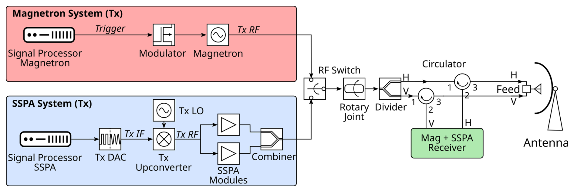
Figure 1 Block diagram of the main parts of the transmitter chain of the upgraded DWSR5001 with switchable magnetron and SSPA.

Implementing fast transmitter switching required several modifications throughout the system. Because the radar employs a receiver-over-elevation configuration with the transmitters located in an equipment room below the radome, changes were necessary in both the transmitter and receiver subsystems. The original magnetron transmitter remained unchanged. The SSPA was integrated by installing an additional cabinet adjacent to the two existing transmitter racks. This cabinet houses the SSPA assembly manufactured by RFHIC along with a second signal processor, a transmit digital-to-analog converter (Tx DAC), an upconverter, and a coaxial switch box (the latter not shown in the schematic in Fig. 1). The SSPA system itself consists of three rack-mounted units: one unit containing power supply, control, and status electronics, and two identical amplifier units that include the driver and radio frequency (RF) stages.

The overall transmitter configuration is shown in Fig. 1. The signal generation in the SSPA system differs fundamentally from that of the magnetron. Instead of triggering a high-voltage modulator, the SSPA uses predefined digitally modulated bursts. These digital waveforms are converted to an analog intermediate-frequency (IF) signal at 60 MHz using the Tx DAC. Upconversion to the final transmit frequency of 5640 MHz is achieved by mixing the IF signal with a local oscillator (LO). The resulting RF signal is then split equally and fed into the two SSPA amplifier modules. Driver stages provide the required input levels for the subsequent high-power GaN amplifier (HPA) stages, which operate in saturation for maximum efficiency and therefore exhibit strong non-linearity. Each amplifier unit contains four HPA modules, each delivering approximately 1.2 kW. The outputs are combined in a two-stage combiner to produce a total peak power of about 10 kW – substantially lower than the 500 kW peak power of the magnetron transmitter.

The outputs of the magnetron and SSPA transmitters are routed into a waveguide switch controlled by the radar control unit (RCU), which selects the active transmitter. Downstream of the switch, both systems share the same hardware: rotary joints, the horizontal/vertical (H/V) power divider, and the antenna. In this radar design, H- and V-polarized signals must be generated via waveguide splitting rather than via separate transmitter chains, as used in some other implementations with independent H- and V-channel amplifiers that support distinct pulse shapes (e.g. Schneebeli et al., 2025).

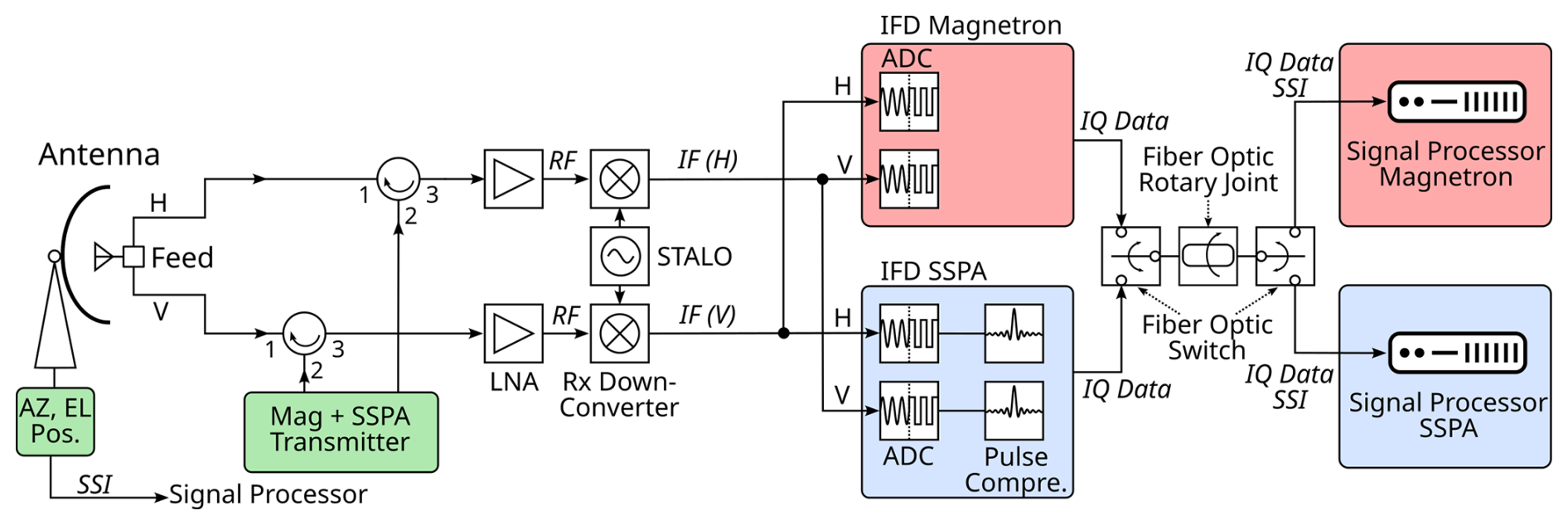
Figure 2 Block diagram of the main parts of the receiver chain of the upgraded DWSR5001 with dual digital receiver and signal processors for alternating SSPA and magnetron use.

The receiver configuration is illustrated in Fig. 2. The analog receiver front-end, located in a cabinet behind the antenna, is shared by both transmitters down to the IF stage. A splitter is added in the IF path to integrate a second intermediate-frequency digitizer (IFD) dedicated to SSPA reception. An independent IFD is required because pulse compression is performed directly in the IFD. The digitized I&Q data are sent via fiber-optic link to the respective signal processors in the equipment room. Additional switches ensure that the active IFD and signal processor receive the correct signals, including azimuth (AZ) and elevation (EL) angle information provided through synchronous serial interface (SSI), which also needs to be routed to the appropriate processor. The signal processor then applies configurable processing steps to generate the standard radar moments.

During the SSPA tests, a transmission scheme consisting of a 97 µs nonlinear frequency-modulated (NLFM) long pulse followed immediately by a 1.3 µs un-modulated short pulse was used. The two pulses are transmitted at center frequencies separated by 6.1 MHz, allowing simultaneous reception and processing and thereby optimizing scan time. The NLFM long pulse has a bandwidth of 2.8 MHz, achieving a peak sidelobe level (PSL) of −60 dB and an integrated sidelobe level (ISL) of about −55 dB. These values are reached by using a tapered and mismatched version of the transmitted pulse for the cross-correlation with the received pulse. After compression, the effective range resolution is 130 m, with the IFD oversampling the compressed pulse at approximately 30 m resolution. The theoretical time-bandwidth compression gain is 24.3 dB, while the effective gain is 15.9 dB, reduced by filter losses, receiver noise, and pulse-shaping effects.

Calibration of the long pulse data is performed by adjusting the compressed-power values within a range interval where both long and short pulse data overlap. This is done independently for the H- and V-channels. A similar correction is applied to the differential phase PhiDP to ensure continuity across the transition from long to short pulse data.

2.2 Scan strategy and configuration

All of the data shown here have been acquired by running a scanning scheme close to the one used in the operational DWD radar network. One such operational scan cycle takes 5 min and consists of six distinct scans:

• a terrain following precipitation scan, where the elevation is adapted as a function of azimuth. This scan is used to gather near-ground precipitation information.

• a volume scan consisting of 10 sweeps at fixed elevations (from 0.5 to 25°). The purpose is to gather three dimensional information of precipitation with a high Nyquist interval for the Doppler measurement.

• a 90° elevation birdbath scan, used mostly for calibration of the differential reflectivity (ZDR), but more recently for microphysical investigations as well (Gergely et al., 2022).

• a fixed clutter target scan used to monitor the coherency of the radar system

• a calibration scan to perform a one-point calibration using an internal test signal generator (ITSG)

• a fixed angle scan pointing North at the end of each scan cycle. This guarantees that all radars in the network start from the same azimuth position to minimize radar-radar induced interferences (Frech et al., 2023).

Further details about DWD's operational scanning scheme can be found in Seltmann et al. (2013). The MOHP dual transmitter radar has been setup to alternate between both transmitters; the magnetron system begins the cycle every full 10 min (minutes 00, 10, 20, …). After 5 min, it hands over control to the SSPA, which then completes the same five minute cycle and returns control to MAG.

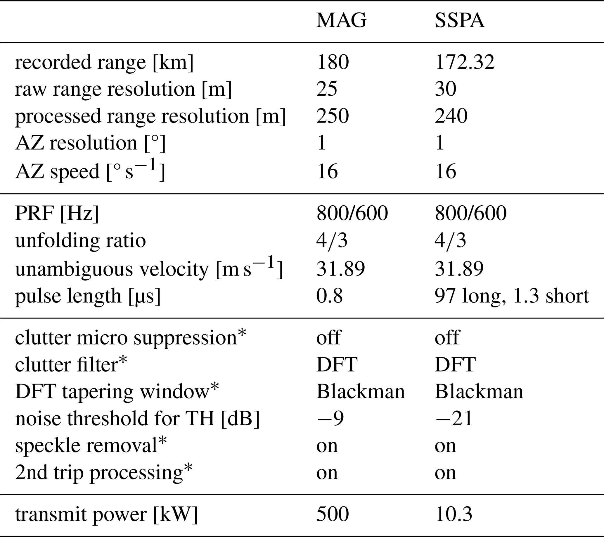
The settings for the sweep recorded at 1.5° EL, which is used throughout the paper, is detailed in Table 1. There are only few differences in the setup between MAG and SSPA: Lower transmit power requires a longer pulse in SSPA, which in turn decreases the unambiguous range. The difference in raw range bin resolution (25 m vs. 30 m) is a design choice by the manufacturer that leads to a slight difference in the processed range bin resolution of 250 and 240 m, respectively. Other sweeps require more adaptions to SSPA: The lower transmit power of SSPA presupposes considerably longer pulses, increasing the duty cycle to a level which can only be compensated by decreasing the PRF. Subsequently, the rotational speed of the antenna might have to be decreased to collect an amount of samples that is enough for a meaningful Fourier transform. Depending on the required range coverage and unambiguous velocity range, PRF staggering ratios also have to be adjusted.

Table 1 Settings of the 1.5° EL radar scan used in the evaluation. Settings marked with ^∗ only apply to the corrected processing chain.

This dual-transmitter setup results in data where differences can be directly attributed to the transmitter type and the five minute offset in measurement time.

3 Results

This section details the results of the dual transmitter setup at MOHP. Similarities and differences in the observed data quality of the two systems are analyzed.

The goal of the switching dual-transmitter test is to evaluate if SSPA technology can be used as a viable substitution for the current magnetron transmitter. To be viable, the SSPA radar is required to yield at least comparable data quality and sensitivity with respect to the magnetron system. The following sections contain a detailed view on sensitivity and reflectivity, Doppler moments and dual-polarization data. In addition, Sect. 3.5 and 3.6 highlight unique properties of the SSPA data originating from the chosen pulse train and pulse compression. For this study, we fully rely on radar data that have not gone through any filtering by the signal processor, identifiable by the leading “U” (uncorrected) in the moment names. This includes, e.g., clutter removal, 2nd-trip processing and speckle filtering, which are enabled for the simultaneously generated corrected processing chain.

3.1 Examples from a stratiform and a convective event

The data from two distinct meteorological situations are the basis for all shown assessments and will be further evaluated in depth in the following sections for multiple radar moments. They are characterized in the following paragraphs.

To identify areas containing precipitation, we solely use a co-polar cross-correlation coefficient (RhoHV) threshold of 0.6 for both the SSPA and MAG data. This value is arbitrarily chosen, but performs well to remove most non-meteorological echoes and measurements close to the noise level. Strong clutter signals from the Alps south of the radar remain, but they pose a viable element to investigate. For more details on RhoHV see Sect. 3.4. The PPI images in Figs. 3 and 4 additionally use the noise thresholds detailed in Table 1.

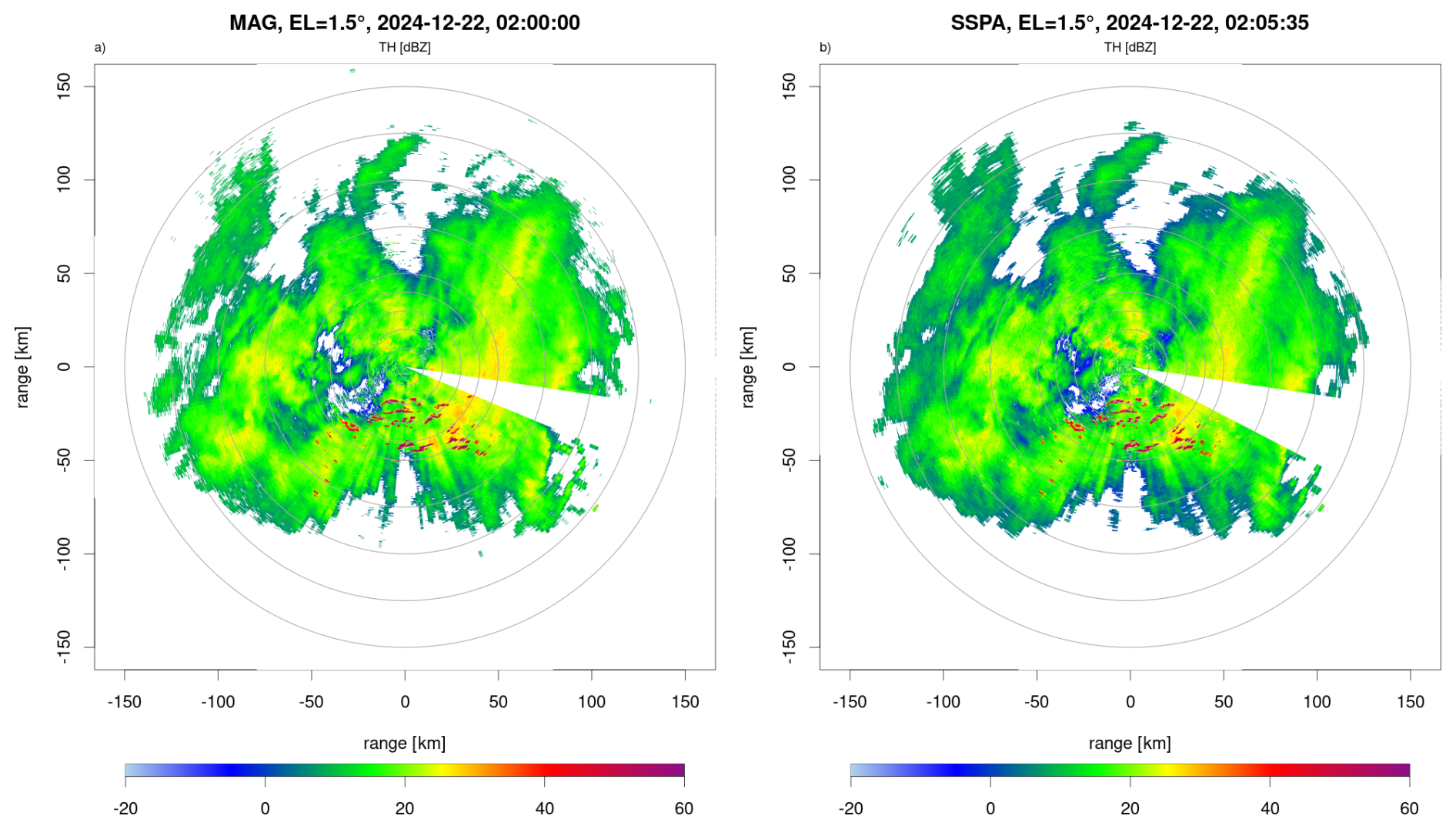
Figure 3 PPI images of the uncorrected reflectivity (TH) from a scan in 1.5° elevation from (a) MAG and (b) SSPA. Data were recorded during a stratiform event in December 2024. Both are thresholded with RhoHV, where everything below 0.6 is removed. Data points exceeding 50 dBZ are the Alps. The grey rings mark the distance from the radar in 10 km spacing between 0 and 50 km and 25 km further out.

The first event was recorded over 13 h in December 2024 during stratiform precipitation. The data set consists of 72 sweeps from MAG and SSPA each at an elevation of 1.5°. Figure 3 shows two corresponding PPIs of the uncorrected reflectivity (TH) for MAG and SSPA from one time step during this winter snow fall event. Because of a public area within the safety distance of the radar, a safe sector blanking is implemented in an azimuth between 100–112° (MAG) and 100–117° (SSPA). Transmitters are turned off within this sector. Clutter free maximum radar reflectivity in precipitation reaches 30 dBZ. Strong clutter signals south of the radar (with TH of up to 60 dBZ) originate from mountains in both MAG and SSPA data. The spatial variability and extent of precipitation is very similar between MAG and SSPA. However, there are distinct differences at ranges larger than 100 km. For example the reflectivity in the Northwest is spatially smoother and larger in size for the SSPA. A detailed discussion regarding the sensitivity and reflectivity follows in Sect. 3.2.

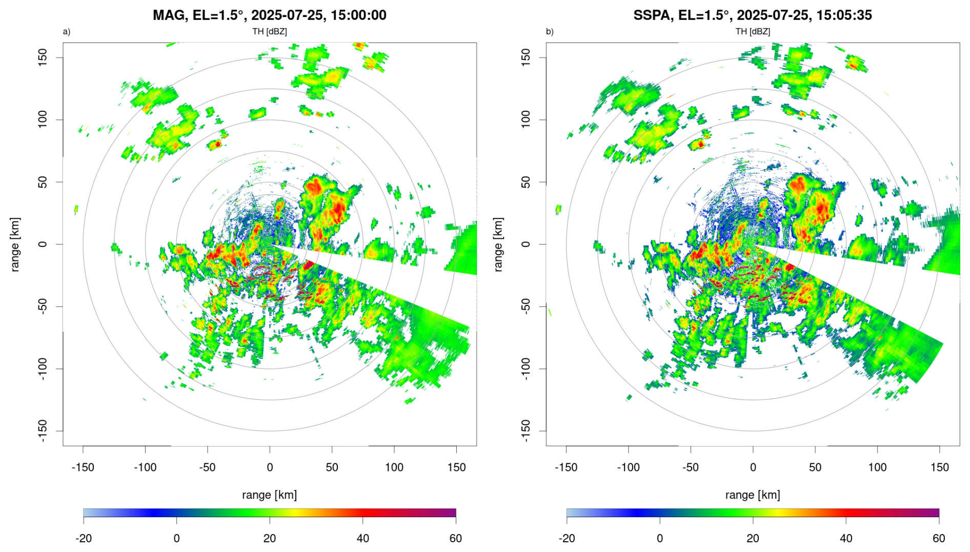
Figure 4 PPI images of the uncorrected reflectivity (TH) from a scan in 1.5° elevation from (a) MAG and (b) SSPA. Data were recorded during a convective event in July 2025. Both are thresholded with RhoHV, where everything below 0.6 is removed. See also Fig. 3.

The other data set contains a convective event, during which we collected 52 sweeps per transmitter over 9 h total in July 2025. Here we also select the 1.5° elevation sweep, as this sweep has low ground clutter contamination near the radar. Figure 4 shows TH for this convective precipitation event. While the general direction of movement of the precipitation was from the South, the convective cells were generated locally and showed no preferential direction. Additional details can be found in Sect. 3.3, where Doppler velocities are discussed. Recorded reflectivities with both transmitters range between 50 and 60 dBZ in the convective cells. Both show good agreement in strength and location, at least in the inner 75 km range. The structure and area of the convective cells do not show significant differences, indicating that the chosen pulse length and frequency modulation lead to comparable spatial resolution. Further away from the radar, convective cores at the edge of the recorded range appear more spatially smooth and defined in the SSPA data. At the location with clutter from the mountains we note range sidelobes with enhanced reflectivity values in radial direction. These are further discussed in Sect. 3.6. Additional details regarding the meteorological situation are given with the other radar moments in the following sections.

3.2 Sensitivity and reflectivity

The radar reflectivity Z is the most important quantity measured by a weather radar. It is commonly used to estimate a corresponding precipitation rate via empirical $Z/R$ relationships.

Sensitivity describes the smallest signal that is still detectable by the radar at a given range. If a radar has a high sensitivity, even small rainrates can be detected at a larger range. The sensitivity of a radar is determined by the smallest power still measurable by the receiver, usually given in dBm. Together with the calibration factor dBZ₀, a range dependent minimum detectable reflectivity can be determined. dBZ₀ is measured during radar calibration for each transmitter and polarization. By applying a range factor and the frequency dependent gas attenuation, the range dependency of dBZ₀ for the horizontal channel can be described as:

$$\begin{array}{}\text{(1)}& {\mathrm{dBZ}}_{\mathrm{0},r}h={\mathrm{dBZ}}_{\mathrm{0}}h+\mathrm{20}\cdot {\log }_{\mathrm{10}}\left(r\right)+A_{\mathrm{gas}}*r\end{array}$$

where r is the range in km, A_gas the two-way gas attenuation in dB km⁻¹ (0.016 for C-Band, valid at low elevations) and dBZ₀h the minimum detectable signal of the horizontal channel in dBZ at 1 km distance to the radar. For DWD's MOHP magnetron radar, dBZ₀h is −38.31 dBZ. More transmit power translates to a higher sensitivity. For the SSPA, absolute calibration is done using the short pulse (see Sect. 2.1). Since the transmit power is smaller (10.2 kW), the resulting sensitivity of an un-modulated pulse with a duration similar to the typical magnetron pulse is much lower. In our case we get a dBZ₀h of −29.86 dBZ for the SSPA. However, this difference in sensitivity is compensated by the additional gain from pulse compression in the modulated long pulse of the SSPA. The NLFM of the long pulse not only provides a range resolution comparable to the MAG, but also increases sensitivity by the pulse compression gain. In our case, we get an effective pulse compression gain of 15.9 dB for the pulse form in use. This results in a theoretical dBZ₀h of −45.76 dBZ for the SSPA long pulse and therefore a higher sensitivity compared to the MAG.

To statistically verify the effective pulse compression gain from our data, we use uncorrected radar reflectivity data TH from the stratiform rain event described in Sect. 3.1. To simplify the evaluation, we threshold the data with RhoHV < 0.6 in order to remove most non-meteorological signals, without introducing algorithmic complexity to the interpretation of the results. An additional noise threshold (see Table 1) is applied during signal processing. The remaining radar pixels are binned by reflectivity (0.5 dBZ step) and range (1000 m step) to form a 3d histogram. To account for the differences in range resolution (see Sect. 2.2), resulting counts are normalized by the amount of range gates represented by each histogram bin.

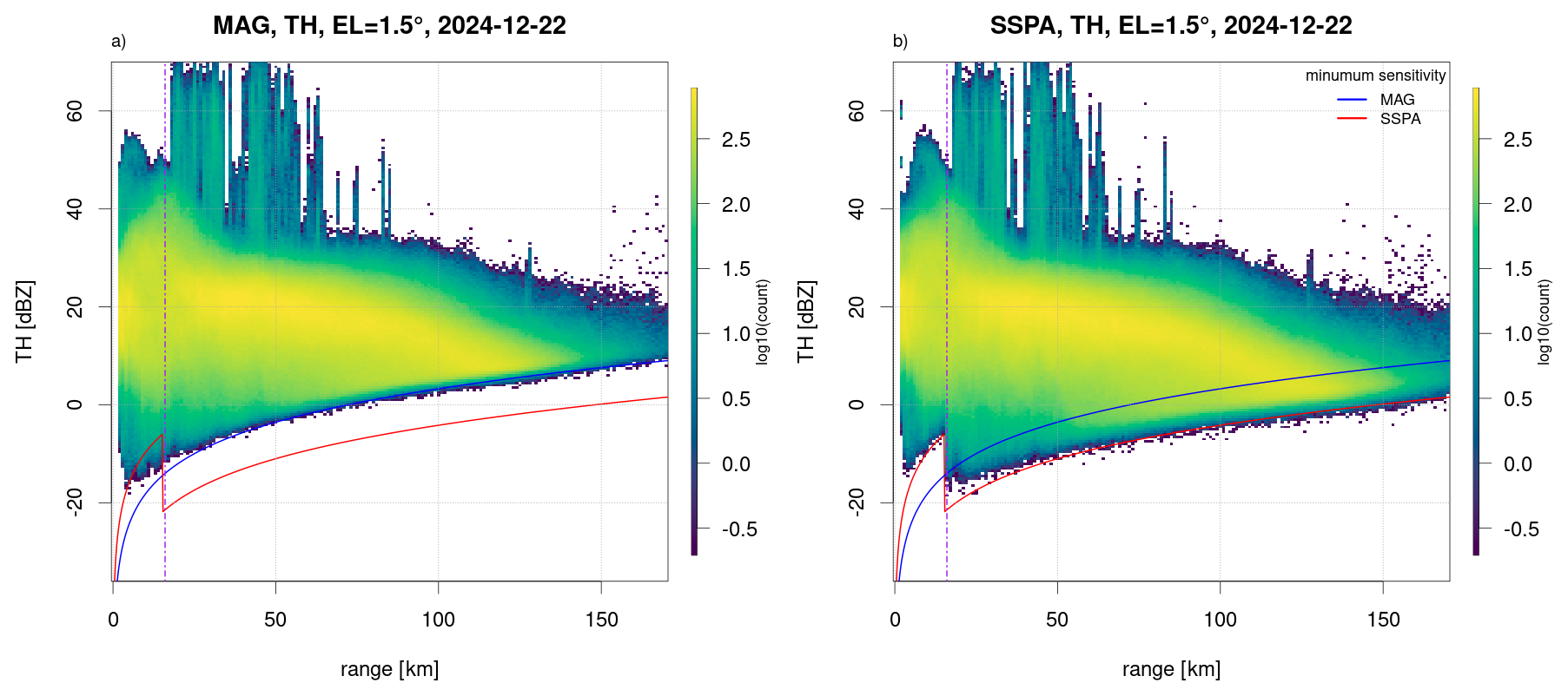
Figure 5 Frequency of reflectivity values in dependence on range, from 1.5° elevation and (a) MAG and (b) SSPA. Data thresholded with RhoHV < 0.6 and aggregated over 13 h (72 sweeps per transmitter). Blue and red lines show the calculated minimum sensitivity for MAG and SSPA respectively. The vertical purple dashed line marks the short pulse/long pulse border. Logarithmic histogram counts are shown as colors.

Figure 5 shows the number of radar pixels for MAG and SSPA falling into each histogram bin in logarithmic counts in color scale. The red and blue lines represent the expected sensitivity using Eq. (1), applying the values obtained from calibration. For MAG in Fig. 5a, the actual recorded weather data closely follows the expected sensitivity line shown in blue. Nearly all remaining radar pixels after thresholding stay above the minimal detectable precipitation signal line. With SSPA, the red line follows the data in the inner 16 km, up to the vertical purple dashed line that marks the border between the short and long pulse. This is to be expected, since only the short pulse can be calibrated. In the area of the long pulse, the recorded data shows substantially lower values than what would be expected by extrapolating the sensitivity determined in the short pulse. This is the effect of the pulse compression gain, which averages to 16.8 dB in the presented case. This slightly depends on the selected RhoHV threshold, but aligns with the theoretical gain (15.9 dB) and also clearly exceeds the difference of about 9 dB to the overall magnetron sensitivity value. Thus, the SSPA system, with the presented transmit power and the employed pulse compression, shows better sensitivity (7 dB) in the long pulse region. At the same time, lower sensitivity of the SSPA in the short pulse region up to 16 km is found.

The general distribution of the data, shown as colors, is similar. Maximum values per range reach comparable levels. The maximum values, measured in clutter, appear at the same locations. With both transmitters, the bulk of the measurements are between 0 and 40 dBZ close to the radar, where clutter plays a major role. At greater distances, precipitation causes a signal of, on average, 20 dBZ, which is decreasing with increasing range.

Only the long pulse profits from compression gain. The short pulse does have a lower sensitivity than MAG. With the previously mentioned dBZ₀ of the SSPA of −29.86 dBZ, the minimum detectable reflectivity at a range of 16 km is −5.6 dBZ. Using the default Z–R-relationship of DWD (Aniol et al., 1980), this reflectivity corresponds to a rain rate of 0.008 mm h⁻¹. The reduced sensitivity in the short pulse range may therefore be relevant for climatological application using radar data. The relevance for e.g. meteorological nowcasting applications still needs to be assessed.

However, it is important to note that this difference is only caused by missing light precipitation, not by incorrect measurements of precipitation above the minimal detectable signal level. The limitations of a 2-pulse scheme are expected to be mitigated in the future by new processing techniques which use the long pulse returns in the range < 16 km (Malkomes, 2025). First experiments with this approach have been conducted with the presented radar setup, but require more detailed analysis.

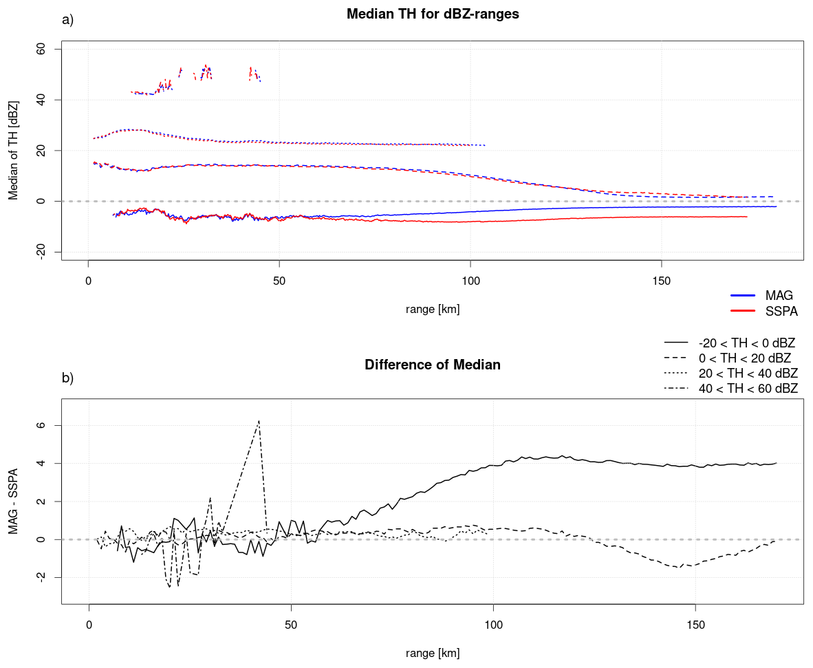
Figure 6 (a) Median TH for four classes of recorded reflectivity. (b) Difference in the median of the four classes. Differences were calculated from interpolated data on 1 km range resolution. Data taken from all AZ angles over 72 sweeps with an elevation of 1.5° per transmitter during the 2024 stratiform event. Data points are removed if the sample is smaller than 750 values.

Figure 7 Amount of valid data points per reflectivity category and transmitter during the 2024 stratiform event. These values are valid for Figs. 6, 10, 13, 14 and 16.

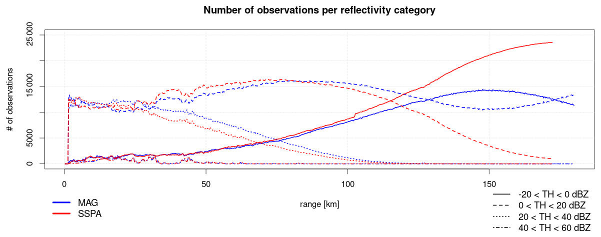
Figure 6 shows the data from the same precipitation event, but without any thresholding (Noise or RhoHV). Data over all azimuth angles and time steps are collected and binned into four reflectivity categories. For each category and range, the median is calculated. Differences in median in Fig. 6b are determined from values interpolated to 1 km range spacing to overcome the difference in range resolution. The highest class ranging from 40 to 60 dBZ contains only clutter pixels, their total number over the whole period does not exceed 2000 samples in any range (cf. Fig. 7). Still, both transmitters agree well in the measured values. Most of the precipitation falls into the two middle categories from 0 to 40 dBZ with up to 15 000 samples per range. Within those two classes, both transmitters agree well up to a range of about 130 km. As can be seen in Fig. 6b, the differences of the median values (MAG–SSPA) are below 1 dBZ. Beyond 130 km (for values of TH between 0 and 20 dBZ), SSPA median values are slightly larger by up to 1.7 dBZ. This relates to the increased sensitivity of the radar system with the SSPA transmitter. SSPA still has valid measurements, while the MAG measurements converge to noise more quickly. The lowest class between −20 and 0 dBZ contains precipitation only to a range of approximately 60 km, but the sample size per range is again below 2000. Up to this range, median values show good agreement. At larger ranges, the sensitivity of both systems is too low to measure weak precipitation. The data here therefore contain only noise and converges towards the values in the lowest category. SSPA medians in no class show any distinct jump in the data at 16 km, where short and long pulse are matched.

This evaluation indicates that both transmitter types measure very comparable reflectivity values over the typical range of −20 to 60 dBZ. At large distances from the radar and with weak precipitation, the sensitivity advantage of the SSPA due to pulse compression becomes apparent. We were able to confirm these findings with the data from the convective event, and for TV from the vertical channel as well.

3.3 Doppler moments

To get reliable Doppler information, the DWD radars are required to resolve velocities up to ±32 m s⁻¹ in the volume scan (see Sect. 2.2). To reach this value, and to cover a range of up to 180 km, both transmitters use a staggered PRF of 800/600 Hz and a $\mathrm{4}/\mathrm{3}$ Doppler unfolding ratio for the 1.5° elevation scan. Figure 8 shows the uncorrected, unfolded Doppler velocity (UVRADH) as PPI for the same date and time as Fig. 3 for reflectivity. No noise or RhoHV thresholding is applied to the UVRADH data.

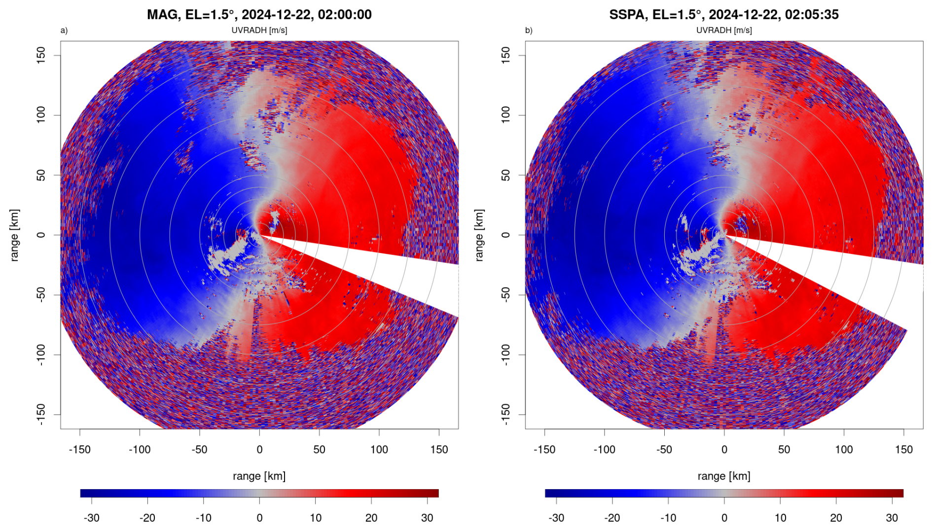
Figure 8 PPI images of the uncorrected and unfolded radial velocity (UVRADH) from a scan in 1.5° elevation from (a) MAG and (b) SSPA. Data were recorded during a stratiform event in December 2024. No thresholding was applied. See also Fig. 3.

Both transmitters show an increasing noise at the edges of the precipitation areas where the signal strength is falling off. Additionally, velocities south of the radar at a range of about 50 km are contaminated by clutter caused by the Alps. Overall, the SSPA appears to be able to recover more valid measurements, especially at a larger range, leading to more spatially homogeneous and smooth data. Particularly in the Northwest of the radar, at ranges larger than 150 km, the SSPA shows a better coverage with valid Doppler data, a consequence of the higher sensitivity of the SSPA system in the long pulse range.

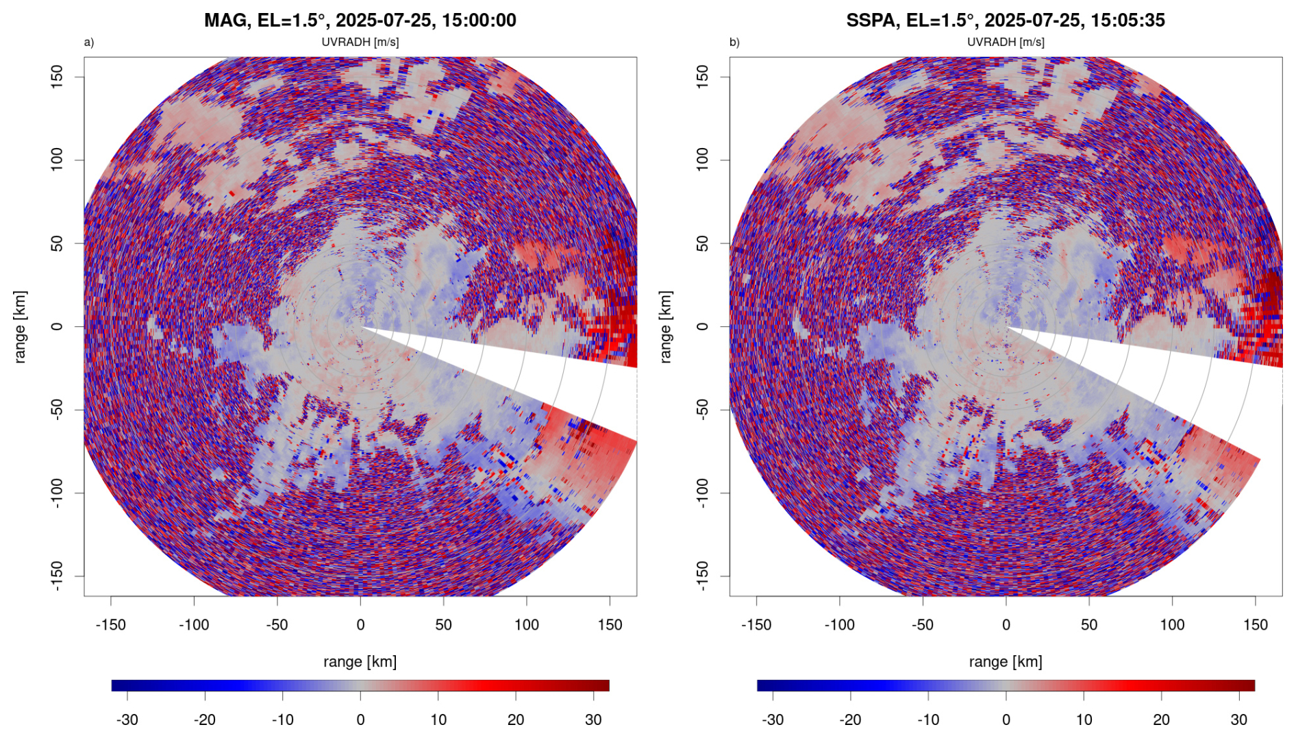
Figure 9 PPI images of the uncorrected and unfolded radial velocity (UVRADH) from a scan in 1.5° elevation from (a) MAG and (b) SSPA. Data were recorded during a convective event in July 2025. No thresholding was applied. See also Fig. 3.

The Doppler velocities for the convective event in Fig. 9 show the quasi-stationary nature of the thunderstorms. Absolute velocities are below 10 m s⁻¹ and no preferential direction is apparent. Within the inner 75 km, both radars show a good agreement, both in speed and direction. An interesting feature seen by both transmitters is the area of divergence in the southeast, just south of the blanked sector at 125 km range. Here we also see more noisy measurements, caused by the low signal strength. More of these are apparent in MAG data than in SSPA, again showing the advantage of SSPA when the returned signal is weak.

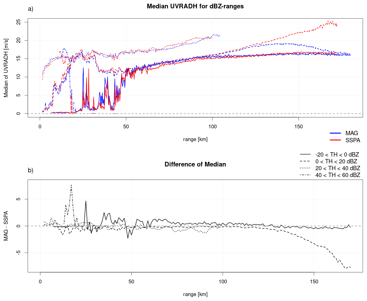
Figure 10 (a) Median radial velocity (UVRADH) for four classes of recorded reflectivity. (b) Difference in the median of the four classes. Differences were calculated from interpolated data on 1 km range resolution. Data taken from all AZ angles over 92 sweeps with an elevation of 1.5° for each transmitter. Data points are removed if the sample is smaller than 750 values.

Following the same processing as for the reflectivity in Fig. 6, we present the same image for the recorded Doppler velocities in Fig. 10. Data are again taken from the stratiform event in 2024. No thresholding was applied, but all values were converted to their absolutes to achieve independence from the azimuth angle. The bulk of all measurements shows an average Doppler velocity over all reflectivity categories of about 15 m s⁻¹. The range at which this velocity occurs varies, and depends on the respective reflectivity class. The highest category with a TH between 40 and 60 dBZ occurs – as described above – almost only in clutter and has a low amount of samples. The velocity here accordingly converges towards 0 m s⁻¹. Most Doppler measurements close to the radar (the inner 50 km) fall between 20 and 40 dBZ (cf. Fig. 7). The corresponding velocity starts at 10 m s⁻¹, and increases with range, following the expected increase of wind speed at higher altitude. Measurements with TH between 0 and 20 dBZ start at 0 m s⁻¹ and might therefore contain weak clutter. At a range of about 20 km, velocities in this category reach the same values as the previous category. They then experience a small reduction which is visible with both transmitters, until they start to linearly increase at about 60 km. The lowest reflectivity category with values between −20 and 0 dBZ contains mostly noise outside a range of 60 km, yet the data from both transmitters agrees well also closer to the radar, where valid measurements are present.

Over all, the Doppler data from MAG and SSPA show very good agreement over all TH categories up to a range of 130 km. At larger ranges, most valid measurements lie in a reflectivity range between 0 and 20 dBZ. As was already described above, MAG values in this range approach the magnitudes found in the lowest reflectivity category, which at that range contains only noise. The median velocity in noise converges towards 17 m s⁻¹. SSPA data show the expected velocity increase out to almost the maximum recorded range. This can be seen in Fig. 10b, where the difference in median increases only for the dashed line (Doppler data in the TH range 0 and 20 dBZ). These findings support the impression from the PPIs that SSPA can record valid velocity measurements up to a larger range than MAG. Same results are found for the Doppler data from the vertical channel. The convective event was not evaluated in detail, because the low Doppler velocities and varying wind directions prevent a conclusive interpretation.

3.4 Dual-polarization moments

Dual-polarization moments are derived from the horizontal and vertical polarization data of the radar measurement. In the following we discuss differences in the cross correlation coefficient RhoHV, differential phase PhiDP and the differential reflectivity ZDR.

The cross correlation coefficient RhoHV is often used to distinguish between signals of meteorological and non-meteorological origin. Stratiform and liquid precipitation RhoHV values are expected to be close to 1.0. The value can drop to about 0.7 in snow and hail. RhoHV values of 0.6 and below are usually not related to precipitation, although there are reports of RhoHV values as low as 0.3 for very large hail (Ryzhkov and Zrnic, 2019).

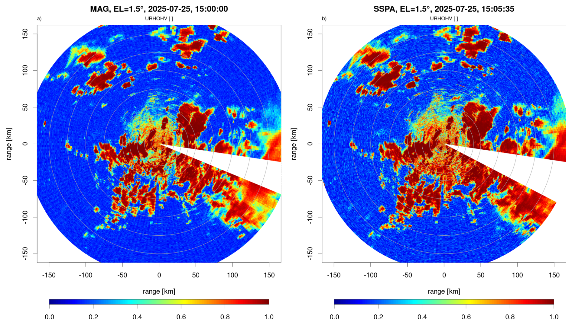
Figure 11 PPI images of the uncorrected correlation coefficient (URHOHV) from a scan in 1.5° elevation from (a) MAG and (b) SSPA during the convective event. See also Fig. 3.

Being able to measure a high RhoHV (> 0.99) in suitable precipitation is a measure of quality for a dual-polarization weather radar. Both transmitters are able to measure a high RhoHV in convective cores, as shown in Fig. 11. Due to the high values, we can assume that no hail was present in the thunderstorms recorded during that time. Substantial differences are again apparent in the range-time sidelobes caused by the pulse compression directly to the south (AZ 160–200°, 30–60 km range) that also modify the dual-polarization characteristics (see Sect. 3.6). At larger ranges, differences are apparent, where the SSPA is able to measure high RhoHV even at the maximum recorded range, where the strength of the received signal is low. MAG RhoHV gradually deteriorates with increasing range due to decreasing SNR, and values close to 1 can only be measured in the center of the strongest convective cores.

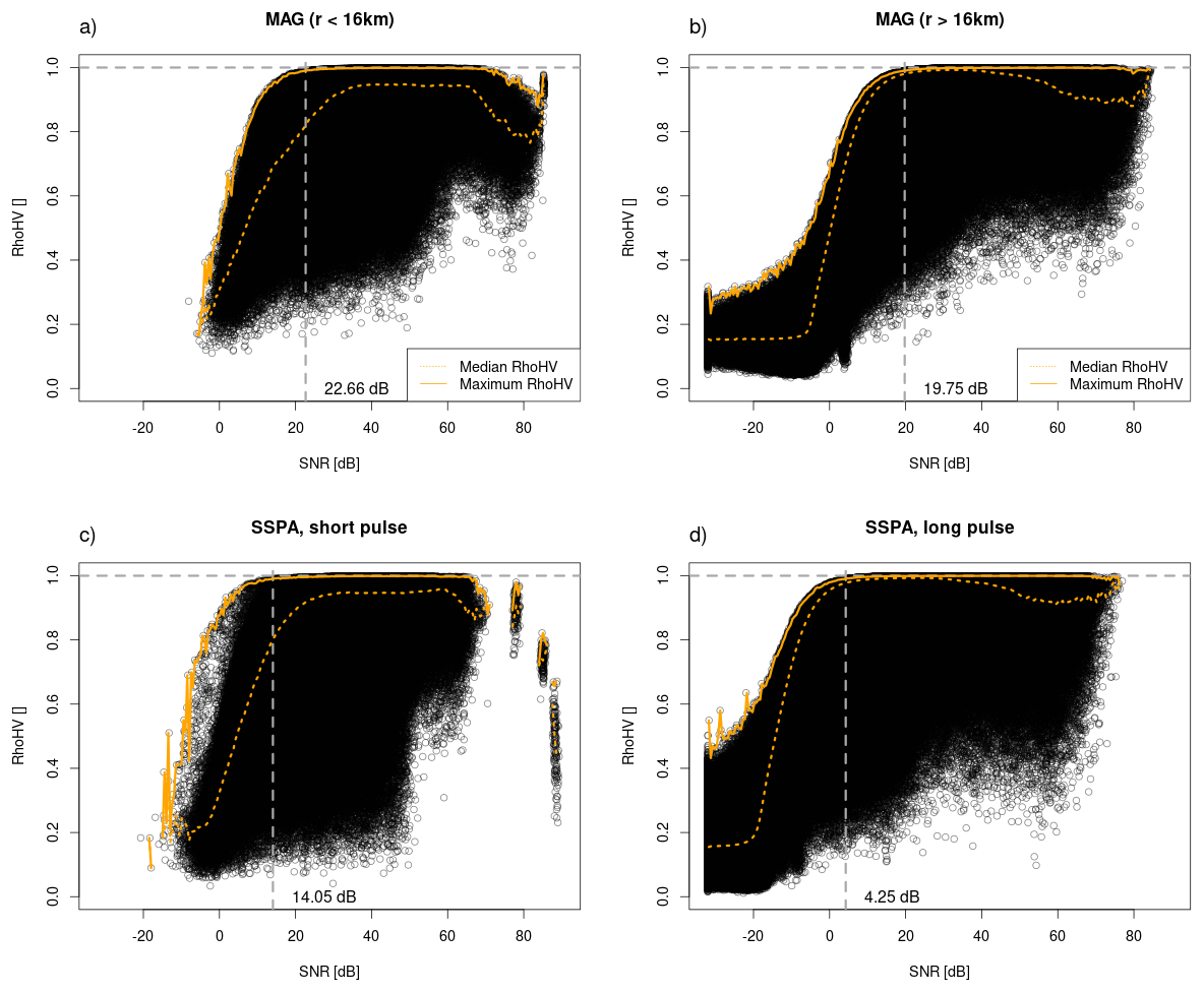
Figure 12 Relationship between the measured SNR and RhoHV for (a) MAG in the inner 16 km, (b) MAG in the range > 16 km, (c) SSPA short pulse and (d) SSPA long pulse. Data recorded during the stratiform event in December 2024. Orange solid and dashed lines are the maximum and median RhoHV, respectively. The horizontal grey line is a RhoHV of 0.99, and the vertical grey line shows at which SNR this RhoHV is first reached. The exact value is written at the bottom of each panel.

A simple visual inspection of the data confirms that both transmitters presented here are able to measure a RhoHV of close to one. However, the performance of a radar can be analysed further, based on additional factors needed to reach a specific RhoHV level. There is a very clear dependency of RhoHV on the signal-to-noise ratio (SNR), as it is shown in Fig. 12, where all RhoHV values recorded during the stratiform event in 2024 are plotted against their respective SNR (horizontal channel only). In all cases, high RhoHV values are only reached after surpassing a sufficient SNR level. This can be mitigated using the noise correction suggested in Ryzhkov and Zrnic (2019), but was not done for this data. The lowest SNR at which RhoHV equal to 0.99 is reached is written at the bottom of each panel and indicated by the vertical grey line. For MAG beyond the 16 km range (Fig. 12b), a RhoHV of 0.99 is first reached at a SNR of 19.75 dB and is constantly lower for lower SNR. This matches the numbers found in Ryzhkov and Zrnic (2019).

Closer to the radar (Fig. 12a), a higher SNR of 22.7 dB is required for MAG compared to ranges further away.

The reason lies in the way the noise sample is measured in the radar. It is taken while the transmitter is turned off and the antenna is pointing vertically upwards. Therefore, very little ambient thermal radiation from the ground will enter the system. For the data that is shown here and taken from the 1.5° EL scan, the actual noise is higher, because the antenna main lobe intersects with the ground and will pick up the emitted radiation, which is then added to the internal system noise. At a range above 16 km, less intersection with the ground occurs and the noise sample taken at 90° EL is more representative.

The short pulse of the SSPA in Fig. 12c is expected to behave similar to the MAG pulse, because it is an un-modulated pulse. With it, the system reaches RhoHV > 0.99 with an SNR of least 14.05 dB, which is substantially lower than for MAG. We attribute this to a much lower noise power (≈ 3 dB higher for MAG than for SSPA). This is caused by the smaller bandwidth of the SSPA short pulse and its much narrower matched filter, which is required to separate the return of long and short pulses during simultaneous receiving.

Theoretically, a RhoHV of > 0.99 in the modulated long pulse would then be expected at 14.05 dB from the short pulse minus the compression gain of 15.9 dB, resulting in an SNR of −1.85 dB. The actual number is much higher with 4.25 dB (cf. Fig. 12d).

Values calculated during the convective event are almost identical, so the described effect does not depend on precipitation type.

It must be noted that absolute SNR values can not be compared easily between MAG and SSPA. They represent the ratio between noise and signal, but for SSPA, the determined compression gain is added to the signal strength before the calculation of SNR. Additional differences come from the noise estimation, the transmit power and the pulse length that determines the integration time for the calculation.

The orange lines in Fig. 12 are the maximum and median RhoHV per SNR. Where these two lines appear to overlap, the radar recorded clutter free, homogeneous precipitation. This is only the case outside of 16 km, because at closer ranges, data are more heavily influenced by ground clutter. In MAG data, these conditions occur in a SNR range between 20 and 40 dB. For SSPA, the span is larger and ranges from 5 to 40 dB. This shows that SSPA has a larger range in which high RhoHV can be measured. It is not just shifted towards lower SNR. The median RhoHV drops at higher SNR due to the presence of clutter (Fig. 12).

Overall, this implies that SSPA has better sensitivity in the pulse compressed region, leading to higher RhoHV in weak precipitation, at the edges of precipitation areas and also at a larger range compared to MAG.

Let us revisit the the PPI of RhoHV in Fig. 11. Both transmitters reach a high value within homogeneous precipitation. The advantage of the SSPA becomes clear at the edges: While in MAG data, the gradient area between high and low values is clearly present (displayed in green and yellow), it is much more defined in SSPA data. Lower SNR is sufficient for SSPA to measure a high RhoHV, while this is not sufficient for MAG. These effects can be seen under stratiform conditions as well (not shown).

Figure 13 Like Fig. 10, but for the uncorrected correlation coefficient RhoHV.

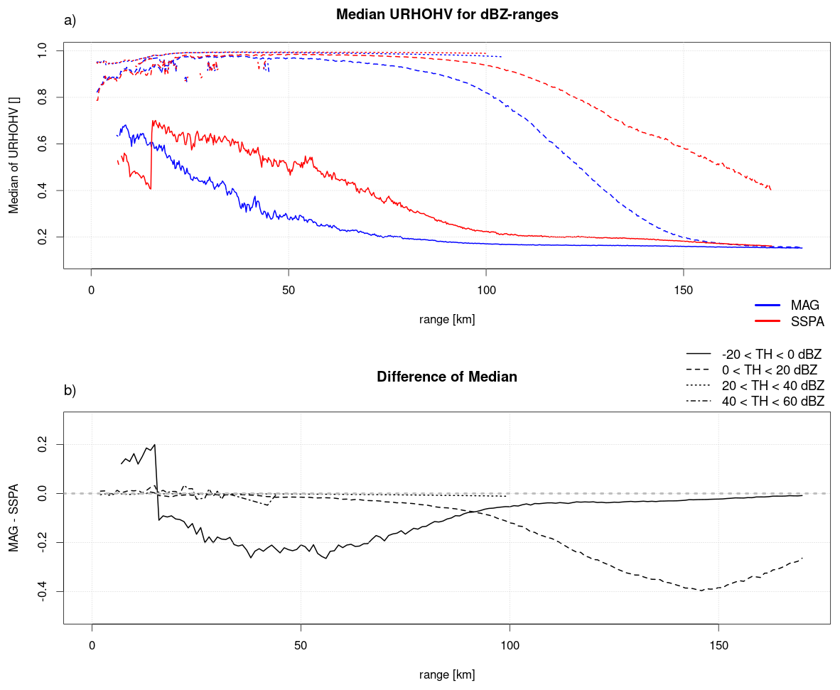
Figure 13 shows the range dependence of RhoHV for the stratiform case, again grouped into four categories of TH. Data shown here are uncorrected (no threshold applied). Values that fall into the three highest TH categories (0 to 60 dBZ) match very well up to a range of about 50 km from the radar. While RhoHV stays high for both transmitters at larger ranges when the reflectivity is greater than 20 dBZ, the median clearly drops in MAG data for the category 0 to 20 dBZ. SSPA RhoHV stays above 0.9 to about 100 km. These reflectivities are measured in areas with low SNR, so this figure confirms the findings from the comparison of RhoHV with SNR, but now with the consideration of the range dependency of SNR.

RhoHV data from the lowest TH category (−20 to 0 dBZ) shows an interesting feature: The median for the SSPA has a distinct jump at a range of about 16 km where short and long pulse are matched. Within the short pulse range, RhoHV has a lower value than MAG and drops to even lower values. This is due to the decrease of SNR with increasing range. With the start of the long pulse, RhoHV shows a sharp increase because the pulse compression is able to raise SNR to the necessary level. As described above, this reflectivity category contains less and less valid measurements with increasing range due to the decreasing sensitivity and consists therefore of mostly noise, so the higher RhoHV in SSPA measurements (about 0.7) can not be attributed to precipitation, but to the higher coherency of the system, which allows for higher RhoHV even in noise. With the presented categorization into four classes, the jump is only visible in the lowest reflectivity category. Further investigation shows that we find a reduction of the maximum RhoHV in the category from 0 to 20 dBZ down to 0.995 in the short pulse region. When limiting the category to a span from 0 to 10 dBZ, the maximum RhoHV drops to 0.97. This matches the results from Fig. 12. Using the SNR limit from there, a minimum reflectivity value of 8.1 dBZ is required at the end of the short pulse to achieve a RhoHV of 0.99 or higher. The performance in the short pulse might therefore be only sufficient for precipitation exceeding 10 dBZ. In cases with weaker signals, short pulse data lacks in quality.

Data from the convective case looks very similar, with the difference that the median RhoHV in the category between 0 and 20 dBZ is lower. We attribute this to the convective nature of the event: Most cells contain strong precipitation, so that they fall into the higher categories. The category from 0 to 20 dBZ therefore consists of more range gates with clutter, where RhoHV is lower than in precipitation.

Another important dual-polarization moment is the difference of the propagation phase between horizontal and vertical polarization, or PhiDP. At DWD, PhiDP is used to separate meteorological from non-meteorological echoes and to apply an attenuation correction to the radar reflectivity (Werner and Steinert, 2012). Its local gradient or derivative, the differential phase (KDP), is used for quantitative precipitation algorithms and for microphysical fingerprinting (Ryzhkov and Zrnic, 2019).

Figure 14 Like Fig. 10, but for the uncorrected differential phase PhiDP.

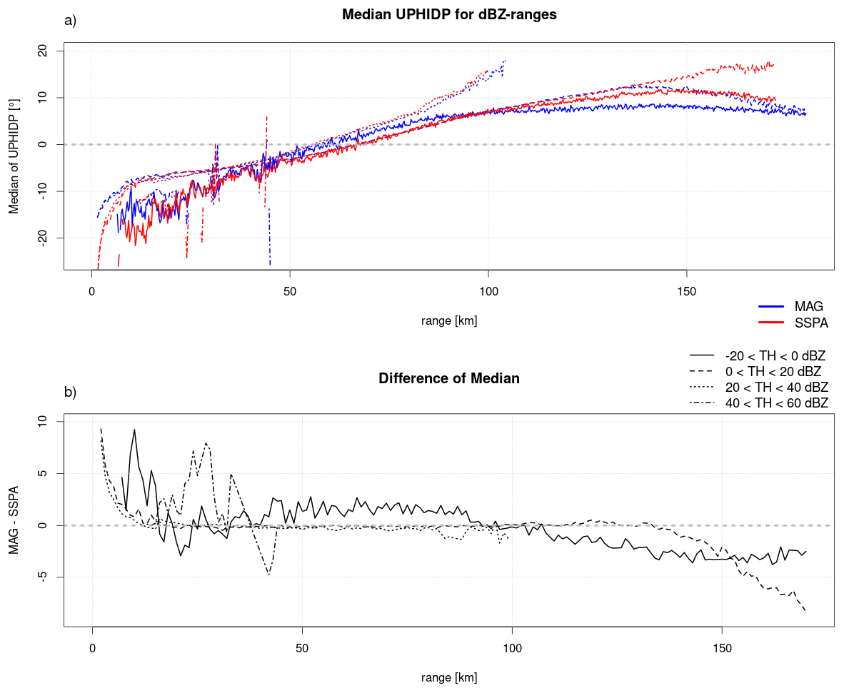
The data collected during the stratiform event is shown in Fig. 14. For both transmitters, the median of the initial PhiDP data was subtracted to achieve an alignment around the 0° line. In contrast to the other radar moments discussed, the lines of all four reflectivity categories match quite well. All show the expected increase in PhiDP-values which is caused by attenuation. The strongest precipitation during the stratiform event fell into the category from 20 to 40 dBZ. The slopes of these lines are therefore the steepest; the difference between MAG and SSPA is close to 0° up to 110 km range. Most other precipitation was recorded with a reflectivity between 0 and 20 dBZ (cf. Fig. 7). The two lines representing this category also match up well to a range of 130 km. Further out, MAG PhiDP drops slowly and finally reaches the noise value (solid line, −20 to 0 dBZ). PhiDP in SSPA continues to rise out to almost the maximum recorded range. With the convective case (not shown), the general findings can be confirmed, but the image is less clear due to the spatially distributed nature of the event.

One parameter used in DWD's quality assurance to identify clutter is the texture of PhiDP. It is defined as the standard deviation of PhiDP in a moving 5 by 5 pixel window. In the centralized DWD radar data quality control, a texture threshold of 15° is used to identify clutter.

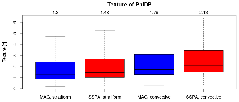
Figure 15 Texture (standard deviation) of PhiDP during both stratiform and convective events. Data is heavily thresholded: Reflectivity is between 20 and 40 dBZ and RhoHV > 0.9. Outliers of the distribution are not shown. Numbers above the boxes are the median values of the respective distributions (including outliers).

For this purpose, we compute the texture from data that satisfy 20 dBZ < TH < 40 dBZ and RhoHV > 0.9. The results for both the convective and the stratiform case are shown in Fig. 15, with the outliers removed. Median values and distributions match very well. The texture of PhiDP from SSPA data can therefore be used in the quality assurance just in the same way as it is done for the MAG data. We were not able to fully confirm why the texture has a slightly higher values in SSPA for both weather cases. Presumably, some measurements fulfill the narrow thresholds used for computing the texture, which are not from precipitation. Clutter or range sidelobes might be responsible, as well as the larger amount of raw range bins being used for one processed range gate in MAG data, which works as a smoothing mechanism.

Figure 16 Like Fig. 10, but for the uncorrected differential reflectivity UZDR.

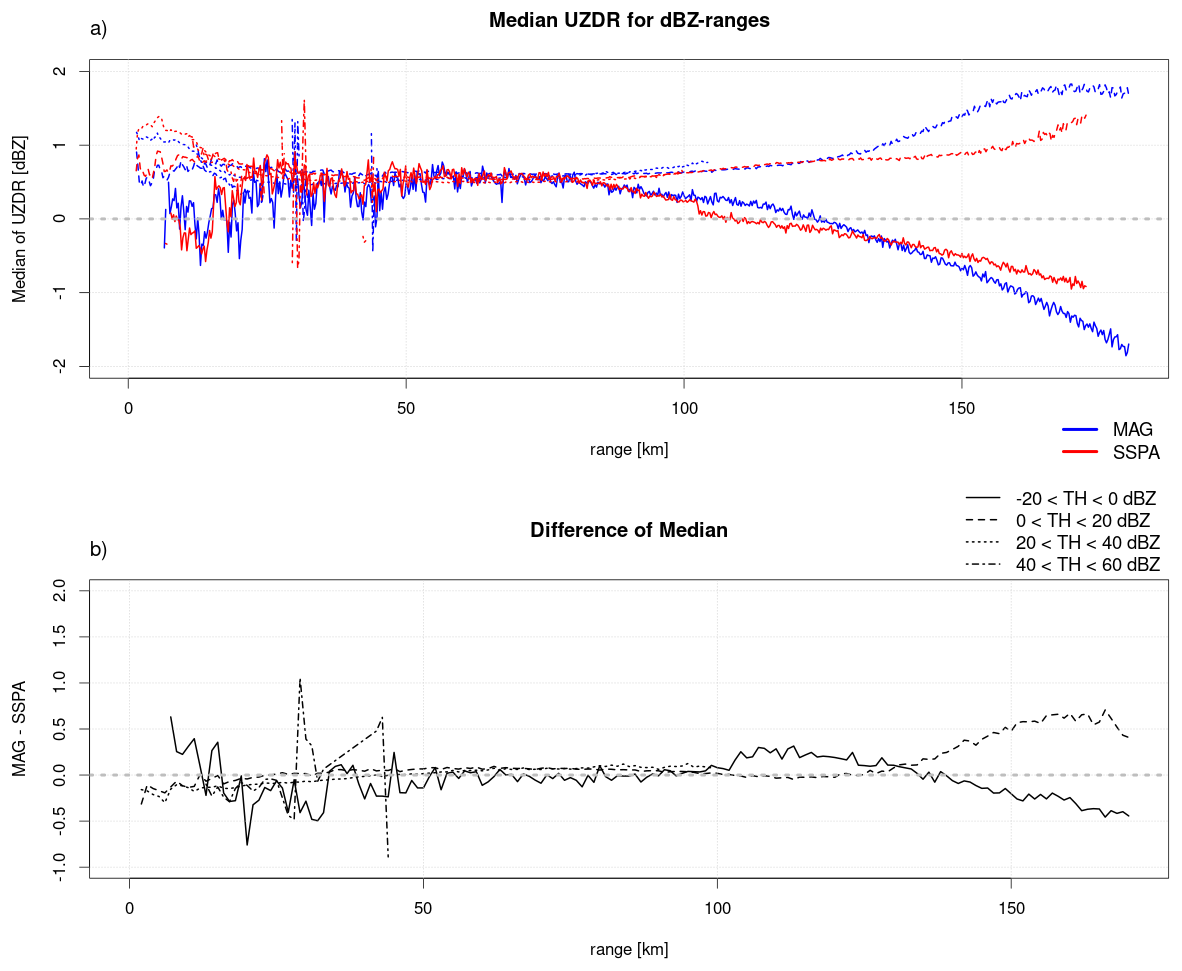
The differential reflectivity ZDR is the quotient of the received power of the horizontal and vertical channels in linear units, or the difference of the two measurements in logarithmic units. It is extensively used in the classification of hydrometeor types (Zrnić et al., 2001). For this purpose, it is required to be determined with a precision of down to 0.1 dB. Figure 16 shows the median ZDR for the stratiform case. It is very clear that the average ZDR within the measured precipitation lies at about 0.6 dB for all reflectivity categories and both transmitter types. This value is too high for the observed stratiform, dry snow (Ryzhkov and Zrnic, 2019), so we attribute this to a miscalibration of the ZDR. Nevertheless, the offsets seem to be identical between the two transmitters, so the data remains comparable.

As described above for the other moments, most precipitation during the 2024 stratiform event falls into the two middle reflectivity categories between 0 and 40 dBZ (cf. Fig. 7). The lines representing the two classes show the best agreement. Near the radar at low range, clutter effects are apparent. Between about 25 and 130 km, MAG and SSPA measured an almost identical ZDR. Differences are below the targeted 0.1 dB, as can be seen in Fig. 16b. Beyond 100 km range, reflectivity values are between 0 and 20 dBZ. MAG and SSPA agree well up to a range of 130 km. At larger ranges only SSPA data show a credible value, while the UZDR in MAG drifts towards a unnaturally high value. In the lowest category for TH between −20 and 0 dBZ, MAG and SSPA agree reasonably well, as long as there are valid measurements. After about 80 km, UZDR for both transmitters starts dropping, indicating the absence of valid measurements and the transition into noise. The data for the convective case shows very similar characteristics, but it is less clear due to the distributed nature of the precipitation.

3.5 Matching the un-modulated short pulse with the modulated long pulse

The presented SSPA transmitter uses a two-pulse scheme. A short, un-modulated pulse is used to fill the blind zone that cannot be covered by the modulated long pulse. The matching of short and long pulse in phase and power is a step done after the absolute calibration of the short pulse. Raw power samples are taken during stratiform rain where the short and long pulse overlap. Long pulse power measurements are then iteratively corrected with an offset, until no discontinuity in the data between long and short pulse is visible. This offset is found to be constant over a long time under the assumption that neither pulse modulation nor radar hardware changes.

In a first step, the short pulse is calibrated using a known signal, e.g. from a signal generator. Then the radar is set into an operational state during precipitation. Offsets for both horizontal and vertical power and also phase are then chosen such that the transition between short and long pulse at a range of 16 km appears smooth in an A-scope or comparable depictions. The offsets are applied to the digitised I&Q time series in the signal processor, so that the finished radar moments do not have any visible gap or overlap areas. Furthermore, the IFD continuously records data from the transition range and resulting offset estimates are written into the radar status information. A dynamic adjustment of offsets is possible and implemented in the signal processor. However, this option has not been used so far, as the initially chosen offsets have been proven to be stable. Values from continuous offset monitoring since the installation of the system have only deviated slightly from the initial offsets.

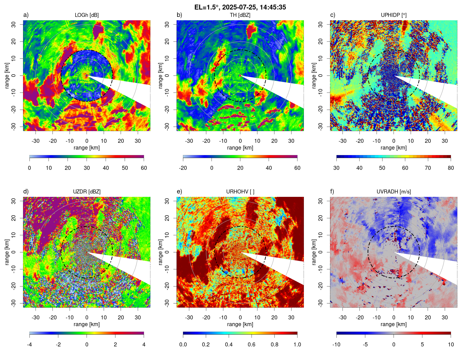
Figure 17 PPIs of (a–f) logarithmic power LOG, reflectivity TH, differential phase PhiDP, differential reflectivity UZDR, correlation coefficient RhoHV and Doppler velocity UVRADH. Data taken with the SSPA transmitter during the convective event in July 2025. Shown are the inner 30 km of range. The black dashed circle marks the border between short and long pulse.

Figure 17 shows PPIs of several radar moments during the already presented convective case. The image is zoomed to the inner 30 km of range and the black dashed circle marks the range where short and long pulse meet (15.2 km). Figure 17a shows the raw received power in logarithmic scale, called “LOG”. The precipitation areas are clearly visible in both the short and long pulse ranges, but the absolute values in the short pulse range are substantially lower due to the lower transmitted energy. This moment is used for internal calculations and not for any meteorological applications, but it clearly shows the characteristics of the pulse gap.

The other five moments in Fig. 17 (Reflectivity, differential phase, differential reflectivity, correlation coefficient and radial velocity) show no pulse gap during the selected time step, proving that the pulse matching with fixed offsets works as intended. Additionally, the line plots in the previous sections (Figs. 6, 10, 13, 14 and 16) can be used to further investigate the gap. It can only be seen in RhoHV within areas low reflectivity. The other moments show no gap. The offsets are tuned towards matching the measurements taken in precipitation.

Most issues caused by the two-pulse scheme and the necessary matching may be solved by using the long pulse return for the short-pulse range as well (Salazar Aquino et al., 2021; Malkomes, 2025). This will be tested with our radar setup in the future.

3.6 Range sidelobes

If a strong target is detected with a modulated pulse, like a strong clutter target or a convective core, some of the measured signal power will be visible in adjacent range gates in front of and behind the strong target after pulse compression. If the actual target is sufficiently strong, the corresponding range-time sidelobe may raise the power to a level that is comparable with radar moments in typical weather. The shape of the pulse with the implemented frequency modulation and some additional tapering can be used to suppress range sidelobes up to a certain strength, but this comes at the expense of range resolution. Range sidelobes in the data take effect over the entire length of the transmitted pulse, i.e. 30 km for a 100 µs pulse.

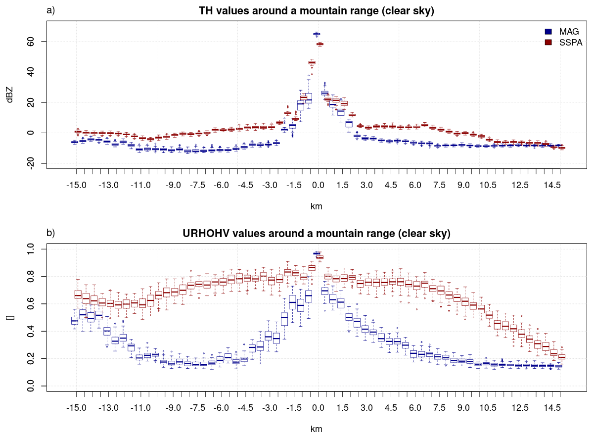
Figure 18 (a) Uncorrected reflectivity (TH) and (b) correlation coefficient (URHOHV) around a mountain range during a clear sky case. Data collected over 60 sweeps per transmitter and linearly interpolated to a common range.

The SSPA range sidelobes of the presented radar are investigated by looking at strong clutter returns from the Alps in the south of the radar. The typical effect is shown in Fig. 18 for a clear sky case, and their appearance in a PPI can be seen in Figs. 4 and 17. Data from around a known mountain chain at 30 to 60 km range and 163 to 172° AZ are cut out from 60 sweeps per transmitter taken at 1.5° elevation. The data from each sweep are centered on the maximum value of TH per ray, averaged over the selected azimuth angles and then interpolated to a common range grid with a 500 m resolution. Results for TH are shown in the top panel. First, the TH peak reaches a maximum at about 60 dBZ. It is lowered by the range interpolation, the actual values reach up to 70 dBZ. The MAG measurements drop steeply in front of and behind the mountains. At a distance of only 3 km from the peak, the magnetron data already show values between −5 to −10 dBZ, a clear sign that only noise is left in the data. In contrast, higher TH levels between 0 and 10 dBZ are found for the SSPA up to a range of ±10 km, and the value of the MAG is reached only at a distance of approximately 11 km behind the clutter target. The area in front of the strong clutter is influenced by clutter as well, so the measurements do not match up exactly. The pulse form used at DWD's SSPA radar has a suppression capability of −60 dB for the peak sidelobe level (PSL) and −55 dB for the integrated sidelobe level (ISL). The observed level of the range sidelobes matches the PSL: in the range averaged data, the peak power is at 60 dBZ and the sidelobes at 0 dBZ, while the clutter reaches 70 dBZ in the unmodified data and the sidelobes appear with about 10 dBZ in Fig. 17.

The bottom panel of Fig. 18 shows the corresponding RhoHV values. It is very clear that range sidelobes not only raise the reflectivity, but also have a distinct influence on dual-polarization moments. RhoHV values in the averaged MAG data are between 0.6 and 0.8 for ranges close to the strong target and quickly drop off down to 0.2 further out. For the SSPA, RhoHV reaches a comparable peak value but stays over 0.6 up to a distance of about ±10 km. This static clutter example shows that corresponding range sidelobes might reach reflectivity or RhoHV values that are usually interpreted as weather echoes. This complicates the filtering, since the dual-polarization information that might otherwise be used to separate meteorological and non-meteorological signals is contaminated as well.

The same analysis for the static clutter area shown in Fig. 18 was done for a case with precipitation (the 2024 stratiform event, not shown). Here, the range sidelobes are masked by the actual weather and both MAG and SSPA show similar results. RhoHV is close to 1 (as expected for this type of precipitation) and the mountains as such cannot be distinguished from the surroundings using this radar moment. However, the mountains still show a strong in radar reflectivity signal (TH of ≈ 72 dBZ), identical to the clear sky case (Fig. 18). In the vicinity, both MAG and SSPA measure a radar reflectivity of 20 dBZ in precipitation, with almost identical statistical properties (quantiles are the same). Range sidelobes caused by clutter do not affect the measurements significantly, as the meteorological signal is larger than the range sidelobe signal by a factor of about 100. This is true when the clutter target is covered by precipitation homogeneously and over the whole length of the pulse. With smaller precipitation areas, where only parts of the complete pulse length contain precipitation, the separation of weather and range sidelobes becomes increasingly difficult.

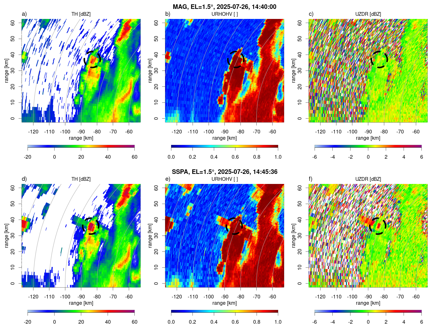
Figure 19 Example of range sidelobes around a convective core, recorded on 26 July 2025. Shown are TH, URHOHV and UZDR for MAG in panels (a)–(c) and for SSPA in panels (d)–(f). The black dashed circle shows the precise location of the convective core. Small differences between the two transmitters are caused by the five minute time difference in which the strength of the convective core increased.

Range sidelobes do not only appear around clutter, but are also caused by strong meteorological targets, with shape gradients in range. Figure 19 shows range sidelobes in the presence of a convective cell for TH, URHOHV, and UZDR in comparison to the results from MAG. Data was recorded during 26 July 2025. Clearly, range sidelobes blur the actual cell in the radial direction for all three moments shown here. The cell core has a reflectivity on the order of 60 dBZ. With an ISL of −55 dB a 5 dBZ signal may be expected. This magnitude can be seen in the actual data where we see a line shaped structure with a length of about 15 km in the radial direction from the convective core (circled feature in Fig. 19). The consequence of this on the performance and skill of e.g. DWD's convective cell tracking algorithm KONRAD3D (a basic description can be found in Werner et al., 2024) will be investigated in a follow-up study. Similar shapes caused by the lightning protection system of the radars (Hald et al., 2024) have not shown negative effects on products like KONRAD3D.

To conclude, range sidelobes are inherent when pulse compression is applied to localize radar echoes based on a long, frequency modulated pulse. Even though the implemented signal processing is able to achieve an ISL of -55 dB, in the presence of strong targets (ie. clutter, thunderstorms with hail cores) range sidelobes appear in all of the radar moments, especially in the dual-polarization moments. The length scale of range sidelobes is inherently limited to the length of the long pulse which is in our case about 30 km.

3.7 Clutter suppression

The term clutter, in the context of weather radars, describes the measured signal power in radar data that is reflected from non-meteorological scatterers. In most applications, the word is simply used for ground clutter. Due to the fact that most of these scatterers have a Doppler velocity close to zero, weather radars are able to remove their influence from the measurements using signal processing methods. One prominent method is the use of DFT or FFT filters. The received I&Q time series is transformed into its spectrum. Spectral parts that are within a definable interval around the 0 m s⁻¹ radial velocity are removed and interpolated, before the data is re-transformed into a time series again (Siggia and Passarelli, 2004). Other clutter filters, like for example recently proposed regression filters (Hubbert et al., 2021), work with the same assumption of clutter being the non-moving part of the back scattered signal.

This section examines if both MAG and SSPA transmitters achieve a comparable level of clutter suppression. As described in Sect. 2.2, both use the same Doppler clutter filter with identical settings. The filter outputs the clutter correction CCORH and CCORV as standard radar moments for the horizontal and vertical polarization channels. These quantities represent the change in signal power caused by clutter filtering, usually expressed in dB. Since clutter filtering removes power from the uncorrected signal, the correction is defined as a negative value.

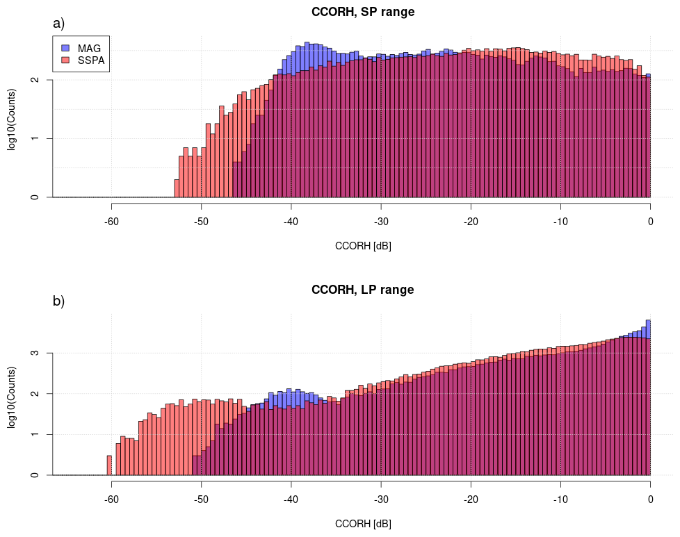
Figure 20 Distribution of CCORH values in two sweeps of SSPA in red and MAG in blue. Data recorded during clear sky conditions on 20 April 2025. (a) Short pulse range or inner 16 km, (b) long pulse range. Counts are displayed in a logarithmic scale.

The distribution of CCORH values from two consecutive sweeps from MAG and SSPA during a clear sky case is shown in Fig. 20. The top row shows the frequency of occurrence of CCORH values for the short pulse region. Minimum observed clutter power from the SSPA is −53 and −47 dB from MAG. The larger SSPA CCOR is in parts attributed to the improved pulse-to-pulse coherence of the SSPA compared to the MAG, resulting in less leakage of clutter power to adjacent velocities, and to combination of pulse compression and the associated signal processing. Those minimum values are attributed to known clutter targets such as a TV tower in about 1.2 km distance from the radar, which are within the main beam of the antenna. The frequency of CCOR values around −38 dB is about a factor of two larger for MAG compared to SSPA (note the logarithmic scale). This is attributed to the significantly higher transmit power of the magnetron transmitter compared to the SSPA (500 kW vs. 10.3 kW). Though the short pulse results in reduced sensitivity in a range of up to 16 km, at the same time less ground clutter power is picked up through the antenna sidelobes. As a side note, a CCORH threshold of −15 dB is currently applied to the radar reflectivity in the DWD radar network.

The bottom row shows CCORH for the long pulse range. At values below −35 dB, both transmitters show a distinct maximum: MAG at around −40 dB, and SSPA at around −50 dB. The Alps south of the radar cause these distinct CCOR values. The specific SSPA system with its higher coherence compared to a MAG transmitter leads to an improved clutter separation in the received time series.

We were able to confirm these findings with data of the vertical polarization channel.

4 Discussion and Conclusions

This paper described a weather radar with a unique dual transmitter setup at DWD's observatory Hohenpeissenberg. Magnetron and solid state power amplifiers share the same hardware like waveguide, antenna and pedestal. The active transmitter can be switched via software within a few seconds. This creates a valuable test setup for the evaluation of SSPA weather radar data against known magnetron quality. Differences in the data can be fully attributed to the differences of the transmitters and a short time offset. The main purpose of the setup is to investigate whether SSPA data can reach the same data quality compared to MAG data and to identify and quantify possible differences. Future setups could use the fact that SSPA transmitters can be build substantially smaller than MAG transmitters and can therefore be placed over elevation at the back of the antenna. This minimizes waveguide losses and avoids the necessity of a waveguide rotary joint, among other advantages. Weather radars with such a design are already available on the market.

To investigate the data quality, sweeps from both transmitters recorded at an elevation of 1.5° during one stratiform and one convective event were used. In terms of reflectivity we find that both transmitters show a very good agreement. A side-by-side comparison shows comparable magnitude and location of precipitation echoes from stratiform and convective precipitation events. Additionally, we find that SSPA, due to the pulse compression in the modulated long pulse, has a higher sensitivity. This translates to a better detection of weak precipitation and to a better performance at ranges larger than 130 km. In the short pulse range on the other hand, SSPA lacks sensitivity. At 16 km range, a minimum reflectivity of about −5 dBZ can be measured compared to about −15 dBZ for the magnetron system.

In terms of Doppler velocities, we also find a good agreement between the transmitter types. No gap between short and long pulse is visible. At ranges larger 130 km, the higher sensitivity and coherence of the SSPA produces more meaningful measurements than MAG. While precipitation has to be on the order of 20 dBZ in MAG for valid Doppler data, the SSPA can gather information down to a reflectivity of 10 dBZ or less. These findings are limited to the described 1.5° elevation scans with a staggered PRF of 600 to 800 Hz and a $\mathrm{3}/\mathrm{4}$ unfolding ratio. It is known that the uncertainty of the measurements increase when higher unfolding ratios are used (Hengstebeck et al., 2018), but these might be necessary with SSPA due to some hardware limitations: DWD's MAG has a duty cycle of $\mathrm{1}/\mathrm{1000}$, so it can use a short pulse of 0.4 µs with a maximum PRF of 2500 Hz. This is sufficient for DWD's requirement to resolve Doppler velocities to ±32 m s⁻¹ without staggering. The SSPA has a much higher duty cycle of about $\mathrm{1}/\mathrm{10}$. However with a total pulse length of 100 µs, the maximum PRF for this system is 1000 Hz, translating to a Nyquist velocity of about 13 m s⁻¹ in C-Band. Staggered PRF and unfolding are therefore needed to achieve the DWD requirement for the unambiguous velocity range. The implications of that on other parameters, like maximum unambiguous range, antenna rotation speed and the pulse sample size per ray have to be kept in mind when conceptualizing a scanning strategy for an SSPA radar. Future experiments could use a shorter duration for the long pulse, especially at high elevations where range is less of an issue, to be able to increase the PRF.

The dual-polarization moments differential phase PhiDP, correlation coefficient RhoHV and differential reflectivity ZDR were evaluated in the same way as the other moments. PhiDP and ZDR showed good agreement with the MAG measurements. Results match over the full range of reflectivity and effects at the border between short and long pulse are negligible. SSPA values at ranges over 130 km are more reliable than in MAG due to the higher coherency of the SSPA system. RhoHV in the long pulse range of the SSPA is much more reliable than MAG. High values can be measured in much weaker precipitation or at larger ranges. SSPA has disadvantages in the short pulse range: the un-modulated short pulse behaves like the MAG pulse, but with the addition of much lower power and therefore less sensitivity. Data at the maximum short pulse range therefore shows the same properties as with MAG: RhoHV in weak precipitation degrades when SNR falls under a certain threshold.

Using a long, modulated pulse with the SSPA results in a blind zone close to the radar. The presented setup uses an additional, un-modulated short pulse to fill this zone. The two pulses are independent, and the data at the border has to be matched. In the presented case, fixed offsets for signal power and phase are used. This simple approach works well and the gap can barely be seen in the data, as long as it contains weather. Still, the degradation of the data at the maximum range of the short pulse is visible, especially in the correlation coefficient RhoHV. The low transmitted energy in the short pulse is not able to properly resolve weak precipitation. Recent developments in using the long pulse return for the range close to the radar might make the short pulse obsolete, and the issue might be fully mitigated.

The main issue observed in the SSPA data are range sidelobes. They are an effect of the pulse compression. Measured properties of a strong target, like clutter or convective cores, leak into all adjacent range gates, spanning the whole length of the pulse. Despite a high sidelobe suppression of 60 dB, we were able to observe the enhanced signal around strong targets. In clear sky, this leads to an increased level in reflectivity of about 10 dBZ compared to the MAG. One major issue of range sidelobes is that they also contain the properties of the target with large reflectivity. Therefore, range sidelobes may have a high RhoHV and a homogeneous differential phase, meaning that these moments can not be used to identify and remove range sidelobes.

Clutter suppression of the two systems was investigated with clear-sky data. In general, the SSPA has a higher suppression in both the short and the long pulse due to the higher coherency of the system. In the short pulse range, the SSPA additionally profits from the lower transmit power, which lets the system avoid a lot of clutter though the antenna side lobes, as it can be seen in the MAG data. In the long pulse, clutter suppression is, on average, 10 dB better than MAG, with a maximum of −60 dB.

In the same way, range sidelobes caused by clutter will be recognized by the clutter filter, which will return an enhanced clutter power. This can help to remove the sidelobes caused by stationary clutter, but will not help for those caused by precipitation. We believe that more effort is necessary in trying to find pulse shapes that further minimize range sidelobes. Additionally, filtering techniques (during runtime or ex post) might be developed.

The presented data was recorded with signal processing settings that tried to match those of the magnetron radar as close as possible. One next step in the evaluation of the system will be to see whether different settings, e.g. different clutter filtering techniques and adapted thresholds, can further increase the data quality of the SSPA. Then, the data will be supplied to the processing chain that is used for radar data at DWD. Within this chain, a multitude of different products for different use cases is generated, for example cell tracking, mesocylone detection, hydrometeor classification and quantitative precipitation estimation. The goal is to find out if the data from a SSPA radar can be used “out of the box” for those products or if major adaptions are necessary.

In summary, with this unique setup where we have incorporated a SSPA transmitter into a DWD magnetron weather radar, we can show that the SSPA transmitter is able to produce data that have comparable quality compared to a magnetron transmitter. In some cases we find superior quality, in particular at low SNR in the long pulse region. Based on our findings regarding data quality, SSPA is a suitable replacement for magnetron transmitters in the next generation DWD weather radar. Signal processing techniques for SSPA are still in ongoing development, so the range sidelobes, which were identified as an issue, might be circumvented in the future.