Modelling monthly Boundary Layer Height maps combining radiosonde, satellite, and reanalysis over Europe

The height of the planetary boundary layer directly influences local and regional climatic phenomena, making its study and estimation of vital importance for environmental sciences. The main objective of this work was to create a gridded map of planetary boundary layer height across the European continent, with a spatial resolution of 25 km and monthly mean values at two synoptic hours (12:00 and 00:00 UTC). We implemented the regression kriging method by combining various data sources, including observations, climatic and topographic variables, and reanalysis data (ERA5), and different regression methods (linear, random forest, and gradient boosting) for the 2010–2020 period. In both UTC hours, combining reanalysis, land surface temperature and topographic covariates with random forest regression provided the best performance. However, the models' performance at night declined considerably compared with midday. Then, we compared our seasonal predictions with reanalysis data and found a consistently higher spatio-temporal accuracy than that of the ERA5 reanalysis. For example, at 12:00 UTC, spatial variability in winter showed RMSE values ≤170 m, compared with ≥250 m for ERA5, while temporal variability in summer reached RMSE values ≤260 m, versus 340 m for ERA5. At 00:00 UTC, spatial variability in summer achieved RMSE values = 14 m, whereas ERA5 exhibited RMSE = 60 m, while temporal variability in winter reached RMSE values ≤176 m, versus 200 m for ERA5. The proposed regression kriging method thus performed well in estimating the height of the boundary layer at 12:00 UTC, and to a lesser extent at 00:00 UTC.

1 Introduction

The Boundary Layer (BL) is the lowest part of the troposphere in contact with the Earth's surface, responding on short time scales to surface atmosphere exchanges of heat fluxes, solar radiation, pollutant emissions, moisture, momentum, land cover, and topography. The dynamics of the BL are strongly influenced by the diurnal cycle. Consequently, two contrasting situations can be observed in terms of BL characteristics. During the day, a deeper and more turbulent convective boundary layer develops, driven by convective thermals generated by sensible and latent heat fluxes. In contrast, after sunset, radiative cooling of the ground or the advection of warm air over a colder surface leads to the formation of a shallow and less turbulent stable boundary layer at night (Stull, 1988).

The height of the boundary layer (BLH), that is, how deep it can become during the day and how shallow it remains at night, represents a key parameter in meteorology and is typically defined as the altitude of the inversion layer that separates the free atmosphere from the planetary boundary layer (Stull, 1988). Its top defines many tropospheric processes that influence climate and air quality, such as the transport, transformation, and mixing of aerosols and pollutants (Seibert et al., 2000; Zhang et al., 2013). Therefore, the role of BLH in climatological processes and in sustaining a healthy environment for human life makes its study a highly relevant topic in environmental sciences.

In practice, estimating the BLH at different times of the day is a real challenge, as it results from a multitude of processes acting simultaneously across a wide range of spatial and temporal scales. The factors influencing its estimation may vary across different regions of the Earth. For instance, solar radiation strongly drives latitudinal differences, with greater BLH values at mid- and low latitudes compared to higher latitudes (Guo et al., 2021).

Seasonality also plays a key role: in some regions, BLH tends to be higher in spring and summer, and generally lower in autumn and winter (Guo et al., 2019; Saha et al., 2022). In other regions, however, it reaches its greatest depth in summer and its shallowest extent in winter, with transitional values observed in spring and autumn (Nelson et al., 2021; Li et al., 2023). Seasonal rainfall patterns and dry periods exert a strong influence on BLH as well, directly modulating its variability (Dias-Júnior et al., 2022; Li et al., 2023). At higher altitudes, however, this seasonal pattern may be reversed, since topography is another critical driver of BLH (De Wekker and Kossmann 2015).

Regardless of the inherent complexity and variability described above, BLH estimation also varies depending on the mathematical approaches applied and the diversity of instruments used to obtain the input data. These factors introduce biases among the different procedures implemented to determine BLH (Seibert et al., 2000; Chen et al., 2023; Roldán-Henao et al., 2024; Zhang et al., 2025). Most methods for calculating the top of the BL rely on vertical profiles of climatic variables, including temperature, pressure, wind, humidity, water vapor, and refractive index (Seibert et al., 2000; Seidel et al., 2010). In practice, these profiles can be obtained from radiosondes or ground-based remote sensing instruments (e.g., LIDAR, SODAR, microwave radiometers, among others). Alternatively, BLH estimates can be obtained from reanalysis products (Seibert et al., 2000; Guo et al., 2021; Saha et al., 2022).

Reanalysis products are a powerful tool with notable advantages over other approaches. They combine real-world observations with numerical model forecasts and data assimilation. This integration provides consistent estimates of atmospheric, surface, and oceanic parameters for all locations worldwide, with no spatial gaps (Teixeira et al., 2021). Numerous studies have evaluated the efficiency with which reanalysis can reproduce the daily dynamics of the boundary layer. Evidence indicates that the BLH from ERA5 (the fifth-generation ECMWF reanalysis) is reliable when compared with observational datasets, showing correlations close to r=0.9 and biases ranging from a few metres to more than one kilometre. Nonetheless, findings also reveal systematic underestimations or overestimations of BLH from ERA5 at specific times of day and the study region (Guo et al., 2021; Sinclair et al., 2022; Dias-Júnior et al., 2022; Slättberg et al., 2022; Li et al., 2023).

Recent advances in modelling approaches that integrate observations, remote sensing data, and reanalysis to predict BLH values have yielded promising results (Ayazpour et al., 2023; Guo et al., 2024; Zhang et al., 2025). This progress highlights the inherent complexity of the numerous processes operating simultaneously across a wide range of spatial and temporal scales. In this context, the continuous spatio-temporal coverage provided by reanalysis is particularly valuable (Sinclair et al., 2022; Guo et al., 2024). Its application to the generation of gridded maps, in combination with other variables, enables the production of more refined BLH representations (Ayazpour et al., 2023). By offering a more accurate baseline for analysing BLH trends and variability, including their climatic impacts, these products may serve as a reference for evaluating regional climate models and for the development of high-resolution regional climate change scenarios.

To this end, the present study aims to generate observation-constrained gridded boundary layer height (BLH) maps for Europe using a hybrid regression-kriging framework. More specifically, the study will (1) Model a gridded map of BLH using observational data from radiosondes (BLH_RS), combined with BLH derived from reanalysis (BLH_ERA5) and climatic and topographic variables. (2) Evaluate the accuracy of the resulting observational gridded maps against observational data, both spatially and temporally.

The remainder of this paper is structured as follows. Section 2 describes the datasets, covariates and methods employed to create and evaluate the models. Section 3 presents the performance of the models. Section 4 provides a discussion of main results and finalizing with concluding remarks in Sect. 5.

2 Data and Methodology

2.1 Study area and BLH from radiosonde

This study covers the European continent, encompassing diverse climatic and topographic regimes. The planetary boundary layer height radiosonde data (henceforth BLH_RS) employed here were derived from observations originally compiled in a previous work. Briefly, radiosonde data were collected between 2010 and 2020 from several weather station sources. For each launch, vertical profiles of wind, pressure, temperature, relative humidity, and dew-point temperature were extracted. These data were then processed to estimate BLH_RS using the bulk Richardson number method (see Salcedo-Bosh et al., 2025 for methodological details). Accordingly, our focus here is on the procedures applied to manage and process these data.

The dataset comprises 129 stations (Fig. 1a), which were filtered according to two specific times representing contrasting stages of the planetary boundary layer: at 12:00 UTC, which is related to the convective boundary layer phase, and at 00:00 UTC related to the stable boundary layer. Therefore, it is assumed that each day provides one measurement for each of these times. To ensure data quality, only launch stations with at least 45 % daily coverage, equivalent to more than 1800 d of data per station, were retained for the analysis. Due to the sparse temporal coverage of the dataset, monthly mean BLH values were used for both assessment and interpolation.

Each meteorological station was verified and georeferenced using the University of Wyoming Atmospheric Science Radiosonde Archive (https://weather.uwyo.edu/upperair/sounding.shtml, last access: 20 September 2025) to obtain the station name and the exact launch coordinates (latitude and longitude in EPSG:4326). Figure 1b and c illustrate the spatial distribution of the selected stations for each observation time, including 44 stations at 12:00 UTC and 39 stations at 00:00 UTC. The minimum distance between stations was 170 km for the 12:00 UTC dataset, with an average distance of 1871 ± 1021 km. For the 00:00 UTC dataset, the minimum distance was 180 km, with an average distance of 1875 ± 1043 km.

Figure 1 Map of the launch stations considered in the study. (a) Pool of stations available for the Europe region (12:00 and 00:00 UTC). (b) 12:00 UTC stations with at least 45 % of daily data for the 11 years (N=44). (c) 00:00 UTC stations with at least 45 % of daily data for the 11 years (N=39).

2.2 Covariates

As our objective was to obtain an improved gridded map, the selected covariates were those related to boundary-layer development, either directly or indirectly influencing the height of the capping inversion, and available in gridded format. Furthermore, within the extensive range of available data sources, we prioritized covariates derived from independent origins (instrumental, methodological, or both) to minimize potential error propagation associated with the limitations of a single data source (Hengl, 2009). Furthermore, preference was given to datasets with the highest possible spatial resolution, ensuring a more accurate representation of the local conditions at each station. Below, we briefly describe the relevance and sources of the data considered in this study.

2.2.1 Reanalysis data

Of the available reanalysis products, we used ERA5 because, in comparison with other reanalysis products such as MERRA-2, NARR, NCEP-2 and JRA-55, it has shown good correlation with BLH values derived from radiosondes (Guo et al., 2021; Ayazpour et al., 2023). Although far from perfect, the accuracy of reanalysis products is often affected by seasonality (with larger errors during the warm months), topography, and other factors. Such discrepancies are frequently attributed to model parametrisations that do not accurately reflect real-world conditions (Guo et al., 2021; Dias-Júnior et al., 2022).

In ERA5, the boundary layer height (henceforth BLH_ERA5) is provided on a 1440×721 grid with a spatial resolution of 0.25° in both latitude and longitude. It is calculated using the bulk Richardson number method, with a temporal resolution of one hour. We downloaded boundary layer height data from Copernicus Climate Service (https://cds.climate.copernicus.eu/datasets, last access: 7 July 2025) at 12:00 and 00:00 UTC for the full study period (2010–2020). BLH_ERA5 values were then extracted for each station by matching date, hour, and latitude and longitude, with the nearest BLH_ERA5 grid point assigned to each location. With these values, we calculate the monthly BLH_ERA5 by station. Then we used the gridded map of monthly averages (11 years) at 12:00 and 00:00 UTC for the interpolation procedures. In the present study, ERA5 represented the coarsest spatial resolution (0.25° × 0.25°) among the evaluated datasets, while providing the finest temporal resolution, with hourly data availability.

2.2.2 Temperature and wind

Temperature plays a central role in the surface energy balance, which depends not only on solar radiation (e.g., the daily cycle) but also on soil moisture and land surface cover (Pal Arya, 1988). Therefore, it is a powerful predictor of the spatio-temporal evolution of BLH (Guo et al., 2021; Madonna et al., 2021). Wind, in turn, is a fundamental component of the boundary layer, responsible for the horizontal and vertical transport of moisture, heat, momentum, and pollutants. Both variables are positively associated with BLH (Guo et al., 2016) and are also explicitly considered in BLH estimation methods (Seibert et al., 2000; Seidel et al., 2010). Hence, their inclusion as covariates is a natural choice.

Land surface temperature from satellite (MODIS)

MODIS (Moderate Resolution Imaging Spectroradiometer) is an instrument onboard NASA's Terra and Aqua satellites with different orbits. One of its products is Land Surface Temperature (LST) available at daily, 8 d, and monthly temporal resolutions, and at spatial resolutions of 1 and 5 km. We compared the LST values from both satellites at each target time, given that the product is reported as “daytime”/“night-time” rather than hourly data. Specifically, we examined how well Aqua (around 01:00–02:00 pm over Europe) versus Terra (∼10:00–11:00 am) “daytime” LST values aligned with BLH_RS at 12:00 UTC, and Aqua (01:00–02:00 am) versus Terra ($\sim \mathrm{10}:\mathrm{00}$–11:00 pm) “night-time” LST values with BLH_RS at 00:00 UTC. This comparison allowed us to select the most suitable dataset for interpolation and further analysis.

We extracted LST values, Aqua (MYD11A1)/Terra (MOD11A1) (daytime and night-time) at 1 km spatial resolution for each radiosonde launch station and date. With these daily values, we calculate the monthly LST${}_{\mathrm{Terra}/\mathrm{Aqua}}$ by station and UTC. For the interpolation procedure, we employed monthly mean LST data, extracted from Aqua (MYD21C3) and Terra (MOD21C3) (daytime and night-time) at 5 km resolution, which were subsequently resampled to 0.25° × 0.25° to match the resolution of ERA5 data. To ensure reliability, LST pixel values were filtered using data quality flags (bits 3 and 2), retaining only those with QA = 0 (good quality), since unreliable or unquantifiable pixels could bias the analysis. Consequently, we had some missing pixel data caused by cloud cover, poor input data, or calibration issues, which often resulted in fewer daily LST records than available in the observational dataset. All these steps were performed in Google Earth Engine.

Air temperature and wind speed from observation assemblage (E-OBS)

E-OBS (v31.0e) is an observation-based gridded dataset, available at daily temporal resolution and spatial resolutions ranging from 0.1 to 0.25°. The E-OBS gridded maps are produced by averaging 20 spatial simulations, each constructed using spatial correlations derived from the underlying observational network. As it is based on observational input, the spatial extent of E-OBS is more limited compared with that of other available products (e.g., LST). Accordingly, the study area when using this dataset is restricted to approximately 25–71.5° N latitude and 25° W–45° E longitude.

A priori, it was unclear which E-OBS product would be most representative. Specifically, whether daily mean or maximum temperature would best reflect BLH at 12:00 UTC, or whether daily mean or minimum temperature would be more appropriate for BLH at 00:00 UTC. To address this uncertainty, we downloaded all three available temperature products-daily mean temperature (TG), daily minimum temperature (TN), and daily maximum temperature (TX) at 0.1° of spatial resolution – for a posteriori comparison – from https://surfobs.climate.copernicus.eu/dataaccess/access_eobs.php (last access: 17 July 2025). Moreover, we downloaded daily mean wind speed (FG) data (Cornes et al., 2018).

We extracted the variable values by station using latitude-longitude and date; however, it should be noted that these values are daily, rather than hourly data (ERA5) or day/night segments (LST). Consequently, for the interpolation procedure, we employed monthly averages (11 years) for TG and FG, using the same gridded monthly maps for both 12:00 and 00:00 UTC interpolation (resampled to 0.25° × 0.25°). The spatial coverage of E-OBS slightly restricts our dataset, which extends further eastward in Europe, close to 50° E. As a result, fewer stations were available for the analyses.

2.2.3 Topography and geographic location

Landscape topography was considered as an additional covariate for BLH. The presence of valleys, basins, and plateaus interacts with mountain waves and thermally driven wind systems, thereby influencing BLH development (De Wekker and Kossmann 2015). Topography also directly affects the altitude starting point of the boundary layer. In this study, the altitude and ruggedness of the terrain were considered as topographic variables.

Furthermore, geographic position may also be related to the intensity of thermal convection (Guo et al., 2021). However, the influence of geographical location (e.g., mid-latitude or tropical) on boundary layer evolution remains relatively unexplored (De Wekker and Kossmann, 2015).

Digital elevation model (DEM)

We extracted, for each station, the altitude values from the digital elevation model with 10 m of resolution available on https://dataspace.copernicus.eu/explore-data/data-collections/copernicus-contributing-missions/collections-description/COP-DEM (last access: 8 August 2025). Then, the DEM was resampled to 0.25° × 0.25° of resolution for interpolation procedures.

Terrain Ruggedness Index (TRI)

The heterogeneity of the terrain was quantified using the Terrain Ruggedness Index (TRI) (described by Riley et al., 1999). This index summarizes local elevation variability by calculating the elevation differences within a 3×3 pixel moving window around each location. The TRI was derived from a 10 m resolution Digital Elevation Model (DEM) using the Terrain Ruggedness Index function from the Geospatial Data Abstraction Library (GDAL), available through QGIS (version 3.32). Then, the TRI gridded map was resampled to match with BLH_ERA5 gridded map.

Geographic location (Coords)

In our dataset, geographic coordinates were considered as covariates as was suggested by Hengl (2009). Latitude and longitude were transformed into plain coordinates (EPSG:3035) to estimate the deterministic component of the regression model and for the interpolation method (kriging).

Unlike the other covariates, coordinates, altitude and terrain index do not exhibit daily variability and therefore correspond to constant values for each station.

2.3 Interpolation Method

To perform the interpolation, we applied Regression Kriging (RK), a hybrid geostatistical method that combines classical spatial autocorrelation with secondary data (covariates) to define a background field for predicting the target variable. When input data are sparse, this approach is particularly useful, as it provides additional support for the prediction (Krähenmann et al., 2018).

Briefly, in a classical kriging the predicted value at an unobserved location is calculated as a weighted average of the observations:

$$\begin{array}{}\text{(1)}& \widehat{z}\left(s_{\mathrm{0}}\right)={\sum }_{i=\mathrm{1}}^n{\mathit{\lambda }}_i\cdot z\left(s_i\right)\end{array}$$

$\widehat{z}\left(s_{\mathrm{0}}\right)$ is a target variable at an unvisited location s₀ given its map coordinates, the sample data z(s₁), z(s₂),... z(s_n), and their coordinates. The weights λ_i are chosen such that the prediction error variance is minimized and thus depend on the spatial autocorrelation structure of the variable.

The regression component of RK models the relationship between the target variable (in our case, BLH_RS) and auxiliary environmental variables (covariates) at the sample locations. In its classical formulation, this relationship is assumed to be linear, and the prediction equation then becomes:

$$\begin{array}{}\text{(2)}& {\widehat{z}}_{\mathrm{RK}}\left(s_{\mathrm{0}}\right)={\sum }_{i=\mathrm{1}}^n{\mathit{\lambda }}_i\cdot z\left(s_i\right)+{\sum }_{k=\mathrm{0}}^{\mathit{\rho }}{\widehat{\mathit{\beta }}}_k\cdot q_k\left(s_{\mathrm{0}}\right)\end{array}$$

where q_k(s₀) are the values of the auxiliary variables at the target location, ${\widehat{\mathit{\beta }}}_k$ are the estimated regression coefficients and ρ is the number of auxiliary variables. Once the deterministic part of the variation (regression) is estimated, the residuals, i.e., the variation not explained by the regression, can be interpolated using kriging and added to the estimated trend (Hengl et al., 2007). The regression coefficients (${\widehat{\mathit{\beta }}}_k$) are obtained using Generalized Least Squares (GLS), which explicitly accounts for the spatial correlation among individual observations, defined as follow:

$$\begin{array}{}\text{(3)}& {\widehat{\mathit{\beta }}}_{\mathrm{GLS}}={\left({\mathbf{q}}^T\cdot {\mathbf{C}}^{-\mathrm{1}}\cdot \mathbf{q}\right)}^{-\mathrm{1}}\cdot {\mathbf{q}}^T\cdot {\mathbf{C}}^{-\mathrm{1}}\cdot \mathit{z}\end{array}$$

Here ${\widehat{\mathit{\beta }}}_{\mathrm{GLS}}$ is the vector of estimated regression coefficients, C is the covariance matrix of the residuals, q is a matrix of predictors at the sampling locations (covariates) and z is the vector of measured values of the target variable. C matrix is obtained by modelling the covariance of the regression residuals (deterministic component) using a mathematical model (variogram).

Alternatively, the deterministic component can be estimated using non-parametric machine learning algorithms. In contrast to linear regression, these algorithms do not estimate a vector of regression coefficients (β). Therefore, it is not possible to apply the conventional GLS procedure directly to account for residual spatial covariance. Instead, the residuals obtained from the machine learning model are used to estimate their spatial covariance structure through a variogram. This covariance structure is then used to derive the kriging weights (λ), which determine the contribution of each observed residual to the prediction at a new location.

Summarizing, the final prediction at an unsampled location s₀ is then given by:

$$\begin{array}{}\text{(4)}& {\widehat{z}}_{\mathrm{RK}-\mathrm{ML}}\left(s_{\mathrm{0}}\right)=f_{\mathrm{ML}}\left({\mathit{X}}_{\left(s\mathrm{0}\right)}\right)+{\sum }_{i=\mathrm{1}}^n{\mathit{\lambda }}_i\cdot r_{\mathrm{ML}}\left(s_i\right)\end{array}$$

Here f_ML represents the machine learning function applied to the vector of covariates vector ${\mathit{X}}_{\left(s_{\mathrm{0}}\right)}$ at location s₀ and ${\sum }_{i=\mathrm{1}}^n{\mathit{\lambda }}_i\cdot r_{\mathrm{ML}}\left(s_i\right)$ represents the spatial correction obtained by kriging the machine learning residuals, with λ_i being the kriging weight assigned to the residual at location s_i.

Finally, the robustness of this geostatistical methodology is contingent upon the satisfaction of certain assumptions. Firstly, the assumption of a normal distribution and homoscedasticity of the residuals must be made. Secondly, the assumption of second-order stationarity, i.e. the requirement that the covariance depends solely on the distance between points (Hengl et al., 2007). When using non-parametric regression algorithms, these assumptions apply exclusively to the residuals.

We implemented this method using the PyKrige library (Python), which provides functions for combining kriging with both linear and non-linear regression models to fit the deterministic component (linking with scikit-learn library). Given that the relationship among covariates and boundary layer may be linear or non-linear, the present study employed both parametric regression models, Linear Regression (LR), and two non-parametric algorithms: Random Forest (RF) and Gradient Boosting (GB). To avoid overfitting issues when employing RF and GB, the RandomizedSearchCV function (scikit-learn library) was utilised. In this regard, a number of hyperparameters were defined, including “n_estimators” (from 50 to 200), “min_samples_leaf” (from 2 to 10), “min_samples_split” (from 2 to 10), among others. Subsequently, RandomizedSearchCV automatically tested (20 iterations) and selected the optimal combination (MAE as loss function) using data splits.

For simplicity, and to minimise collinearity among covariates, we developed additive models including up to three predictor variables. BLH_ERA5 was consistently retained as the core variable, as it has previously been used as a predictor of BLH from observation with good performance and relevance in the model (Ayazpour et al., 2023).

2.4 Validation

To enable assessing of the performances of the different models, a cross-validation procedure was performed during training using the K-fold cross-validation function (scikit-learn library). This approach allows the model to be evaluated using all available datasets by splitting the pool of stations into k consecutive folds. Each fold is then used once as the test set, while the remaining k−1 folds are used for training.

Given that the value of (k) in cross-validation is defined a priori and depends, in part, on the number of available samples (sample size), its effect on model performance was evaluated. For datasets comprising at least 35 stations, k=5 was selected, resulting in five validation sets of approximately seven stations each. This choice was related to reducing (k) to 4 increased the RMSE by around 10 % for the three regression models evaluated, whilst increasing (k) to 6 produced only a marginal improvement, with a reduction in the RMSE of around 1.5 %.

For datasets with fewer stations (N<35), k was set to 4, generating four groups with at least six stations per fold. Although increasing (k) to 5 reduced the RMSE by between 5 % and 7 %, this configuration meant having approximately five stations per fold, reducing the representativeness of the validation subsets and potentially increasing the risk of overfitting. On the other hand, reducing (k) to 3 resulted in an increase in the RMSE of around 7 %. Therefore, (k=4) was selected as a compromise between the stability of the error estimate and the spatial representativeness of the available samples.

As the stations in the input dataset may be ordered according to geographical proximity, the shuffle option was applied to randomise the data before forming the folds. To ensure reproducibility, a fixed random seed was used.

Diagnostic parameters

The agreement between radiosonde observations (BLH_RS), and the different models was evaluated using a set of commonly employed statistical estimators calculated during training: The root-mean-square error (RMSE) and the mean absolute error (MAE), to represent the magnitude of error among observed and predicted.

$$\begin{array}{}\text{(5)}& \mathrm{RMSE}=\sqrt{{\displaystyle \frac{\mathrm{1}}{N}}\sum _{i=\mathrm{1}}^n{\left(y_i-\widehat{y_i}\right)}^{\mathrm{2}}}\end{array}$$

$$\begin{array}{}\text{(6)}& \mathrm{MAE}=\sqrt{{\displaystyle \frac{\mathrm{1}}{N}}\sum _{i=\mathrm{1}}^n\left|y_i\right.-\left.\widehat{y_i}\right|}\end{array}$$

where y_i is the BLH_RS, and ${\widehat{y}}_i$ is the predicted values by the model. The value of RMSE and MAE have value 0 if the regression model fits the data perfectly, and positive (without upper bound) value if the fit is less than perfect. MAE in the same units as the target variable, making it intuitive and easy to interpret, while RMSE is sensitive to the presence of outliers (Mundu et al., 2026).

Also, two other parameters for evaluating the model's fit (variance): The coefficient of determination (R²) and the normalized root square error (RMSEr):

$$\begin{array}{}\text{(7)}& R^{\mathrm{2}}=\mathrm{1}-{\displaystyle \frac{{\sum }_{i=\mathrm{1}}^n{\left(y_i-\widehat{y_i}\right)}^{\mathrm{2}}}{{\sum }_{i=\mathrm{1}}^n{\left(y_i-\overline{y_i}\right)}^{\mathrm{2}}}}\end{array}$$

where n is the number of observations, y_i is the BLH_RS, and ${\widehat{y}}_i$ is the predicted value and ${\overline{y}}_i$ is the mean of the observed values. The R² is bounded above by a value of 1, which is achieved when the model provides a perfect fit to the observed data. However, unlike the upper limit, has no lower bound. A value of 0 corresponds to the case where the model performs equivalently to the baseline prediction obtained by using the mean value of the target variable across all training samples. Consequently, negative values of indicate that the model provides a poorer fit than this mean-based reference model (Chicco et al., 2021).

The R² value was evaluated in two steps, distinguishing between two components: a first R² associated solely with the regression ($R_{\mathrm{Reg}.}^{\mathrm{2}}$) (corresponding to the deterministic part of the model and the contribution of the regression algorithm used, such as LR, RF, or GB), and a second corresponding to the combined model of regression plus residual kriging ($R_{\mathrm{Total}}^{\mathrm{2}}$). However, when the incorporation of kriging reduces the R² value compared to the model based solely on regression ($R_{\mathrm{Reg}}^{\mathrm{2}}$ $>R_{\mathrm{Total}}^{\mathrm{2}}$), the additional spatial component was discarded (kriging of residuals), and only the regression model was retained. Additionally, when both $R_{\mathrm{Reg}}^{\mathrm{2}}$ and $R_{\mathrm{Total}}^{\mathrm{2}}$ where <0 the model was discarded.

Finally, the normalized root square error (RMSEr),

$$\begin{array}{}\text{(8)}& \mathrm{RMSEr}={\displaystyle \frac{\sqrt{\frac{\mathrm{1}}{N}{\sum }_{i=\mathrm{1}}^n{\left(y_i-\widehat{y_i}\right)}^{\mathrm{2}}}}{{\mathit{\theta }}_i}}\end{array}$$

where RMSEr is the RMSE pondered by the standard deviation (θ_i) of observed values. This parameter show how much of the global variation budget has been explained by the models.

As a rule of thumb, a value of RMSEr that is close to 0.4 means a satisfactory accuracy of prediction (R²=85 %). Otherwise, if RMSEr > 0.7, this means that the model accounted for less than 50 % of variability at the validation points (Hengl, 2009). If the model error exceeds the intrinsic variability of the variable, the RMSEr value may be considerably greater than 1.

2.5 Testing

Once the best models for each UTC had been identified, their performance was evaluated using data independent of the training set. This evaluation was carried out using two complementary approaches: (i) spatial testing, based on weather stations located in areas not included during model training; and (ii) temporal testing, using data from the same stations as those used in training, but from a different period (2021–2024). This procedure enabled the models' generalisation ability to be assessed across two independent dimensions: spatial and temporal. The procedure is described below.

2.5.1 Spatial testing

We compared the true prediction power using an independent data set. To perform this assessment, we considered launch stations that have at least the 45 % of the data (11 years) for at least one month. Therefore, we found a new spatial point with a good representation of monthly data to compare with our models for each UTC hour. A total of 20 validation stations (13 stations at 12:00 UTC, and 10 at 00:00 UTC) were considered, with 3 stations in common between the two timings (Fig. A1). The predictive results were compared with the observed (BLH_RS) values and with the ERA5 boundary layer height data from Copernicus (henceforth ERA5_blh). Due to the low number of stations by calendar month, the comparison in this case, was purely qualitative.

2.5.2 Temporal testing

The predicted values at the training stations were evaluated against an independent subsequent temporal period (2021–2024 years). The temporal validation approach was used to assess the consistency and generalization capacity of the models in predicting outcomes beyond the training period. Predictions obtained from the models trained with 2010–2020 data were compared with observations (BLH_RS) and ERA5_blh data for the 2021–2024 period.

To statistically evaluate model performance across climatic seasons, a linear mixed-effects model was fitted. BLH was defined as the response variable, while the fixed factor included the different BLH sources and modelling approaches (BLH_RS, ERA5_blh, and the best-performing interpolated models). The station identity was included as a random factor to account for spatial dependence among observations. Significant differences among BLH sources and models were considered when (p<0.05). The analysis was performed in Python using the statsmodels package.

For the spatial and temporal assessments, BLH values were plotted by UTC hour, models, and climatic season: winter (DJF), spring (MAM), summer (JJA), and autumn (SON). Statistically significant differences were indicated where applicable. In addition, the RMSE was calculated for each climatic season, interpolation models and ERA5_blh to compare their performance against the observed values.

2.6 Covariate management

Before running the interpolation models, we evaluated which temperature variable was best suited to each selected UTC, namely Land Surface Temperature (Aqua and Terra) and the E-OBS air temperatures TG, TN, and TX. To this end, we applied regression kriging and compared the RMSE results obtained with each variable. We did not find significant differences among them (Fig. A2); therefore, the option with the lowest monthly RMSE values was retained, specifically: TX and LST_Aqua at 12:00 UTC, and TG and LST_Terra at 00:00 UTC.

Once the temperature variables were selected in each case, we conducted exploratory correlations (both parametric and non-parametric) between all available covariates and BLH_RS values (monthly means by stations), to identify which covariates might be the most relevant and useful (Hengl, 2009). For both UTC hours, the highest association was obtained with BLH_ERA5 and the lowest with geographic coordinates (e.g., Latitude) at 12:00 UTC, and TRI at night (Table 1).

Table 1 Environmental variables and the mean correlation value, Pearson (r) and Spearman (ρ), between stations' monthly mean of observed boundary layer height (BLH_RS) and covariates.

3 Result

3.1 Regression models performances

At 12:00 UTC (Table 2), Random Forest (RF) showed the best fit among the variables evaluated, followed by Linear Regression (LR) and, finally, Gradient Boosting (GB). The range of RMSE values was from 172 to 240 m, whilst the range of MAE values was from 140 to 182 m. The range of $R_{\mathrm{Total}}^{\mathrm{2}}$ values was from 0.20 to 0.51, and the RMSEr ranged from 0.63 to 0.78. LR performed best when using BLH_ERA5, Coords, TRI and temperature (LST and TX) as predictor variables, whilst RF yielded the best results when incorporating DEM and the combination of DEM and coords. In contrast, GB was the model that encountered the greatest difficulties in adequately representing BLH_RS values, especially when combined BLH_ERA5 with TX, LST_Aqua and DEM.

Table 2 Mean and standard deviation of the diagnostic parameters: RMSE, MAE, R² and RMSEr obtained during the regression kriging training process at 12:00 UTC for the three regression algorithms and the different covariate combinations. R² is reported separately for the regression component ($R_{\mathrm{Reg}.}^{\mathrm{2}}$), and the final regression-kriging model ($R_{\mathrm{Total}}^{\mathrm{2}}$). LR = Linear Regression; RF = Random Forest; GB = Gradient Boosting.

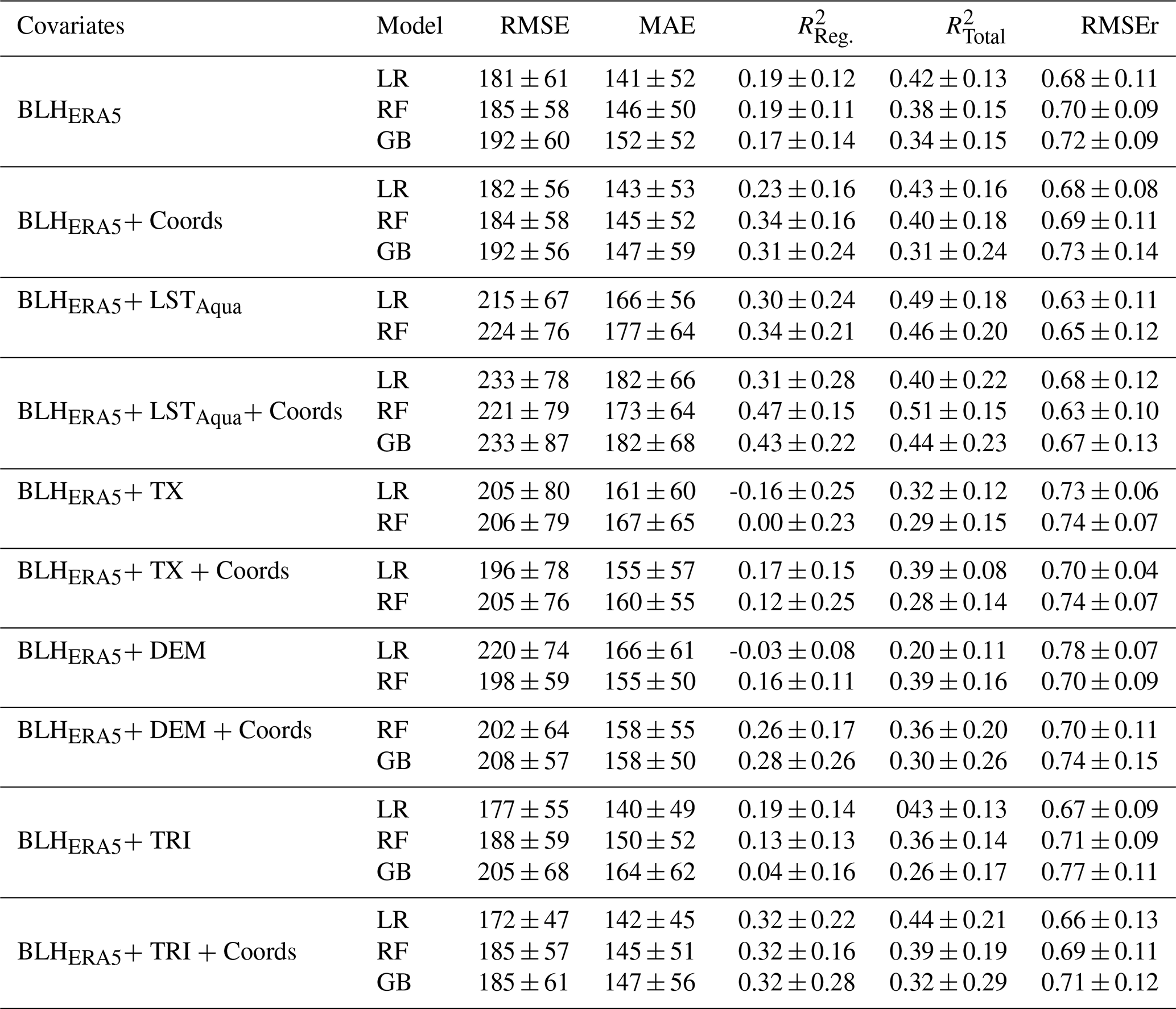
The incorporation of kriging improved model performance by between 10 % and 20 %. However, two distinct patterns were observed: 1 – kriging enhanced the final fit in cases where the regressions had negative mean values, as was the case for the TX and DEM combinations. 2 – Kriging contribution was negligible in the case of GB (e.g., BLH_ERA5+ Coords or BLH_ERA5+ TRI + Coords), where the incorporation of the spatial component did not result in substantial enhancements.

Among the variables evaluated and their different combinations, FG was the variable that presented the greatest difficulties for modelling. This was evidenced by the low R² (data not shown). Consequently, this variable was excluded from the subsequent analysis at 12:00 UTC. Therefore, for the testing section at 12:00 UTC, the models that exhibited the best values were selected (e.g., RMSEr ≤0.70): BHL_ERA5+ LST_Aqua + Coords using RF, ERA5 + Coords (LR), BLH_ERA5+ TRI + Coords (LR) and BLH_ERA5+ DEM (RF).

At 00:00 UTC, the kriging part did not improve the BLH_RS prediction, therefore only the regression was considered. Additionally, the models were unable to consistently reproduce the observed values for the twelve-month data (for example March, April, May, October and November obtained R²<0 with any model combination). However, when the results were analysed on a seasonal basis, acceptable fits were obtained during two contrasting season (Table 3), winter (December, January and February) and summer (June, July and August). During the summer period, the GB model using BLH_ERA5 and LST as input variables was the only approach achieving a meaningful predictive performance (R²>0). In contrast, during the winter months, five models were retained, although these models exhibited weak predictive skill, with R² values ranging from 0.06 to 0.16. Combinations that included TG, FG, TRI and DEM did not achieve satisfactory levels of fit and were discarded at night.

Therefore, for testing section at 00:00 UTC the following model were considered for winter data: BLH_ERA5+ LST_Terra combination using LR, BLH_ERA5 (RF), and BLH_ERA5+ LST_Terra+ Coords (RF). Finally, the BLH_ERA5+ LST_Terra model with GB was considered for summer.

3.2 Interpolation testing

3.2.1 Spatial testing

As shown in Fig. 2a, at 12:00 UTC the predicted four models performed closer to the observations during the autumn, spring, and winter seasons, whereas greater discrepancies were observed during the summer. These observations were in line with the RMSE values (Table 4), during the spring-summer seasons, the models exhibit an RMSE ≥ 125 m. In contrast, during winter and autumn the RMSE values tend to decrease. Moreover, the ERA5_blh values deviated the most from observations in all seasons, with a 250 m < RMSE < 470 m. Overall, the best models were BLH_ERA5+ Coords (LR) in summer, BLH_ERA5+ TRI + Coords in spring (LR) and BLH_ERA5+ DEM (RF) in winter and autumn. Showing better performance than those from ERA5_blh (Table 4, Fig. 2a).

Table 3 Mean and standard deviation of the diagnostic parameters: RMSE, MAE, R² and RMSEr obtained during the regression kriging training process at 00:00 UTC for the three regression algorithms and the different covariate combinations. In this case, the R² is reported only for the regression component ($R_{\mathrm{Reg}.}^{\mathrm{2}}$). LR = Linear Regression; RF = Random Forest; GB = Gradient Boosting.

Table 4 Root mean square error (RMSE, m) between observed values (BLH_RS), ERA5_blh, and model estimates sorted by climatic season, using an independent dataset (13 stations at 12:00 UTC and 10 stations at 00:00 UTC). Regression models used in the deterministic component are indicated in parentheses: LR = Linear Regression; RF = Random Forest; GB = Gradient Boosting.

During the winter season, the interpolation models evaluated at 00:00 UTC showed comparable performance, with RMSE values ranging from approximately 75 to 93 m (Table 4). All models exhibited a tendency to underestimate the observed BLH values, as shown in Fig. 2b, with the RF model using only BLH_ERA5 as input showing the largest deviations. In contrast, during summer, the BLH_ERA5+ LST_Terra model (GB) showed the best agreement with observations, achieving an RMSE below 15 m. Finally, ERA5_blh consistently overestimated the observed values, with RMSE values ranging between 63 and 97 m.

Figure 2 Boxplot of boundary-layer height from observation (BLH_RS), Copernicus (ERA5_blh), and from the interpolation models divided by seasons (2010–2020 years). (a) 12:00 UTC and (b) 00:00 UTC. Regression model in brackets. The boxes in each season/ hour are colour-coded according to the legend on the right side. The solid black line shows the median, and the white circles the mean values. The whiskers extend to the 5th and 95th percentiles. Grey circles beyond or above the whiskers show the outliers.

3.2.2 Temporal testing

In this section, seasonal mean BLH_RS values (2021–2024 period) were compared with ERA5_blh from the same period, as well as with estimates from models trained on the 2010–2020 dataset.

At 12:00 UTC, the interpolated estimates were closest to the observations in all seasons, only in winter, the model with LST (RMSE = 147 m; Table 5) was different from observed values (Fig. 3a). Predictions were more biased during the warmest months (e.g., RMSE ∼ 230 m), while in winter and autumn, RMSE values ranged between 103 to 179 m. In addition, as previously observed in Fig. 2, ERA5_blh systematically overestimated the observed values across all seasons, with RMSE values ranging from 235 to 346 m (Table 5).

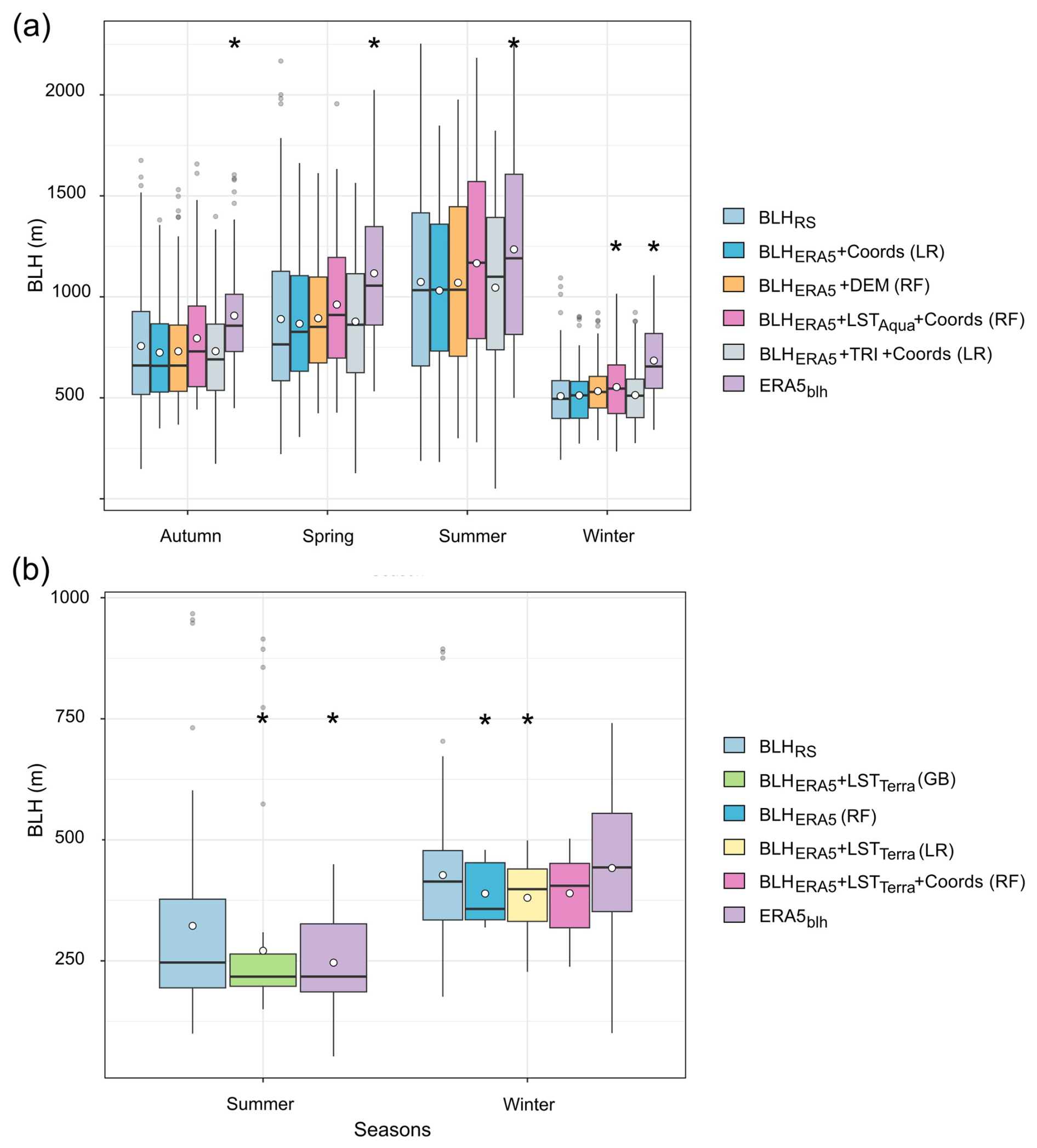
Figure 3 Boxplot of boundary-layer height from observation (BLH_RS, 2021–2024 years), Copernicus (ERA5_blh, 2021–2024 years), and from the interpolation models (2010–2020 years), divided by seasons. (a) 12:00 UTC and (b) 00:00 UTC. Significant differences (p<0.05) with BLH_RS values were indicated by *. Other references in Fig. 2.

Table 5 Root mean square error (RMSE, m) between observed values (BLH_RS; 2021–2024 years), model estimates (2010–2020 years), and ERA5_blh (2021–2024 years), sorted by climatic season. Regression models used in the deterministic component are indicated in parentheses: LR = Linear Regression; RF = Random Forest; GB = Gradient Boosting. By season, we had 34 stations at 12:00 UTC and 23 stations at 00:00 UTC.

At 00:00 UTC (Fig. 3b), during winter, the best-performing model was BLH_ERA5+ LST_Terra+ Coords (RF), with an RMSE of 162 m, followed by ERA5_blh, with an RMSE of 202 m (Table 5). In contrast, during summer, both the interpolation model and ERA5_blh showed a reduction in accuracy. However, the regression model BLH_ERA5 + LST_Terra (GB) still achieved a lower RMSE than ERA5_blh (Table 5).

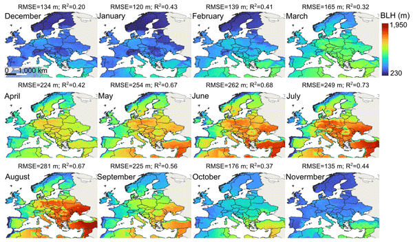
The RF model using BLH_ERA5+ DEM was selected to represent BLH over the study area at 12:00 UTC, as it consistently showed the closest agreement with observed values during both spatial and temporal validation, achieving RMSE values below 230 m. In Fig. 4 the monthly BLH in metres at 12:00 UTC was spatially represented. A clear seasonal pattern can be observed: the lowest values are recorded during the autumn-winter period, whilst the highest correspond to spring-summer. This same seasonal pattern is reflected in the RMSE (calculated using the training data), which is lower in the colder months and higher in the warmer months. Meanwhile, the coefficient of determination (R²) has lower values in autumn and winter and higher values in spring and summer.

During the night, it was not possible to achieve a comparable level of monthly representativeness. The models tested (during winter and summer) were not consistent in their estimation of the BLH at night; it was therefore decided to exclude their representation from the final analysis.

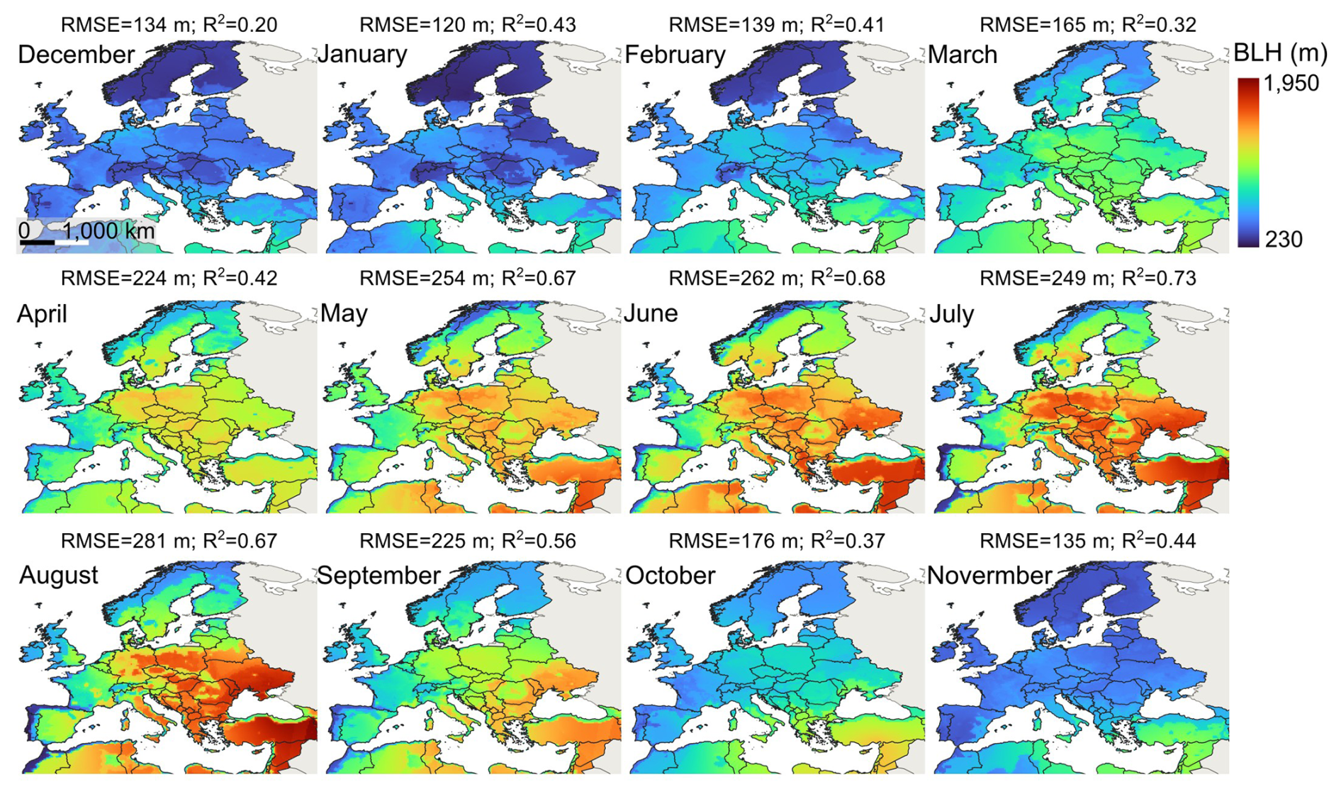
Figure 4 Monthly gridded maps of boundary layer height obtained with Regression Kriging over Europe at 12:00 UTC (2010–2020), with BLH_ERA5 + DEM (RF) as covariates. Monthly mean of RMSE and $R_{\mathrm{Total}}^{\mathrm{2}}$ for training are shown in the upper part of the gridded maps.

4 Discussion

In the present study we model the planetary boundary layer combining different data sources using the regression kriging framework. Our main finding was the higher spatio-temporal accuracy achieved in comparison with another widely used and validated product, namely the ERA5 reanalysis.

The distinct stages in the dynamics of the planetary boundary layer were reflected in the differences in model performance between midday (12:00 UTC) and midnight (00:00 UTC). The results at midday showed better performance than those obtained at night. In both cases, however, combining reanalysis, coordinates and LST covariates, and Linear Regression and Random Forest provided the best representation of the observed values.

Obtaining reliable and accurate models during nighttime conditions proved to be a major challenge, whereas during daytime, the monthly planetary boundary layer height could be reconstructed over the European region with an error below 250 m. Furthermore, a seasonal pattern was identified, whereby the RMSE and interquartile range exhibited a higher value during the warmer months in comparison to the colder months.

The following sections discuss the proposed methodology, the most relevant covariates and their relationship with the planetary boundary layer, the seasonal performances and testing result.

4.1 Interpolation method

Recently, several studies have employed machine learning models to estimate or predict the planetary boundary layer. For instance, Ayazpour et al. (2023) produced a gridded map across the USA using eXtreme Gradient Boosting, improving the estimated BLH values in some cases (RMSE >200 m) compared to reanalysis BLH data (e.g., ERA5, MERRA, and NARR). In a global-scale study, Guo et al. (2024) estimated the differences (bias) between BLH obtained from radiosondes and ERA5 using Random Forest regression alongside climatic and physical variables. They obtained a corrected BLH value which, when compared with radiosonde BLH, yielded a mean absolute bias of 168 m. Then, Zhang et al. (2025), at an atmospheric observatory in Oklahoma (USA), modelled BLH values at 10 min intervals using three ML algorithms; The best-performing model achieved an RMSE of approximately 110 m stable and 240 m for unstable BL. Finally, Stapleton et al. (2025) employed ceilometer data from two sites in Central Amazonia, utilising distinct machine learning approaches to model the BLH. They found that Light Gradient Boosting model was the most effective model, achieving a 310 > RMSE > 200 m for daytime and 140 > RMSE > 200 m for night-time. Notwithstanding the methodological differences, sample sizes, and study areas, our work has yielded similar results in terms of error parameters (Tables 2, 3, 4, and 5), thereby validating the methodology applied in the present study.

We opted for regression kriging rather than others regression tools for prediction because, in RK, once the deterministic component of variation has been estimated, the residuals can be interpolated using kriging and added to the estimated trend. Therefore, if there is a strong correlation between the target variable and the covariates (linear or not), the residuals are small or close to zero, and the prediction relies on the regression model. Conversely, if there is no strong correlation between the variables, the prediction depends on the spatial autocorrelation of the residuals (Hengl et al., 2007). The results obtained in this study are consistent with these ideas, as shown in Table 2, which indicates that the coefficient of determination improves when kriging is applied to the regression residuals. This behaviour had previously been documented by Zhu et al. (2022) in China, who, in a study that modelled soil organic carbon concentration using various machine learning-based regression models and complementing these with kriging, found that the regression-kriging approach outperformed purely regression-based models in terms of accuracy. This improvement was closely linked to the spatial dependence of the response variable, an aspect that machine learning models often overlook (Takoutsing and Heuvelink, 2022). However, when this spatial autocorrelation is negligible or when the model assumptions are not met, the contribution of kriging decreases dramatically, as evidenced by the results obtained during the night (Table 3), and with some covariates.

In contrast to classical models such as linear regression, regression models based on machine learning do not require strict distributional assumptions to be met, making them considerably more effective at modelling the planetary boundary layer both during the day and at night. However, the differences between them were less than 50 m (Tables 4 and 5). It is important to acknowledge the limitations of the regression-kriging technique. Including the use of low-quality data (for both the response variable and the covariates), an insufficient sample size, poor estimation of the spatial model, extrapolation beyond the observed range, the use of predictors that do not maintain a stable relationship with the target variable, and the risk of model overfitting (Hengl, 2009).

Despite these limitations mentioned above, the results obtained using the proposed methodology were favourable, compared with other studies (as mentioned above) and particularly when compared with the ERA5 reanalysis values. Moreover, rather than RMSEr values being close to 0.7, the interpolation models still performed better than the ERA5 data available for the same locations (e.g., Tables 4 and 5; Figs. 2 and 3).

These findings suggest the possibility of using ERA5 data to obtain more accurate estimates of the boundary layer height, as previously demonstrated by Ayazpour et al. (2023) and Guo et al. (2024). We believe that by improving spatial representation-that is, by increasing the number of weather stations-and by enhancing the quality of the input data (both the dependent variable and the covariates), this methodology could provide even more accurate estimates of the BLH. However, these claims should be treated with caution, as the ERA5 reanalysis BLH data have limitations, which will be discussed in the following section.

4.2 Relevance of covariates

The combination of the land surface temperature and Coords with BLH_ERA5 values provides the most favourable prediction of planetary boundary layer data at both times considered. At 12:00 UTC, topography (TRI and DEM) can also be used. Nevertheless, this relevance is overshadowed by the large dispersion of the results (Figs. 2 and 3). This data spread could be related to the sampling and structural uncertainties associated with the method (Sinclair et al., 2022), which can amount to several hundred metres, up to 1 km (Seidel et al., 2010). This introduces an intrinsic variability in the BLH_RS data (used as targets), which is subsequently reflected in our results.

4.2.1 ERA5 reanalysis

The relevance of ERA5 as covariate (BLH_ERA) is not unexpected, due to corresponds to the target variable, derived from ECMWF data assimilation, which has previously been reported to show good accuracy when compared with radiosonde observations (Guo et al., 2021; Li et al., 2023; Xu et al., 2023). However, our results show marked differences between the models obtained for the midday (12:00 UTC) and those developed for the night (00:00 UTC). Moreover, although the correlation coefficient was 0.8 between radiosonde and BLH_ERA5 values at 00:00 UTC (Table 1), the diagnostic parameters evaluated showed that BLH_ERA5 explain a limited proportion of the variability observed in the radiosonde measurements (R²∼0.1, Table 3). Consequently, the implementation of a methodological framework in two opposing phases of the atmospheric boundary layer is subject to limitations.

A plethora of studies have documented discrepancies in the performance of the ERA5 reanalysis in representing the BLH under stable and unstable atmospheric conditions. For instance, Seidel et al. (2012) conducted an analysis of the climatology of the BLH over Europe and the United States using radiosonde observations, when comparing observations with values obtained from ERA5-Interim, they found that the reanalysis struggles to adequately represent the BLH under unstable atmospheric conditions. This is a challenge that the advances in the ERA5 reanalysis have not managed to overcome; other studies have reached the same conclusion. For instance, Sinclair et al. (2022) investigated the BLH in southern Finland using radiosonde observations and ERA5 reanalysis data. They found good agreement between ERA5 and the observations under unstable atmospheric conditions; however, the accuracy of the reanalysis decreased under stable conditions, where ERA5 tended to overestimate BLH values. In China, Xu et al. (2023) obtained similar result, e.g., they found good agreement between ERA5 the convective layer and the neutral layer obtained by radiosondes. However, under stable boundary layer conditions, ERA5 showed again a marked overestimation of the BLH. This outcome may be associated with several factors, such as differences in the calculation of the Richardson number, or the coarse vertical resolution in ERA5 compared with radiosondes, and other possible factors have been previously discussed in other works (Seidel et al., 2010; Guo et al., 2021, 2024; Madonna et al., 2021; Dias-Júnior et al., 2022; Sinclair et al., 2022; Slättberg et al., 2022; Xu et al., 2023; etc.).

4.2.2 Topography

Several studies have reported reduced performance of the ERA5 reanalysis product in regions with complex topography, e.g., for climatic variables (Cavalleri et al., 2024; Crespi et al., 2024) and boundary layer height (Guo et al., 2021, 2024). This may be because coarse-scale resolutions (∼25 km²) fail to capture the processes occurring at a smaller scale, such as landscape heterogeneity (Guo et al., 2021; Slättberg et al., 2022). This may explain why including DEM and TRI in high resolution could improve the prediction of observed values.

On average, the weather stations were located at an altitude of 150 m a.s.l. (range: 0–627 m), whilst the TRI ranged from 2 to 1100 m. Altitude and terrain roughness are indirect indicators of topographical variability, such as valleys, slopes and plateaus. Together, they influence the dynamics of air mass flows, resulting in significantly different boundary layer dynamics in mountainous areas compared to flat terrain. During daytime fair-weather conditions, solar radiation generates thermally induced upslope winds and turbulent convection, which generally cause the BL to grow. However, the grow is not spatially uniform, it initiates first over mountain tops, where nighttime cold-air drainage prevents the formation of strong inversions, allowing rapid heating and early BL development. In contrast, the BL growth over valley floors is delayed due to the presence of a nocturnal cold-air pool and a strong surface-based inversion, in the afternoon BL growth in the valleys accelerates and may catch up with the ridges. During the night, radiative cooling at the surface generates downslope and down-valley winds, leading to the formation of a shallow and stable boundary layer, typically only on the order of 100 m in depth (De Wekker and Kossmann 2015).

The TRI and DEM variables provided a better fit to 12:00 UTC than at 00:00 UTC dataset. We attribute this time difference to two sources of uncertainty. Firstly, the well-known difficulty of the ERA5 model in estimating the height of the boundary layer at night, as discussed in the previous section. Secondly, the specific characteristics of the nocturnal boundary layer in valleys, considering that in general the European stations in mountainous areas are in valleys (Seidel et al., 2012). The combination of an extremely low and stable boundary layer in valley and the reduced accuracy of measurement instruments in complex terrains (De Wekker and Kossmann 2015) could explain the greater discrepancy observed between both UTC.

4.2.3 Coordinates

The use of geographical coordinates as covariates is an effective approach when combined with BLH_ERA5 and LST, as it considers the significant influence of geographic location on the development of the planetary boundary layer. For example, latitude is associated with the amount of solar radiation reaching the Earth's surface. In lower latitudes, the land surface receives more solar radiation, resulting in deeper BLH (Guo et al., 2021). Consequently, as we move away from the equator, the incoming solar radiation per unit area decreases (Stull, 1988), explaining the negative correlations with BLH_RS (Table 1). Conversely, longitude is directly related to local solar time. Therefore, at the same UTC, the stations located on the western side of the study area (∼ UTC −1, 0) receive less time exposure of sunlight than those on the eastern edge (∼ UTC +1, +2) (Seidel et al., 2012; Guo et al., 2021).

4.2.4 Land Surface Temperature

The relationship between temperature and the BLH is governed by turbulence. During the day, surface heating increases buoyancy, generating turbulence that causes warm air masses to rise. This process, together with the entrainment of air from the free atmosphere, causes the BL to grow vertically more than 1 km. Conversely, at night, the cooling of the ground suppresses buoyancy and even dissipates it, stabilising the atmosphere. The BL then collapses to a few hundred metres, and the residual turbulence that persists is of mechanical origin, generated by wind shear near the surface, but with an intensity far lower than that of diurnal convective turbulence (Teixeira et al., 2021).

Temperature variables from MODIS (LST) and E-OBS (TG and TX) exhibited moderate correlations with the BLH at both UTC (r∼0.70), albeit with opposite signs (Table 1), which is consistent with the anti-correlation between diurnal and nocturnal BLH (Seidel et al., 2012). However, LST explained slightly better the proportion of the variability in BLH than the TX at midday, and TG at night. This difference may be related to the fact that MODIS data represent smaller spatial areas (∼1 vs. ∼10 km²), providing a more local characterisation of surface radiation conditions (heating). Furthermore, LST corresponds to a specific daily observation, whilst TG represents an average daily temperature, which could attenuate part of the variable relevance. It is noteworthy that TX demonstrated reasonable performance at 12:00 UTC (Table 2); nevertheless, its explanatory power was inferior in comparison to LST. The difference between atmospheric and land surface temperature is the main driver of the sensible heat flux from the surface (Monteith, 1981). However, since LST has generally a wider diurnal range with respect to air temperature (Zhang et al., 2014), it is then likely that it serves as a more sensitive predictor for BLH.

4.2.5 Covariates limitation

When air temperature and wind speed were considered in our models, these climatic variables were far from reaching the level of relevance we had expected. According to the literature, an increase in surface temperature or wind speed is generally associated with greater development of the BLH (Seidel et al., 2012; Guo et al., 2016; Li et al., 2023). However, in other studies, wind speed (Ayazpour et al., 2023; Zhang et al., 2025) and air temperature (Zhang et al., 2025) have been excluded from BLH modelling due to their low relevance in regression-based models.

It is worth mentioning that several limitations in the covariate datasets used may have directly influenced our results and its application in RK. (a) The available LST values. Only clear-sky days were considered, which may have led to higher BL development, since there is a direct relationship between clear-sky, without clouds, conditions and BL growth, and consequently its height (Quan et al., 2013; Guo et al., 2016). Moreover, this restriction reduced the number of daily values per station. This influenced the monthly means used in the interpolation and ultimately affected the realistic representation of the BL. (b) Station density. The E-OBS variables (TX, TG, and FG) were represented by a relatively low station density, mainly due to spatial cover limitations. It is well known that low spatial density directly affects the accuracy of the interpolation methods (Krähenmann et al., 2018; Argañaraz et al., 2025). (c) Data inhomogeneity. Although the E-OBS dataset has been regularly updated since 1950, it still presents uneven station coverage across Europe. Variations in data density over time, together with inconsistencies in the observation records, may influence the representation of long-term climate variability in the gridded datasets (Crespi et al., 2024).

Finally, we can mention the relevance of the coarse resolution. 1 – Temporal, another important aspect concerns the daily and effectively 24 h temporal resolution of the E-OBS variables (TG, TX, and FG). This inevitably introduces bias, as the same gridded values must be used for both synoptic hours. Consequently, these inputs resemble broad daily averages rather than precise time-specific measurements 2 – Spatial, the variables represented at a finer resolution (for example, LST with 1 km² spatial resolution, altitude and TRI at 10 m², and latitude and longitude coordinates with three decimal places) demonstrated very good performance in comparison with variables with a coarser spatial scale, such as E-OBS (∼10 km² resolution). These results suggest that processes associated with smaller spatial scales may play a significant role in the development and variability of the atmospheric boundary layer (Stapleton et al., 2025).

4.3 Seasonal performance and testing

The planetary boundary layer exhibits a pronounced diurnal cycle, with its height varying from only a few tens of metres at night to over one kilometre during the day, and with different levels of uncertainty associated with these measurements (Seidel et al., 2012; Guo et al., 2021). Despite the limitations related to the number of available stations, our results were consistent with previously reported patterns for the European region, showing higher BLH values in summer during the day, and in winter during the night (Figs. 2 and 3) (Seidel et al., 2012). Moreover, for both validation approaches, we found higher RMSE values during the warm seasons than during the cold seasons, with this contrast being more pronounced during daytime than at night (Tables 4 and 5). This finding is consistent with Guo et al. (2021), who reported a similar seasonal pattern at the global scale, based on bias values between observations and four different reanalysis products.

During spatial testing, the models' values were closer to the observed values at both UTC, while ERA5_blh were, on average, higher than the observed values (Fig. 2). This tendency to overestimate the values obtained from radiosondes has already been mentioned in other studies (Zhang et al., 2020; Sinclair et al., 2022). Additionally, in the temporal testing at 12:00 UTC, significant differences were detected among the interpolation models and reanalysis, being the interpolation models more accurately than ERA5_blh values. It is important to note that ERA5_blh values share the same temporal scale as the observation (BLH_RS) data. Consequently, this highlighted the performance of the interpolation models, which were developed using data from the 2010–2020 period.

This finding was contrasted at night, where the ERA5_blh were similar to the observations in the coldest seasons, whereas the interpolation models lost precision in summer and in winter, only the combination with temperature and coords was close to observation (Fig. 3b). However, the models exhibited lower RMSE values than ERA5_blh. Although this may seem contradictory, it can be explained by the higher dispersion of ERA5_blh values compared with the models, as reflected by the elongated boxplots in Fig. 3b. This highlights a limitation in predicting BLH at night, as was previously discussed.

This limitation to modelling the BLH at night is not exclusive to our interpolation models; previously, several authors have reported it for reanalysis products (Seidel et al., 2012; Sinclair et al., 2022; Xu et al., 2023), BLH estimates derived from lidar observations (Zhang et al., 2025), and radiosonde measurements (Gu et al., 2020).

5 Conclusions

In this study, we implemented a classic technique, such as regression kriging, to obtain gridded maps of the planetary boundary layer height, integrating multiple data sources. The approach, despite its limitations at night, yielded good spatial and temporal accuracy compared with the ERA5 reanalysis.

The combination of reanalysis ERA5 with high resolution land surface temperature, topographic (DEM and TRI) and coordinates covariates, provided the most accurate estimates to boundary layer height. Moreover, reflecting the inherent complexity of the boundary layer, the machine-learning regression methods outperformed linear regression.

Model performance differed between midday and midnight. In the spatial validation, both during the day and at night, the interpolation models provided a closer approximation to the observed values than ERA5_blh. During the temporal validation, the interpolation models were more accurate during daytime than ERA5_blh and exhibited reduced accuracy at night. Overall, the main limitations were observed during nighttime.

Our results highlight the potential of simple tools such as regression kriging to generate gridded maps that provide improved approximations of the 12:00 UTC boundary layer in known and new areas and more limited approximations of the stable boundary layer at 00:00 UTC at new areas. Considering that our study is based on a limited number of stations, we strongly believe that the performance of this interpolation method could be substantially improved with a denser coverage of meteorological stations, potentially yielding better results than those obtained here and enhancing those from currently available reanalysis products.

Appendix A:  

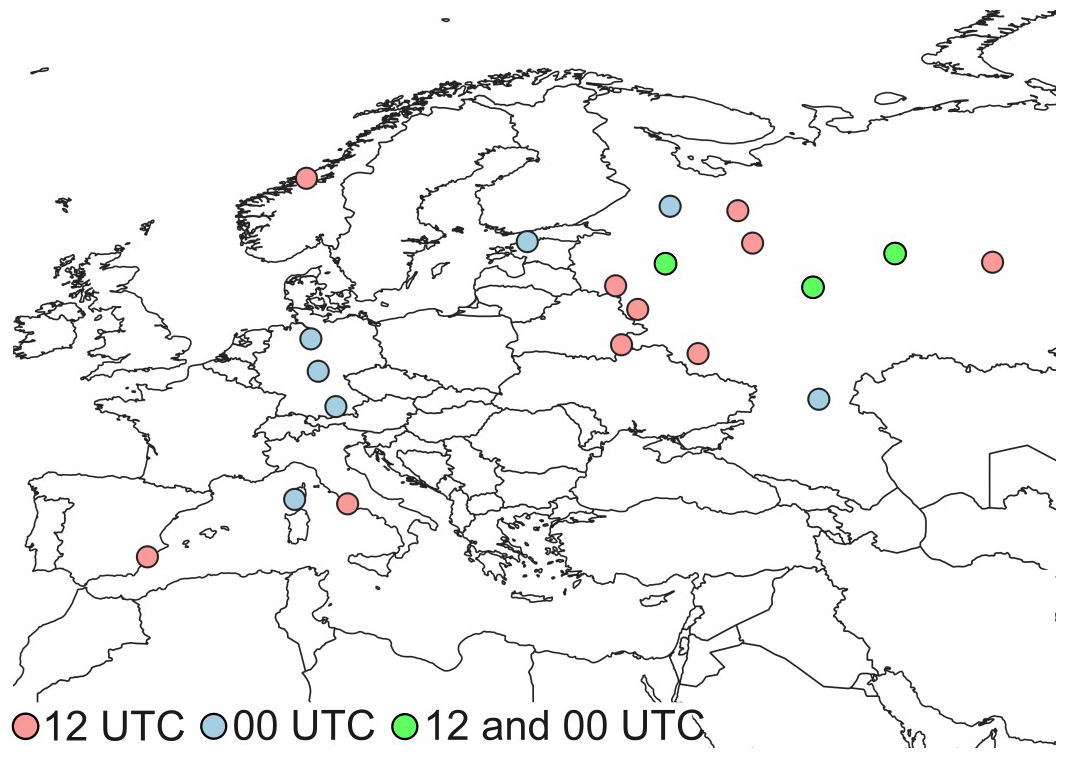
Figure A1 Spatial distribution of stations used for spatial validation. References are provided in the figure.

Figure A2 Root mean square error (RMSE) for each temperature variable comparison at each time by month. Although the differences were not statistically significant in all cases, TX and LST_Aqua showed lower error values at 12:00 UTC (a), while TG and LST_Terra performed better at 00:00 UTC (b).