Measurement of turbulence energy dissipation rate by a standalone high-resolution Doppler lidar

A second-order structure-function model for lidar line-of-sight (LOS) velocities is proposed. This structure-function model corrects for turbulence filtering caused by probe volume averaging using a Gaussian weighting function. The structure function model corrects for both spatial and temporal averaging effects. It takes advantage of the high range gate resolution of the BEAM 6x pulsed lidar used in this study, i.e., 3 m, to effectively resolve the inertial subrange. The structure function model is then used to obtain the turbulence energy dissipation rate (ε) by fitting it to lidar measurements in the inertial subrange. Unlike previously presented structure-function methods for evaluating ε in the literature, this method has a weaker dependence on the turbulence length scale. The estimated ε values from the lidar are compared with those from ultrasonic anemometers at three heights: 103, 175, and 241 m. The comparison results show an excellent correlation between the two sets, with a Pearson correlation coefficient (ρ) exceeding 0.9 across all three heights. The observed bias was also very small: more than 50 % of all lidar-measured ε values were within ±20 % of the sonic-measured values. This method relies on accurate detection of the inertial subrange; hence, under very stable atmospheric conditions, the model fit to the measurements produced relatively large errors due to the difficulty of detecting the inertial subrange. Applications of this method include, but are not limited to, quantifying turbulence in the wake of aircraft, understanding pollutant dispersion in urban environments, and assessing wind resources and turbulence in areas or at heights where erecting a meteorological mast is not possible.

1 Introduction

Turbulence measurements hold paramount significance in atmospheric sciences and renewable energy applications. These measurements are used to understand and quantify aerosols, heat, moisture, and momentum in the atmospheric boundary layer (Stull, 1988). In the troposphere, turbulence governs energy and momentum exchange between the Earth's surface and the air above it. Turbulence measurements are also used to monitor and understand air quality, pollutant dispersion, and heat dynamics in urban meteorology. Atmospheric turbulence is usually measured with in situ instruments, such as sonic anemometers, that can be installed on a meteorological mast. These instruments measure turbulence at a fixed point in space. Erecting a meteorological mast for turbulence measurements may not always be feasible, especially in complex terrain, deep offshore seas, or in conditions where in situ measurements are not possible, e.g., aircraft wake vortices. In such cases, remote sensing devices such as Doppler wind lidars can be used to estimate atmospheric turbulence. Commercial scanning lidars also provide the capability to get multi-point statistics and vertical profiles, thus presenting a more detailed view of the atmosphere.

Estimating turbulence from a Doppler wind lidar is not a novel concept. There are two key challenges associated with it, as delineated by Peña et al. (2025): turbulence contamination and probe-volume averaging. The former arises from reconstructing wind velocity components from lidar line-of-sight (LOS) velocities, while the latter is inherent to the measuring principle of Doppler lidars, which do not record point measurements; rather, they measure within a probe volume, acting as a turbulence filter. A number of methods and scanning strategies have been proposed to operate Doppler lidars as standalone instruments for measuring atmospheric turbulence. Eberhard et al. (1989) used a short-pulse Doppler wind lidar with a range gate resolution of 150 m to measure Reynolds stresses and turbulence kinetic energy (TKE) profiles in the atmosphere. Their method relies on the conical scanning of the atmosphere at a fixed elevation angle and deducing Reynolds stress values directly from the individual beam LOS variances. This approach avoids cross-contamination among the wind field components; however, it does not address turbulence filtering due to probe volume averaging (Bonin et al., 2017; Sathe and Mann, 2013). This method has been further improved and optimized for a Doppler beam swing (DBS) scanning pattern, where only five azimuth measurements at a fixed elevation angle and one vertical measurement are obtained to deduce the full Reynolds stress tensor (Sathe et al., 2015).

A significant amount of research efforts has been made to address the turbulence filtering or the attenuation of small-scale turbulence due to probe-volume averaging. Frehlich et al. (1998) and Frehlich and Cornman (2002) utilized the LOS velocity structure function (D(r), where r is the separation distance) for a pulsed lidar to estimate the turbulence energy dissipation rate ε. They removed the effect of spatial averaging using theoretical corrections, such as modeling the lidar range weighting as a Gaussian function. In this approach, the measured second-order structure function is fitted to a theoretical D(r) model that accounts for the probe-volume averaging of the lidar LOS velocities. Smalikho et al. (2005) obtained ε from the longitudinal structure function of LOS velocities measured by a 2 µm lidar with a range gate resolution of 30 m and compared it with the ε estimates obtained from the Doppler spectrum width (DSW) method, confirming the results with numerical simulations. Their results showed a high correlation between the two methods and a reduction in bias as ε increased. Smalikho and Banakh (2017) and Wildmann et al. (2020) utilized the azimuthal structure function of LOS velocities obtained from the conically scanning vertical profiling lidars to estimate ε and TKE. Both studies account for the probe volume averaging by defining a transverse filter function. However, the latter introduced an additional advection filter to account for turbulence advection within the scanning plane. The ε estimates were then compared with the sonic anemometers. Correcting for advection reduced the bias; however, the random error, as indicated by the observed scatter, remained relatively high.

A major drawback of these methods is that the presented D(r) models are also dependent on the outer scale of turbulence ℒ_o. To obtain ℒ_o, it was often assumed that the large-scale turbulence is isotropic and can be modeled by an isotropic spectral model, such as the von Kármán spectral model. However, the von Kármán spectral model applies only to special cases of isotropic, homogeneous turbulence. In reality, the atmospheric turbulence is highly anisotropic (Mann, 1994; Kaimal and Finnigan, 1994). In order to find ε from such methods, the modeled D(r) was fitted to the measurements in such a way that the best fitting takes place for both variables: ε and ℒ_o (Frehlich and Cornman, 2002; Frehlich et al., 1998; Smalikho et al., 2005). The best fit obtained using this method may not provide the best ε value, since ℒ_o is also being fitted to minimize the error function. Any anisotropy in the large-scale turbulence would distort ε estimates. Furthermore, it unnecessarily complicates the fitting procedure as more than one variable is involved.

Turbulence energy dissipation rate can also be obtained through the one-dimensional LOS velocity spectrum, provided that the inertial sub-range is detected (Davis et al., 2008; O'Connor et al., 2010; Bodini et al., 2018; Wildmann et al., 2019). However, this method requires invoking Taylor's hypothesis of frozen turbulence (Taylor, 1935) and a suitable choice of ℒ_o. The effect of turbulence filtering due to probe volume averaging was also modeled to obtain the corrected velocity spectrum, thereby improving the prediction of ε (Banakh and Smalikho, 1997; Drobinski et al., 2000). In summary, there are two primary ways of estimating ε from the Doppler lidar measurements reported in the scientific literature: the structure function method and the velocity spectrum method. Both these methods usually require knowledge about the outer scale of turbulence, ℒ_o, and may invoke the assumption of frozen turbulence.

In this article, we present an improved second-order longitudinal structure function model for lidar LOS velocities that also accounts for probe volume averaging in a pulsed lidar. The presented structure function model improves on the previously described methods in the following two ways: (i) the lidar system used in this study provides LOS velocity estimates at closely spaced range gates, with a range-gate spacing of 3 m along the beam. Such a small range-gate spacing enables evaluation of the structure function D(r) at small separations, thereby improving the identification of the inertial subrange. and (ii) the use of longitudinal D(r) means that there is no need to assume Taylor's frozen turbulence hypothesis, as all the LOS measurements along the lidar beam have a known constant separation distance r between the range gates. This ensures that the structure function model only depends on ε in the inertial subrange. The model is then used to estimate the turbulence energy dissipation rate ε in the atmospheric boundary layer, and the values are validated against sonic anemometer measurements at three heights of 103, 175, and 241 m above ground level at a test site in Denmark.

The second-order longitudinal structure function model for lidar LOS velocities is presented in detail in Sect. 2. In Sect. 3, the test site and information about the lidar and the validation data (ultrasonic anemometers) are provided. Section 4 presents the complete workflow for estimating ε from ultrasonic anemometer and lidar data. Section 5 describes the validation of lidar-derived ε estimates against sonic anemometer data and the relevant discussion. Section 6 concludes the article by describing the salient features of the model and summarizing the study's significant results.

2 Second-order structure function model for lidar line-of-sight velocities

The second-order velocity structure function is the variance of the difference in velocity between two points x and x+r, where r is the separation vector between them. The second-order structure function can be defined as:

$$\begin{array}{}\text{(1)}& D\left(r\right)=〈{\left[\mathit{n}\cdot \mathit{v}\left(\mathit{x}\right)-\mathit{n}\cdot \mathit{v}(\mathit{x}+\mathit{r})\right]}^{\mathrm{2}}〉,\end{array}$$

where $\mathit{n}=\mathit{r}/\left|\mathit{r}\right|$. Since the component n⋅v of the velocity vector is aligned with n, this is called a longitudinal structure function. Kolmogorov (Pope, 2000) hypothesized that in the inertial subrange, the turbulence is locally isotropic and D(r) is only a function of the turbulent energy dissipation rate ε, the separation distance r, and the universal Kolmogorov constant C_K≈2. Hence, for $\left|\mathit{r}\right|\ll {\mathcal{L}}_{\mathrm{o}}$, where ℒ_o is the integral length scale or the size of the largest eddies,

$$\begin{array}{}\text{(2)}& D\left(r\right)=C_{\mathrm{K}}(\mathit{\epsilon }r{)}^{\mathrm{2}/\mathrm{3}}.\end{array}$$

The pulsed Doppler lidar measures backscattered light over a finite spatial volume, so-called probe volume, the extent of which is governed by the pulse duration. The return signal, therefore, contains contributions from the aerosol particles distributed throughout the probe volume. The center of the probe volume is typically assigned as the nominal range gate position and determined from the pulse time-of-flight (Peña and Hasager, 2011). Volume measurement is inherently different from point measurements used in reference instruments, such as sonic or cup anemometers.

The lidar used in this study measures LOS velocities at several range gates along the beam. Lidar manufacturers use various methods to estimate the representative LOS velocity from the Doppler spectrum. Following Held and Mann (2018), if we assume that the effect of probe volume on turbulence attenuation can be modeled by the centroid method of determining the dominant frequency in the Doppler spectrum, then the line-of-sight velocity of the lidar beam can be defined as:

$$\begin{array}{}\text{(3)}& v_r\left(\mathit{x}\right)=\underset{-\mathrm{\infty }}{\overset{\mathrm{\infty }}{\int }}\mathit{\phi }\left(s\right)\mathit{n}\cdot \mathit{v}(s\mathit{n}+\mathit{x})\mathrm{d}s,\end{array}$$

where n is a unit vector along the beam direction, x is the center of the lidar measuring volume at the point of interest, and s is the distance along the beam from the point x. φ(s) is the weighting function normalized to unit integral, and a Gaussian shape is assumed here:

$$\begin{array}{}\text{(4)}& \mathit{\phi }\left(s\right)={\displaystyle \frac{\mathrm{1}}{\mathit{\sigma }\sqrt{\mathrm{2}\mathit{\pi }}}}{e}^{-\frac{s^{\mathrm{2}}}{\mathrm{2}{\mathit{\sigma }}^{\mathrm{2}}}},\end{array}$$

where σ is the standard deviation of the Gaussian distribution. Though Held and Mann (2018) defined Eq. (3) for a continuous-wave lidar system, the same can be assumed for a pulsed lidar system. Dolfi-Bouteyre et al. (2017) evaluated the accuracy of the centroid frequency estimator method with a coherent pulsed lidar system and found it to perform well in calculating both the first- and second-order moments of the Doppler spectrum. The longitudinal structure function along the beam then becomes:

$$\begin{array}{}\text{(5)}& D_{\mathrm{lidar}}\left(r\right)=〈{\left[\underset{-\mathrm{\infty }}{\overset{\mathrm{\infty }}{\int }}\left\{v(x+s)-v(x+r+s)\right\}\mathit{\phi }\left(s\right)\mathrm{d}s\right]}^{\mathrm{2}}〉,\end{array}$$

where r is the distance between two range gates along the beam and $v=\mathit{n}\cdot \mathit{v}$ is the velocity component along the beam direction as a function of distance along the beam. It is assumed that r and σ are small as compared to the turbulence length scale ℒ_o and the flow is homogeneous. This can be solved for the inertial subrange as (see Appendix A for a detailed derivation):

$$\begin{array}{}\text{(6)}& \begin{array}{rl}{D}_{\mathrm{lidar}}\left(r\right)=& {\displaystyle \frac{C_{\mathrm{K}}}{\sqrt{\mathit{\pi }}}}{\mathrm{2}}^{\mathrm{2}/\mathrm{3}}{\mathit{\sigma }}^{\mathrm{2}/\mathrm{3}}{\mathit{\epsilon }}^{\mathrm{2}/\mathrm{3}}\mathrm{\Gamma }\left({\displaystyle \frac{\mathrm{5}}{\mathrm{6}}}\right)\\ & \times \left\{{}_{\mathrm{1}}{F}_{\mathrm{1}}\left[-{\displaystyle \frac{\mathrm{1}}{\mathrm{3}}},{\displaystyle \frac{\mathrm{1}}{\mathrm{2}}},-{\displaystyle \frac{r^{\mathrm{2}}}{\mathrm{4}{\mathit{\sigma }}^{\mathrm{2}}}}\right]-\mathrm{1}\right\},\end{array}\end{array}$$

where Γ is the Gamma function, and ₁F₁ is the confluent hypergeometric function. The structure function model described in Eq. (6) only considers the spatial averaging and ignores any effect of temporal averaging on the lidar LOS velocities. By including the effect of the time Δt over which the lidar's Doppler signal is averaged, we can derive a modified second-order longitudinal structure function model containing both spatial and temporal averaging effects:

$$\begin{array}{}\text{(7)}& \begin{array}{rl}{D}_{\mathrm{lidar}}\left(r\right)=& {\displaystyle \frac{\mathit{\alpha }{\mathit{\epsilon }}^{\mathrm{2}/\mathrm{3}}\mathrm{\Gamma }\left(\frac{\mathrm{4}}{\mathrm{3}}\right)}{\mathrm{2}{\mathit{\pi }}^{\mathrm{1}/\mathrm{2}}\mathrm{\Gamma }\left(\frac{\mathrm{11}}{\mathrm{6}}\right)}}\underset{\mathrm{0}}{\overset{\mathrm{2}\mathit{\pi }}{\int }}\underset{\mathrm{0}}{\overset{\mathrm{\infty }}{\int }}{\mathrm{e}}^{-\left(\mathit{\sigma }\mathit{\kappa }\cos \right(\mathit{\beta }-\mathit{\theta }){)}^{\mathrm{2}}}\times \\ & \left[\mathrm{1}-\cos \left(r\mathit{\kappa }\cos \right(\mathit{\beta }-\mathit{\theta }\left)\right)\right]\\ & {\mathrm{sinc}}^{\mathrm{2}}\left({\displaystyle \frac{\mathrm{\Delta }tU\mathit{\kappa }\cos \mathit{\beta }}{\mathrm{2}}}\right)\\ & {\displaystyle \frac{\mathrm{1}-\frac{\mathrm{8}}{\mathrm{11}}{\cos }^{\mathrm{2}}(\mathit{\beta }-\mathit{\theta })}{{\mathit{\kappa }}^{\mathrm{5}/\mathrm{3}}}}\mathrm{d}\mathit{\kappa }\mathrm{d}\mathit{\beta },\end{array}\end{array}$$

where U is the mean wind speed, α is the spectral Kolmogorov constant, θ is the beam-to-wind angle measured in the plane containing both beam and wind unit vectors, and κ and β are the polar coordinates in k₁−k₂ plane (k₁ and k₂ are the along-wind and cross-wind wavenumbers). Full details on how this expression is derived are given in Appendix A.

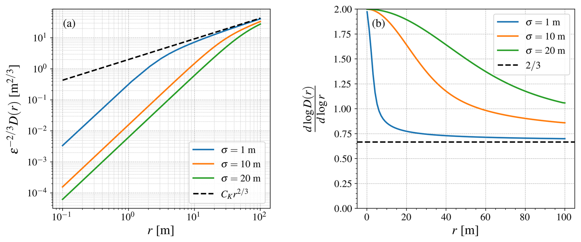
Figure 1 (a) Normalized structure function ${\mathit{\epsilon }}^{-\mathrm{2}/\mathrm{3}}{D}_{\mathrm{lidar}}\left(r\right)$ (from Eq. 6) as a function of the separation distance r for three different values of σ: 1, 10, and 20 m. A $C_{\mathrm{K}}{r}^{\mathrm{2}/\mathrm{3}}$ reference line is also added. (b) $\mathrm{d}\log D\left(r\right)/\mathrm{d}\log r$ as a function of r. The dashed black line represents a slope value of $\mathrm{2}/\mathrm{3}$.

Here we note that the lidar structure function also depends on the standard deviation of the Gaussian weighting function σ. The main assumption for accurately estimating ε is that σ should be less than ℒ_o. If atmospheric turbulence is less intense and its length scale is smaller than the lidar's sampling volume, then turbulence fluctuations will be filtered out. The choice of σ depends on the lidar instrument and can be obtained by fitting the data for a range of σ values and then selecting a value that provides the least amount of bias against true values. Figure 1a describes how D_lidar (Eq. 6) changes as a function of r for three different σ values. The change in local slope of the structure function is also a function of r, as seen in Fig. 1b. Given the measured structure function from a high-resolution lidar beam, Eq. (6) or (7) can be fitted using the least squares method or other optimization techniques to obtain the turbulence energy dissipation rate ε.

3 Data and site description

3.1 Test site

The Østerild test site is located in the northern region of Jutland, Denmark, situated between Limfjorden and Skagerrak, as shown in the inset of Fig. 2. As of 2024, the site hosts nine wind turbines for testing purposes, arranged in a north-south orientation, spanning approximately 4.7 km. Figure 2 illustrates the positions of these turbines, denoted by red dots. Each turbine is accompanied by a mast positioned approximately 2.5–4 rotor diameters to the west, with a height corresponding to the turbine's hub height. Additionally, two light masts are positioned to the north and south of the turbine row (the north mast, which is relevant for this study, is marked by a yellow dot in Fig. 2). The terrain depicted in Fig. 2 features both flat and heterogeneous characteristics, comprising a mosaic of crop and agricultural lands, urban settlements, and forested areas. Further detailed information about the Østerild site can be found in Peña (2019). For the present study, we focus only on the North mast, which is a 250 m tall mast with a triangular lattice structure. The mast is equipped with cup and ultrasonic anemometers mounted on the booms oriented at 0° from the north. The lidar pad is about 10 m west of the mast and contains the vertical profiling BEAM 6x lidar. The details about the lidar and sonic data are as follows.

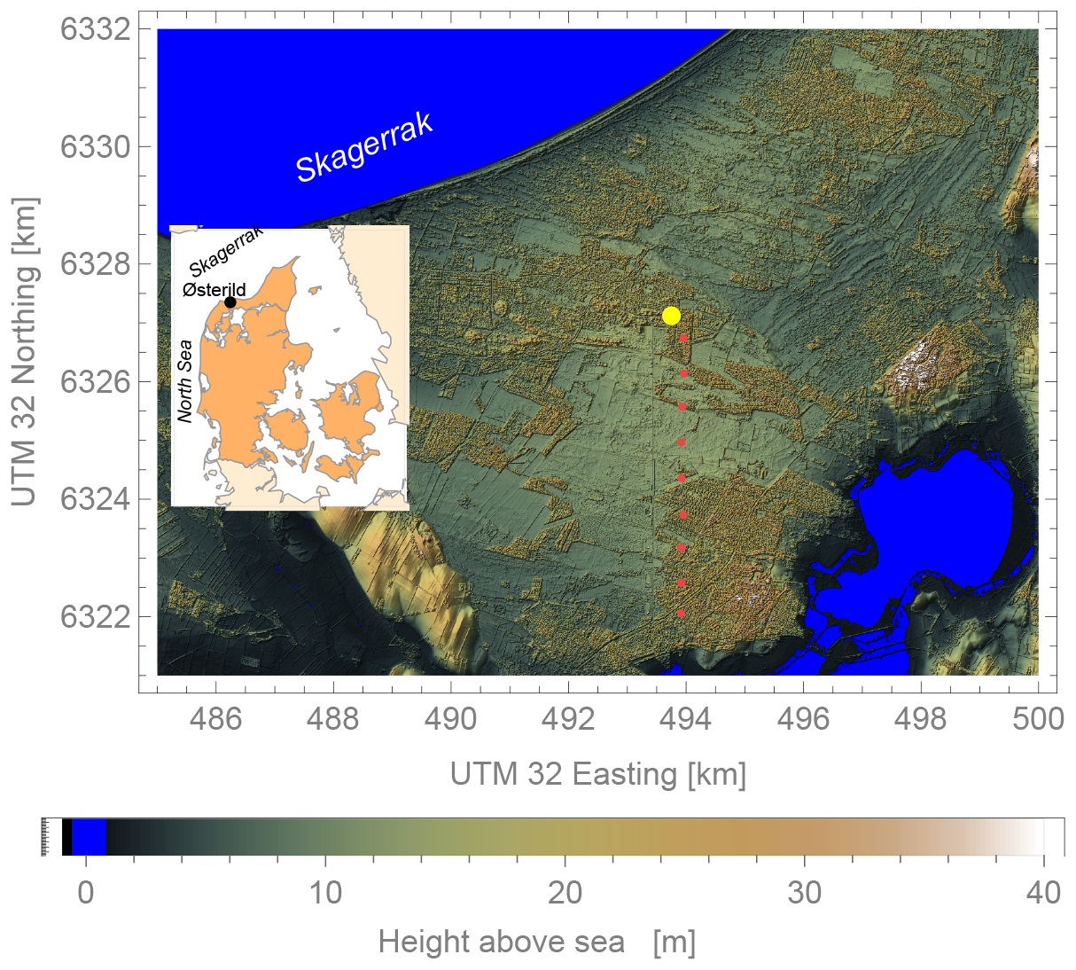
Figure 2 Position of the Østerild site in Denmark (inset) and a digital surface model of the surrounding area. The 250 m mast is in yellow, while the turbine stands at the test site around the red dots. It is seen that the area is relatively flat, and there is low forest to the northwest of the mast. The forest to the west of the turbine row has been cleared out to almost 2 km.

3.2 BEAM 6x lidar

The Halo Photonics by Lumibird BEAM 6x Wind Sciences pulsed lidar is used in this study because of its high-resolution of range gates along the beam. The lidar has six beams, of which five are inclined at an elevation angle of about 60° and arranged in a pentagonal pattern, i.e., with an azimuthal separation of 72°. The sixth beam is the vertical beam staring into zenith, directly measuring vertical velocities. A schematic of the lidar beams is displayed in Fig. 3. The lidar can measure radial velocities up to 1000 m, with the range gates separated by 3 m along the beam, which is an important quality of the instrument for the structure function estimation. The 3 m spacing should not be interpreted as the physical extent of the lidar beam's probe volume, which exceeds 20 m for the lidar understudy. Instead, the high range resolution achieved by HALO Photonics lidars results from their autocorrelation-based signal processing technique (Abdelazim et al., 2018), which allows overlapping Fourier windows to be applied to the accumulated autocorrelation matrix. The lidar was placed alongside the mast from 9 April to 6 December 2024. The lidar measures LOS velocities along a single beam in approximately 1 s, so one complete DBS scan takes ∼ 6 s. Following the manufacturer's recommendation, the signal-to-noise ratio (SNR) threshold of 1.015 is used to filter out the noisy Doppler measurements.

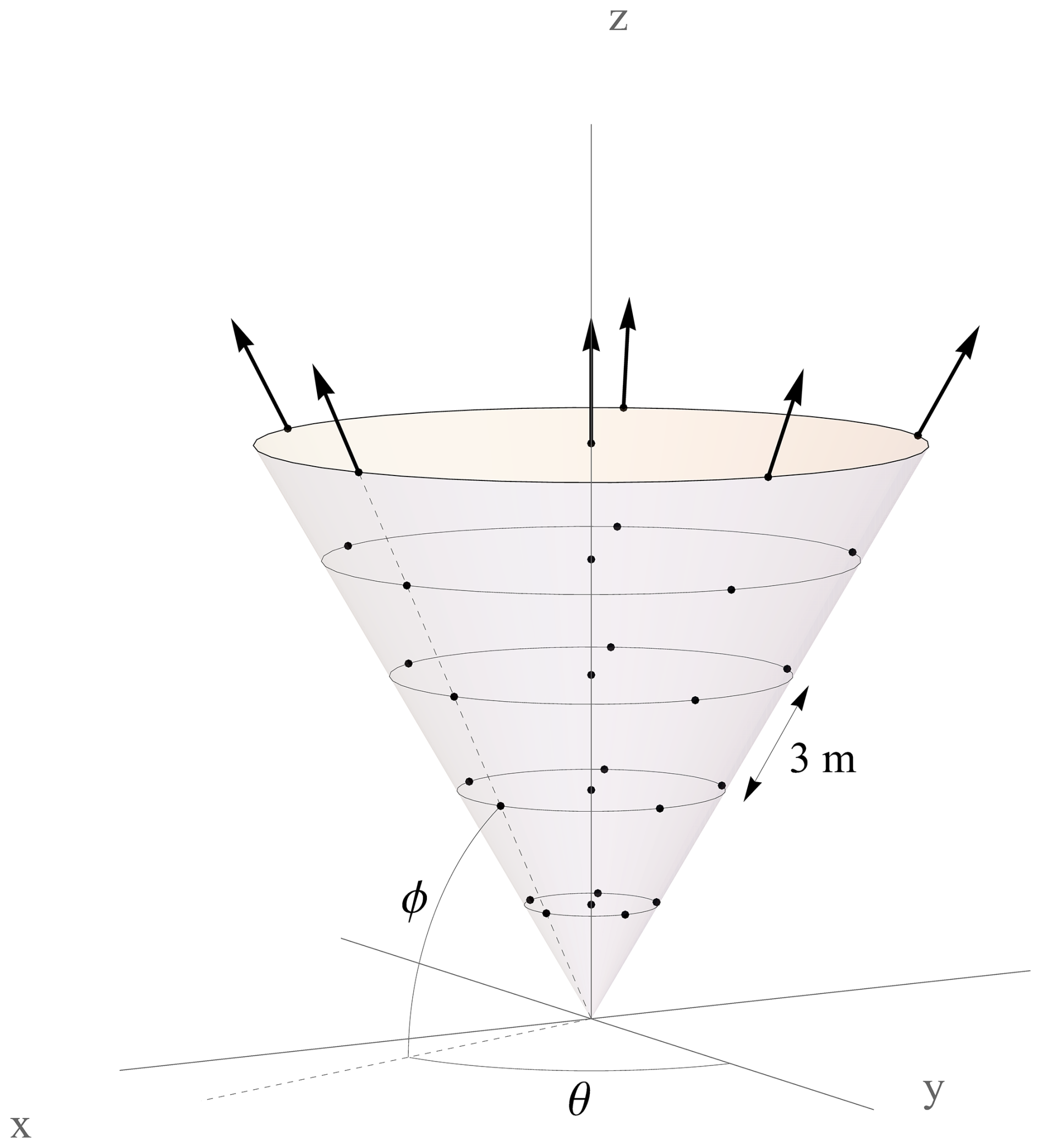
Figure 3 A schematic diagram showing the lidar beams' orientation and the distribution of range gates along the beams. The coordinate system used for the beams is also shown. Here θ represents the azimuth angle, and ϕ represents the elevation angle from the ground.

3.3 Ultrasonic anemometers

The mast has Metek USA-1 Scientific ultrasonic anemometers at elevations of 37, 103, 175, and 241 m. The anemometers are configured with a sampling frequency of 20 Hz. We convert the x, y, z speed components in the sonic output from a Cartesian coordinate system to the along-wind u, cross-wind v, and vertical w wind speed components. Afterward, we align the u component with the mean wind direction observed during each 10 min. Some peaks/outliers were observed in the sonic data and were removed using a Hampel filter (Liu et al., 2004) with a window size of 5 measurement points and an outlier threshold of 3 standard deviations. The ultrasonic anemometer data at 37 m is used to classify the data into different atmospheric stability classes by using the Obukhov length:

$$\begin{array}{}\text{(8)}& L_{\mathrm{o}}=-{\displaystyle \frac{u_{\ast }^{\mathrm{3}}}{\mathit{\kappa }(g/T)\stackrel{\mathrm{‾}}{w^{\prime }{\mathrm{\Theta }}_{\mathrm{v}}^{\prime }}}},\end{array}$$

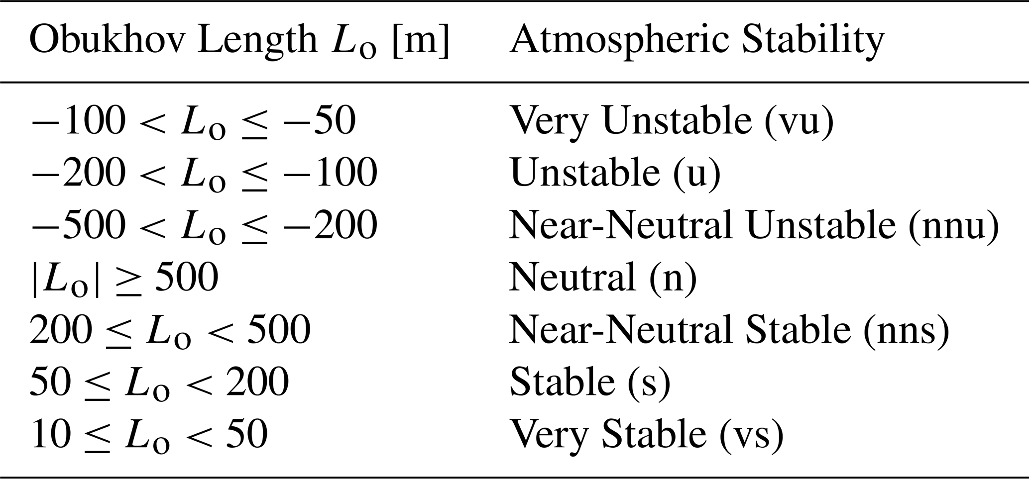
where u_∗ is the frictional velocity, κ is the von Kármán constant, g is the gravitational acceleration, T is the reference temperature, and $\stackrel{\mathrm{‾}}{w^{\prime }{\mathrm{\Theta }}_{\mathrm{v}}^{\prime }}$ is the virtual kinematic heat flux where Θ_v is the virtual potential temperature. Table 1 describes seven different stability classes from “Very Unstable” to “Very Stable” based on Obukhov length L_o.

Table 1 Stability classification based on the Obukhov length.

4 Workflow for estimating ε

In order to estimate the turbulent energy dissipation rate ε, the primary challenge is the detection of the inertial subrange. This can be done in several ways: either through the power spectral density of the wind components or by using the structure function method. For sonic anemometers, the straightforward way is to plot a wavenumber spectrum of the u, v, or w wind component by assuming Taylor's frozen turbulence hypothesis. In the inertial subrange, the one-point, two-sided velocity spectra in terms of wavenumber k₁ (where $k_{\mathrm{1}}=\mathrm{2}\mathit{\pi }f/\stackrel{\mathrm{‾}}{U}$; f is the frequency and $\stackrel{\mathrm{‾}}{U}$ is the mean wind speed) are given by:

$$\begin{array}{}\text{(9)}& F_u\left(k_{\mathrm{1}}\right)={\displaystyle \frac{\mathrm{9}}{\mathrm{55}}}\mathit{\alpha }{\mathit{\epsilon }}^{\mathrm{2}/\mathrm{3}}{k}_{\mathrm{1}}^{-\mathrm{5}/\mathrm{3}},\end{array}$$

for the along-wind spectrum and

$$\begin{array}{}\text{(10)}& F_v\left(k_{\mathrm{1}}\right)=F_w\left(k_{\mathrm{1}}\right)={\displaystyle \frac{\mathrm{12}}{\mathrm{55}}}\mathit{\alpha }{\mathit{\epsilon }}^{\mathrm{2}/\mathrm{3}}{k}_{\mathrm{1}}^{-\mathrm{5}/\mathrm{3}},\end{array}$$

for the cross-wind and vertical components, where α is the spectral Kolmogorov constant with a value of ∼ 1.52 (Pope, 2000). To detect the inertial subrange, a compensated spectrum $k_{\mathrm{1}}^{\mathrm{5}/\mathrm{3}}\cdot F_u\left(k_{\mathrm{1}}\right)$ is plotted against k₁. The region where $\mathrm{d}(k_{\mathrm{1}}^{\mathrm{5}/\mathrm{3}}\cdot F_u(k_{\mathrm{1}}\left)\right)/\mathrm{d}{k}_{\mathrm{1}}\approx \mathrm{0}$ represents the inertial subrange (Peña et al., 2019; Syed et al., 2023). Here, we only used wavenumber in the range $\mathrm{5}\times {\mathrm{10}}^{-\mathrm{2}}$ m⁻¹ < k₁ < 10⁰ m⁻¹ to detect the inertial subrange and allowed a slope deviation of only 10 %. This interval was selected after inspecting the spectra across the dataset's wind-speed range, where the inertial-subrange plateau was consistently observed within these wavenumber bounds. After detecting the range, ε_sonic is calculated using:

$$\begin{array}{}\text{(11)}& {\mathit{\epsilon }}_{\mathrm{sonic}}={\left[{\displaystyle \frac{\mathrm{55}}{\mathrm{9}\mathit{\alpha }}}\stackrel{\mathrm{‾}}{k_{\mathrm{1}}^{\mathrm{5}/\mathrm{3}}\cdot F_u\left(k_{\mathrm{1}}\right)}\right]}^{\mathrm{3}/\mathrm{2}},\end{array}$$

where $\stackrel{\mathrm{‾}}{\cdot }$ represents the mean value in the inertial subrange.

For the ε_lidar calculation from the BEAM 6x lidar, the structure function approach is adopted, meaning that we fit Eq. (6), where ε is the only unknown, to the measured lidar data. The benefit of such an approach is that since lidar beams measure LOS velocities at range gates physically separated by a distance at the same time, there is no need to assume Taylor's frozen turbulence hypothesis. The distance between the range gates is constant, i.e., 3 m. Furthermore, assuming that the sampling volume σ<ℒ_o, it would allow resolving the ε without ℒ_o dependence. The following steps are taken to derive ε_lidar from a single 10 min period from lidar LOS data:

1. For a selected height h, range gates within h ± 14 m are selected to get the measured longitudinal structure function from LOS velocities. For each beam, a mean structure function is computed from all scans over the 10 min period. Before the structure function is calculated, the mean line-of-sight velocity is subtracted at all heights. This is necessary to avoid an extra term in the structure function originating from the mean wind profile.

2. For the spatial+temporal averaging method, the mean wind vector was reconstructed using the LOS data from the five inclined beams to obtain U and θ_b for each 10 min period.

3. Another average from all six beams is taken to obtain the mean longitudinal structure function, D_meas. The lidar structure function model described in Eq. (6) is fitted to the inertial subrange of the mean measured structure function for r<28 m using the non-linear least squares fitting method to obtain ε_lidar. The following error function is minimized:

   $$\begin{array}{}\text{(12)}& \sum _{j=\mathrm{1}}^n{\left[{\log }_{\mathrm{10}}{D}_{\mathrm{lidar}}(r_j,\mathit{\epsilon },\mathit{\sigma })-{\log }_{\mathrm{10}}{D}_{\mathrm{meas}}\left(r_j\right)\right]}^{\mathrm{2}},\end{array}$$

   where n is the number of spatial separation distances included in the structure-function fit.

4. The lidar data is then classified into two different categories based on the percentage error obtained from the model fitting, defined as:

   $$\begin{array}{}\text{(13)}& \mathrm{\%}\mathrm{Error}=\left({\mathrm{10}}^{\mathrm{RMSE}}-\mathrm{1}\right)\times \mathrm{100},\end{array}$$

   where,

   $$\begin{array}{}\text{(14)}& \begin{array}{rl}& \mathrm{RMSE}=\\ & \sqrt{{\displaystyle \frac{{\sum }_{j=\mathrm{1}}^N{\left[{\log }_{\mathrm{10}}{D}_{\mathrm{lidar}}(r_j,\mathit{\epsilon },\mathit{\sigma })-{\log }_{\mathrm{10}}{D}_{\mathrm{meas}}\left(r_j\right)\right]}^{\mathrm{2}}}{n}}}.\end{array}\end{array}$$

   The first is the strict criterion, where only those 10 min periods are accepted where the %Error ≤ 15 %, whereas the relaxed criterion allows periods with the %Error ≤ 30 %.

As mentioned earlier, an appropriate value of σ is needed to account for the lidar's LOS filtering. Here we used a value of σ=9.4 m (Full Width at Half Maximum (FWHM) ≈ 22 m) for fitting the D_lidar model in Eq. (6) (only spatial averaging) and σ=7.9 m (FWHM ≈ 18.5 m) for the D_lidar model in Eq. (7) (spatial + temporal averaging). These values are based on the amount of bias or average systematic error obtained after fitting the modeled structure function using a range of σ values between 5 and 12 m with a step of 0.1 m. The selected σ values produced the least amount of bias in the ε estimation at all three heights (see Fig. 4) and therefore were used in the analysis presented hereafter.

Figure 4 Mean bias or systematic error produced by fitting the modeled structure function over a range of σ values for the D_lidar models presented in Eq. (6) (spatial) and Eq. (7) (spatial+temporal averaging), respectively.

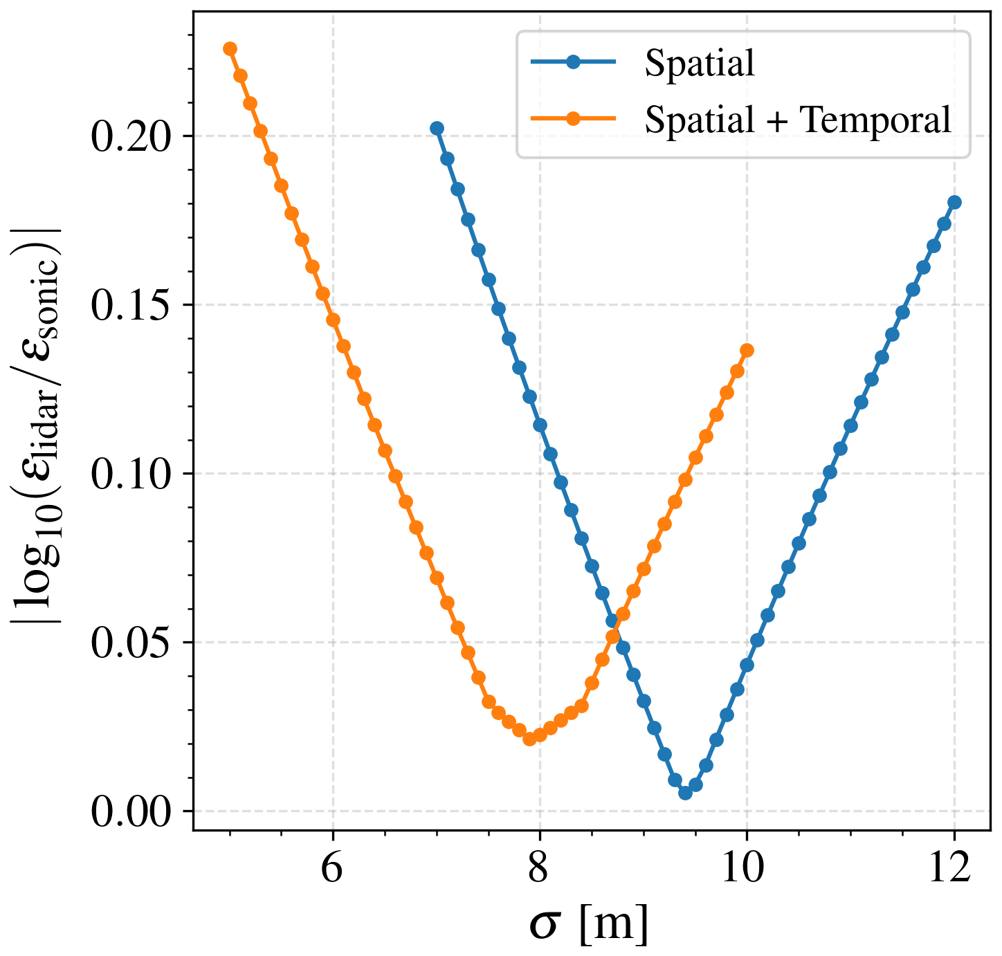
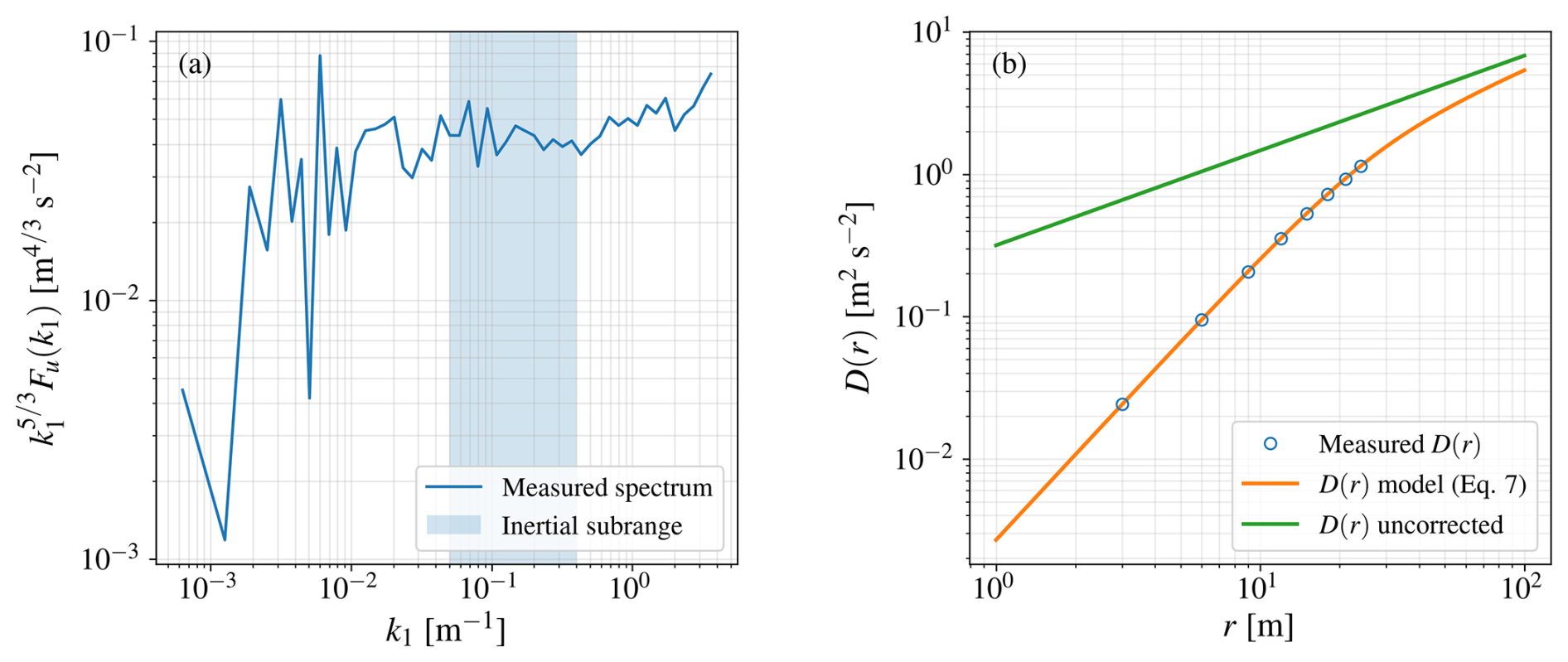
Figure 5 Two different ways used in this study to get turbulence energy dissipation rate ε. (a) Sonic anemometer: an illustration of the compensated spectrum $k_{\mathrm{1}}^{\mathrm{5}/\mathrm{3}}\cdot F_u\left(k_{\mathrm{1}}\right)$ and the inertial subrange at 103 m above ground level. (b) BEAM 6x lidar: an example of the measured structure function (blue markers) and the D_lidar model in Eq. (7) fitted over it (orange line). The unfiltered D(r) with Kolmogorov's scaling of $r^{\mathrm{2}/\mathrm{3}}$ is also shown (green line).

An illustration of estimating ε from sonic and lidar data is shown in Fig. 5. For both sonic anemometers and lidar, ε is calculated for those 10 min time periods where $\stackrel{\mathrm{‾}}{U}$ ≥ 4 m s⁻¹ and the wind direction ∈ [0–120°] or [225–360°]. The winds coming from the south sector [121–224°] were discarded to avoid wake flow from wind turbines at the test site and the wake from the mast itself. This study includes ε results from three heights: 103, 175, and 241 m. Results at a height of 37 m are excluded from the analysis because the pulsed lidar is blind below 30 m, and there are not enough data points to obtain a realistic second-order structure function.

The agreement between the lidar- and sonic-derived dissipation rates is evaluated in log space because ε spans several orders of magnitude. Two different metrics are used to judge the quality of comparison. The first one is the Pearson correlation coefficient (ρ) calculated between log ₁₀(ε_lidar) and log ₁₀(ε_sonic). This metric represents the scatter between the lidar and sonic measurements, i.e., the strength of their linear association. To judge whether the sonic and lidar-obtained ε values vary at the same rate and if there is a systematic offset, a second metric is used: an ordinary least-squares (OLS) regression. For the OLS regression, ${\log }_{\mathrm{10}}\left({\mathit{\epsilon }}_{\mathrm{lidar}}\right)=a{\log }_{\mathrm{10}}\left({\mathit{\epsilon }}_{\mathrm{sonic}}\right)+b$, where a and b represent the slope and intercept of the OLS regression line.

5 Results

The atmospheric conditions observed at the Østerild test site during the lidar measurement period were predominantly neutral, with about 55 % of the data falling into one of three categories: nns, n, or nnu. Stable atmospheric conditions (s, vs) occurred about 30 % of the measurement time, while the unstable conditions (u, vu) were present for about only 15 % of the time. With this in mind, let's view the D_lidar(r) model fitting error, described in Eq. (13), as a function of the atmospheric stability in Fig. 6 at the three measurement heights of 103, 175, and 241 m. The neutral conditions (nns, n, nnu) produced the lowest fitting errors at all three heights. The unstable conditions (u and vu) showed slightly higher errors when fitting the structure function model over the measured data. The highest model-fitting errors were observed under very stable (vs) atmospheric conditions, as these conditions have the least atmospheric turbulence, making it difficult to identify the inertial subrange. We also observed an increase in fitting errors with height, with the median and maximum error values highest at 241 m across all stability conditions. This is caused by a combination of a weaker lidar return signal with increasing height and weaker turbulence fluctuations. The resulting lower signal-to-noise ratio makes it harder to detect the inertial subrange and fitting of ε.

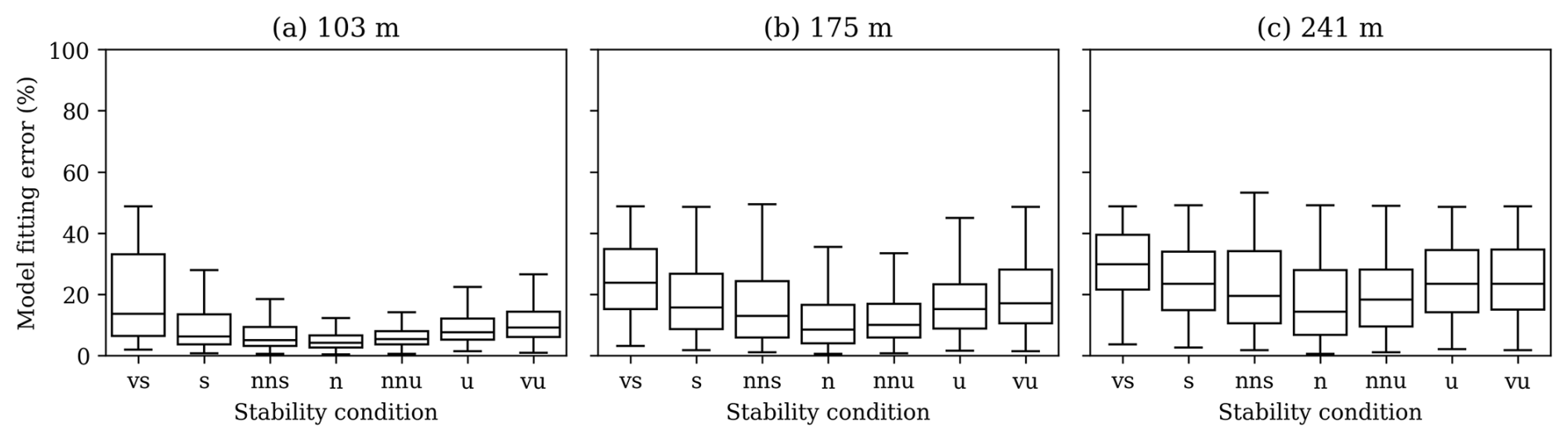
Figure 6 The model fitting error as a function of the seven stability classes described in Table 1 at three different heights: (a) 103 m, (b) 175 m, and (c) 241 m. The box plot shows the median (center line) and the first and third quartiles. The whiskers represent the minimum and maximum values of the observed error.

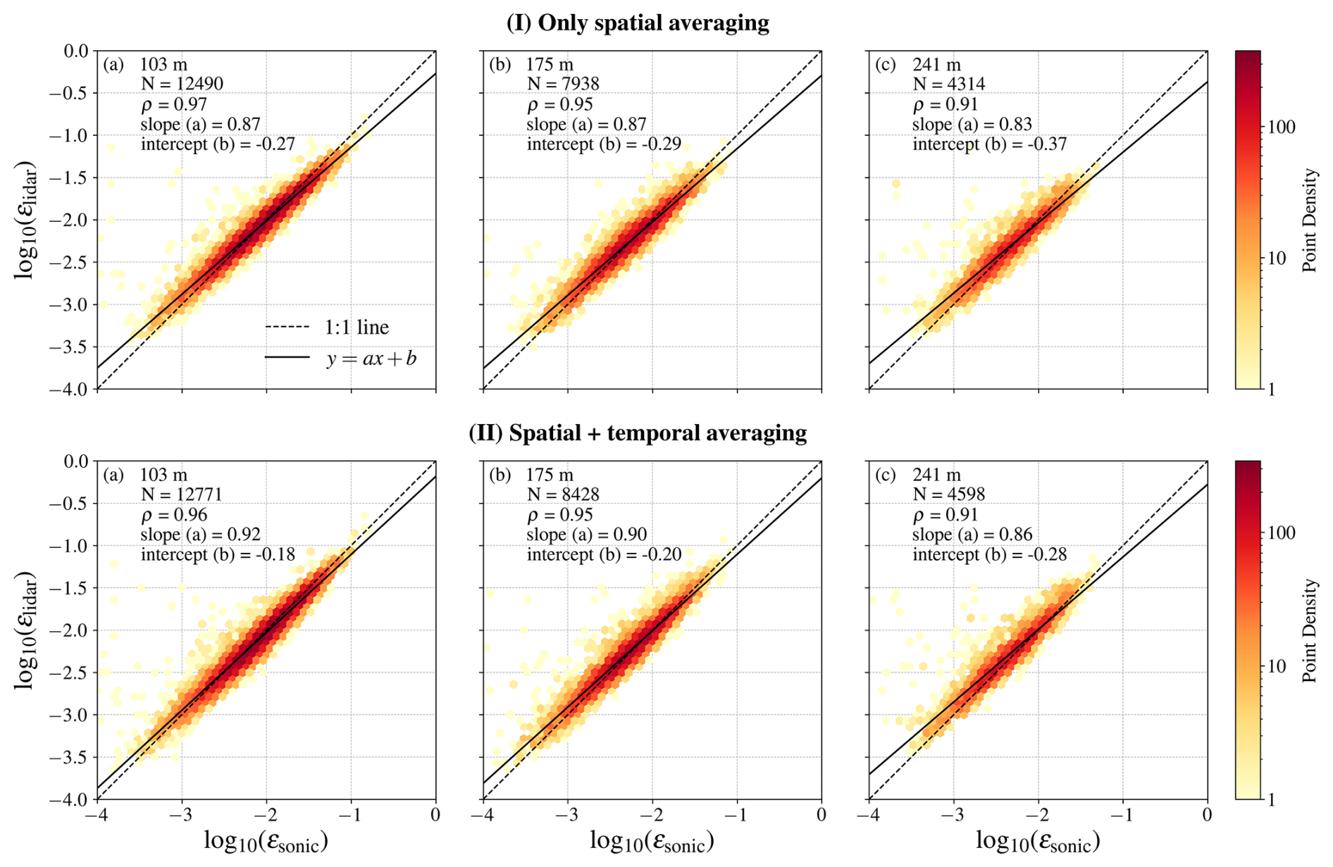
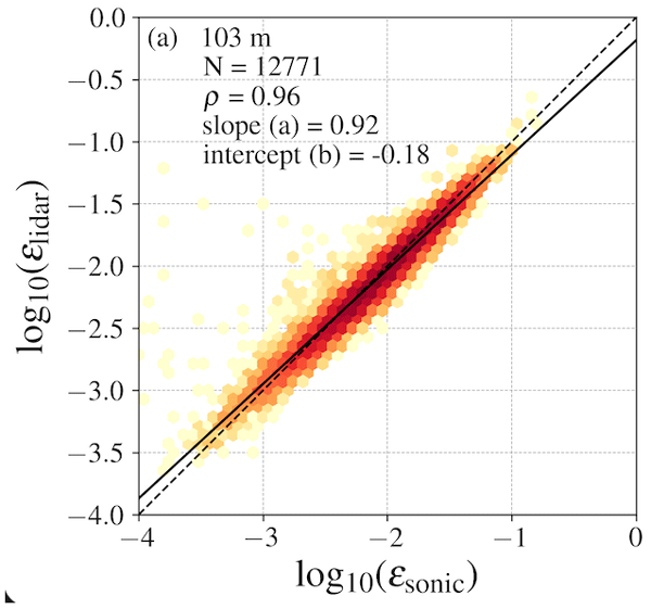
Figure 7 Comparison of ε_lidar with ε_sonic at three heights of (a) 103 m, (b) 175 m, and (c) 241 m for the strict criterion (model fitting error ≤ 15 %). The top panel shows (I) only spatial averaging, where Eq. (6) is fitted over lidar LOS structure function measurements. The bottom panel displays (II) Spatial + temporal averaging using Eq. (7). The values are plotted on a log-log plot, and the black dashed line represents 1 : 1 correspondence. OLS regression line ${\log }_{\mathrm{10}}\left({\mathit{\epsilon }}_{\mathrm{lidar}}\right)=a{\log }_{\mathrm{10}}\left({\mathit{\epsilon }}_{\mathrm{sonic}}\right)+b$ is also plotted in blue color. The number of 10 min samples used in the plots (N) and the Pearson correlation coefficient (ρ) are also mentioned. The point density represents the number of data points in each hexagonal cell.

Figure 8 Same as Fig. 7 but for the relaxed error criterion (model fitting error ≤ 30 %).

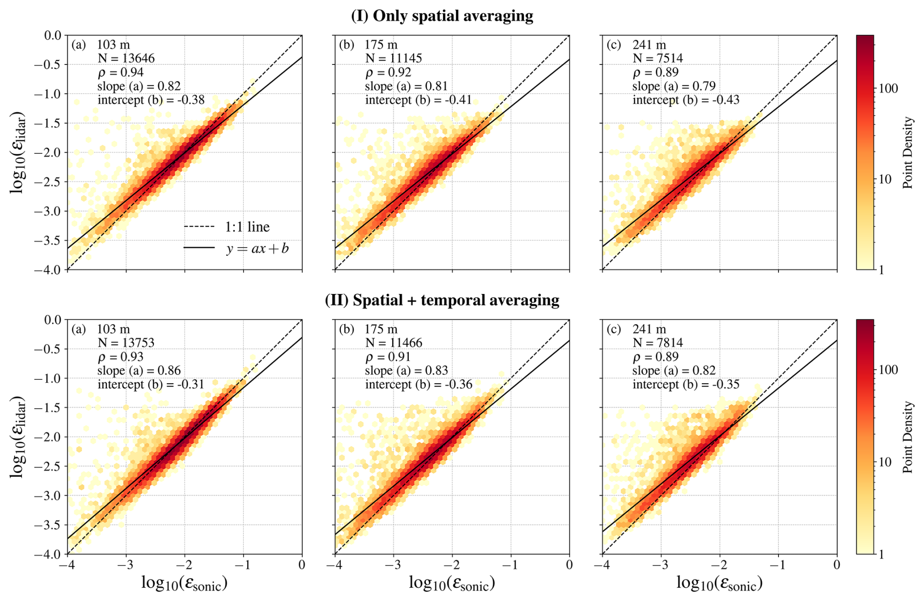
The comparison of turbulence energy dissipation rates obtained from lidar and sonic anemometers at the three heights of 103, 175, and 241 m is displayed in Figs. 7 and 8 for the strict and relaxed error criteria, respectively. The data shown here represent all seven stability classes and are therefore not subdivided. Each figure is further divided into two panels: (I) only spatial averaging, where the ε_lidar values are obtained by fitting Eq. (6) over the measured structure function data, and (II) spatial + temporal averaging, where Eq. (7) is fitted over the data. In both panels, the number of available 10 min time periods (N) that qualify for all the requirements, i.e., wind speed, wind direction, and whether the fitting error is within the defined limit, is highest at 103 m. The sample number subsequently decreases at higher heights due to increased model-fitting error and greater difficulty in detecting the inertial subrange.

In Fig. 7, the scatter between the data points at all heights is minimal for both panels which can be observed by nearly identical values of ρ, i.e., 0.96–0.97 at 106 m, 0.95 at 175 m, and 0.91 at 241 m. These large values of ρ imply a strong linear association between the model-predicted ε_lidar and measured ε_sonic values. However, ρ alone does not describe the full picture. Looking at the OLS regression lines for both the spatial-averaging and spatial + temporal-averaging panels, one can clearly see the utility of including temporal averaging in the fitting process. The slope of the OLS regression line (a) represents the rate of change of ε_lidar with ε_sonic while the intercept (b) reveals any offset. Including temporal averaging in the fitting process significantly improves predictions of ε_lidar values: a 5-percentage-point increase in a at 103 m and a 3-point increase at 175 m and 241 m. Similarly, the intercept b approaches zero with temporal averaging. The results show that the model without temporal averaging (in Eq. 6) tends to overestimate ε_lidar when turbulence is low and to underestimate it under strong turbulence.

In Fig. 8, similar trends are observed for the relaxed criterion (≤ 30 % model fitting error). For the relaxed criterion, however, the number of available 10 min periods are increased significantly: from 90 % of the available data to almost 100 % at 103 m, from 60 % of the available data to 85 % at 175 m, and from 40 % of the available data to 70 % at 241 m. This increase is marked by a very slight decrease in ρ values: 0.93–0.94 at 103 m, 0.91–0.92 at 175 m, and 0.89 at 241 m. This implies that relaxing the error criterion significantly increases the amount of available data without severely sacrificing the strong linear association between lidar and sonic ε. Although the number of 10 min periods where lidar overestimates ε increases, they are still relatively smaller in number, as indicated by the color in the density plots (see Fig. 8). The OLS regression parameters a and b also improve under the relaxed fitting criterion when temporal averaging effects are included. 4 percentage points increase in a at 103 m, 2 points increase at 175 m, and 3 points increase at 241 m. The intercept value also moves closer to zero in the plots with spatial + temporal averaging. These results highlight the importance of including both kinds of probe volume-averaging effects, i.e., spatial and temporal, when calculating the second-order structure functions. Further plots will show only the results from fitting the spatial + temporal model (Eq. 7) to the data.

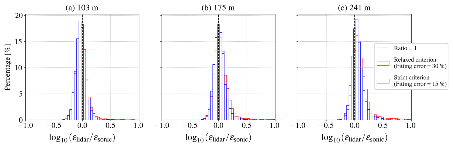
Figure 9 Histogram of ${\log }_{\mathrm{10}}({\mathit{\epsilon }}_{\mathrm{lidar}}/{\mathit{\epsilon }}_{\mathrm{sonic}})$ at the three heights under investigation, i.e, (a) 103 m, (b) 175 m, and (c) 241 m. Histograms are presented for both relaxed fitting criterion (in red color) and strict fitting criterion (in blue color).

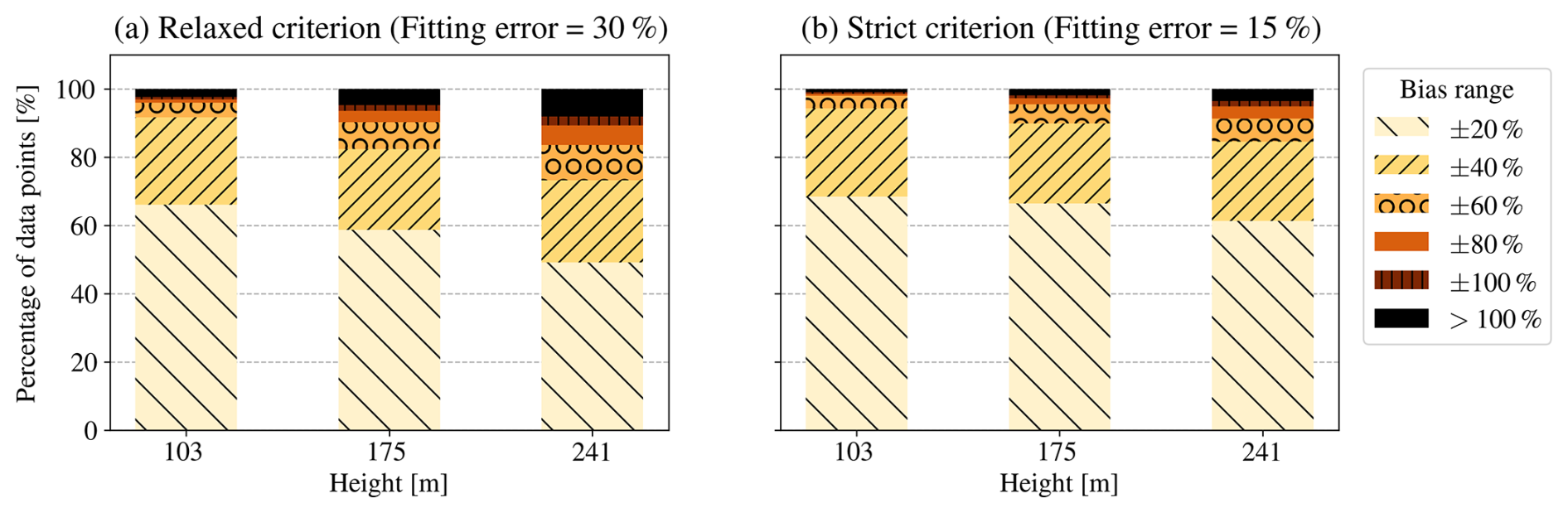
Figure 10 Bias ranges of ε_lidar relative to ε_sonic. More than 60 % of the lidar-derived turbulence energy dissipation rate values lie within ±20 % of those derived from sonic anemometers.

The bias analysis of the lidar-derived turbulence energy dissipation rates is presented in Figs. 9 and 10. Histograms of the ${\log }_{\mathrm{10}}({\mathit{\epsilon }}_{\mathrm{lidar}}/{\mathit{\epsilon }}_{\mathrm{sonic}})$ are illustrated in Fig. 9 for the three heights while the bias ranges of ε_lidar relative to ε_sonic are shown in Fig. 10. These plots are shown for both relaxed and strict error criteria. From the histogram plots, one can see that most of the data is centered at ${\log }_{\mathrm{10}}({\mathit{\epsilon }}_{\mathrm{lidar}}/{\mathit{\epsilon }}_{\mathrm{sonic}})=\mathrm{0}$. For the strict criterion, there is no tail in the distribution on either side of the center. But for the relaxed criterion, a small tail on the right side, i.e. ${\log }_{\mathrm{10}}({\mathit{\epsilon }}_{\mathrm{lidar}}/{\mathit{\epsilon }}_{\mathrm{sonic}})>\mathrm{0}$ is observed, which shows those 10 min periods where the lidar overestimates ε. Combined, these data points represent less than 5 % of the total data analyzed.

Another interesting way to look at the bias is to categorize the data in bias ranges, as seen in Fig. 10. For all three heights, more than 50 % of the lidar obtained ε_lidar values are within ±20 % range of the ε_sonic. Similarly, > 90 % and > 75 % of ε_lidar values obtained are inside the ±40 % range of the ε_sonic for the strict and relaxed error criteria, respectively. These results clearly show the high accuracy of the structure function method in determining the turbulence energy dissipation rate from a lidar with a small range-gate spacing.

6 Discussion

The utility of the modeled structure function containing the lidar filtering effect in estimating ε is clearly observed in the above shown comparison. The largest source of random error in this method arises from the detection of the inertial subrange. It was challenging to detect an inertial subrange during very stable atmospheric conditions and during low wind speeds (< 5 m s⁻¹) due to the lidar's filtering of small-scale turbulence structures. Since we used only the high-level lidar data, i.e., LOS velocities, to estimate ε, any fluctuations smaller than the lidar probe volume length are filtered out. One way to overcome this is to use low-level lidar data, e.g., Doppler spectrum width, or to minimize the range gate spacing of the lidar beams. A comparison between the DSW and the structure function methods is not performed here but is left for future investigation.

The choice of the Kolmogorov constant C_K also impacts the estimated ε values. C_K is reported to be 2.1 ± 0.1 in the literature (Pope, 2000). For the fixed measured structure function, the turbulence energy dissipation rate scales as $\mathit{\epsilon }\propto C_{\mathrm{K}}^{-\mathrm{3}/\mathrm{2}}$, thus using C_K=2.1 instead of C_K=2 would lower the ε estimates by approximately 7 %. This is true for the absolute comparison between ε estimates obtained from a single instrument/method. However, in the relative comparison between ε values obtained from lidar and sonic anemometer, the choice of C_K does not matter. The sonic-based dissipation rates are inferred using the spectral Kolmogorov constant α=1.52, which comes from C_K=2 (a value of C_K=2.1 results in α=1.6). Therefore, although the choice of C_K does introduce uncertainty in the absolute magnitude of the obtained ε values, it does not affect the relative lidar-sonic comparison. It should be noted that two different methods are used to estimate ε from sonic anemometer and lidar measurements: the spectral and structure function methods, respectively. However, both estimates are based on the same fundamental assumptions of local isotropy in the inertial subrange and Kolmogorov scaling. Some slight systematic differences may arise between the two methods owing to differences in the fitting procedure and measurement filtering.

Unlike in older systems, instrument noise in modern lidar systems, such as the one used in this study, can be neglected (Mann et al., 2009; Sathe and Mann, 2013). Since the magnitude of ε spans the order of multiple decades (10⁻⁴ to 10⁻¹), the instrument noise can possibly pollute the measurements, especially at low ε values. However, the random errors from the instrument noise are reduced by using a conservative SNR threshold. A lower threshold would allow more data points at the cost of increasing the random error. Furthermore, the statistical uncertainty associated with the lidar-measured ε is reduced by taking the mean structure function across all six beams over the 10 min period and then fitting the model to that averaged measured structure function.

The method presented in this article is not specific to the BEAM 6x lidar. In principle, it could be applied to any other pulsed Doppler lidar if the range-gate spacing is sufficiently smaller over the region of interest. The advantage of the BEAM 6x configuration here is that 3 m range gate spacing is available throughout the atmospheric column, allowing the method to be applicable over an extended range. The excellent correlation between ε obtained from the lidar and sonic anemometer indicates that ε can be computed directly from the inertial subrange, provided that σ<ℒ_o. This also requires that the inertial subrange is detected with a high certainty, where the high range-gate resolution of the Beam 6x lidar proves especially useful. Large model fitting errors observed in the very stable atmospheric conditions (see Fig. 6) may indicate that the inertial subrange may not be detected properly or that the turbulence length scales are relatively small, i.e., ℒ_o<σ. A simple possible solution would be to include a correction parameter for very stable conditions in the structure function model, or to use a lidar with even smaller range-gate spacing. Recently introduced Halo Photonics by Lumibird BEAM 6x Wind Power lidar with a range gate resolution of 1.5 m along the beam can be used to resolve small-scale turbulence even further, but has not been tested yet. For wind energy applications, turbulence intensity (TI) is a more practical parameter to describe turbulence instead of ε. An ongoing study aims to accurately estimate the TI parameter using the methods described in this paper. The aim is to correct the LOS variance estimates for each beam once we know ε, and then use LOS variances to compute the Reynolds stress tensor using a method described by Eberhard et al. (1989) and Sathe et al. (2015).

7 Conclusions

A second-order longitudinal structure function model for lidar LOS velocities is presented in this article. The model also includes a Gaussian filter to account for probe volume (both spatial and temporal averaging effects) within a pulsed lidar beam. The model is used to measure ε at three heights: 103, 175, and 241 m, using a six-beam pulsed lidar. The lidar-obtained ε values were compared with those from ultrasonic anemometers.

The second-order structure function model presented here can be used to estimate ε using a standalone lidar with high range-gate resolution (i.e., small spacing between range gates). The lidar used here has a range-gate spacing of 3 m and can effectively detect the inertial subrange. We compared almost 8 months of lidar-measured ε with the corresponding sonic-measured ε and found an excellent correlation between the two datasets. We observed Pearson correlation coefficient (ρ) values of more than 0.9 across all three heights, significantly higher than in similar previous studies and methods (Smalikho and Banakh, 2017; Wildmann et al., 2020; Bodini et al., 2018). The observed bias was also very small, i.e., more than 50 % of all the lidar-measured ε values lie within ±20 % of the sonic-measured values.

It was observed that the main source of random errors in lidar-measured ε values is the improper detection of the inertial subrange. Since the structure function method relies heavily on detecting the inertial subrange, relaxing the error criterion during model fitting can significantly increase random errors in the estimated ε. It is therefore advisable to be cautious when using this method under low wind-speed conditions (< 5 m s⁻¹), where reduced atmospheric turbulence may lead to contamination by instrument noise. Under very stable atmospheric conditions, detecting the inertial subrange becomes even more challenging due to smaller turbulence length scales, which are filtered out by the lidar's probe volume-averaging process. Prospective studies may include quantifying the random error arising from instrumental noise and comparing it with that of other similar methods, such as the Doppler spectrum width method, to estimate ε. Additionally, the effect of lidar motion on ε measurements in a floating configuration, which we expect to be null, would also be an interesting investigation.

Appendix A: Derivation of lidar longitudinal structure function

It is convenient to transform the square of the integral in Eq. (5) to a double integral such that the ensemble average can be moved inside the integrals:

$$\begin{array}{}\text{(A1)}& \begin{array}{rl}{D}_{\mathrm{lidar}}\left(r\right)=& \underset{-\mathrm{\infty }}{\overset{\mathrm{\infty }}{\iint }}〈\left\{v(x+s_{\mathrm{1}})-v(x+r+s_{\mathrm{1}})\right\}\\ & \times \left\{v(x+s_{\mathrm{2}})-v(x+r+s_{\mathrm{2}})\right\}〉\\ & \times \mathit{\phi }\left(s_{\mathrm{1}}\right)\mathit{\phi }\left(s_{\mathrm{2}}\right)\mathrm{d}{s}_{\mathrm{1}}\mathrm{d}{s}_{\mathrm{2}}.\end{array}\end{array}$$

Expanding the parentheses and using the definition of the covariance function $R\left(r\right)\equiv \langle v\left(x\right)v(x+r)\rangle$, the product of the curly parentheses can be written as

$$\begin{array}{}\text{(A2)}& \mathrm{2}R(s_{\mathrm{1}}-s_{\mathrm{2}})-R(s_{\mathrm{1}}-s_{\mathrm{2}}-r)-R(s_{\mathrm{1}}-s_{\mathrm{2}}+r),\end{array}$$

and if we further exploit the fact that due to the symmetry of φ the integrals over the last two terms are the same, and the formal relation $D\left(r\right)=\mathrm{2}\left(R\right(\mathrm{0})-R(r\left)\right)$, the term can be written as

$$\begin{array}{}\text{(A3)}& D(s_{\mathrm{1}}-s_{\mathrm{2}}-r)-D(s_{\mathrm{1}}-s_{\mathrm{2}}).\end{array}$$

We now transform the integration variables into $s=s_{\mathrm{1}}-s_{\mathrm{2}}$ and $s^{\prime }=s_{\mathrm{1}}+s_{\mathrm{2}}$ with the Jacobian determinant $|\partial (s{s}^{\prime })/\partial (s_{\mathrm{1}}{s}_{\mathrm{2}}\left)\right|=\mathrm{2}$ such that

$$\begin{array}{}\text{(A4)}& \begin{array}{rl}{D}_{\mathrm{lidar}}\left(r\right)=& \underset{-\mathrm{\infty }}{\overset{\mathrm{\infty }}{\int }}\left\{D(s-r)-D\left(s\right)\right\}\\ & \times \underset{-\mathrm{\infty }}{\overset{\mathrm{\infty }}{\int }}{\displaystyle \frac{\mathrm{1}}{\mathrm{2}}}\mathit{\phi }\left({\displaystyle \frac{s+s^{\prime }}{\mathrm{2}}}\right)\mathit{\phi }\left({\displaystyle \frac{s^{\prime }-s}{\mathrm{2}}}\right)\mathrm{d}{s}^{\prime }\mathrm{d}s.\end{array}\end{array}$$

The inner integral over s^′ is essentially a convolution of two Gaussian functions, so the expression becomes

$$\begin{array}{}\text{(A5)}& \begin{array}{rl}{D}_{\mathrm{lidar}}\left(r\right)=& \underset{-\mathrm{\infty }}{\overset{\mathrm{\infty }}{\int }}\left\{D(s-r)-D\left(s\right)\right\}\\ & \times {\displaystyle \frac{\mathrm{1}}{\mathrm{2}\sqrt{\mathit{\pi }}\mathit{\sigma }}}\exp \left(-{\displaystyle \frac{s^{\mathrm{2}}}{\mathrm{4}{\mathit{\sigma }}^{\mathrm{2}}}}\right)\mathrm{d}s.\end{array}\end{array}$$

Using the inertial subrange expression of the structure function Eq. (2) and consulting the symbolic algebra capabilities of Mathematica, we finally arrive at Eq. (6).

Additional temporal averaging

In the discussion so far, we have ignored the temporal averaging in Eq. (3). In reality, this equation should read

$$\begin{array}{}\text{(A6)}& v_r\left(\mathit{x}\right)={\displaystyle \frac{\mathrm{1}}{\mathrm{\Delta }t}}\underset{-\mathrm{\Delta }t/\mathrm{2}}{\overset{\mathrm{\Delta }t/\mathrm{2}}{\int }}\underset{-\mathrm{\infty }}{\overset{\mathrm{\infty }}{\int }}\mathit{\phi }\left(s\right)\mathit{n}\cdot \mathit{v}(s\mathit{n}+\mathit{x}+tU{\mathit{e}}_{\mathrm{1}})\mathrm{d}s\mathrm{d}t,\end{array}$$

where U is the mean wind speed, Δt the time over which the lidar's Doppler signal is averaged, typically between 0.2 and 2 s, and e₁ is a unit vector in the mean wind direction. We have implicitly used Taylor's hypothesis in this equation. The statistics of this expression of the velocity does not only depend on the length scale σ in the weighting function φ, which is the case when the turbulence on scales smaller than σ is isotropic, but also on the time averaging Δt and the angle between n and e₁.

Let us first look at the simplest case where n∥e₁, that is, the lidar beam is aligned with the mean wind. In this case Eq. (A6) is, using $\mathit{n}\cdot \mathit{v}=v_{\mathrm{1}}$,

$$\begin{array}{}\text{(A7)}& v_r\left(\mathit{x}\right)={\displaystyle \frac{\mathrm{1}}{\mathrm{\Delta }t}}\underset{-\mathrm{\Delta }t/\mathrm{2}}{\overset{\mathrm{\Delta }t/\mathrm{2}}{\int }}\underset{-\mathrm{\infty }}{\overset{\mathrm{\infty }}{\int }}\mathit{\phi }\left(s\right)v_{\mathrm{1}}\left((s+tU){\mathit{e}}_{\mathrm{1}}+\mathit{x}\right)\mathrm{d}s\mathrm{d}t,\end{array}$$

or, substituting $s^{\prime }=s+tU$,

$$\begin{array}{}\text{(A8)}& v_r\left(\mathit{x}\right)=\underset{-\mathrm{\infty }}{\overset{\mathrm{\infty }}{\int }}\stackrel{\mathrm{̃}}{\mathit{\phi }}\left(s^{\prime }\right)v_{\mathrm{1}}(s^{\prime }{\mathit{e}}_{\mathrm{1}}+\mathit{x})\mathrm{d}{s}^{\prime },\end{array}$$

where

$$\begin{array}{}\text{(A9)}& \stackrel{\mathrm{̃}}{\mathit{\phi }}\left(s^{\prime }\right)={\displaystyle \frac{\mathrm{1}}{\mathrm{\Delta }t}}\underset{-\mathrm{\Delta }t/\mathrm{2}}{\overset{\mathrm{\Delta }t/\mathrm{2}}{\int }}\mathit{\phi }(s^{\prime }-tU)\mathrm{d}t.\end{array}$$

So, the velocity field v₁ is folded with $\stackrel{\mathrm{̃}}{\mathit{\phi }}$ whose transfer function or absolute squared Fourier transform is

$$\begin{array}{}\text{(A10)}& {\left|\widehat{\stackrel{\mathrm{̃}}{\mathit{\phi }}}\left(k\right)\right|}^{\mathrm{2}}={\mathrm{e}}^{-k^{\mathrm{2}}{\mathit{\sigma }}^{\mathrm{2}}}{\mathrm{sinc}}^{\mathrm{2}}\left({\displaystyle \frac{\mathrm{\Delta }tUk}{\mathrm{2}}}\right).\end{array}$$

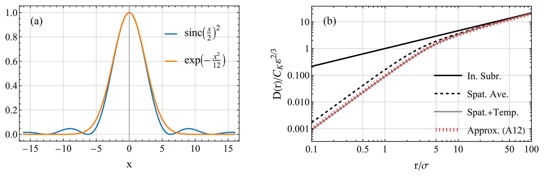
Figure A1 (a) Comparison of the sinc-term in Eq. (A10) with its Gaussian approximation in Eq. (A11). (b) Comparison of structure functions: Inertial subrange (solid black), spatial averaging only with the lidar's spatial weighting function Eq. (6) (dashed), also including temporal averaging with $\mathrm{\Delta }tU/\mathit{\sigma }=\mathrm{4}$ (gray), and the approximation using Eqs. (A12) and (6) (red, dashed).

By matching the second derivative of this function with a single Gaussian, we arrive at

$$\begin{array}{}\text{(A11)}& {\left|\widehat{\stackrel{\mathrm{̃}}{\mathit{\phi }}}\left(k\right)\right|}^{\mathrm{2}}\approx {\mathrm{e}}^{-k^{\mathrm{2}}{\mathit{\sigma }}^{\mathrm{2}}}{\mathrm{e}}^{-\frac{(\mathrm{\Delta }tUk{)}^{\mathrm{2}}}{\mathrm{12}}}\end{array}$$

such that we can approximate the process of spatial and temporal averaging with a single spatial averaging using the width parameter $\stackrel{\mathrm{̃}}{\mathit{\sigma }}$, defined by

$$\begin{array}{}\text{(A12)}& \textcolor{red}{}\end{array}$$

reusing the expression Eq. (6). A comparison of the sinc-function in Eq. (A10) and its approximation in Eq. (A11) is shown in Fig. A1a. In this figure (right), we also show the calculated inertial subrange structure functions with various kinds of averaging. In this example, we choose a strong spatial averaging (high wind speed) with $\mathrm{\Delta }tU/\mathit{\sigma }=\mathrm{4}$, meaning that if σ≈9 m and Δt=1 s, then U would have to be 36 m s⁻¹. The spatial plus temporal averaging is calculated numerically using Eq. (A4), but with $\stackrel{\mathrm{̃}}{\mathit{\phi }}$ from Eq. (A9) instead of φ. All curves match when r≫σ but for small r, ignoring the temporal averaging overestimates the structure function with 80 %, while the approximation Eq. (A12) using Eq. (6) only overestimates with 4 %. The wind speeds analyzed here are generally much smaller than 36 m s⁻¹, and the corresponding errors are quadratically smaller, so we conclude Eq. (A12) is a very good approximation.

The question now arises whether Eq. (A12) is a good approximation, even in the case where $\mathit{n}\cancel{\Vert }{\mathit{e}}_{\mathrm{1}}$, i.e. the beam is not aligned with the wind direction. With $R_r\left(\mathit{x}\right)=\langle v_r\left({\mathit{x}}^{\prime }\right)v_r({\mathit{x}}^{\prime }+\mathit{x})\rangle$ the lidar-measured structure function can be written as

$$\begin{array}{}\text{(A13)}& D_{\mathrm{lidar}}\left(r\right)=\mathrm{2}\left(〈v_r^{\mathrm{2}}〉-R_r\left(r\mathit{n}\right)\right).\end{array}$$

We can express both terms in the above equation in terms of the three-dimensional spectrum of v_r, which can be calculated in the following way. The Fourier transform of v_r is

$$\begin{array}{}\text{(A14)}& {\widehat{v}}_r\left(\mathit{k}\right)=\widehat{\mathit{\phi }}(\mathit{k}\cdot \mathit{n})\mathrm{sinc}\left({\displaystyle \frac{\mathrm{\Delta }tU{k}_{\mathrm{1}}}{\mathrm{2}}}\right)\mathit{n}\cdot \widehat{\mathit{v}}\left(\mathit{k}\right),\end{array}$$

and the spectrum is the mean of the absolute square of ${\widehat{v}}_r$:

$$\begin{array}{}\text{(A15)}& {\mathrm{\Phi }}_r\left(\mathit{k}\right)={\mathrm{e}}^{-(\mathit{k}\cdot \mathit{n}{)}^{\mathrm{2}}{\mathit{\sigma }}^{\mathrm{2}}}{\mathrm{sinc}}^{\mathrm{2}}\left({\displaystyle \frac{\mathrm{\Delta }tU{k}_{\mathrm{1}}}{\mathrm{2}}}\right)n_i{n}_j{\mathrm{\Phi }}_{ij}\left(\mathit{k}\right),\end{array}$$

where Φ_ij the spectral tensor of the velocity field.

Since

$$\begin{array}{}\text{(A16)}& R_r\left(r\mathit{n}\right)=\int {\mathrm{\Phi }}_r\left(\mathit{k}\right)\exp (-\mathrm{i}r\mathit{k}\cdot \mathit{n})\mathrm{d}\mathit{k}\end{array}$$

where $\int \mathrm{d}\mathit{k}\equiv {\iiint }_{-\mathrm{\infty }}^{\mathrm{\infty }}\mathrm{d}{k}_{\mathrm{1}}\mathrm{d}{k}_{\mathrm{2}}\mathrm{d}{k}_{\mathrm{3}}$, the lidar structure function is

$$\begin{array}{}\text{(A17)}& D_{\mathrm{lidar}}\left(r\right)=\mathrm{2}\int {\mathrm{\Phi }}_r\left(\mathit{k}\right)\left[\mathrm{1}-\exp (-\mathrm{i}r\mathit{k}\cdot \mathit{n})\right]\mathrm{d}\mathit{k}.\end{array}$$

In the inertial subrange, the spectral velocity tensor is

$$\begin{array}{}\text{(A18)}& {\mathrm{\Phi }}_{ij}\left(\mathit{k}\right)={\displaystyle \frac{\mathit{\alpha }{\mathit{\epsilon }}^{\mathrm{2}/\mathrm{3}}}{\mathrm{4}\mathit{\pi }}}{k}^{-\mathrm{17}/\mathrm{3}}\left(k^{\mathrm{2}}{\mathit{\delta }}_{ij}-k_i{k}_j\right),\end{array}$$

where α is the spectral Kolmogorov constant related to C_K by

$$\begin{array}{}\text{(A19)}& C_{\mathrm{K}}={\displaystyle \frac{\mathrm{27}{\mathrm{2}}^{\mathrm{1}/\mathrm{3}}{\mathit{\pi }}^{\mathrm{1}/\mathrm{2}}\mathrm{\Gamma }\left(\frac{\mathrm{2}}{\mathrm{3}}\right)}{\mathrm{55}\mathrm{\Gamma }\left(\frac{\mathrm{5}}{\mathrm{6}}\right)}}\mathit{\alpha }\approx \mathrm{1.31512}\mathit{\alpha }.\end{array}$$

Because of the assumed isotropy of the small scales, we can without loss of generality assume that

$$\begin{array}{}\text{(A20)}& \mathit{n}=\left(\cos \mathit{\theta },\sin \mathit{\theta },\mathrm{0}\right).\end{array}$$

With this definition and the change of variables

$$\begin{array}{}\text{(A21)}& (k_{\mathrm{1}},k_{\mathrm{2}})=\mathit{\kappa }(\cos \mathit{\beta },\sin \mathit{\beta }),\end{array}$$

such that $\mathit{k}\cdot \mathit{n}=\mathit{\kappa }\cos (\mathit{\beta }-\mathit{\theta })$, using Eq. (A18), the last term in Eq. (A15) becomes

$$\begin{array}{}\text{(A22)}& \begin{array}{rl}{n}_i{n}_j{\mathrm{\Phi }}_{ij}\left(\mathit{k}\right)& ={\displaystyle \frac{\mathit{\alpha }{\mathit{\epsilon }}^{\mathrm{2}/\mathrm{3}}}{\mathrm{4}\mathit{\pi }}}{k}^{-\mathrm{17}/\mathrm{3}}\left[k^{\mathrm{2}}-(\mathit{k}\cdot \mathit{n}{)}^{\mathrm{2}}\right]\\ & ={\displaystyle \frac{\mathit{\alpha }{\mathit{\epsilon }}^{\mathrm{2}/\mathrm{3}}}{\mathrm{4}\mathit{\pi }}}{k}^{-\mathrm{17}/\mathrm{3}}\left[k^{\mathrm{2}}-{\mathit{\kappa }}^{\mathrm{2}}{\cos }^{\mathrm{2}}(\mathit{\beta }-\mathit{\theta })\right].\end{array}\end{array}$$

The expression for the lidar structure function Eq. (A17) now becomes

$$\begin{array}{}\text{(A23)}& \begin{array}{rl}{D}_{\mathrm{lidar}}\left(r\right)=& \mathrm{2}\int {\mathrm{e}}^{-(\mathit{k}\cdot \mathit{n}{)}^{\mathrm{2}}{\mathit{\sigma }}^{\mathrm{2}}}\left[\mathrm{1}-\cos (r\mathit{k}\cdot \mathit{n})\right]\\ & \times {\mathrm{sinc}}^{\mathrm{2}}\left({\displaystyle \frac{\mathrm{\Delta }tU{k}_{\mathrm{1}}}{\mathrm{2}}}\right)n_i{n}_j{\mathrm{\Phi }}_{ij}\left(\mathit{k}\right)\mathrm{d}\mathit{k}.\end{array}\end{array}$$

With the choices we have made, the first three terms inside the integral do not depend on k₃, so the last term can be integrated over k₃, and this can be done analytically to ease the numerical integration. The last term integrates to, using Eq. (A22),

$$\begin{array}{}\text{(A24)}& \begin{array}{rl}\underset{-\mathrm{\infty }}{\overset{\mathrm{\infty }}{\int }}{n}_i{n}_j{\mathrm{\Phi }}_{ij}\left(\mathit{k}\right)\mathrm{d}{k}_{\mathrm{3}}=& {\displaystyle \frac{\mathit{\alpha }{\mathit{\epsilon }}^{\mathrm{2}/\mathrm{3}}}{\mathrm{4}\mathit{\pi }}}{\displaystyle \frac{{\mathit{\pi }}^{\mathrm{1}/\mathrm{2}}\mathrm{\Gamma }\left(\frac{\mathrm{4}}{\mathrm{3}}\right)}{\mathrm{\Gamma }\left(\frac{\mathrm{11}}{\mathrm{6}}\right){\mathit{\kappa }}^{\mathrm{8}/\mathrm{3}}}}\\ & \times \left(\mathrm{1}-{\displaystyle \frac{\mathrm{8}}{\mathrm{11}}}{\cos }^{\mathrm{2}}(\mathit{\beta }-\mathit{\theta })\right).\end{array}\end{array}$$

Using the variable transform Eq. (A21) with the Jacobian determinant κ, the final expression for the lidar structure function becomes

$$\begin{array}{}\text{(A25)}& \begin{array}{rl}{D}_{\mathrm{lidar}}\left(r\right)=& {\displaystyle \frac{\mathit{\alpha }{\mathit{\epsilon }}^{\mathrm{2}/\mathrm{3}}\mathrm{\Gamma }\left(\frac{\mathrm{4}}{\mathrm{3}}\right)}{\mathrm{2}{\mathit{\pi }}^{\mathrm{1}/\mathrm{2}}\mathrm{\Gamma }\left(\frac{\mathrm{11}}{\mathrm{6}}\right)}}\underset{\mathrm{0}}{\overset{\mathrm{2}\mathit{\pi }}{\int }}\underset{\mathrm{0}}{\overset{\mathrm{\infty }}{\int }}{\mathrm{e}}^{-{\left(\mathit{\sigma }\mathit{\kappa }\cos (\mathit{\beta }-\mathit{\theta })\right)}^{\mathrm{2}}}\times \\ & \left[\mathrm{1}-\cos \left(r\mathit{\kappa }\cos \right(\mathit{\beta }-\mathit{\theta }\left)\right)\right]\\ & {\mathrm{sinc}}^{\mathrm{2}}\left({\displaystyle \frac{\mathrm{\Delta }tU\mathit{\kappa }\cos \mathit{\beta }}{\mathrm{2}}}\right)\\ & {\displaystyle \frac{\mathrm{1}-\frac{\mathrm{8}}{\mathrm{11}}{\cos }^{\mathrm{2}}(\mathit{\beta }-\mathit{\theta })}{{\mathit{\kappa }}^{\mathrm{5}/\mathrm{3}}}}\mathrm{d}\mathit{\kappa }\mathrm{d}\mathit{\beta }.\end{array}\end{array}$$