Validation of cloud macrophysical properties from the ATLID Level 2a products A-TC, A-FM, A-CTH using airborne lidar observations during the HALO missions PERCUSION, ASCCI and NAWDIC

The Earth Cloud, Aerosol, and Radiation Explors (EarthCARE) satellite mission aims to improve our understanding of cloud–aerosol–radiation interactions in the Earth's climate system. Its Atmospheric Lidar (ATLID) instrument aboard EarthCARE provides important observational data for determining the properties of clouds and aerosols; therefore, thorough validation of ATLID products is a prerequisite for their reliable scientific use. This study evaluates the reliability of selected parameters applicable to study cloud macrophysical properties of three ATLID single-sensor Level 2 products: The “simple classification” of the ATLID Target Classification (A-TC) product, the “feature mask” of the ATLID Feature Mask (A-FM) product, and the “cloud top height” of the ATLID Cloud Top Height (A-CTH) product. We present an independent validation using a comprehensive multi-campaign dataset of airborne high spectral resolution lidar (HSRL) backscatter ratio (BSR) measurements. During each flight at least one coordinated underpass underneath EarthCARE was conducted ensuring high spatial and temporal matching of the spaceborne and airborne lidars. The dataset spans a wide range of tropical and extratropical cloud regimes, enabling robust assessment under diverse atmospheric conditions. The evaluation addresses two main objectives: (i) assessing how well A-TC and A-FM represent the vertical cloud distribution compared to the airborne HSRL observations, and (ii) quantifying the accuracy of A-CTH cloud top heights for different classes of cloud regimes. In general, the vertical cloud distribution observed from the airborne data is well captured by both A-TC and A-FM. However, we found a systematic overestimation of ice cloud pixels by A-TC in Baseline BA. This overestimation is caused by ice clouds that are horizontally and vertically too large, but also, to a certain extent, by aerosol pixels incorrectly classified as ice clouds (at temperature > 0 °C), and to a spurious occurrence of stratospheric aerosol features near the tropopause. A-TC liquid clouds are in very good agreement with the airborne observations. A-CTH exhibits a consistent positive bias in cloud top height of almost 300 m across different cloud regimes, along with occasional low-altitude cloud top detections, particularly over ocean surfaces, suggesting issues in surface assignment. The presented results primarily reflect Baseline BA, while first comparisons with Baseline BC/BD indicate improvements in future processing baselines, including a reduction of low-cloud artefacts in A-CTH, improved cloud phase representation in A-TC, and a strong reduction of misclassified ice clouds in aerosol layers at temperatures > 0 °C. Altogether, the validated ATLID Level 2 products demonstrate a high ability to realistically represent key macrophysical cloud properties – including cloud cover and cloud top height – which confirms their suitability for scientific applications. The identified limitations in the performance of the BA and BC baselines can help users make optimal use of these datasets, point to expected improvements in the upcoming CA baseline, and may support the further refinement of the ATLID Level 2 products.

1 Introduction

Clouds and aerosols are key regulators of the Earth's radiation budget; however, their interactions and net radiative effects remain a major source of uncertainty in climate projections (Illingworth et al., 2015; Intergovernmental Panel on Climate Change, IPCC, 2023), emphasizing the need for high-quality global measurements of these atmospheric components. To address this observational gap, the Earth Cloud, Aerosol and Radiation Explorer (EarthCARE) was launched in May 2024 as a joint satellite mission of the European Space Agency (ESA) and the Japan Aerospace Exploration Agency (JAXA). As a polar-orbiting satellite, EarthCARE was designed to provide synergistic, vertically resolved measurements of clouds, aerosols, and radiation achieving near-global coverage within one 25 d orbit repeat cycle. To meet this goal, EarthCARE is equipped with four key instruments, the ATmospheric LIDar (ATLID), a Cloud Profiling Radar (CPR), a Multi-Spectral Imager (MSI), and a Broadband Radiometer (BBR), all operating along a common field of view (Wehr et al., 2023). A key instrument of the EarthCARE payload is ATLID, a high spectral resolution lidar (HSRL) operating in the ultraviolet (355 nm) with three channels: a co- and a cross-polarized Mie channel that primarily receive backscatter from aerosol and cloud particles, and a Rayleigh channel that is sensitive to molecular backscatter. The received backscatter signals are processed within the ESA Payload Data Ground segment and Level 1 processors, including radiometric calibration and crosstalk correction (Eisinger et al., 2024), yielding Level 1b products consisting of geolocated profiles of calibrated, range-corrected attenuated backscatter of co- and cross-polarized pure particulate scattering and molecular scattering. The Level 1b data are on native ATLID observation grid (280 m horizontal resolution) but re-gridded in the Level 2 processing on the predefined Joint Standard Grid (JSG; Eisinger et al., 2024), with a vertical resolution of about 100 m in the troposphere and lower stratosphere (0–20 km) and a horizontal sampling of about 1 km. Based on Level 1b observations, Level 2 processors retrieve a comprehensive set of aerosol, cloud and radiation products (Wehr et al., 2023). Profile products are retrieved from the ATLID profile processor (A-PRO; Donovan et al., 2024) and include vertically resolved extinction, backscatter, depolarization and lidar ratio, together with an atmospheric feature classification (e.g., aerosols and clouds). Complementary layer products are generated by the ATLID Layer Products processor (A-LAY; Wandinger et al., 2023) to provide geometrical properties such as cloud and aerosol layer base and top heights, as well as integrated quantities including aerosol optical thickness.

In this study, we focus on the validation of a suite of particular Level 2 products, specifically the ATLID Feature Mask (A-FM; van Zadelhoff et al., 2023), the ATLID Target Classification product (A-TC; Irbah et al., 2023; Donovan et al., 2024), and the ATLID Cloud Top Height product (A-CTH; Wandinger et al., 2023). These products deliver a range of cloud-related parameters, including geometrical structure, cloud fraction (pixel distribution), cloud phase, and cloud top height, that enables a detailed characterization of cloud properties. Such Level 2 data products from the previous spaceborne lidar Cloud-Aerosol Lidar Pathfinder Satellite Observations (CALIPSO) (e.g., Winker et al., 2004, 2009; Vaughan et al., 2009; Hu et al., 2009; Stephens et al., 2018) have proven to be highly valuable for a broad spectrum of scientific applications. For example, CALIPSO Level 2 cloud products have enabled global cloud climatologies and improved the understanding of cloud distribution (e.g., Nazaryan et al., 2008; Sassen et al., 2008; Lu et al., 2021), and have furthermore been used to investigate cloud microphysical properties (e.g., Hu et al., 2010; Garnier et al., 2021; Li and Groß, 2025). At the same time, experience from CALIPSO has highlighted that the scientific utility of such datasets critically depends on thorough validation and characterization efforts (e.g., Yorks et al., 2011; Hlavka et al., 2012; Tesche et al., 2013; Liu et al., 2024).

Validation of spaceborne instrument products is commonly performed by comparing with observations made by ground-based or airborne instruments (Amiridis et al., 2025). Ground-based measurements e.g. from the PollyNET lidar network (Baars et al., 2016), enable continuous monitoring of EarthCARE products over extended time periods in particular regions (Baars et al., 2026). However, they are typically limited to a fixed location, which can introduce uncertainties into validation due to imperfect spatial collocation when compared to ATLID products. Moreover, ground-based and space-borne observations provide only a limited number of temporally coincident profiles per overpass, while validation is further constrained by a revisit time of approximately 25 days and the dependence prevailing atmospheric conditions during the overpass. In contrast, airborne missions allow specific cloud situations to be targeted and to fly precisely along the EarthCARE ground track, enabling coordinated satellite underpasses with high spatiotemporal collocation and provide a large number of coincident observations (Amiridis et al., 2025; Groß et al., 2026). A major challenge for validation arises from the inherent variability of cloud properties in the atmosphere. Clouds occur in liquid, ice, and mixed-phase states and span a wide range of latitudes, temperatures, spatial scales, and altitudes within the troposphere. Clouds can be geometrically thin or thick, optically transparent or opaque, and evolve dynamically over time, all of which may potentially influence their detectability and the accuracy of satellite retrievals. To robustly assess the quality of cloud macrophysical properties from the ATLID Level 2 products A-TC, A-FM, and A-CTH – which is the focus of this study – a comprehensive dataset is required that adequately captures this diversity of cloud conditions.

In this study, a direct validation approach is performed using a multi-campaign dataset of airborne observations from the Water Vapor Lidar Experiment in Space (WALES; Wirth et al., 2009), a multi-channel lidar instrument, that combines a HSRL, a depolarization channel, and a differential absorption lidar (DIAL), with a measurement geometry closely matching that of ATLID. The observations were collected aboard the German High Altitude and Long Range (HALO) research aircraft during the three field campaigns; Persistent EaRthCare Underflight Studies of the ITCZ and Organized convectioN (PERCUSION; Groß et al., 2026), Arctic during the Arctic Springtime Chemistry Climate Investigations (ASCCI), and North Atlantic Waveguide, Dry Intrusion, and Downstream Impact Campaign (NAWDIC) between August 2024 and February 2026, comprising 35 dedicated research flights, each including at least one coordinated EarthCARE underflight along the satellite ground track. The resulting dataset spans a wide range of cloud conditions across the northern Atlantic, from the tropics to the Arctic, as well as the Mediterranean Sea and central to northern Europe, thereby achieving substantial overlap with ATLID observations with a high degree of spatial and temporal matching and providing a suitable reference for the evaluation of ATLID Level 2 cloud products (Amiridis et al., 2025; Hall, 2025; Groß et al., 2026).

The airborne WALES HSRL and depolarization measurements have been extensively applied in numerous cloud- and aerosol-studies, including the characterization of aerosol optical properties and the development of aerosol classification schemes (Groß et al., 2013), as well as investigations of ice cloud properties (e.g., Groß et al., 2014; Urbanek et al., 2018; Dekoutsidis et al., 2024). Previous studies demonstrated that the WALES backscatter ratio can be used to reliably identify liquid clouds in the tropics (Gutleben et al., 2019) and ice-phase clouds in the extratropics (Urbanek et al., 2017; Dekoutsidis et al., 2024). Building on these findings, we use the backscatter ratio to generate ATLID-like cloud products, from which macrophysical properties such as cloud fraction and cloud-top height are derived and compared with the ATLID Level 2 products A-FM, A-TC, and A-CTH.

This study investigates the reliability of key parameters provided by different ATLID Level 2 products, namely the A-FM's “feature mask”, the A-TC's “simple mask”, and the A-CTH “cloud top height”, with respect to their suitability for scientific applications. Two main aspects are addressed: (i) whether the A-TC and A-FM masks realistically represent the vertical cloud distribution and whether this representation is consistent across different cloud conditions; and (ii) whether A-CTH retrieves cloud top heights within the postulated accuracy requirement of 300 m across different cloud regimes (Wehr, 2006).

Results are analyzed for the full data set as well as for selected flight segments near the satellite underpass to assess representativeness. Performance is further evaluated across different altitude and temperature regimes to account for variability among low-, mid-, and high-level clouds. This early-stage validation provides a comprehensive assessment of ATLID Level 2 product performance across a wide range of atmospheric conditions. It aims to document potential issues in the products and identify areas for improvement in future algorithm revisions. The findings are intended to support algorithm developers in refining the products, but also providing the broader scientific community with guidance to make optimal use of early ATLID Level 2 data.

This paper is structured as follows: Sect. 2 provides an overview of the datasets and methods used in this validation study. This includes an introduction to the measurements from the airborne HSRL instrument (Sect. 2.1), an overview of the HALO campaigns (Sect. 2.2), and the methodology (Sect. 2.3), as well as a brief description of the different satellite products evaluated in this study (Sect. 2.4). Section 3 presents two selected case studies to introduce the products under conditions representative of the tropics and the extratropics. The statistical validation of the ATLID Level 2 products with respect to cloud macrophysical properties based on the full dataset is presented in Sect. 4. This includes, first, a comparison of the observed cloud pixel distribution with the A-TC and A-FM products (Sect. 4.1), and second, a statistical assessment of the A-CTH cloud top height accuracy (Sect. 4.2). Section 5 discusses the main findings, including considerations of representativeness, followed by a summary and concluding statements in Sect. 6.

2 Data and Methodology

2.1 The high-spectral resolution lidar WALES

WALES is a multi-wavelength lidar system developed at the German Aerospace Center (DLR) since the 2000s as an airborne demonstrator for a future spaceborne water vapor lidar mission (Wirth et al., 2009). WALES combines three lidar techniques, a DIAL, an HSRL, and a depolarization lidar. The DIAL module operates at four wavelengths in the near-infrared (NIR; 935 nm), allowing for highly resolved vertical profiling of water vapor (Wirth et al., 2009) with high precision (Kiemle et al., 2008). In a modified DIAL configuration, two NIR wavelengths are replaced by two ultraviolet wavelengths, which enables simultaneous profiling of water vapor and ozone (e.g., Fix et al., 2019).

The HSRL technique exploits the different spectral broadening of molecular (Rayleigh) and particulate (Mie) backscatter signals caused by the distinct velocity distributions of the backscattering medium (e.g., Gimmestad and Roberts, 2023). In WALES, the backscattered signal is split into two channels. The first measures the total backscatter signal (${\mathit{\beta }}_{\mathrm{total}}={\mathit{\beta }}_{\mathrm{molecular}}+{\mathit{\beta }}_{\mathrm{particle}}$), while the second employs an iodine absorption cell as a narrowband spectral filter that selectively transmits the molecular contribution (e.g., Piironen and Eloranta, 1994). The combination of both channels enables the independent determination of molecular (β_molecular) and total backscatter (β_total) components, from which the backscatter ratio (BSR; BSR = ${\mathit{\beta }}_{\mathrm{total}}/{\mathit{\beta }}_{\mathrm{molecular}}$) and particle extinction can be derived. Further quantities such as lidar ratio, particle optical depth can be also retrieved. WALES is further equipped with a depolarization channel and an infrared channel at 1064 nm, allowing the retrieval of the depolarization ratio and color ratio, which are key parameters to determine different aerosol types and their properties (e.g., Groß et al., 2013). WALES raw data are generally sampled at a rate of 5 Hz (0.2 s). To improve the signal-to-noise ratio, BSR data are horizontally averaged within 1 s time intervals. At a typical aircraft groundspeed of approximately 230 m s⁻¹ at 14 km altitude, this corresponds to a horizontal resolution of the profiles of about 230 m. In the vertical, the WALES data is interpolated onto a vertically constant altitude grid above the EGM96 reference geoid, which corresponds to the mean sea level and ensures the accuracy required for this study. The vertical resolution of the HSRL and depolarization products is about 15 m. Following Esselborn et al. (2008) and Gutleben et al. (2019), the backscatter measurements are characterized by high precision with relative uncertainties below 5 %. A more detailed description of the WALES instrument and the HSRL technique are provided by Wirth et al. (2009) and Esselborn et al. (2008).

The instrument is near-nadir viewing (i.e. downward-looking) operated aboard the German research aircraft HALO (Krautstrunk and Giez, 2012) to provide profile data from the surface up to nearly aircraft altitude. Since its first deployment in 2007, WALES has contributed to more than 20 airborne field campaigns (e.g., Schäfler et al., 2018; Stevens et al., 2019; Jurkat-Witschas et al., 2025; or note: https://www.halo-spp.de/Missions/, last access: 26 August 2026). In this period, it has collected a comprehensive dataset of water vapor, ozone, and HSRL profiles (i.e., backscatter, extinction, depolarization ratio, lidar ratio, color ratio) covering conditions in the tropics, midlatitudes and the arctic. The WALES measurements have been widely established as a reliable system for a broad range of atmospheric applications. Its DIAL observations have been used to investigate water vapor and ozone distributions and transport processes across the tropopause in numerical weather prediction models (e.g., Schäfler et al., 2021; Krüger et al., 2022). In addition, its HSRL and depolarization measurements are well established for aerosol and cloud studies, enabling the characterization of aerosol optical properties (e.g., Groß et al., 2013) and cloud structures (e.g., Groß et al., 2014). In this study, we use the HSRL BSR dataset from WALES to develop a cloud classification algorithm. Before describing the algorithm in detail (Sect. 2.3), the campaign dataset is introduced in the following section.

2.1.1 Coordinated EarthCARE underpasses during HALO campaigns PERCUSION, ASCCI and NAWDIC

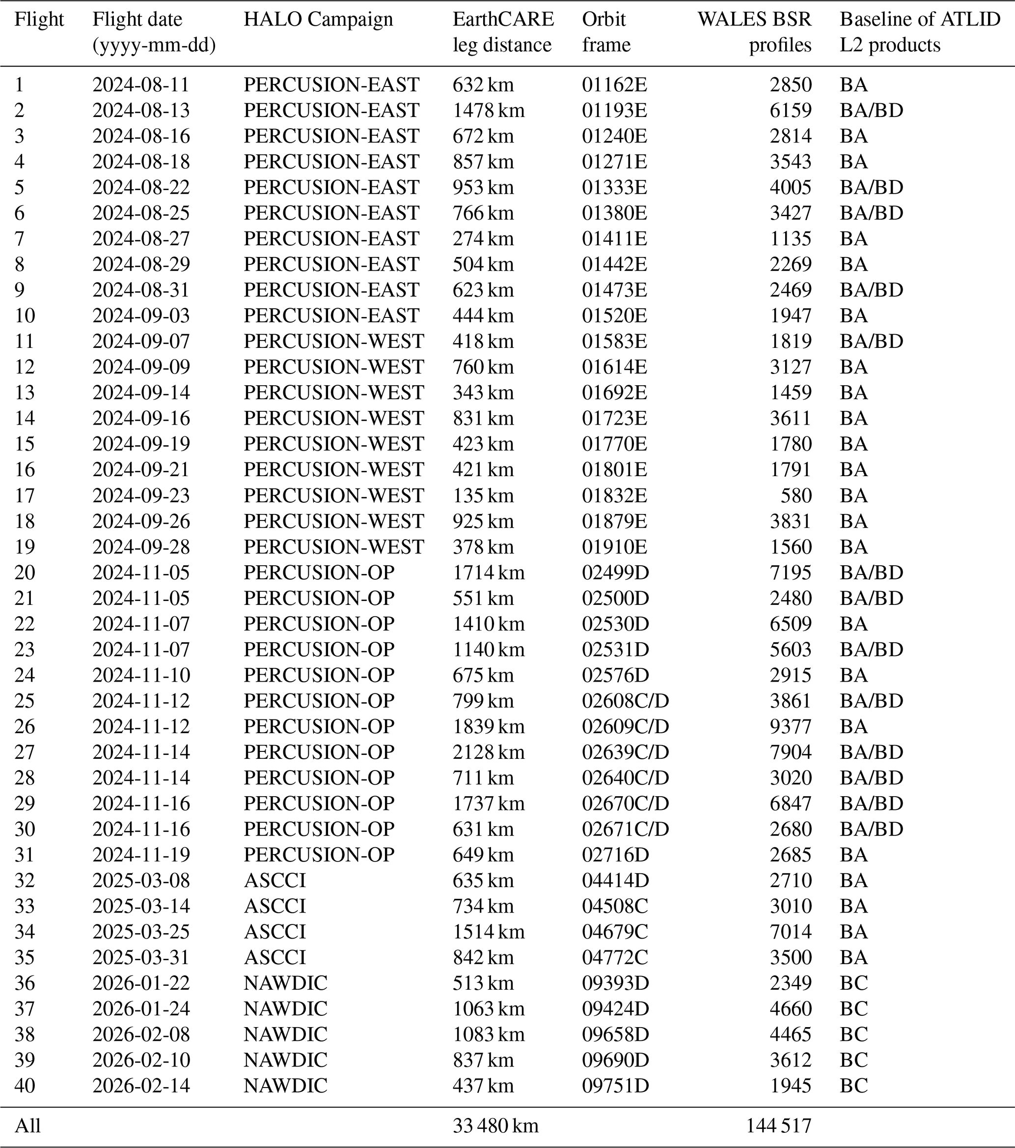
In this study, we use WALES BSR observations from 35 HALO research flights for which 40 coordinated EarthCARE underpasses were carried out during three airborne field campaigns in between August 2024 and February 2026 (see Fig. 1). The majority of underpasses (31) was taken in the course of the PERCUSION campaign in 2024 which was the German airborne contribution to the ORCESTRA campaign (ORganized Convection and EarthCARE Studies over the TRopical Atlantic; Stevens et al., 2026; see campaign website: https://orcestra-campaign.org/operation.html, last access: 27 May 2026). PERCUSION aimed for a better understanding of factors influencing organized convection in the tropics through enhanced airborne in-situ (e.g., dropsondes; Gloeckner et al., 2026) and remote-sensing measurements with HALO in coordination with EarthCARE satellite observations. To achieve this goal, HALO was equipped with an EarthCARE-like payload with WALES representing the ATLID instrument aboard EarthCARE, and a coordinated underflight was realized for every research flight (Groß et al., 2026). PERCUSION comprised three intensive observation phases, one in Cabo Verde (mainly August 2024, in this paper referred to as PERCUSION-EAST), one in Barbados (September 2024, referred to as PERCUSION-WEST), and one in Oberpfaffenhofen (November 2025, referred to as PERCUSION-OP). As illustrated by the flight tracks in Fig. 1, two EarthCARE underpasses could occasionally be achieved for some research flights during PERCUSION-OP due to the increased satellite orbital coverage towards higher latitudes. These locations were selected in order to obtain observations covering a broad spectrum of aerosol and cloud conditions representative of the tropics and the extratropics. In addition, four further EarthCARE underpasses were conducted at mid- and high latitudes (60–80° N) in the ASCCI (https://www.imkasf.kit.edu/english/4343.php, last access: 22 May 2026) campaign with HALO based in Kiruna (Sweden) in March 2025. ASCCI aimed to measure trace species in springtime Arctic polar vortex air in order to better understand their distribution and transport, and the chemical processes contributing to ozone depletion. Five further underpasses at mid-latitudes (40–60° N) were conducted during the NAWDIC (https://www.nawdic.kit.edu/, last access: 22 May 2026) field campaign. NAWDIC was an international multi-aircraft field study in January/February 2026 with HALO being based in Shannon (Ireland). The campaign was dedicated to advancing the understanding of mid-latitude atmospheric dynamics, with a particular focus on the mesoscale tropopause structure, dry intrusion airstreams, and their interaction with the planetary boundary layer. For each underflight segment, the goal was to position the satellite's overpass (see diamonds in Table 1) above the aircraft near the midpoint of the flight leg in order to achieve the best possible spatial and temporal collocation of the airborne and space-based observations. Across the three field campaigns, the 40 conducted underpass segments provide a large data set, spanning a cumulative flight distance of 33 480 km (Fig. 1, Table 1). Along this distance, WALES sampled more than 144 000 BSR profiles (averaged at 1 s temporal resolution) covering the Northern Atlantic from the tropics to the Arctic Ocean, as well as the Mediterranean Sea and central/northern Europe, providing a huge reference dataset available for the validation of ATLID products in a variety of sampled aerosol and cloud conditions (Groß et al., 2026).

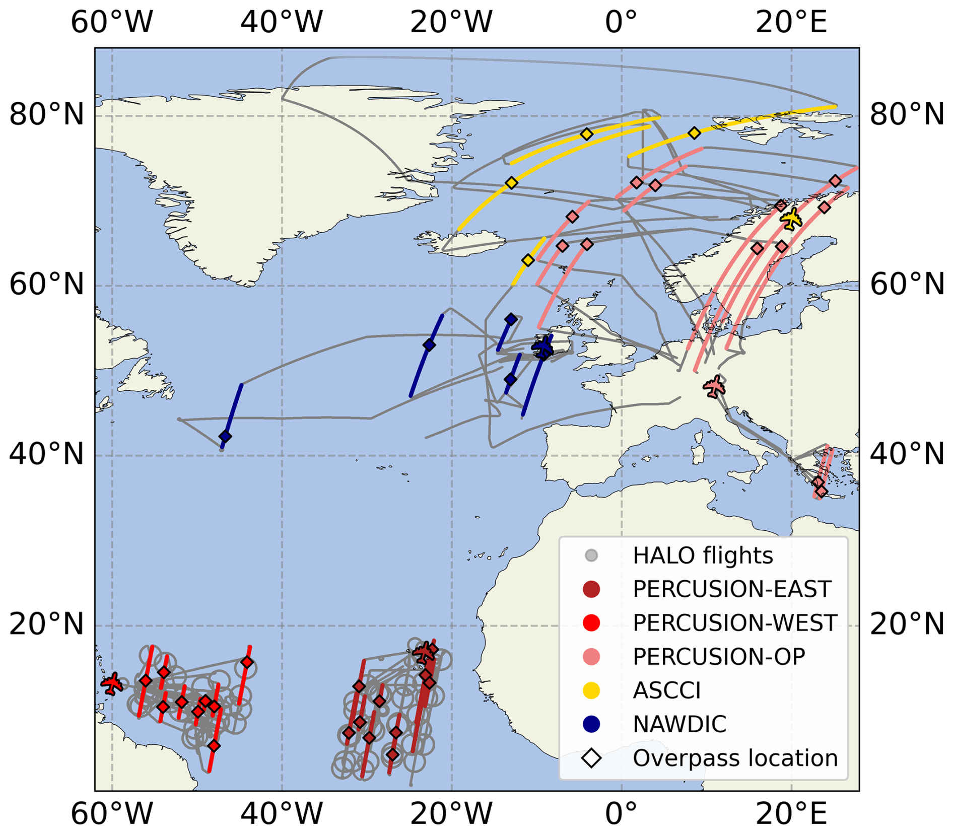
Figure 1 Overview of the flight tracks of the 35 HALO research flights (grey) and the associated 40 EarthCARE underflight segments carried out during the PERCUSION campaign parts (reddish), ASCCI (yellow) and NAWDIC (blue). The black diamonds in the colored segments mark the geographical location of the coordinated EarthCARE overpass. The aircraft markers represent the corresponding HALO aircraft base for each field campaign.

Table 1 Summary of the 40 coordinated EarthCARE underflight segments carried out during 35 HALO research flights. The corresponding flight dates, associated campaigns, the distance with collocated WALES observations along the EarthCARE ground track, orbit frame, the number of WALES BSR profiles (with > 1 km coverage) and the baseline of the ATLID Level 2 products evaluated in this study are shown.

2.1.2 Cloud pixel classification and cloud top height retrieval from WALES BSR data

The following paragraphs describe how the WALES BSR data set is applied to identify cloud pixels in order to generate a cloud mask for comparison with the ATLID Level 2 products A-FM, A-TC and A-CTH. A multitude of previous studies have demonstrated that lidar backscatter signals enable the discrimination of aerosols, clouds, and clear-sky conditions, typically based on threshold approaches (e.g., Winker et al., 2007; Liu et al., 2024) that account for variations in signal intensity arising e.g. from changes in atmospheric density. Winker et al. (2007) have demonstrated that clouds and aerosol layers can be effectively detected by applying range-dependent thresholds to BSR observations from the spaceborne lidar CALIOP (Vaughan et al., 2004). Height-dependent thresholds are also applied to the received backscatter signals from ATLID within the A-TC and A-CTH algorithms (Irbah et al., 2023; Wandinger et al., 2023). Since the retrieved BSR values also depend on wavelength of the applied lidar system, a careful selection of thresholds tailored to the WALES HSRL (providing BSR at 532 nm) is required. Previous studies have already successfully employed WALES BSR measurements for cloud identification, exploiting the distinct value ranges of BSR associated with clear-sky conditions, aerosols, ice clouds, and liquid clouds. For example, Gutleben et al. (2019) applied a comparatively high threshold (BSR > 20) to detect tropical boundary layer clouds and to effectively separate them from Saharan mineral dust (typically BSR between 1.5 and 6, occasionally up to 10), whereas Urbanek et al. (2017) and Dekoutsidis et al. (2024) used a lower threshold (BSR > 2) ensuring sensitivity to mid- and high latitude ice clouds. These studies demonstrate that WALES BSR-based cloud detection is effective for the detection of specific cloud types (ice or liquid clouds) but relies on case-dependent tuning. Due to the variable and partly overlapping BSR ranges of liquid clouds, ice clouds, and aerosols, and given that all of these features are expected in the dataset (Sect. 2.2), this study requires a generalized algorithm that is robust and sensitive to all cloud types across tropical and extratropical conditions, while remaining resistant to aerosol contamination such as Saharan dust.

In this study, a classification scheme is developed based on the range-resolved BSR from WALES, combined with temperature analysis data from the European Centre for Medium-Range Weather Forecasts (ECMWF) Integrated Forecasting System (IFS) (ECMWF, 2026). The inclusion of the IFS temperature data is motivated by the fact that cloud phase (ice, mixed-phase, or liquid) and, in turn, cloud optical properties are strongly temperature dependent (e.g., Hogan et al., 2003; Costa et al., 2017).

Thus, a temperature-dependent is applied to the WALES BSR data set for the cloud-or-no-cloud decision. At temperatures below 265 K, for which a rapid increase of the share of the ice-phase inside a cloud has been documented (e.g., Costa et al., 2017), pixels are classified as cloudy if the WALES BSR > 1.8. This threshold is motivated by the findings by Groß et al. (2014), who showed that this WALES BSR value coincides to conditions near or slightly above ice saturation (RHi ≥ 100 %) within cirrus clouds where ice particles measurably influence the surrounding water vapor field making BSR > 1.8 an appropriate lower boundary for cirrus detection. For temperatures above 265 K, where liquid, and mixed-phase clouds prevail (e.g., Costa et al., 2017) a higher threshold (BSR > 10) is applied for the cloud detection. This reflects the optical properties liquid clouds, which typically lead to rapid attenuation of the laser beam within a few range bins and high BSR. The higher threshold also avoids misclassification of optically dense aerosol layers, such as Saharan dust (Gutleben et al., 2019).

Cloud detection from WALES BSR profiles with 1 s horizontal resolution is performed using a moving 3 × 3 (horizontal × vertical) pixel window to ensure spatial consistency and to prevent isolated noisy pixels from being misclassified as clouds. For each window position, the temperature of the central pixel determines the applicable threshold. If the central pixel does not exceed this threshold, it is classified as non-cloudy. If it exceeds the threshold, the BSR values of the eight neighboring pixels are examined. Only if at least three neighboring pixels also exceed the same threshold, the central pixel is classified as cloudy; otherwise, it is classified as non-cloudy. The 3 × 3 window is shifted horizontally and vertically across the full lidar cross section of each underflight to generate a two-dimensional cloud mask (see Figs. 3b and 4b).

From this mask, the cloud top height is subsequently determined for each profile by scanning from top to bottom and identifying the uppermost pixel classified as cloudy. If this altitude coincides with the highest measured BSR value of a profile the cloud top detection is considered ambiguous (e.g., in case ice clouds are located at HALO flight level or just below the aircraft), and the cloud ceiling from this profile is rejected. Finally, both the WALES cloud mask and the WALES cloud top altitudes are interpolated onto the ATLID JSG (Eisinger et al., 2024) using the nearest-neighbor approach.

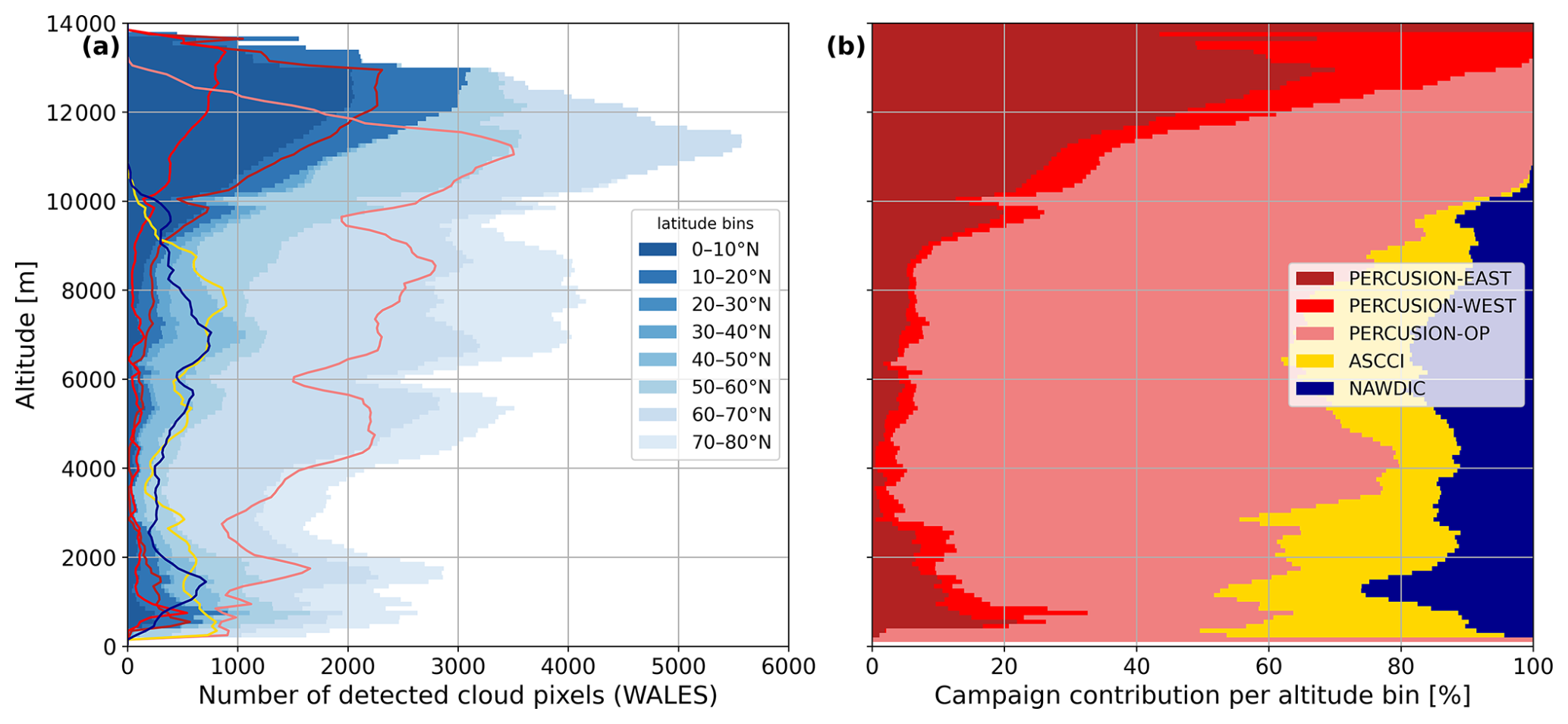
Figure 2 (a) Histogram of the cloud pixels (in 100 m altitude bins) determined from WALES for the full 40 EarthCARE underflights coloured with blueish contours by 10° bins of latitude, and number of cloud pixels observed per campaign (coloured lines), and (b) percentage contribution of each campaign per altitude bin.

Figure 2 illustrates the resulting cumulative distribution of cloud pixels for altitude bins determined from the WALES BSR observations for all 40 EarthCARE underflight segments and highlights the relative contributions from individual field campaigns. Figure 2a shows the detected cloud pixels from near the surface up to almost 14 km altitude revealing a multi-modal distribution characterized by several local maxima at different altitudes. The strongest peak occurs at altitudes between 10–13 km, reaching about 5500 cloud pixel counts, followed by a secondary maximum between 6 and 10 km with about 4000 counts. Further but weaker maxima appear at mid-levels (4–6 km; ∼ 3000 counts) and in the lower troposphere (0.5–2 km; ∼ 2500 counts). This multi-modal distribution reflects the variety of the sampled cloud types, including boundary-layer clouds (e.g., cumulus and stratocumulus fields), and especially cirrus layers observed across a wide range of latitudes which were targeted during the individual research flights. This is also expressed by the vertical positions of the maxima found at different altitudes for each campaign (lines in Fig. 2a). The highest clouds, with dominant peaks near 12–13 km altitude, are primarily observed during the tropical campaigns PERCUSION-EAST and PERCUSION-WEST, whereas for the extratropical campaign PERCUSION-OP the uppermost maxima are located at 9 and 11 km altitude. For the ASCCI and NAWDIC campaigns, the highest located maxima are found a bit lower (at ∼ 8 and ∼ 7 km, respectively), consistent with the generally reduced cirrus altitudes expected at higher latitudes and during spring or winter conditions (e.g., Stubenrauch et al., 2017). Mid-altitude clouds (3–5 km altitude) are detected in all campaigns but occur substantially less frequently, typically contributing only about 100–500 cloud pixels per campaign, except for the enhanced number of (> 1000) pixel counts during PERCUSION-OP. At low altitudes (< 2 km), each campaign exhibits a local maximum representing boundary-layer clouds; however, these local peaks are smaller by roughly a factor of 2–3 compared to the high-altitude maxima. Figure 2b presents the percentage contribution of each campaign per altitude bin, and shows that high-altitude cloud occurrence is largely dominated by the tropical campaigns, whereas low-level clouds are more evenly distributed among all campaigns.

2.2 Cloud parameters from ATLID (Level 2) single-sensor products

2.2.1 The A-FM feature mask

The single-sensor Level 2a Feature Mask product (A-FM; van Zadelhoff et al., 2023) provides an initial probabilistic detection of atmospheric features, based on backscatter signal properties (signal amplitude, noise characteristics) measured by ATLID's co-and cross-polar Mie channels and the Rayleigh channel. A-FM classifies particle features, including aerosols and clouds, and separates them from clear-sky conditions, surface returns, and fully attenuated range bins along each lidar profile. Feature detection is performed in two sequential stages. First, strong features (e.g., optically thick clouds and dense aerosol layers; A-FM retrieved values 8–10) are detected using an iterative hybrid median filtering approach that enhances spatial coherence while preserving sharp feature boundaries. In a second step, weaker features (e.g., thin clouds and low-altitude aerosol layers; values 5–7) are identified through iterative Gaussian convolution applied to the signal probability fields, allowing coherent low-signal structures to be distinguished from noisy clear-sky pixels (values 0–4). Regions classified as fully attenuated (−1) and surface returns (−3) are determined separately based on signal extinction and surface detection criteria. A-FM output is provided on the native ATLID grid, but here, we use the feature mask re-gridded to the JSG (1 km horizontally and 100 m vertically). The A-FM product furthermore serves as a structural input for the generation of different Level 2a and synergistic Level 2b products downstream in the processing chain (Eisinger et al., 2024). In particular, the A-PRO uses the feature mask, to retrieve vertically resolved aerosol and cloud optical properties, including extinction, backscatter, and depolarization product (A-EBD), aerosol properties (A-AER), ice microphysical estimates (A-ICE), and the ATLID Target Classification product (A-TC) (Irbah et al., 2023). Within A-PRO, the feature mask guides adaptive spatial smoothing and averaging strategies, ensuring preservation of cloud–aerosol boundaries and avoid mixing strong and weak scattering regimes. Details on the A-FM retrieval and the atmospheric feature flag definitions atmospheric features are provided in van Zadelhoff et al. (2023) or in the A-FM product data handbook available at: https://earthcarehandbook.earth.esa.int/catalogue/atl_fm__2a (date of last access: 25 August 2026).

2.2.2 The A-TC simple classification

The single-sensor Level 2a A-TC product (Irbah et al., 2023) provides a range-resolved classification of different particle types (i.e., aerosols, liquid and ice clouds) and is generated within the A-PRO processor (Donovan et al., 2024). The classification exploits ATLID depolarization measurements with retrieved optical properties (extinction, backscatter, lidar ratio, attenuated backscatter, along with associated uncertainties) and meteorological information from the X-MET product (e.g., temperature and tropopause height; Eisinger et al., 2024). Target classification is performed on vertically homogeneous layers identified within the extinction and backscatter retrieval modules (A-AER, A-EBD) which are the primary input fields for A-TC. The classification detection follows a decision-tree framework in which conditional thresholds based on e.g., depolarization ratio, extinction-to-backscatter ratio, particle extinction and temperature are applied to determine the most likely particle type. The classification algorithm consists of four sequential steps: (i) determination of homogeneous atmospheric layers, (ii) a simple classification ensuring robust identification with limited information, (iii) a detailed classification using the full set of available input parameters, and (iv) hybrid-mode smoothing to ensure spatial consistency. A-TC provides a range of target classifications, including a simple classification scheme, evaluated in this study as well as a more sophisticated classification incorporating aerosol typing. The simple classification separates between stratospheric aerosol and cloud features, liquid and ice clouds, tropospheric aerosols, clear-sky pixels, and surface and attenuated returns, but does not provide information on the aerosol type. The A-TC product serves as a key dataset within the Level 2 processing chain by translating lidar-retrieved optical properties into distinct aerosol and cloud classes, and is used as essential input for subsequent ATLID profile retrievals and synergistic radar–lidar products (Donovan et al., 2024). A detailed description of the A-TC target classification retrieval is provided by Irbah et al. (2023).

2.2.3 The A-CTH cloud top height

The single-sensor cloud top height product A-CTH (Wandinger et al., 2023) provides the geometric top altitude of the uppermost cloud detected along the ATLID field of view. The A-CTH retrieval is performed by the A-LAY processor for retrieved profiles identified as cloud and uses the Level 1b co-polar Mie backscatter signal resampled onto the JSG together with auxiliary information including surface altitude from the A-TC product and tropopause height from the X-MET product. Cloud top detection is performed based on a wavelet covariance transform (WCT) approach. The WCT identifies sharp vertical gradients in the ATLID co-polar Mie backscatter signal by correlating the signal with a Haar wavelet function, while thresholds are adapted to the local signal-to-noise ratio, altitude, and horizontal averaging scale, with the goal to allow a robust identification of cloud tops even under low-SNR conditions (Wandinger et al., 2023). It should be noted that the A-CTH cloud top height product is fully independently generated from the retrievals of A-FM and A-TC. The A-CTH product is stored in a layer-resolved format and serves as a key input for the generation of the synergistic ATLID-MSI cloud top height (AM-CTH) product (Haarig et al., 2023). More details on the A-LAY and the A-CTH algorithm are given by Wandinger et al. (2023).

3 Example cross sections for a tropical and an extratropical case

Figure 3 presents an example EarthCARE underflight conducted on 7 September 2024 during the PERCUSION-WEST campaign, when HALO flew a south–north transect in the tropical Atlantic departing from Barbados. This case was selected because it features complex aerosol and cloud conditions, in particular a well-defined, extended ice cloud field observed by both instruments, enabling a consistent comparison. The time–altitude cross section of the WALES BSR (Fig. 3a) reveals a variety of structures characterized by elevated values (BSR > 1.8), indicating the presence of cloud or aerosol particles, while lower values (BSR < 1.8) correspond to regions of low particle content. Frequent structures in enhanced backscatter above 6 km altitude indicate the strong presence of different ice clouds structures. A distinct cloud field is observed near 13 km altitude, which is optically thick in the vicinity of the EarthCARE underpass and becomes increasingly fragmented as well as vertically and optically thinner toward the northern part of the flight leg. Very large BSR values (BSR > 6) at lower altitudes furthermore reveal the presence of optically thick cloud structures, for example patchy mid-level clouds near the underpass at about 5 km altitude. At lower altitudes, large BSR values frequently aligned near 1 km indicate the presence of small-scale cloud structures, particularly at the beginning and end of the flight leg. In addition, slightly elevated low-level cloud fields (2–4 km altitude) are detected between 170 and 320 km along the flight track. Another notable feature is an extended layer of intermediate BSR values (1.8 < BSR < 6) within the lowest 3 km, suggesting the presence of aerosols attributable to Saharan dust, within which denser cloud patches (BSR > 10) are embedded. Figure 3b shows the corresponding WALES cloud mask, capturing the main cloud features identified in the BSR cross section, including high-level, mid-level, and low-level clouds. It should be stressed that none of the pixels associated with the Saharan dust layer are incorrectly classified as clouds by our developed cloud detection algorithm.

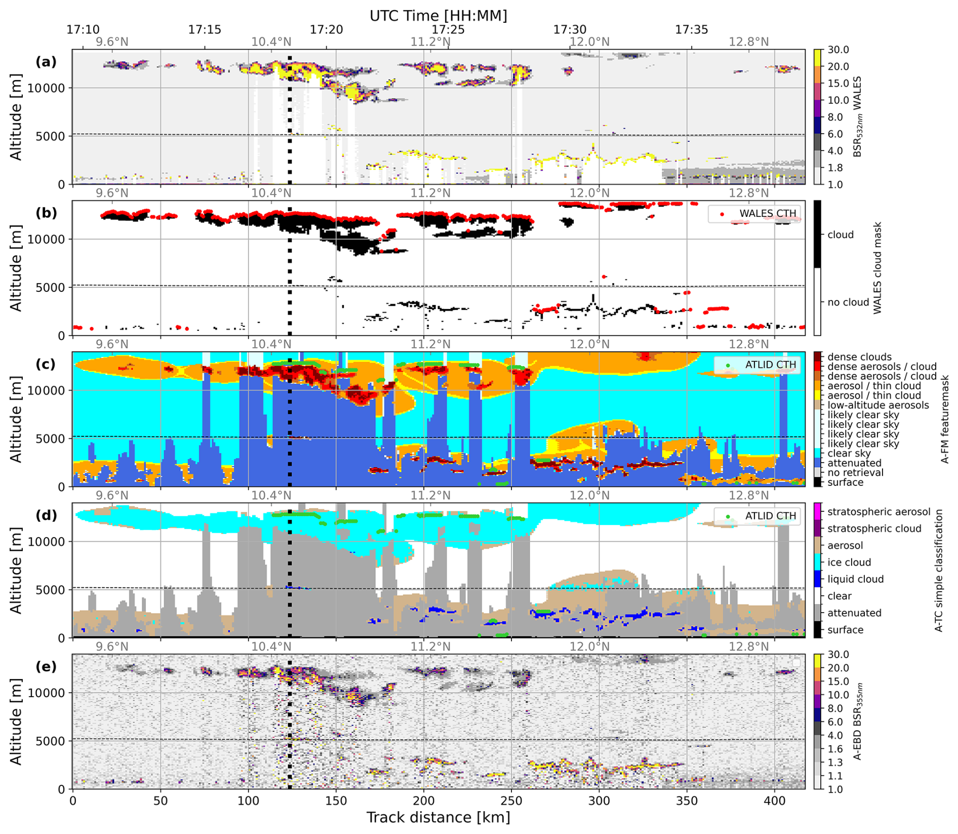
Figure 3 Time-altitude cross sections for the research flight on the 7 September 2024 from Barbados (PERCUSION-WEST) of (a) the BSR measured from WALES, (b) the cloud mask (black contours) and the top altitude of the uppermost cloud (red dots) as determined from WALES BSR, (c) the feature mask of the A-FM product, (d) the simple classification of the A-TC product, and (e) the ATLID BSR from A-EBD. The top altitude of the uppermost cloud from the A-CTH product is shown in panels (c) and (d) with green dots. The vertical black dashed lines illustrate the location of the EarthCARE underpass by the HALO aircraft. Note that the A-TC/A-FM atmospheric features are only displayed up to the altitude bins where WALES BSR measurements are available, close to the HALO flight altitude (horizontal black line). The horizontal thin dashed black lines (a–d) depict the IFS 0 °C isotherm. All ATLID Level 2 products shown represent baseline BA.

Figure 3c displays the feature mask provided by the A-FM product for the example underflight. Overall, the vertical and horizontal distribution of optically dense classified cloud features (uppermost three flags, reddish colors in Fig. 3c) in A-FM agrees well with the WALES cloud mask in terms of altitude ranges and general shape of the clouds. A-FM feature flags representing thin aerosol or thin cloud (orange and yellow in Fig. 3c) form a coherent cloud layer between 10 and 13 km altitude, covering nearly the entire transect. In contrast, this corresponding cloud structure in the WALES mask appears more complex, fragmented, and less vertically thick. This fragmented structure is covered by the A-FM dense cloud features (Fig. 3c) and is consistent with the structure of the BSR from the Level 2 A-EBD product (Fig. 3e). Figure 3d illustrates the simple classification provided by the A-TC product. This mask fundamentally distinguishes between liquid clouds, ice clouds, and aerosols. In general, the A-TC simple cloud distribution is consistent with the WALES mask, with liquid cloud classifications predominantly occurring at low altitudes and corresponding to the small-scale cloud features observed by WALES. Similar to the optically thin and thick feature in A-FM, A-TC classified a coherent layer of ice clouds extending along the entire cross section between 10 and 13 km altitude. A-TC furthermore shows an aerosol layer within the lowermost 3 km covering almost the entire cross section. Between 270 and 350 km along the flight track, this aerosol layer forms a plume-shaped structure reaching altitudes of up to ∼ 6 km. Within this structure, A-TC classifies some pixels as ice clouds (which are not contained in the WALES cloud mask), and conversely aerosol pixels appear occasionally at the edges of the ice clouds.

The cloud top height of the uppermost clouds derived from the A-CTH product is overlaid in Fig. 3c and d (green dots). A-CTH shows cloud tops associated with high-, mid-, and low-level clouds, and occasionally detects cloud tops above HALO's flight altitude that are not detectable by WALES.At high altitudes, A-CTH and WALES top heights are found at comparable altitudes, whereas for low-level clouds, A-CTH cloud tops appear frequently lower than those derived from WALES, a finding examined in more detail in Sect. 4.3. Notably, A-CTH cloud tops are frequently located at the upper transition between thick and thin features in A-FM and lie within regions classified as ice cloud by A-TC. At altitudes below approx. 6 km, A-CTH cloud-top heights agree closely with A-TC liquid cloud and with A-FM cloud and dense-features. It should be noted that A-CTH does not produce a cloud top altitude in cases of Saharan dust, where the A-TC classification provides an ice cloud pixel.

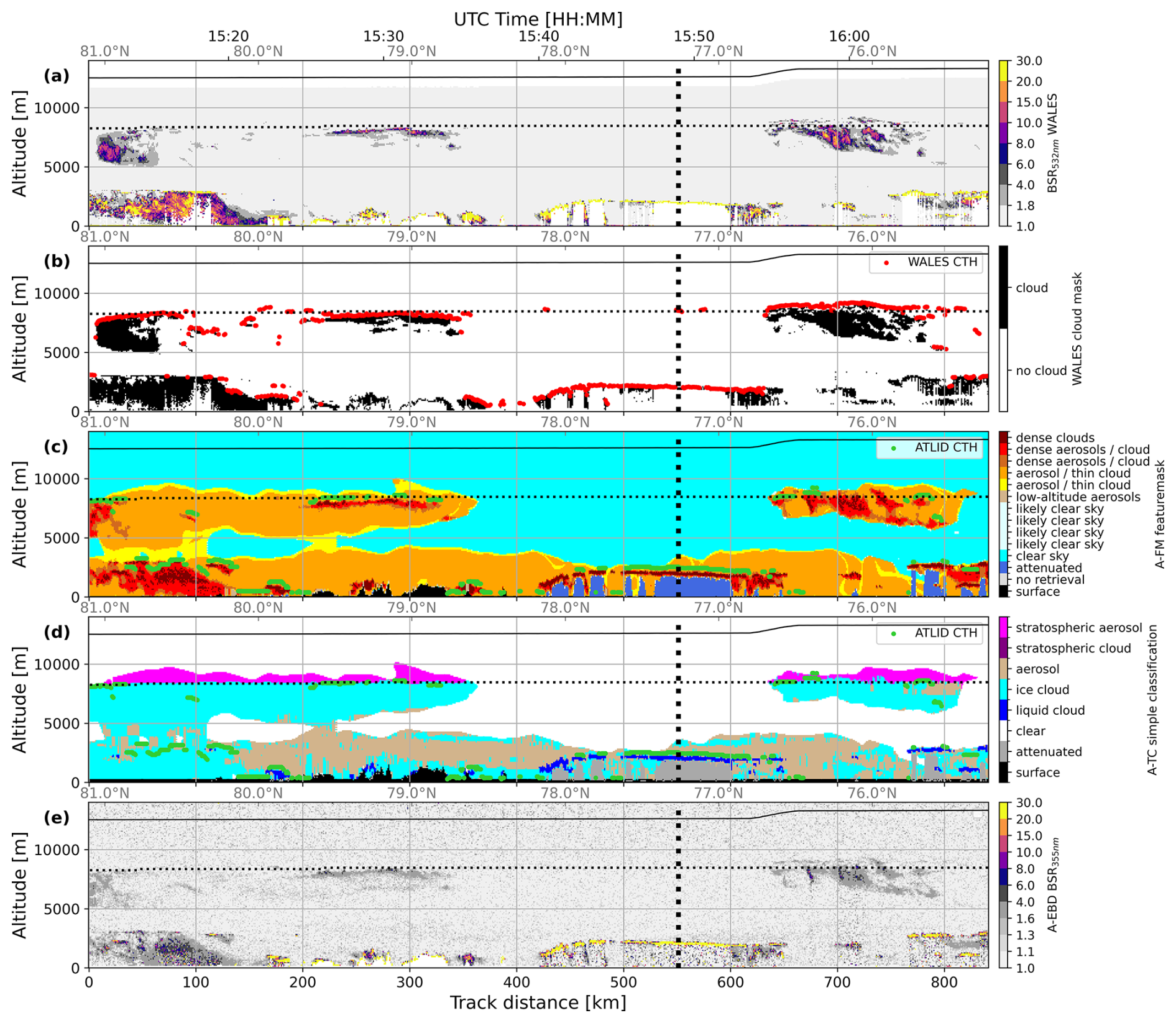
Figure 4 Time-altitude cross sections with the same parameters as for Fig. 3, but for the research flight on the 31 March 2025 from Kiruna (ASCCI). The horizontal black dashed line in panels (c)–(e) represents the tropopause altitude provided from A-EBD. All ATLID Level 2 products shown represent baseline BA.

A second case study is presented to illustrate an EarthCARE underflight on 31 March 2025 during the ASCCI campaign in extratropical conditions (Fig. 4). During this flight, HALO performed a north–south transect across Svalbard and the Arctic Ocean, targeting both high- and low-level cloud systems in a cold tropospheric environment with temperatures below 0 °C down to the surface. The WALES BSR cross section and the corresponding cloud mask (Fig. 4a–b) reveal high-altitude cloud layers between approximately 5 and 9 km altitude during the first half and toward the end of the flight leg. In addition, optically dense cloud fields with cloud tops below about 3 km altitude are also a characteristic feature of the scene.

Consistent with the previous case (Fig. 3), the high-level clouds are also captured by the A-FM and A-TC products and classified as thick features (A-FM; Fig. 4c) and ice clouds (A-TC; Fig 4d), respectively, but again, compared to the WALES cloud detection, the cloud features have a greater vertical extent in the ATLID Level 2 products. Interestingly, the cloud formation between 6–10 km altitude in the A-TC product is subdivided near the roughly constant tropopause level at 8 km altitude into an ice cloud feature below and a stratospheric aerosol feature above. Another prominent feature occurs within the first 100 km of the transect, where WALES observes (ice) clouds between 6–8 km altitude and again below approximately 3.5 km altitude, separated by a cloud-free layer. In contrast, both A-FM (Fig. 4c) and A-TC (Fig. 4d) depict these layers as a vertically continuous feature (including aerosol pixels) extending through much of the lower 8 km of the profile. Near the underpass location (between 450–600 km along track), an extended cloud field with a relatively uniform cloud top height around 3 km is observed consistently in WALES, A-FM, and A-TC, below which the strong attenuation suggests the presence of a partly liquid-phase cloud. Furthermore, both A-FM and A-TC display a coherent layer of aerosol or thin cloud features within the lowest 4–5 km of the cross section. Regarding the A-CTH product, it is noticeable that the retrieved cloud top heights generally agree well with the heights of the liquid cloud pixels (A-TC; Fig. 4d) as well as with the two highest-ranked flags in A-FM. However, in the extended ice cloud fields shown in A-TC, A-CTH does not consistently retrieve cloud tops at the geometric upper boundary. Instead, cloud top heights are mainly assigned to the densest pixels (indicated by the flags 9 and 10 in A-FM) within these ice clouds, which overall results in a high correlation with the WALES cloud top heights. In addition, cases of notably low A-CTH cloud top heights (< 200 m) are again observed which is discussed in Sect. 5.

4 Statistical validation of cloud macrophysical properties from ATLID Level 2 products A-FM, A-TC and A-CTH

The two case studies presented in the previous section are intended to provide an initial overview of the WALES BSR observations and cloud mask, as well as the ATLID Level 2 data products A-FM, A-TC, and A-CTH for aerosol and cloud conditions in an example tropical and extratropical flight. Overall, the ATLID products demonstrate a generally realistic representation of various cloud features; however, there are indications of systematic discrepancies when compared to the corresponding WALES observations. In the following section, these differences are investigated in a more comprehensive and statistical manner based on the full dataset. We first focus on the cloud frequency (cloud pixel distribution) from the simple classification of the A-TC product and the feature mask of the A-FM product in a flight-by-flight analysis as well as in a statistical analysis of all flights (Sect. 4.1). This is followed by a statistical comparison of the cloud top heights detected from WALES and provided by the A-CTH product (Sect. 4.2).

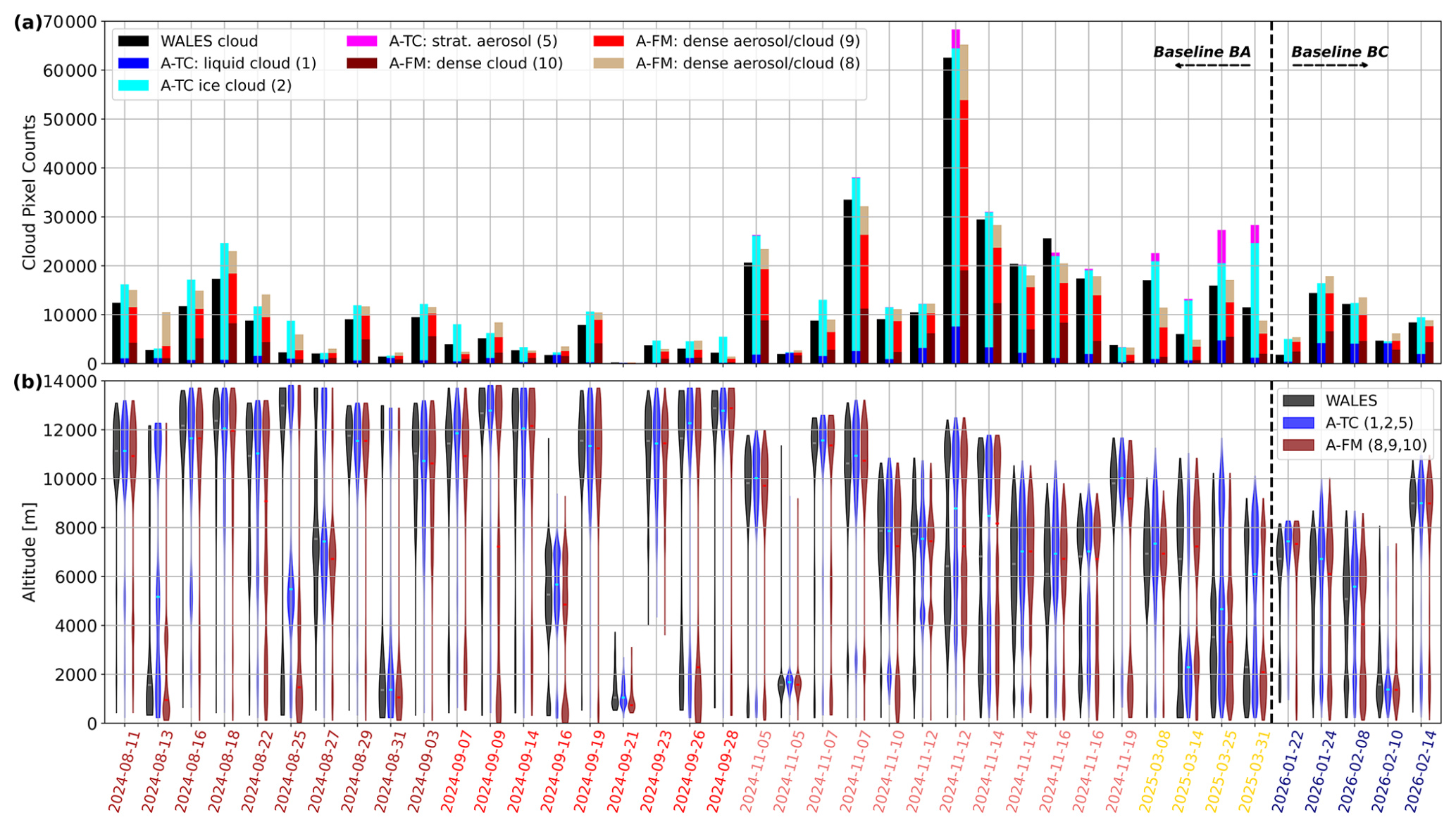
Figure 5 (a) Number of cloud pixel counts per research flight given as bar plots for WALES, A-TC's simple classification (flag 1, 2, 5), and the A-FM's feature mask (flag 8–10) with the same colouring as in Fig. 3. Panel (b) illustrates the vertical distribution of cloud pixels as violin boxplots for WALES (black), A-TC (blue) and A-FM (red). The horizontal bars inside the violins represent the median. The colouring of the x-axis labels corresponds to the different field campaign with the same color-coding as in Fig. 1.

4.1 Validation of the Level 2a classification products A-FM and A-TC

Figure 5 provides an overview of the variability in detected cloud pixels and their corresponding altitude as violin distributions across the individual research flights and campaigns for WALES and the ATLID Level 2 products. The number of cloud pixels detected by WALES varies strongly among the flights (Fig. 5a), ranging from about 1000 to nearly 70 000 pixels. This large spread is primarily related to the variable length of underflight segments (see Table 1), as well as the differing cloud and aerosol conditions targeted and encountered during the missions. Both the A-TC (liquid and ice cloud flags) and the A-FM (dense cloud flag 10, and the two dense cloud/aerosol flags 8 and 9) products generally reproduce the magnitude of this variability in cloud pixel counts across the flights well. However, both satellite products clearly show higher pixel counts compared to WALES for the majority of the flights (A-TC: 37 of 40 flights, A-FM: 30 of 40 flights). For approximately half of the flights, both products show good agreement with WALES, with relative deviations within ±25 % (17 flights for A-TC and 20 flights for A-FM). A small number of flights (6 in A-TC, 3 in A-FM) have a substantially higher number of pixels (by a factor of > 2) compared to WALES, but these are cases in which generally fewer cloud pixels were observed. Cases of pronounced overestimations are found to occur especially during the extratropical campaigns between November 2024 (PERCUSION-OP) and March 2025 (ASCCI). These flights are associated with an enhanced occurrence of the A-TC ice cloud flag and, in particular, the stratospheric aerosol flag, which may be related to tropospheric ice cloud features (cf. Fig. 4). It should be noted that during the extratropical flights in 2026 (NAWDIC, baseline: BC), no pixel counts associated with the stratospheric aerosol flag could be found, which will be discussed in Sect. 5.1. An additional noteworthy result is that the cumulative pixel counts of two uppermost flags (9, 10) in the A-FM product are often in good agreement with the WALES pixel counts.

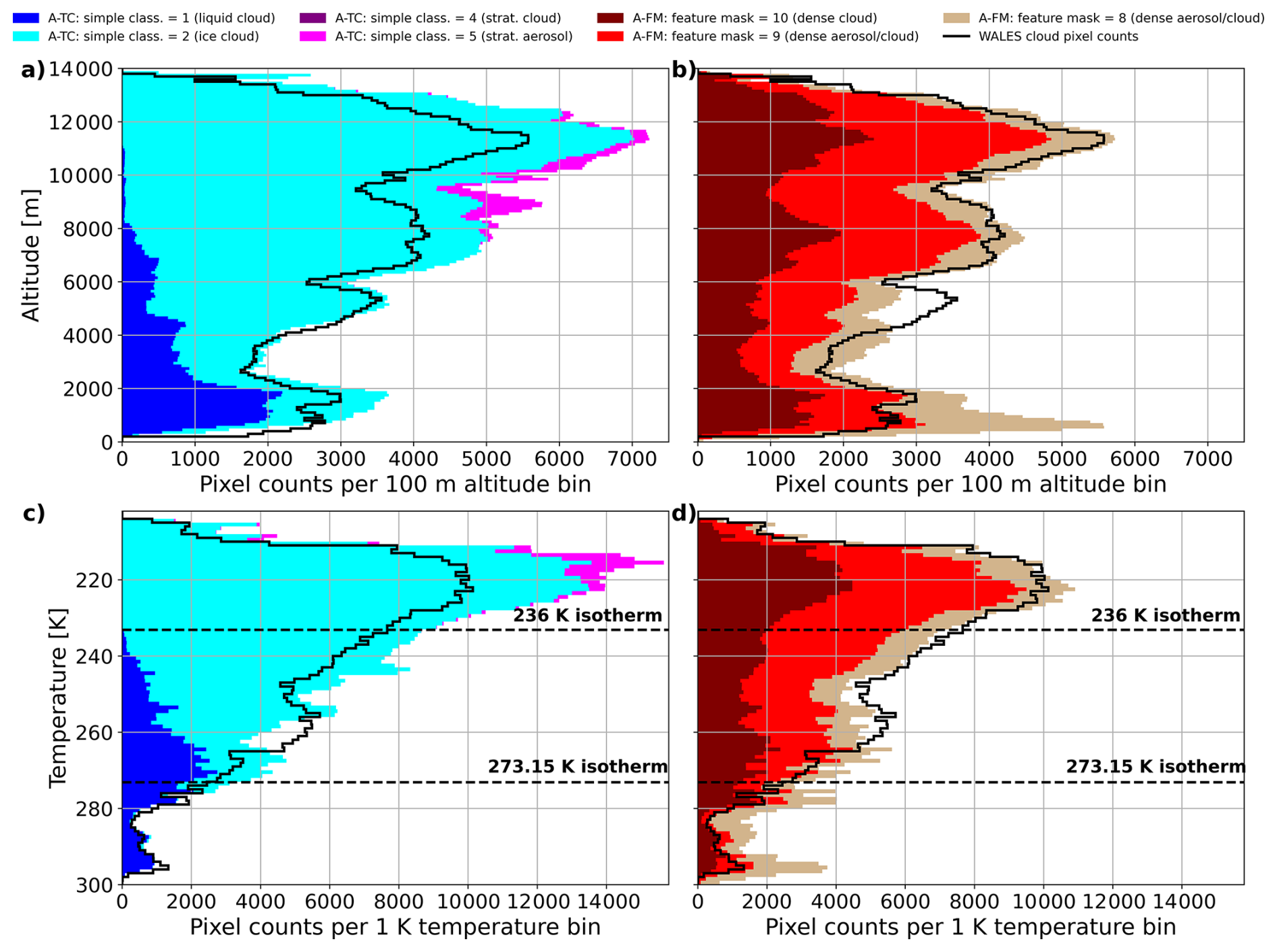
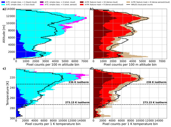
Figure 6 Vertical distributions of cloud pixels determined from WALES (black step histogram) for the 40 full EarthCARE underflight segments. Histograms are shown for 100 m altitude bins in panels (a) and (b) and for 1 K temperature bins in panels (c) and (d). The stacked colouring in panels (a) and (c) represent the pixel counts from the A-TC simple classification, whereas in panels (b) and (d) the colouring stacked here as well shows the distribution of atmospheric features classified by the A-FM product (see legend).

Figure 5b shows, the vertical distribution of detected cloud features in WALES, A-TC, and A-FM represented as violin distributions. Based on the WALES observations (black violins), most flights exhibit either unimodal or bimodal vertical distributions demonstrating that low-level, mid-level and high-level clouds are captured by the observations. The shape of the violins generally indicates that a dominant fraction of the detected clouds occurred at high altitudes. During the tropical flights in August and September 2024, cloud pixels are located between about 10–14 km altitude. For the subsequent extratropical campaigns, the cloud pixels are located at lower altitudes and show a larger variability (about 7–12 km altitude) which is consistent with Fig. 2. In addition to these high-level clouds, smaller fractions of clouds are frequently detected at lower altitudes, including mid-level clouds between approximately 4 and 7 km and, in some cases, clouds within the lowest 2 km of the atmosphere. Overall, the vertical distributions derived from WALES, A-TC (blue violins), and A-FM (red violins) show a broadly similar structure for most flights. However, the A-TC and A-FM distributions occasionally exhibit trimodal structures that are not similarly present in the WALES observations, which may point to cases of either cloud/aerosol misclassifications (e.g., 13 August 2024; 25 August 2024 in Fig. 5b), or situations of low representativeness due to cloud field drifting into/out of the scene and thus are captured by only WALES or ATLID (e.g., 12 November 2024; 19 November 2024 in Fig. 5b).

Figure 6 shows the vertical distribution of detected features from the two ATLID products A-TC (Fig. 6a, c) and A-FM (Fig. 6b, d), displayed as stacked histograms with different colors separated by the respective classification masks (see legend). The distribution of cloud pixels detected from the WALES BSR dataset is shown as a black line. Overall, the cumulative distributions from both ATLID products follow the vertical cloud pixel distribution observed by WALES. In both satellite products, pronounced maxima occur between approximately 11–13, 6–10, and 1–2 km altitude in correspondence to the WALES observations (Fig. 6a, b). The vertical distributions with respect to temperature (Fig. 6c, d) show a more uniform shape, with a clear maximum in pixel counts (10 000 in WALES) at around 220 K which confirms the strong presence of ice clouds in the dataset. The cloud pixel counts then steadily decline towards higher temperatures up to 280 K, and exhibit another small local maximum at 295 K (1500 counts), which is related to the frequently captured (liquid) low-level clouds in the tropics. This distribution is also represented by A-TC and A-FM.

The A-TC product consistently shows higher cloud pixel counts compared to WALES at nearly all altitudes (Fig. 6a). Differences are most pronounced above 6 km and below 2 km, where A-TC exceeds WALES by about 20 %, while deviations in the intermediate layer (2–6 km) remain very small (< 5 %). Figure 6b indicates that the majority of these higher cloud detections in A-TC occur at temperatures below 250 K, whereas agreement between A-TC and WALES is very good at temperatures above 273.15 K. Notably, an enhanced number of stratospheric aerosol counts are found in A-TC above 6 km (Fig. 6a), and these potentially misclassified aerosols are exclusively found at temperatures below 236 K. In addition, an enhanced occurrence of higher A-TC cloud pixel counts is observed in the temperature range of approx. 265–275 K. It is furthermore noted, that WALES detects slightly more cloud pixels than A-TC at very low altitudes (< 1 km, above 290 K), even though a small number A-TC of likely misclassified ice cloud pixels are found at temperatures above 273.15 K.

The A-FM product does not provide a strict separation between cloud and aerosol features, but its pre-classified feature flags serve as input for subsequent products (e.g., A-TC). Considering the uppermost three feature classes (flags 8–10; optically dense features, see legend), A-FM (Fig. 6c) shows good agreement with WALES above 6 km (and at temperatures < 250 K; Fig. 6d), with only small deviations (< 5 %). Lower-ranked A-FM features (i.e., values 5 and 6, associated with optically thin features) lead to a substantial increase in the number of detected pixels which is likely related to the presence of aerosols (indicated in Appendix B). At lower altitudes between 4 and 6 km, WALES detects a higher fraction of cloud pixels by about 30 %, while below 4 km, A-FM shows an increased number of classified features, particularly associated with optically dense aerosol or cloud (flag 8). This is reflected in a pronounced peak in the A-FM distribution around 1 km altitude (around 290 K, Fig. 6d), where A-FM pixel counts exceed WALES pixels by about 100 %.

4.2 Validation of A-CTH cloud top altitudes

Figure 7 illustrates the correlation between cloud top altitudes detected by WALES and A-CTH (Baseline BA and BC) for the full multi-campaign dataset. Figure 7a shows that most cloud top observations occur along the diagonal, and that the majority of data points exhibit deviations of less than 2 km (dotted black lines in Fig. 7). Within this range several clusters of enhanced counts (red to dark red coloring) can be identified. Smaller clusters occur near cloud-top altitudes of approximately 3–5 km altitude, while more extended clusters are located between about 1–3, 8–11, and 12–14 km altitude. Figure 7b provides the median latitude per bin allowing to link these clusters to distinct cloud structures occurring at different latitudes. The cluster between 8 and 11 km is primarily associated with (ice) clouds observed at mid-latitudes (40–50° N) and high latitudes (60–80° N), whereas the cluster between 12 and 14 km mainly corresponds to clouds observed at mid-latitudes (50–60° N) and in the tropics (< 20°). One finding is that most of these clusters are located slightly above the diagonal line, indicating that the A-CTH cloud top altitudes are generally slightly higher than those detected by WALES. A striking exception is the frequent detection of very low altitude cloud tops (< 0.5 km) in A-CTH where WALES provides cloud tops distributed between 0.5 and 14 km which may hint to misdetections of A-CTH products at these altitudes (already indicated by Figs. 3, 4 and discussed in Sect. 5). Figure 7b clearly shows that such potential misdetections are found in both the tropics and in the extratropics.

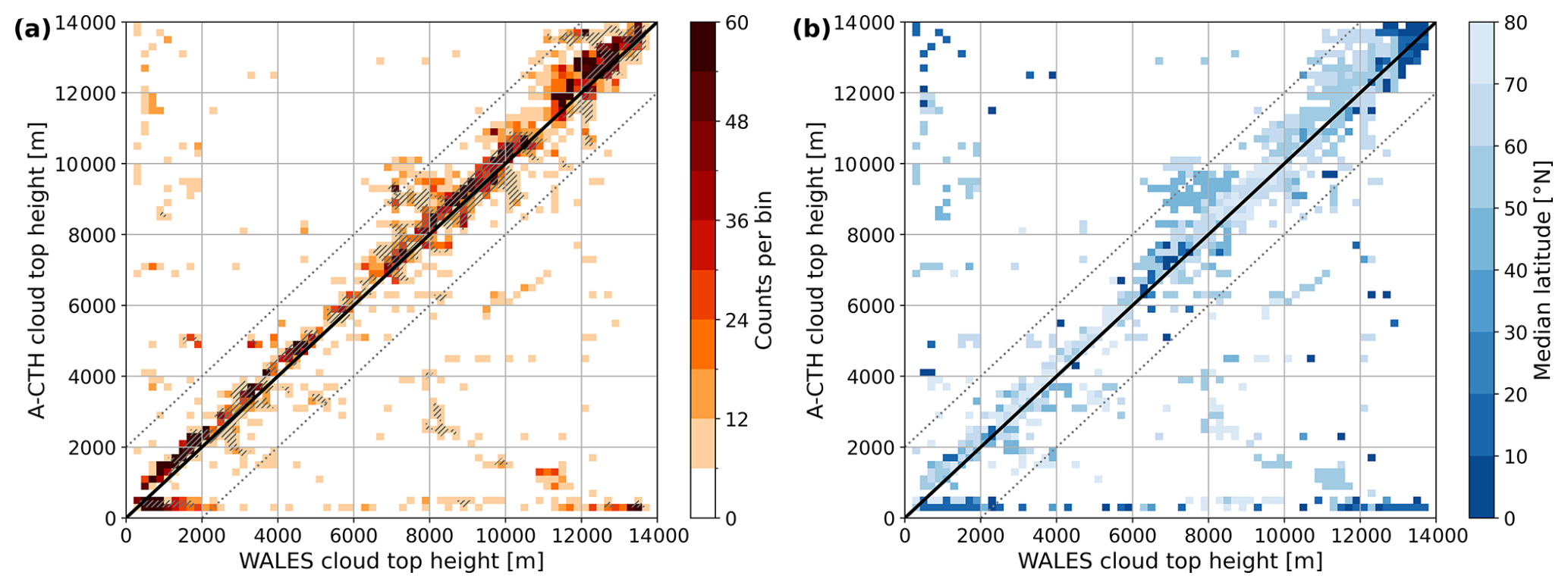
Figure 7 Correlation between WALES and A-CTH cloud top altitudes using 100 m bins for the full multi-campaign data set. In panel (a), colors indicate the number of cloud top detections per bin, while grey hatched bins include the 75 % of detections closest to the EarthCARE underpass (within ±560 km). Panel (b) shows the median latitude per bin. The solid black diagonal line indicates perfect agreement between WALES and A-CTH cloud top altitudes, and the grey dotted lines denote deviations of ±2000 m.

In addition to the main clusters near the diagonal, numerous isolated bins with low counts are found outside the ±2 km deviation interval, indicating cases with substantially larger cloud top height differences between the two datasets which may be related to cloud edge uncertainties or to spatial mismatch. To investigate the potential influence on the spatial mismatch, Fig. 7a uses hatching to indicate bins that include observations within a radius of about 40 min. of the satellite underpass location, representing 75 % of the data counts. Non-hatched bins correspond to cloud-top detections located beyond this time difference, implying reduced spatiotemporal collocation between ATLID and WALES measurements. Notably, many isolated bins are non-hatched, suggesting that the observed cloud top height differences of the isolated bins may be partly attributable to reduced representativeness. In contrast, most of the clusters along the diagonal line frequently contain hatched bins, indicating a high degree of spatial collocation between ATLID and WALES measurements. However, clusters of poor collocation (i.e., non-hatched bins between 11 and 13 km altitude) are also found along the diagonal, suggesting that cloud-top detections with reduced collocation should not generally be excluded from the validation, as they may still provide useful information. Figures 6 and 7 illustrate that the cloud pixels detected by WALES form distinct clusters across different latitudes, temperatures, and altitudes, thereby representing a variety of distinct cloud regimes. In the following, the dataset is coarsely sub-categorized based on temperature to assess the accuracy of A-CTH cloud top heights for different cloud regimes and with respect to distance to underpass. Figure 8a presents violin distributions of cloud top geometric heights measured by WALES, with the data categorized according to temperature. Specifically, we distinguish between warm clouds (temperature above the freezing level, T > 273.15 K), mixed-phase clouds in tropical and extratropical regions (273.15 K > T > 236 K; latitude: 30 and < 30° N), and ice clouds (T < 236 K).

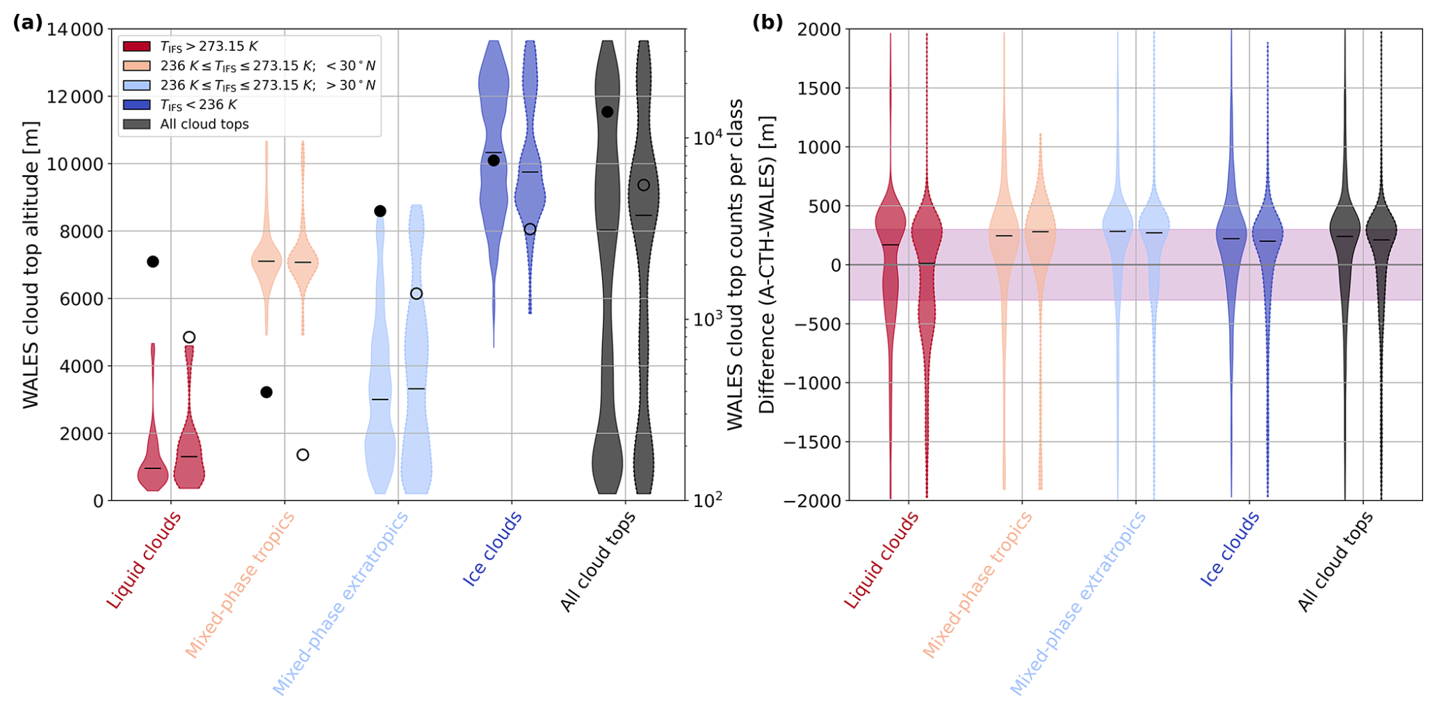
Figure 8 (a) Cloud top height distribution shown as violin plots for WALES observations colored by distinct defined cloud class (liquid clouds, extratropical and tropical mixed clouds, ice clouds and for the full data set; see legend). For each class the solid-framed violins represent data for the full cross underpass segments, while the dashed-framed violins (the right violins of each pair) represent data within ±10 min. to the EarthCARE underpass. The counts per class (black filled for full data set, unfilled for ±10 min around underpass location) is shown with respect to the secondary, logarithmic-scale y-axis. (b) Differences in cloud top height between WALES and A-CTH (A-CTH − WALES-CTH), shown as violins for the same classes as in panel (a). The magenta shading in panel (b) depicts the ±300 m accuracy requirement according to Wehr (2006) and Wandinger et al. (2023).

The liquid clouds exhibit a comparatively narrow distribution, with cloud top altitudes predominantly confined to the lowest 2 km of the atmosphere. In contrast, mixed-phase cloud tops in both tropical and extratropical regions show a much broader distribution. Tropical mixed-phase clouds display a unimodal structure, with cloud tops primarily located between 6 and 8 km altitude, whereas extratropical mixed-phase clouds exhibit a trimodal distribution spanning from approximately 0.2 up to 9 km. Ice clouds are found at higher altitudes, shaping a broad distribution covering an altitude range extending roughly from 7 to 14 km. The black violin, representing the full dataset, reveals a pronounced trimodal structure, reflecting the frequent occurrence and detection of all three cloud regimes. It should be noted that the violin distributions (Fig. 8) include only cases where the cloud top heights from WALES and A-CTH differ by less than 2 km, in order to ensure that large deviations (e.g., at cloud edges or due to drifting cloud fields) do not influence the statistics. Figure 8b shows the differences between A-CTH cloud top heights and those derived from the WALES cloud mask. The distribution of cloud top differences for the full dataset spans a wide range, with the majority (about 80 %) of the differences lying within ±500 m. Overall, the distribution is shifted toward higher cloud top altitudes in A-CTH, with a median at almost +300 m. Roughly 50 % of the differences fall within the target accuracy interval of 300 m defined for A-CTH. A systematic tendency toward overestimation of cloud top heights is consistently observed for ice clouds as well as for tropical and extratropical mixed-phase clouds, all of which exhibit relatively uniform distributions with medians located around +300 m. An exception is found for the category of warm (liquid) clouds, where A-CTH tends to underestimate cloud top heights on average. Interestingly the distribution of differences in this category is bimodal, with one maximum similar to the other categories at slightly above +300 m, and a broader secondary maximum ranging between −200 and −600 m which may point to a potential false cloud top detections in A-CTH near surface in this category.

To further assess how the findings on A-CTH cloud top height accuracy depend on the distance to the EarthCARE underpass, Fig. 8 additionally shows dashed violin plots for each category, including only cloud tops observed within ±10 min of the underpass. This subsetting reduces the sample size by roughly one-half to two-thirds per category, but for the remaining data a higher representativeness is to be expected. Nevertheless, the resulting distributions remain largely robust. In particular, extratropical mixed-phase and ice clouds exhibit more clearly defined distributions (Fig. 8a), reflected in a more distinct trimodal structure compared to the full dataset. Importantly, the main findings regarding cloud top height differences remain nearly unchanged, with all categories showing consistent tendencies toward a systematic overestimation of cloud top heights of a similar magnitude. However, for extratropical mixed-phase and ice cloud classes, the median differences shift slightly closer to zero when considering the subset with the stricter temporal collocation. For the liquid cloud, and the tropical mixed-phase class, the magnitude of the median difference slightly increases.

4.3 Statistical comparison of A-TC and A-CTH between Baseline BA and BD

To investigate potential improvements in recent baseline revisions, the A-TC and A-CTH products are retrieved for 12 cases (see Table 1) from the preoperational baseline dataset BD, which is being considered as a candidate for the next major baseline (version CA). Figure 9 A-TC cloud pixels distributions binned in 1 K temperature intervals for 12 cases for the baseline BA (Fig. 9a) and BD (Fig. 9b), with corresponding relative differences in pixel counts illustrated in Fig. 9c. Overall, the cloud pixel distributions derived from WALES and A-TC for these 12 flights exhibit a similar structure to that of the full dataset (Fig. 6c) for both baseline versions, indicating that this subset is highly representative of the full dataset. Baseline BD still shows an overestimation of cloud pixel counts at temperatures below 250 K, but notably a systematic reduction (by 5 %–15 %) in total cloud pixel counts in this temperature regime. Additionally, the spurious occurrence of stratospheric features (that are likely associated with ice clouds; cf. Fig. 4) in baseline BA is fully eliminated at temperatures above 216 K (100 % reduction, Fig. 9c). Interestingly, an increased occurrence of stratospheric aerosol pixels is found at temperatures below 216 K, suggesting a redistribution of this classification toward colder regimes. For Baseline BD furthermore a substantial shift is shown in phase partitioning, with an increased proportion of liquid cloud detections relative to BA above 232 K. This change is accompanied with an improved liquid–ice cloud discrimination characterized by more spatially coherent structures, where liquid and ice cloud flags appear less fragmented (not shown). Another finding is the notably enhanced presence of liquid cloud pixels above 290 K (doubling from BA to BD), reaching counts comparable to WALES at the highest temperatures (> 296 K) and an overrepresentation in comparison to WALES between 290–296 K. In terms of ice cloud occurrence, a general reduction of ice cloud detections is found across the full temperature range in the baseline BD. At temperatures above freezing level (> 273.15) no more ice cloud pixels are found in BD. In addition, BD exhibits notably fewer ice cloud pixel counts between 260–275 K, a regime previously associated with misclassifications within the Saharan dust air layer (cf. Fig. 3). It is noted that the overall reduction in ice cloud occurrence is primarily attributed to the removal of systematic misclassifications above the freezing level, particularly within Saharan dust-affected regions, rather than to a reduction in ice cloud size which is supported by the remaining (but slightly improved) ice cloud pixel overestimation in baseline BD.

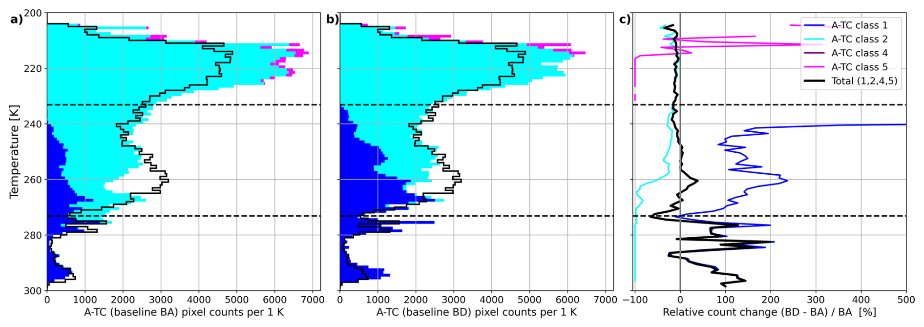
Figure 9 Stacked vertical distributions of A-TC cloud pixels in 1 K temperature bins (as in Fig. 6c) for the 12 EarthCARE underflight segments for which the BD products are available. (a) Cloud pixel shows distributions for baseline BA, panel (b) illustrates the corresponding distribution for baseline BD. (c) Relative change in cumulative cloud pixel counts between BD and BA, shown for all classes (black) combined and for individual cloud classes (colour coded). The cloud pixel count detected from WALES for the 12 flight is displayed as black line in panels (a) and (b). The horizontal dashed lines in panels (a)–(c) show the 273.15 K and the 236 K isotherms.

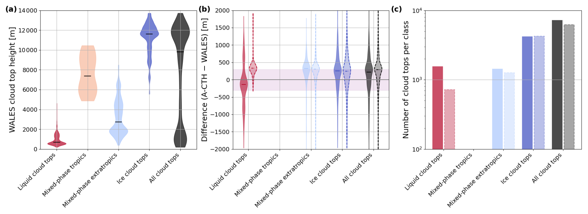
Figure 10 (a) Cloud top height distributions from WALES observations shown as violin plots for the same cloud regimes as defined in Fig. 8 (liquid, tropical and extratropical mixed-phase, ice clouds, and all cloud tops). (b) Differences in cloud top height relative to WALES (A-CTH − WALES) for the two A-CTH versions, with baseline BA shown as solid violins and baseline BD as dashed violins. (c) Corresponding number of cloud top observations per category for baseline BA (solid bars) and BD (dashed bars). All results are based on the full EarthCARE underflights of the 12 research flights. Note that violins in panels (b) and (c) are only displayed if a class includes more than 50 cloud top height counts.

Figure 10 presents WALES cloud top height distributions (a), corresponding differences to the two A-CTH versions (b), and counts per category (c) for the same temperature-based cloud classes as defined in Fig. 8, representing the same 12 research flights. The WALES cloud top height distributions (Fig. 10a) exhibit a similar overall structure to those shown in Fig. 8, with comparable altitude ranges and positions of the maxima across the different categories. However, the distribution of all cloud tops (black violin) reveals a pronounced bimodal structure, caused by the dominance of low-level and high-level clouds and an absence of mid-level clouds in this subset as opposed to the trimodal distribution shown in Fig. 8a. The missing mid-level peak is primarily associated with the limited occurrence of mixed-phase tropical clouds in the 12 analysed flights (see Fig. 10c). This is further reflected in the broad distribution of the mixed-phase tropical class, which results from the comparatively small number of detected cloud tops within this category. The distributions of cloud top height differences between WALES and the A-CTH versions (Fig. 10b) are comparable to Fig. 8. The baseline BA distributions (solid violins) are shifted toward positive values, indicating an overestimation of cloud top heights. In contrast, the baseline BD (dashed violins) cloud top differences are smaller in magnitude, particularly for the (extratropical) mixed-phase and ice cloud categories, suggesting a slight improvement in accuracy, although a systematic overestimation by BD remains evident. Due to the very low number of tropical mixed-phase clouds (< 50 cases) in this data subset, no comparison of cloud top differences is provided for this category. Notably, for the liquid cloud class, the BA distribution shows a trimodal structure, indicative of distinct regimes of over- and underestimation associated with misclassified very low cloud tops below 200 m, as discussed in Sect. 4.2. This trimodality is no longer present in the baseline BD distribution, as these misdetections low-level cloud tops have been effectively removed. As a result, the distribution for this class in baseline BD primarily reflects the remaining overestimation of cloud top heights. This change is also evident in Fig. 10c, showing a general reduction in cloud counts for the baseline BD across all categories, but most notably for the liquid cloud tops compared to the baseline BA.

5 Discussion

The scope of this study is the evaluation of selected cloud-related parameters from three ATLID Level 2 products: the “feature mask” of the A-FM product (van Zadelhoff et al., 2023), the “simple classification” of A-TC product (Irbah et al., 2023; Donovan et al., 2024) and the “cloud top height” from the A-CTH product (Wandinger et al., 2023), which provide essential parameters to characterize macrophysical properties of clouds. For this purpose, a comprehensive and independent multi-campaign airborne WALES BSR dataset is used to determine a cloud mask, providing the high spatiotemporal collocation required for robust validation (e.g. Hall, 2025; Groß et al., 2026). The corresponding multi-modal vertical distribution of cloud pixels for the multi-campaign dataset (Fig. 2) expresses the variety of clouds observed at low, mid, and high-levels and at different temperature ranges. The altitude of the maxima varies among the campaigns, with the highest altitude maxima observed during the tropical campaigns, while extratropical campaigns exhibit lower maxima consistent with reported seasonal and latitudinal variations (e.g., Stubenrauch et al., 2017). In general, the number of cloud detections in WALES decreases with decreasing altitude (i.e., as temperatures rise; see Fig. 6), which is primarily due to two characteristics of lidar measurements. First, optically dense ice clouds (e.g., anvil cirrus clouds) can attenuate the laser beam and thus prevent detection below the uppermost cloud layer. Second, clouds in the mixed phase and liquid phase are largely optically dense, so that the lidar primarily provides information about the cloud top rather than the entire vertical extent, which by nature lowers the amount of detected cloud pixels in these cloud types.

5.1 Validation of cloud features from the simple mask (A-TC) and the feature mask (A-FM)

The statistical analysis of the A-TC and A-FM products clearly shows that both products reproduce this multi-modal vertical cloud distribution observed by WALES, with individual maxima occurring at similar altitudes, and hence provide a notably realistic representation of the vertical cloud distribution given the early stage (baseline B) of these products. Nevertheless, several distinct differences between A-TC cloud targets and A-FM features and WALES cloud pixels could be identified. A slight underestimation of cloud features is found in the lowermost 2 km altitude in A-TC and A-FM, which may be related to the higher resolution of the WALES BSR data enabling detection of very small-scale clouds.

A-TC systematically overestimates the number of cloud pixels across nearly all altitudes, which is most pronounced when ice clouds dominate. This overestimation is primarily associated with the enhanced occurrence of thin-feature classes in A-FM (values 6 and 7), which are propagated into A-PRO and result in an increased frequency of ice cloud detections in A-TC (Irbah et al., 2023). Ice clouds in A-TC are furthermore typically horizontally larger and vertically deeper compared to the corresponding detected WALES cloud pixels. In addition, broken cirrus cloud formations in WALES appear less patchy in A-TC (typically as one coherent layer). However, these patchy structures are found in the Level 1 backscatter observations (not shown) and optical properties derived from it (e.g., the ATLID BSR in the Level 2 product A-EBD, see Figs. 3e and 4e) suggesting that the increase in ice cloud pixels arises in the Level 2 processing chain. Here, the patchy structure is also occasionally apparent in the three highest feature values (8–10) in the A-FM product. It has to be emphasized that A-TC liquid cloud pixels are strongly consistent with the WALES cloud mask with respect to the cloud lengths and their altitudes (Figs. 3, 4, 6). To further test the finding whether the observed A-TC ice cloud overestimation could be related to the chosen BSR threshold, a sensitivity analysis using variable BSR thresholds in the cloud detection supports that the overestimation in A-TC cloud pixels is not caused by selecting a too conservative BSR threshold in the WALES BSR observations (Appendix A).

Another feature observed in A-TC during mid- and high latitude flights is the occasional presence of stratospheric aerosol structures attached to ice cloud features, that are sharply separated at the tropopause. A-PRO uses the tropopause as a reference level to define backscatter thresholds for cloud detection (i.e., lower thresholds in the stratosphere, higher ones at the tropopause; see table 1 in Irbah et al., 2023). Cloud detection in A-PRO therefore also depends on the height of the tropopause. Although the tropopause is generally an important reference, it is not always clearly defined (e.g., it may exhibit discontinuities and large jumps in height near the jet stream, be poorly defined within the polar vortex, or be multi-valued; e.g., Schäfler et al., 2021; Krüger et al., 2022). Potentially incorrect tropopause heights can therefore influence feature detection in A-TC and A-CTH, and are likely responsible for the described sharp transition between ice clouds and “stratospheric aerosols” at the tropopause in the baseline BA (Fig. 4d). We emphasize that we were only able to diagnose this feature for extratropical frames, since the tropical tropopause lies far above the HALO flight level. We also want to stress that such misclassifications of ice cloud pixels as stratospheric aerosols are not observed in the more recent baseline BC (during the NAWDIC flights) and are much reduced for the midlatitude cases of the BA version (Fig. 9c). This is likely attributed through an improved tropopause determination as indicated in the data disclaimer (ESA, 2026a).

Furthermore, A-TC indicates enhanced classifications of ice cloud pixels embedded within aerosol layers, with detected ice clouds located at temperatures below and above the freezing level (273.15 K). This feature is particularly evident in tropical E-frames under conditions of elevated aerosol loading associated with Saharan dust outbreaks and appears most pronounced in the eastern Atlantic, near its source regions, but is also observed in the central and western Atlantic. Previous studies demonstrate that mineral dust can act as an efficient ice-nucleating particle, enabling heterogeneous ice formation within dust-laden air masses (e.g., Boose et al., 2016). However, this process typically requires temperatures well below −10 °C (Ansmann et al., 2005, 2008; Seifert et al., 2010). In contrast, the majority of ice cloud pixels identified here occur at temperatures above −10 °C and remain embedded within the Saharan dust layer, which suggests that these ice clouds may be misclassified in A-TC. Given that the optical properties of dense mineral dust and optically thin ice clouds can be similar (increased depolarization ratio, slightly increased lidar ratio; e.g., Groß et al., 2013) these ice cloud pixels are likely misclassified. A plausible explanation for this misclassification is an increased depolarization in the ATLID Level 1, or increased cross-polar channel noise reported by Groß et al. (2026). However, it is important to note that in the analysed subset of 12 cases for baseline BD, no ice cloud pixels are classified at temperatures above 273.15 K (Fig. 9b), indicating that this issue is expected to be no longer present in the upcoming Baseline C (as baseline BD is being considered a candidate for the next major baseline update). The disclaimer indicates that this improved ice cloud-liquid cloud discrimination is related to the use of temperature from improved X-MET product that was already implemented for Baseline BC (ESA, 2026a).

The A-FM product is designed to provide a probabilistic assessment of the presence of optically thin and optically thick features in the atmosphere, rather than making a strict distinction between clouds and aerosols. Consequently, a direct comparison with A-TC classifications is neither possible nor intended in this study. According to the A-FM feature definition (van Zadelhoff et al., 2023), both clouds and aerosols can appear as optically thin or optically thick features, which precludes a direct comparison with A-TC cloud pixels. Nevertheless, A-FM serves as input to the Level 2 processing chain, where it guides averaging strategies within the A-PRO processor. Hence, A-FM supports the generation of both single- and multi-sensor products and may therefore influence their overall quality. For this reason, an evaluation of A-FM classified features against WALES cloud observations is included in this study.

A strong agreement is shown between optically dense features in the A-FM product (values 8–10), representing thick clouds or dense aerosol layers, and cloud detections from WALES. In contrast, lower-ranked flags (values 6–7; Appendix B), which correspond to optically thin aerosol or cloud features, are widely present but are clearly not correlated to WALES cloud pixels. It is found that A-FM pixels classified as optically thick (values 8–10) also exhibit strong agreement with WALES detections in the ice cloud regime at high altitudes and are capable of reproducing their fragmented spatial structure (Figs. 3 and 4), which likely explains the high correlation observed with WALES (Fig. 6). At lower altitudes (or temperature > 273.15 K) interestingly, only the two highest A-FM values (9 and 10) accurately agree with cloud pixels detected by WALES, while inclusion of the value 8 leads to an overestimation of feature occurrence. This may be related to the presence of enhanced sea salt or Saharan dust frequently measured in this temperature regime, which could be assigned to value 8 in the A-FM product. Given the strong agreement between WALES-detected cloud pixels in the ice cloud regime and the A-FM feature mask (value 8–10), as well as the role of A-FM as input to the A-PRO algorithm (Donovan et al., 2024), it is speculated that a stricter use of these A-FM flags could improve the representation of ice clouds in the A-TC product.

In this study, the pre-operational baseline BD of the A-TC product is also analysed for 12 selected flights, providing an opportunity to assess potential improvements introduced in the upcoming baseline C. The evaluation of baseline BD reveals several changes in cloud pixel distribution compared to BA. Cloud pixels in cold regimes (< 250 K) decrease by 5 %–15 % in BD, although a general overestimation relative to WALES remains. This reduction is mainly caused by a partial reclassification of ice cloud pixels into aerosol, together with the successful removal of spurious stratospheric aerosol features (associated with ice clouds in Baseline BA) above 216 K (reduction by 100 %, see Fig. 9c), rather than by a reduction in ice cloud extent, which remains the main contributor to the ice cloud pixel overestimation. In addition, BD shows a shift in cloud phase partitioning toward increased liquid cloud occurrence and a more consistent separation between liquid and ice clouds. Ice cloud detections decrease across all temperature ranges, most strongly above 260 K, while the fraction of liquid clouds increases, particularly in the 290–296 K range where A-TC detects about twice as many clouds compared to WALES. An important finding is that the misclassification of ice clouds at temperatures above the freezing level is fully eliminated in BA.

5.2 Validation of the cloud top height product A-CTH

The statistical evaluation of the cloud top height product A-CTH, which is generated independently from A-FM and A-TC and derived directly from Level 1 backscatter signals, reveals several notable features regarding its accuracy and performance across different cloud regimes. The analysis of the full dataset indicates that A-CTH cloud top altitudes meets the overall target accuracy requirement of ±300 m (Wehr, 2006; Wandinger et al., 2023) for about 50 % of the cloud tops, whereas 80 % of the examined cloud top height differences are within ±500 m (Fig. 8). We find a strong indication for a systematic overestimation of cloud top heights by A-CTH is found, with cloud tops frequently exceeding WALES measurements on average by about 270 m. This positive bias may be related to too broadly chosen dilation of the wavelet employed in A-CTH for cloud top detection, which may favor higher detected cloud top altitudes.

The evaluation of cloud top differences for distinct clouds regimes shows a consistent overestimation (median between 260–300 m) in A-CTH for mixed-phase and ice clouds (Fig. 8), indicating that this bias is likely not related to the different temperatures and altitude of these cloud types. In contrast, the cloud top differences for low-level (liquid) clouds show a bimodal distribution, with distinct cluster indicating over- and underestimations of cloud tops. While the overestimation cluster (about 300 m) is consistent with findings in mixed-phase and ice-phase clouds, the underestimations are related to occasionally strikingly low cloud tops of about < 200 m in A-CTH. These very low clouds are found in tropical and extratropical frames predominantly over ocean but also occasionally above landmasses, and it is noted that they can occur in cases where no cloud could be detected by WALES, or indicated by A-TC/A-FM. These underestimations occur due to a known bug that occasionally led to misidentified surface return which should be resolved from baseline BB onwards (see: ESA, 2026b). It is found that such very low cloud top detections are no longer present in the Baseline BC and BD. The comparison of cloud top heights from A-CTH between baseline BA and BD further indicates a slight improvement in cloud top height accuracy in CA of the order of a few metres, and a small overall reduction in cloud pixel counts across the cloud classes.

Additionally, A-CTH cloud tops appear to have a strong agreement with the dense features (flag 9, 10) in A-FM, and particularly with the classified liquid cloud pixels in the A-TC product. It is shown that in cases of the above-mentioned misclassified ice cloud pixels inside aerosol layers, A-CTH typically does not identify a cloud top. On the other hand, for the likely mis-identified low-altitude cloud tops in A-CTH, the corresponding pixels in WALES and A-TC/A-FM (dense features) are located at similar altitudes. This underlines the advantage of the complementary use of the different products for cloud characterization in scientific applications. At this point, we emphasize the importance of airborne lidar observations for accurately determining cloud top heights in optically thick clouds, such as liquid-phase and mixed-phase clouds. For these cloud types, a direct observational perspective from above is required, as ground-based lidar systems are attenuated at the cloud base and cannot provide reliable information on cloud top height. Airborne (and spaceborne) lidar systems uniquely offer this capability, allowing for retrieval of cloud top altitudes and for the validation of A-CTH product.

5.3 Influence of representativeness (spatiotemporal matching of ATLID and WALES data)

A further important aspect that should be considered for a careful validation of ATLID cloud or aerosol products is the representativeness of the collocated reference observations (Floutsi et al., 2026). Clouds are dynamic atmospheric features, evolving vertically (e.g., in convection) and are advected horizontally by the wind. This introduces an intrinsic uncertainty for a statistical validation, as cloud fields may drift into or out of the observation scene (i.e., the satellite ground track). As a result, cloud features may be detected by one instrument but missed by the other, even in the absence of retrieval uncertainties in the ATLID or WALES products. It is impossible to assess representativeness profile by profile for the applied large airborne data set. In a statistical sense, representativeness is expected to improve with increasing spatial and temporal collocation; however, restricting the comparison to a narrowly defined region around the underpass – where ATLID and WALES measurements are best collocated – would substantially reduce the number of detected cloud samples. This reduction makes the statistical assessment prone to outliers, potentially skewing the results. To account for these effects, two complementary validation approaches are considered in this study: (1) A statistical validation based on all observations acquired for the full length of each satellite underpass segment since mismatches due to cloud motion may cancel out when using the maximum available number of collocated data. (2) A statistical comparison using a subset of data collected within 10 min. of the underpass assuming the better spatial/temporal collocation would improve representativeness.

For the selected subset the number of detected cloud pixels decreases expectedly at all altitudes reflecting the stricter collocation criteria; however, the shape of the vertical distribution of both WALES cloud pixels and A-TC/A-FM features remains robust (see Appendix C, D). Hence, the key findings reported in Sect. 5.1 such as the overestimation of (ice) cloud pixels in A-TC, the classified stratospheric aerosol features attached to ice cloud layers separated by a tropopause, and the presence of ice cloud pixels (particularly in Saharan dust layers) are also confirmed only the subset of the data with higher representativeness. Similarly, for A-CTH, the documented cloud top height overestimation is a persistent feature, even when the analysis is limited to data within the 10 min. matching window. In general, representativeness should be carefully considered in any validation study, in particular those targeting highly dynamic atmospheric phenomena such as clouds. This is particularly important for case studies (in our case individual flight statistic), whereas the use of large datasets may allow for a partial compensation of representativeness-related uncertainties through statistical averaging.

6 Summary

The EarthCARE satellite mission is designed to advance our understanding of the interactions between clouds, aerosols, and radiation in the Earth's climate system (Illingworth et al., 2015; Wehr et al., 2023), with the ATLID instrument playing a central role to these goals providing data to retrieve both cloud and aerosol related products (Eisinger et al., 2024). Validation of these products is a crucial prerequisite for their scientific application (e.g., Amiridis et al., 2025; Hall, 2025; Baars et al., 2026; Kubota et al., 2026). This study presents a validation of cloud properties of three selected ATLID Level 2 single-sensor products (A-TC, A-FM, and A-CTH) with a comprehensive multi-campaign dataset of airborne WALES HSRL BSR measurements. The observations cover a broad range of cloud conditions (i.e., temperature regimes) in the tropics and extratropics. The high spatiotemporal coordination of the satellite and airborne platforms provides a robust and independent validation framework. This validation study focuses on two main objectives: (1) assessing whether the A-TC “simple classification” and A-FM “feature mask” realistically represent the observed vertical cloud distribution, and (2) evaluating whether A-CTH cloud top heights achieves the 300 m accuracy target across different cloud regimes. A summary of these objectives is provided below.

The vertical distribution of clouds observed with WALES is well captured by both A-TC and A-FM products. In particular, A-FM (values 8, 9, 10) shows strong agreement with airborne observations in representing cloud structures, especially for ice clouds, where it realistically resolves patchy structures as well as vertical and horizontal extent. Cloud top heights from A-CTH are, on average, already close to the mission's accuracy requirement (Wandinger et al., 2023). However, several systematic discrepancies have been identified. The A-TC product tends to overestimate ice cloud occurrence, likely due to spreading effect caused in the retrieval that act to fill gaps between broken cloud structures and increase cloud size. In contrast, liquid cloud fractions show a very good agreement with the airborne observations. Additional documented issues include the misclassification of stratospheric aerosol near the tropopause and the appearance of ice cloud pixels at temperatures above freezing level within dense aerosol layers. The A-CTH product exhibits positive cloud top height bias, i.e., overestimates cloud tops by almost 300 m which is consistently found for different temperature regimes, including ice clouds, mixed-phase and liquid clouds. Furthermore, occurrences of unexpectedly low cloud tops (< 200 m altitude) indicate potential issues in the retrieval with surface assignment especially over the ocean. It should be noted that the results presented above primarily refer to baseline BA. An analysis of 5 NAWDIC flights (baseline BC) and the subset of 12 research flights with the BD baseline highlights some improvements expected in the upcoming baseline C, which include a removal of unrealistically low cloud tops detections in A-CTH, as well as a more coherent representation of liquid and ice clouds and an improved classification of cloud pixels above freezing level in A-TC, supported by an improved tropopause in the X-MET product.

The key message of this study is that cloud parameters all validated ATLID Level 2 products (A-FM, A-TC, A-CTH) demonstrate remarkably good consistency with the cloud mask determined from the independent WALES data set, highlighting their readiness for scientific applications. Users should be aware that these products are still at an early stage of development and may therefore still be subject to residual uncertainties. Careful quality assessment of the applied ATLID Level 2 data is therefore recommended. Continued evaluation of future processing baselines, validation of ATLID aerosol products, and the inclusion of JAXA products is encouraged to support further improvements in retrieval algorithms and to fully realize the scientific potential of ATLID observations.

Appendix A: Cloud pixel sensitivity to the chosen BSR threshold

The algorithm used to derive cloud pixels from WALES BSR is described in Sect. 2, where the selected BSR threshold for the cloud–no-cloud decision is justified based on previous studies (e.g., Groß et al., 2014; Urbanek et al., 2018; Gutleben et al., 2019; Dekoutsidis et al., 2024). To assess the sensitivity of cloud detection to this threshold, the BSR value is varied while keeping temperature constant. As expected, the number of detected cloud pixels increases when lowering the threshold to 1.2 at all altitudes, particularly in the lower troposphere, where aerosol contributions (e.g., sea salt and mineral dust) are more frequent. Conversely, more conservative (higher) thresholds result in fewer detections. Even for the relatively low threshold of 1.2, the maximum number of detected cloud pixels (around 11 km altitude) remains below that of A-TC. This suggests that the cloud overestimation observed in A-TC is unlikely to be solely explained by the choice of the WALES BSR threshold.

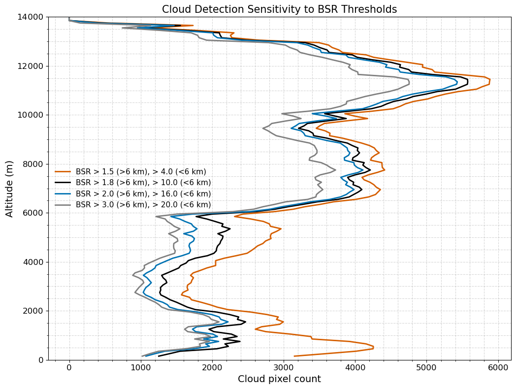
Figure A1 Cloud pixel counts from WALES BSR as detected for variable BSR and temperature thresholds.

Appendix B

Section 5.3 discusses the influence of potential spatial and temporal mismatches on the findings of this work. To support this, we provide four figures illustrating the validity of the results. These show the cloud pixel distributions from the A-TC and A-FM products (as in the main text) but restricted to a 10 min window around the underpass. Figure B1 additionally includes the classified thin features from A-FM, which often represent aerosols rather than clouds and are therefore excluded from the main comparison. Appendices B1 and C1 show A-TC and A-FM for periods of highest expected spatiotemporal collocation. The main finding – an overestimation of cloud pixels in A-TC – remains unchanged when restricting the analysis to this higher-collocation subset, indicating that the results are not significantly affected by spatial or temporal mismatch.

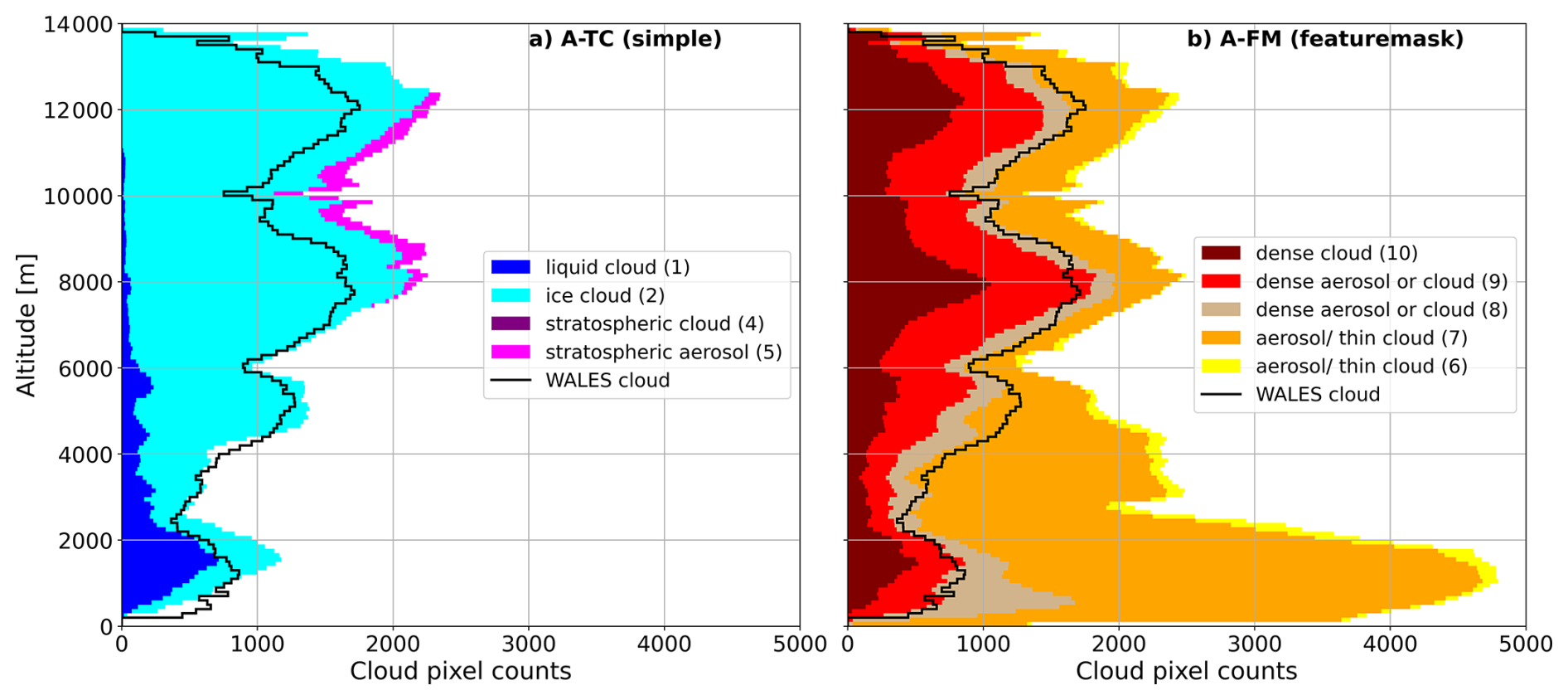
Figure B1 Same as Fig. 6a, b but inclusion of thin features in A-FM (values 6, 7). Shown are data within ±10 min; 138 km centred around the EarthCARE underpass. Note that the x-axis are changed compared to Fig. 6.

Appendix C

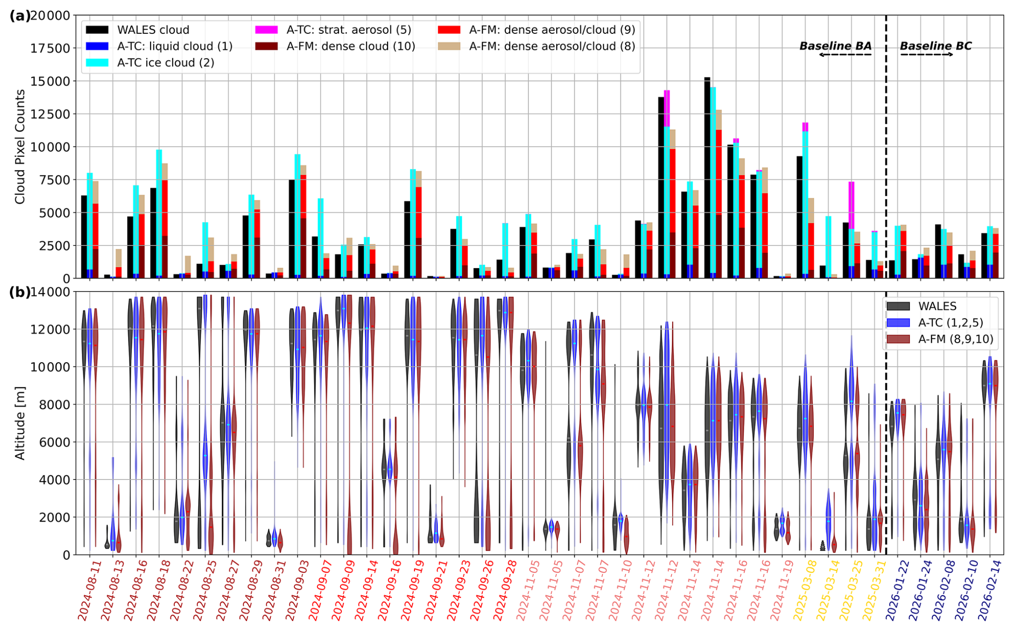
Figure C1 Same as Fig. 5, for data within ±10 min; 138 km centred around the EarthCARE underpass.

Appendix D

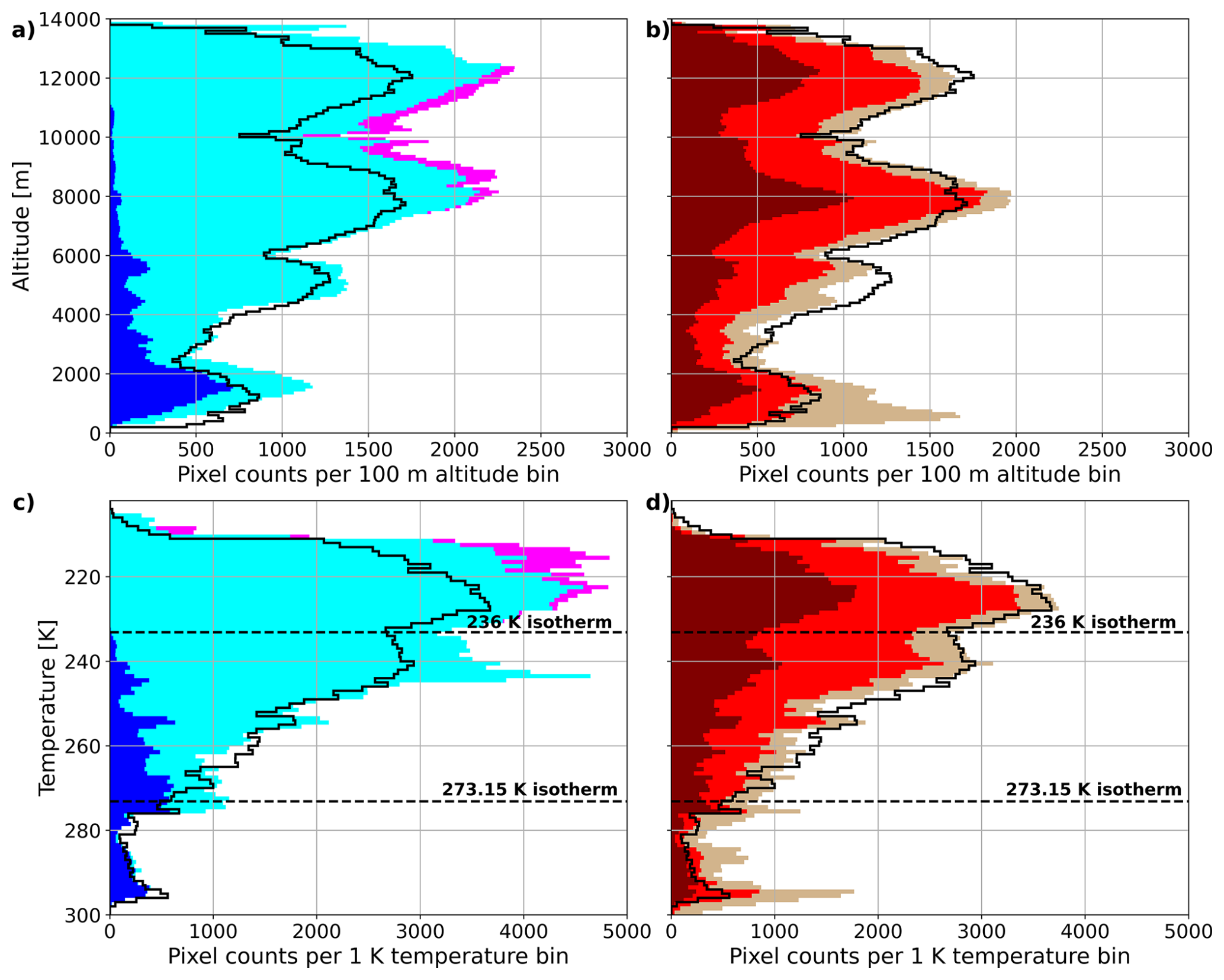
Figure D1 Same as Fig. 6c, d, but focus on observations within ±138 km/10 min, with the same coloring of the different flags of A-FM and A-TC. The similarity of the distributions compared to Fig. 6 underlines the strong consistency between cloud pixels of the full dataset and the segments close to the underpass (i.e., of higher expected representativeness).