Estimating near-surface specific humidity over convective oceanic regions from cloud base height observations

The surface moisture flux is a large term in the surface energy balance and difficult to estimate remotely. The main difficulty for its remote estimation is a poor ability to measure near-surface humidity. Current methods to retrieve near-surface specific humidity approach the problem statistically and have errors of approximately 1 g kg⁻¹ even in global, annual averages. Using extensive measurements from the EUREC⁴A field campaign (ElUcidating the RolE of Cloud-Circulation Coupling in Climate), we demonstrate that remote sensing measurements of cloud base height can provide useful estimates of near-surface humidity over convective oceanic regions where optically-thick clouds do not prevent lidar sampling. First applying the method to 171 coincident radiosonde and ceilometer pairings collected from a research vessel from 18 January to 14 February 2020 yields skillful predictions of near-surface specific humidity regarding the mean (mean bias 0.43 g kg⁻¹ compared to observed) and its variability (r=0.76). We then apply this method using an airborne lidar to estimate cloud base height from above. In two representative case studies, we find similar skill in the predicted humidity, with low mean biases (0.04 and −0.06 g kg⁻¹ compared to observed) with substantial variability captured (r=0.61 and r=0.57, respectively). Besides estimates of cloud base height, we highlight two main error sources: (i) the relative humidity lapse rate below cloud base and (ii) the temperature difference between the sea surface and near-surface air, which would need to be calibrated if using this method to develop an operational product to estimate the near-surface specific humidity from downward-looking spaceborne lidar. This proof of concept raises the potential for application over convective oceanic regions where lidar sampling of cloud base is possible. This method could provide a physics-based augmentation to existing, more empirical approaches and therefore provide an additional observational constraint on the surface energy budget.

1 Introduction

The surface energy balance is a fundamental property of the climate system. How it is partitioned among its different components, and how it varies in space and time tempers the behavior of the atmosphere above, and the land or water below (e.g., Hartmann, 2015). Among its varied components, the main balance is between moisture fluxes, extracting energy from the surface through evaporation, and the absorption of energy from the sun. Sensible energy transfers, and net radiant energy fluxes in the thermal infrared also combine to cool the surface, but on average only half as strongly as the evaporation of water which maintains the flux of moisture to the atmosphere (e.g., Hartmann, 2015). In addition to providing an energetic link between the surface and the atmosphere, the moisture flux links the water and the energy cycles (e.g., Jackson et al., 2009; Kubota and Hihara,, 2008; Fajber et al., 2023). Despite their importance, the evaporative (or moisture) fluxes are difficult to measure, and they are both one of the largest, and most uncertain terms in the surface energy balance (e.g., Liman et al., 2018; Clayson et al., 2019). An improved ability to quantify evaporative fluxes is therefore essential for observation-based studies of the water and energy cycles, and the dynamics of weather systems and circulations that they fuel.

These fluxes can be reasonably well estimated from the covariance of anomalies in moisture, q^′, and vertical air motions, w^′, i.e., as $\mathit{\rho }{\mathrm{\ell }}_{\mathrm{v}}\stackrel{\mathrm{‾}}{w^{\prime }{q}^{\prime }},$ with ρ the density and ℓ_v the vaporization enthalpy. Surface layer similarity provides a mean field theory for the evaporative flux, which is encapsulated by the bulk aerodynamic formula (e.g., Fairall et al., 1996b, 2003; Edson et al., 2013), taking the form,

$$\begin{array}{}\text{(1)}& \stackrel{\mathrm{‾}}{w^{\prime }{q}^{\prime }}=C\left|U\right|\mathrm{\Delta }q,\text{where}\mathrm{\Delta }q\equiv q_{\mathrm{s}}-q_{\mathrm{a}}\end{array}$$

so that the evaporative flux can be directly related to the difference, Δq, in the specific humidity deficit of the air, q_a, as compared to the surface, q_s, and the near-surface wind speed, $\left|U\right|$, with C being an exchange coefficient. The value of C depends on surface properties and atmospheric stability (often expressed using Monin–Obukhov similarity and the stability parameter $z/L$), and has been characterized by decades of observations and theory (Fairall et al., 1996b, 2003; Edson et al., 2013). We refer to COARE as a representative bulk algorithm but note that different bulk formulations and transfer-coefficient parameterizations can yield differing latent heat flux estimates for identical bulk inputs, particularly under very low- and very high-wind conditions. Thus, uncertainties in q_a influence flux estimates directly through Δq and indirectly through stability-dependent transfer coefficients. The surface moisture fluxes can therefore be reasonably well determined given knowledge of the specific humidity of the near-surface air, q_a, the saturation specific humidity at the surface temperature and pressure, q_s, as well as the near-surface winds, $\left|U\right|$.

Following the bulk aerodynamic formulation of surface fluxes, we assume that the water vapor pressure at the ocean surface is at saturation, so that the surface specific humidity q_s equals the saturation specific humidity $q_{*}(T_{\mathrm{s}},P_{\mathrm{s}})$. This approximation in bulk theory reflects the near-equilibrium condition at the air–sea interface and is a standard assumption in flux parameterizations, sometimes with a 0.98 correction for typical salinity (e.g., Fairall et al., 1996b, 2003). Satellite remote sensing can provide reasonable estimates of T_s, which given P_s determines q_* and hence q_s. Likewise a variety of measurements provide increasingly accurate estimates of surface wind speeds (e.g., Ricciardulli and Manaster, 2021). The main limitation in estimating evaporative fluxes over the ocean is therefore the measurement of the near-surface specific humidity of the air, q_a, a quantity for which there is no real proxy. As a result, satellite-based climatologies of evaporative fluxes over the ocean depend on q_a correlating with other quantities that can be remotely sensed, so that it (or the evaporative flux as a whole) can be inferred statistically. Various approaches to this problem are described in Gentemann et al. (2020). These include retrievals from passive microwave measurements, such as the Hamburg Ocean Atmosphere Parameters and Fluxes from Satellite (HOAPS4) (Liman et al., 2018; Andersson et al., 2010) and SeaFlux CDR (Clayson and Brown, 2016), as well as approaches that combine reanalysis and passive microwave data, such as IFREMER4 (Bentamy et al., 2013, 2017a) and J-OFURO3 (Tomita et al., 2019). Liman et al. (2018), for instance, compared HOAPS climatology with in situ buoy and ship measurements and found retrieval uncertainties in latent heat flux of 15 W m⁻², with a global-mean error of 25 W m⁻². Errors were found to be particularly large over the subtropical oceans, where evaporative fluxes are large in magnitude, with an average of 37 W m⁻² in random instantaneous retrieval errors (Liman et al., 2018).

A number of studies have confirmed that the most uncertain term in Eq. (1) is q_a (e.g., Bourras, 2006; Tomita and Kubota, 2006; Jackson et al., 2009; Bentamy et al., 2017b; Roberts et al., 2019; Robertson et al., 2020). Liman et al. (2018) estimated that contributions from q_a contribute approximately 60 % to overall uncertainty in the evaporative flux, whereas uncertainties from the wind speed contribute about 25 %.

Given this uncertainty, our goal is to develop a method to estimate q_a over convective oceanic regions. To this end, we exploit the physical connection between cloud base height h and near-surface relative humidity W_a: in a convective, well-mixed subcloud layer the cloud base forms near the lifting condensation level (LCL) and thus the height at which it forms depends primarily on near-surface T and q.

Our method takes advantage of the fact that a convective cloud-topped boundary layer is ubiquitous over the world oceans (Fig. 1). We demonstrate this ubiquity by analyzing daily ERA5 surface fluxes from the year 2020 to compute the climatological frequency of positive surface buoyancy flux, B₀, representing the annual frequency of convectively unstable surface conditions. The resulting “buoyancy-favorability” map (Fig. 1) shows that near-surface convective instability prevails over most tropical and subtropical oceans, with ocean-only mean frequencies of 85 % globally and 99 % between 30° S and 30° N.

Building on this link, we test the idea that W_a (and hence q_a) can be inferred from h and a small set of parameters, as a basis for a possible retrieval. To this end, we summarize notation and data (Sect. 2); we then derive the relationship between h, W_a, and $\mathrm{\Delta }q\equiv q_{\mathrm{s}}-q_{\mathrm{a}}$ and quantify sources of uncertainty (Sect. 3). Using coincident ceilometer–radiosonde and lidar–dropsonde measurements from EUREC⁴A, we validate the h–W_a linkage from surface and airborne platforms (Sect. 4.1, 4.2). We estimate the two near-surface control parameters, $\mathrm{d}W/\mathrm{d}z$ and Δ_aT, from observations (Sect. 4.3) and evaluate retrieval skill in q_a (Sect. 4.4). Finally, we discuss scope, caveats, and practical use, and conclude (Sects. 5, 6).

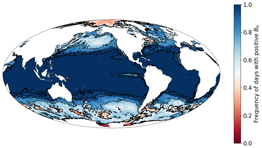
Figure 1 Frequency of days with positive surface buoyancy flux, B₀, during 2020, computed from daily ERA5 reanalysis data of sensible and latent heat fluxes, as well as the 2 m air temperature. The shading indicates the fraction of days for which the surface buoyancy flux is positive (upward). Positive values represent convectively unstable surface conditions. Values approach unity over most tropical and subtropical ocean regions, indicating nearly continuous convective instability. Values below 50 % frequency are shown in red. Over the global oceans, the area-weighted mean frequency is approximately 85 %, while in the tropical band (30° S–30° N) it reaches 99 %. Black contours denote frequencies of 0.50, 0.75, 0.90, 0.95, and 0.99.

2 Notation and data

Throughout, for notation, the subscript s denotes surface quantities and the subscript a denotes near-surface atmospheric quantities evaluated at the reference height z_a=40 m. This height corresponds to the lowest reliable sonde level and is close to the R/V Meteor air-temperature measurements at 28.3 m used in this study. The ocean surface temperature T_s is the skin temperature. Near-surface atmospheric variables carry the a subscript; for example, q_a, T_a, and W_a refer to conditions at z_a. Air pressure is denoted by P and vapor pressure by e, with e_* denoting the saturation value for a plane of pure water. Hence, because the surface is water (albeit wavy and not pure), $e_{\mathrm{s}}\approx e_{*}\left(T_{\mathrm{s}}\right)$. To make it easier to manipulate in equations, for which abbreviations make poor symbols, we use the symbol W to denote relative humidity.

Regarding data, we employ coincident sounding and lidar data from a variety of ground-based and airborne observing platforms deployed as part of the EUREC⁴A field campaign (ElUcidating the RolE of Cloud-Circulation Coupling in Climate), which took place in January and February 2020 in the trade-wind zone east of Barbados (Bony et al., 2017; Stevens et al., 2021). During EUREC⁴A the German High Altitude and Long Range Research Aircraft (HALO) launched 810 dropsondes between 22 January and 15 February 2020 (George et al., 2021) (see the EUREC⁴A data paper for HALO by Konow et al., 2021). These dropsondes yield vertical profiles of pressure, temperature, and relative humidity with a manufacturer-stated accuracy of 0.4 hPa, 0.1 °C, and 2 %, respectively (Vaisala, 2020). One unique aspect of EUREC⁴A is the sampling strategy that provides aggregated, statistical estimates of a larger-scale signal, compared to individual point-wise measurements. During EUREC⁴A, dropsonde measurements were distributed along a fixed flight pattern, the “EUREC⁴A circle” – a circular flight pattern with an approximately 220 km diameter, centered at 13.3° N, 57.7° W, at 9.5 km altitude. Following Bony et al. (2017); Stevens et al. (2021), one circle-mean refers to the mean of typically 12 dropsondes launched over one hour along the EUREC⁴A circle (due to operator and instrument errors, on some circles fewer sondes were launched, but never fewer than seven). A circling-mean is defined as the mean of three consecutive circle-means (or in two cases, two circle-means), corresponding to 30–36 consecutive soundings aggregated over 210 min.

Also from HALO, atmospheric backscatter and water vapor DIfferential Absorption Lidar (DIAL) profiles were recorded using the airborne demonstrator for the WAter vapor Lidar Experiment in Space (WALES) (Wirth et al., 2009) onboard HALO. Due to its high horizontal and vertical resolution, airborne lidar data is amenable to studying small-scale clouds, such as in trade cumulus regions. Here we evaluate the lidar data at the highest possible resolution, e.g., the backscatter ratio and aerosol depolarization data are analyzed at 0.2 s time resolution and 7.5 m vertical resolution. For the analyzed flights, the altitude was nearly constant (∼ 10.4 km) and the aircraft speed was about 210 m s⁻¹, resulting in consistent horizontal spatial resolution of ∼ 42 m. Only data at a wavelength of 532 nm are used. The backscatter profiles are extinction corrected using the High Spectral Resolution Lidar (HSRL) method (Esselborn et al., 2008). All data are regridded to a constant altitude scale over the EGM96 geoid.

During the same period, radiosondes were launched as part of the campaign from the Barbados Cloud Observatory (BCO, Stevens et al., 2016) and the research vessel, R/V Meteor (Stephan et al., 2021), from 16 January to 1 March 2020. Ceilometer measurements of cloud base height were made from 18 January to 14 February 2020 from the same platforms. At the BCO the ceilometer is an OTT CHM 15k pulsed laser cloud height detector at 1064 nm used to detect cloud base height and lifting condensation level; at the R/V Meteor, the ceilometer is a Jenoptik system measuring vertical profiles of attenuated backscatter at 1064 nm to infer cloud base as a function of altitude and aerosol (Stevens et al., 2021).

3 Theory and parameter sensitivities for cloud base height as a proxy for near-surface humidity

Before quantifying empirical relationships between cloud base height, h, and near-surface relative humidity (W_a), we outline the theoretical basis linking both quantities. In a well-mixed and unsaturated subcloud layer, the specific humidity is nearly constant while temperature follows a dry-adiabatic profile. Relative humidity is defined as

$$\begin{array}{}\text{(2)}& W={\displaystyle \frac{e}{e_{*}\left(T\right)}}=q{\displaystyle \frac{R_{\mathrm{v}}}{R}}{\displaystyle \frac{P}{e_{*}\left(T\right)}},\end{array}$$

where $R=(\mathrm{1}-q)R_{\mathrm{d}}+q{R}_{\mathrm{v}}$ is the gas constant of an ideal mixture of “dry-air” and water vapor, e_*(T) is the saturation vapor pressure, and q the specific humidity.

For an adiabatic process for which pressure varies hydrostatically, $\mathrm{d}T/\mathrm{d}z=-g/c_p$, and negligible vertical humidity gradients ($\mathrm{d}q/\mathrm{d}z\approx \mathrm{0}$), the vertical gradient of W simplifies to

$$\begin{array}{}\text{(3)}& {\displaystyle \frac{\mathrm{d}W}{\mathrm{d}z}}={\displaystyle \frac{g}{T}}\left({\displaystyle \frac{{\mathrm{\ell }}_{\mathrm{v}}}{c_p{R}_{\mathrm{v}}T}}-{\displaystyle \frac{\mathrm{1}}{R}}\right)W,\end{array}$$

which gives the adiabatic rate of increase of relative humidity with height. Averaging across a well-mixed boundary layer with a depth of 600 m, $q=\mathrm{15}\mathrm{g}{\mathrm{kg}}^{-\mathrm{1}}$ and T varying dry-adiabatically about a mid-layer (300 m) mean value of 296.41 K – values derived from the Meteor and BCO radiosondes – yields a boundary layer mean value of $\frac{\mathrm{d}W}{\mathrm{d}z}=\mathrm{4.0}\mathrm{\%}{\mathrm{hm}}^{-\mathrm{1}}$ (referring to percent per hectometer, or 100 m).

Our analytical framework is closely related to earlier work connecting near-surface thermodynamic properties to the lifting condensation level. Lawrence (2005) provided a simple linear approximation relating the dewpoint depression to relative humidity, showing that $W\approx \mathrm{1}-(T-T_{\mathrm{d}})/A$ with A≈4.3 K near typical surface conditions; inverting this for a well-mixed subcloud layer yields an LCL height proportional to the dewpoint depression, consistent with the classical 125 m K⁻¹ rule. Romps (2017) derived an exact, implicit expression for the LCL temperature and pressure by conserving entropy and total water along a dry adiabat, obtaining an analytical result valid over a wide range of conditions. Our approach differs in emphasis, in that rather than computing the LCL from surface (T,q), we invert the relationship – given a remotely sensed cloud base height h, we recover W_a and hence q_a.

In reality, the subcloud layer departs slightly from adiabaticity due to entrainment of drier air from above and the partial compensation of temperature and moisture tendencies by turbulent mixing (Wyngaard and Brost, 1984), or due to rainfall and cold pools. Allowing weak vertical gradients in both T and q, the more general form of the relative-humidity lapse rate is

$$\begin{array}{}\text{(4)}& {\displaystyle \frac{\mathrm{d}W}{\mathrm{d}z}}=\left[\left({\displaystyle \frac{\mathrm{1}}{q}}-{\displaystyle \frac{R_{\mathrm{v}}-R_{\mathrm{d}}}{R}}\right){\displaystyle \frac{\mathrm{d}q}{\mathrm{d}z}}-{\displaystyle \frac{g}{RT}}-{\displaystyle \frac{{\mathrm{\ell }}_{\mathrm{v}}}{R_{\mathrm{v}}{T}^{\mathrm{2}}}}{\displaystyle \frac{\mathrm{d}T}{\mathrm{d}z}}\right]W,\end{array}$$

which reduces to Eq. (3) when $\mathrm{d}q/\mathrm{d}z=\mathrm{0}$ and $\mathrm{d}T/\mathrm{d}z=-g/c_p$.

Using representative trade-wind conditions from Albright et al. (2022), $\mathrm{d}q/\mathrm{d}z\approx -\mathrm{1}\mathrm{g}{\mathrm{kg}}^{-\mathrm{1}}{\mathrm{km}}^{-\mathrm{1}}$ and $\mathrm{d}T/\mathrm{d}z\approx -\mathrm{9.4}\mathrm{K}{\mathrm{km}}^{-\mathrm{1}}$, together with T=296.4 K and $q=\mathrm{15}\mathrm{g}{\mathrm{kg}}^{-\mathrm{1}}$, Eq. (4) gives $\left(\frac{\mathrm{1}}{W}\right)\frac{\mathrm{d}W}{\mathrm{d}z}\approx \mathrm{4.0}\times {\mathrm{10}}^{-\mathrm{4}}{\mathrm{m}}^{-\mathrm{1}}$, corresponding to $\frac{\mathrm{d}W}{\mathrm{d}z}\approx \mathrm{3.6}\mathrm{\%}{\mathrm{hm}}^{-\mathrm{1}}$ for W≃0.9. This non–well-mixed estimate is about 10 % smaller than the adiabatic value, with most of the reduction arising from the moisture-dilution term $(\frac{\mathrm{1}}{q}-\frac{R_{\mathrm{v}}-R_{\mathrm{d}}}{R})\frac{\mathrm{d}q}{\mathrm{d}z}$.

3.1 From relative to specific humidity

Given a cloud base at height h, where W=100 %, the relative humidity at a reference height z_a below cloud base can be approximated as

$$\begin{array}{}\text{(5)}& W_{\mathrm{a}}\approx \mathrm{1}-(h-z_{\mathrm{a}}){\displaystyle \frac{\mathrm{d}W}{\mathrm{d}z}}.\end{array}$$

From Eq. (2), the near-surface specific humidity deficit, $\mathrm{\Delta }q=q_{\mathrm{s}}-q_{\mathrm{a}}$, may then be written as

$$\begin{array}{}\text{(6)}& \mathrm{\Delta }q=q_{\mathrm{s}}\left\{\mathrm{1}-W_{\mathrm{a}}\left[{\displaystyle \frac{e_{*}\left(T_{\mathrm{a}}\right)}{e_{*}\left(T_{\mathrm{s}}\right)}}\right]{\displaystyle \frac{P_{\mathrm{s}}-[\mathrm{1}-R_{\mathrm{d}}/R_{\mathrm{v}}]e_{*}\left(T_{\mathrm{s}}\right)}{P_{\mathrm{a}}-[\mathrm{1}-R_{\mathrm{d}}/R_{\mathrm{v}}]W_{\mathrm{a}}{e}_{*}\left(T_{\mathrm{a}}\right)}}\right\}.\end{array}$$

Linearizing e_*(T) about T_s using the Clausius–Clapeyron relation,

$$\begin{array}{}\text{(7)}& e_{*}\left(T_{\mathrm{a}}\right)\approx e_{*}\left(T_{\mathrm{s}}\right)[\mathrm{1}-\mathit{\chi }{\mathrm{\Delta }}_{\mathrm{a}}T],\mathit{\chi }={\displaystyle \frac{{\mathrm{\ell }}_{\mathrm{v}}}{R_{\mathrm{v}}{T}_{\mathrm{s}}^{\mathrm{2}}}}\approx \mathrm{1}/\mathrm{16}{\mathrm{K}}^{-\mathrm{1}},\end{array}$$

and neglecting small pressure effects simplifies Eq. (6) to

$$\begin{array}{}\text{(8)}& \mathrm{\Delta }q\approx q_{\mathrm{s}}\left[\mathrm{1}-W_{\mathrm{a}}+\mathit{\chi }{\mathrm{\Delta }}_{\mathrm{a}}T{W}_{\mathrm{a}}\right],\end{array}$$

where ${\mathrm{\Delta }}_{\mathrm{a}}T=T_{\mathrm{s}}-T_{\mathrm{a}}$ is the sea–air temperature difference. Substituting Eq. (5) links Δq explicitly to h, the vertical gradient $\mathrm{d}W/\mathrm{d}z$, and Δ_aT.

The corresponding fractional uncertainty in Δq from errors in h and Δ_aT (first-order propagation) is

$$\begin{array}{}\text{(9)}& {\mathit{\epsilon }}_q\approx W_{\mathrm{a}}{\mathit{\epsilon }}_h+{\displaystyle \frac{\mathit{\chi }{\mathrm{\Delta }}_{\mathrm{a}}T{W}_{\mathrm{a}}}{\mathrm{1}-(\mathrm{1}-\mathit{\chi }{\mathrm{\Delta }}_{\mathrm{a}}T)W_{\mathrm{a}}}}({\mathit{\epsilon }}_h+{\mathit{\epsilon }}_T),\end{array}$$

where ${\mathit{\epsilon }}_h\equiv \mathit{\delta }\left[h\right(\mathrm{d}W/\mathrm{d}z\left)\right]/\left[h\right(\mathrm{d}W/\mathrm{d}z\left)\right]$ and ${\mathit{\epsilon }}_T\equiv \mathit{\delta }\left({\mathrm{\Delta }}_{\mathrm{a}}T\right)/{\mathrm{\Delta }}_{\mathrm{a}}T$ are fractional errors, and W_a is used as a fraction. For typical values W_a=0.90, Δ_aT=1.0 K, and $\mathit{\chi }\approx \mathrm{1}/\mathrm{16}{\mathrm{K}}^{-\mathrm{1}}$,

$${\mathit{\epsilon }}_q\approx \mathrm{1.26}{\mathit{\epsilon }}_h+\mathrm{0.36}{\mathit{\epsilon }}_T.$$

This analysis reinforces Eq. (8): the dominant source of uncertainty in Δq is the estimate of the product $h(\mathrm{d}W/\mathrm{d}z)$. Errors in the air–sea temperature contrast, Δ_aT, also affect the surface energy budget through the sensible heat flux and through the inferred humidity deficit. Their relative importance depends on the Bowen ratio, B, defined as the ratio of sensible to latent heat flux. For typical oceanic conditions, B≈0.1 (Oliver, 2005), indicating that latent heat flux generally dominates over sensible heat flux at the ocean surface. In this regime, uncertainties in Δ_aT can affect both the inferred humidity deficit and the sensible heat flux, but they remain less important than uncertainties in $h(\mathrm{d}W/\mathrm{d}z)$ for estimating Δq.

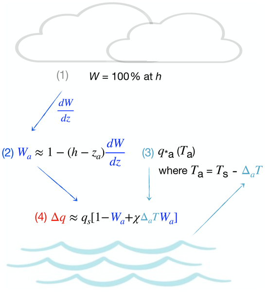
Figure 2 summarizes these relationships schematically, showing how h, $\mathrm{d}W/\mathrm{d}z$, and Δ_aT combine to determine the near-surface specific humidity deficit Δq.

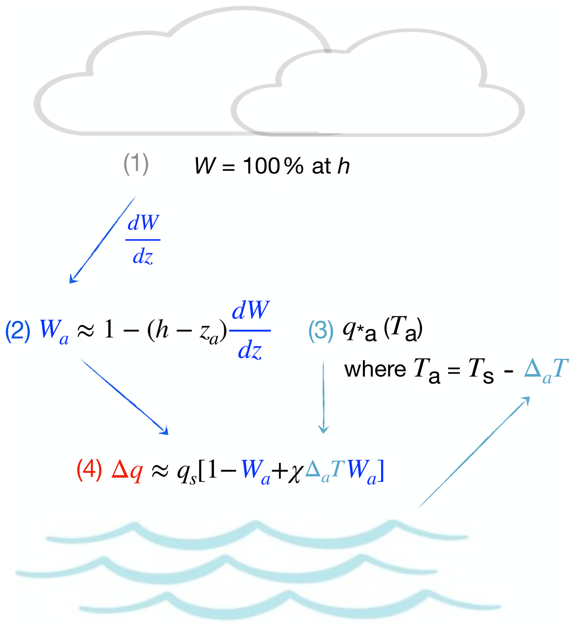
Figure 2 Schematic overview of the methodology highlighting the main error sources: (1) estimating cloud base height, h, at which W=100 % is assumed and then extrapolating W downward to z_a using (2) a fixed relative humidity lapse rate $\frac{\mathrm{d}W}{\mathrm{d}z}$, which is then converted to q_a as described in the text with a fixed ${\mathrm{\Delta }}_{\mathrm{a}}T=\mathrm{1.0}\mathrm{K}.$

4 Results

4.1 Ground-Based Validation

For the ground-based validation, we use W from radiosondes and cloud base height distributions that are derived from ceilometer measurements during 60 min windows centered on the radiosonde launch time. From the resulting distribution of ceilometer cloud detections, we associate h with the first and major peak of the distribution calculated from a Gaussian kernel density estimate, similar to the method employed in Albright et al. (2022) and Vogel et al. (2022). There is a strong correlation between h and the 10th percentile (r=0.94) or other low quantiles. Associating cloud base with the main peak of the distribution (or low quantiles) accounts for the expectation that ceilometer based cloud detections are skewed to more elevated values (Nuijens et al., 2014). This skewness is expected from the tendency of clouds to dissipate from their base upwards, leaving cloud remnants to evaporate above cloud base. Similarly, a local maximum in the wind speed near cloud base results in cloud base scudding ahead of more elevated regions of the cloud mass, which would also lead to a longer tail of more elevated ceilometer cloud returns. These wind-related geometric effects imply that wind speed and shear can indirectly influence the inferred h distribution and therefore should be considered when designing quality-control filters for an operational retrieval. Rain, on the other hand, is infrequent and not readily identified in the ceilometer signal, leading less often to the situation whereby ceilometer estimates of h are low-biased (Nuijens et al., 2014). Figure 3 illustrates this method for two example 60 min periods for radiosondes where relative humidity reached 100 % below 1000 m. First ceilometer cloud detections are plotted as a histogram for the two cases, along with associated radiosonde profiles of relative humidity. For the ceilometer cloud base height distribution, horizontal lines illustrate different choices of h: the 10th percentile, first distribution peak, and the extrapolation to the altitude where W reaches 100 % based on linear fits to W in the layer between 200–400 m.

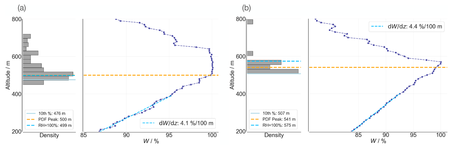
Figure 3 First ceilometer cloud returns for 30 min before and after the radiosonde launch time (grey histograms) and the relative humidity profiles measured by the radiosondes (blue profiles, data every 10 m). Also shown on the ceilometer cloud base height histograms are the 10th percentile (solid light blue line), the first major peak of the distribution calculated from a Gaussian kernel density estimate (orange dashed line), and the height at which relative humidity would reach 100 % when extrapolating from a linear regression fit to the observed profile from 200–400 m (turquoise dashed line), as described in the text. Panel (a) is around the radiosonde launched on 29 January 2020 at 06:44 UTC (02:44 a.m. local Barbados time) and panel (b) is 1 February 2020 at 00:25 UTC (08:25 p.m. local Barbados time). These are two cases where radiosonde relative humidity reached 100 % below 1000 m.

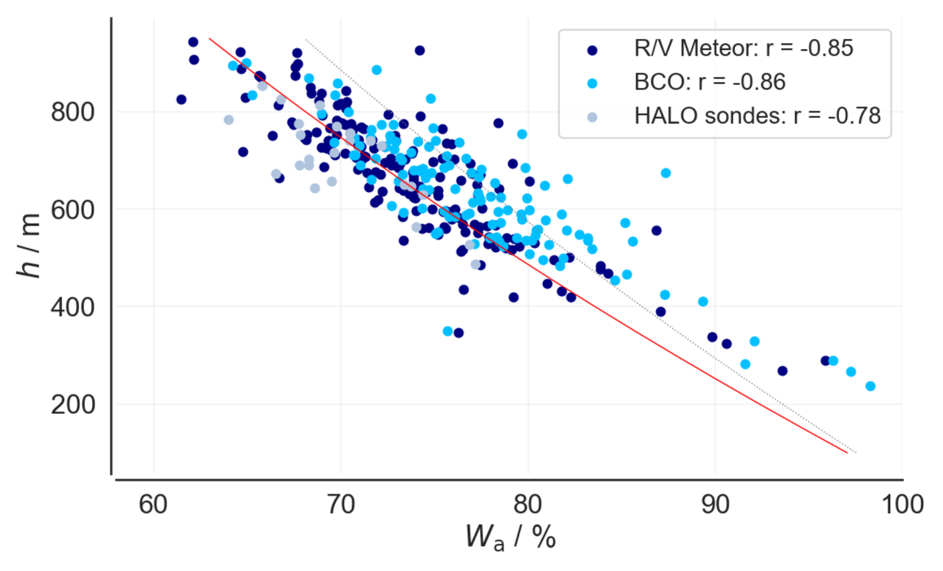
Figure 4 W_a from radiosondes and ceilometer-based estimates of h (using the first, major peak of the distribution), from R/V Meteor (n=171, dark blue) and BCO (n=118, medium blue) measurements. Also shown are area averaged estimates of h from HALO dropsondes (light blue) as calculated by Vogel et al. (2022) and Albright et al. (2022). Lines are theoretical relationships, as described in the text (red: adiabatic lapse rate of −9.8 K km⁻¹; light grey dashed line: temperature lapse rate of −8.5 K km⁻¹).

Using the first distribution peak of ceilometer values to estimate h, we calculate h and W_a for 118 radiosondes at the BCO and 171 radiosondes at the R/V Meteor. Figure 4 shows the close association between these two quantities. Also shown for comparison are subcloud layer height estimates from dropsonde measurements and virtual potential temperature, θ_v, vertical profiles (averaged at the ∼ 220 km diameter circle spatial scale, over three hours, following Vogel et al., 2022 and Albright et al., 2022). Theoretical estimates from Eq. (4) are also plotted, both the adiabatic case and a case where $\frac{\mathrm{d}T}{\mathrm{d}z}$ departs from its adiabatic profile. The agreement between the lines and the points in Fig. 4 show the expected consistency.

4.2 Testing the method with airborne lidar data

Having established the relationship between h and W_a based on both theory and surface measurements, we now turn to estimating the relationship using data from WALES airborne data. For each profile, the lowest altitude where the lidar signal is above background aerosol values is selected using a backscatter ratio of 20. The threshold for the backscatter ratio was set to 20 to ensure it lies well above values typically associated with strong aerosol loadings, which can reach up to around 10 for transported desert dust. Lowering the threshold would identify more clouds; however, the resulting change in relative humidity is minimal (about 1 % when varying the threshold from 10 to 20) and becomes negligible (around 0.1 %) when increasing it further from 20 to 40. We only consider cases where the sea surface is still visible, which ensures the accuracy of the extinction correction by the HSRL method. This consideration limits detections to optically-thin clouds or the corner regions of clouds, as deeper clouds are opaque to the downward-staring lidar, and has the advantage of being less susceptible to rain detections. For edge cases this implies that the cloud base near the edges of the clouds can be extrapolated to the center of the cloud, which is opaque to the lidar (e.g., assuming that the clouds are mostly flat at the bottom). For multi-layered cloud systems, the base of the upper layer is sometimes identified instead of the lowest cloud base. These cases could be flagged and removed based on a cloud base height histogram controlled filter which uses the fact that for multilayer systems a second or third mode appears. As discussed above in the case of surface-based measurements, 3D effects can also bias cloud bases high when the cloud is vertically skewed by wind shear, a situation that Nuijens et al. (2014) showed was not uncommon for the winter trades near Barbados. In this case the lidar will at times only intersect the top cloud base region. We minimize these effects by applying a running minimum filter with a width of 3 km.

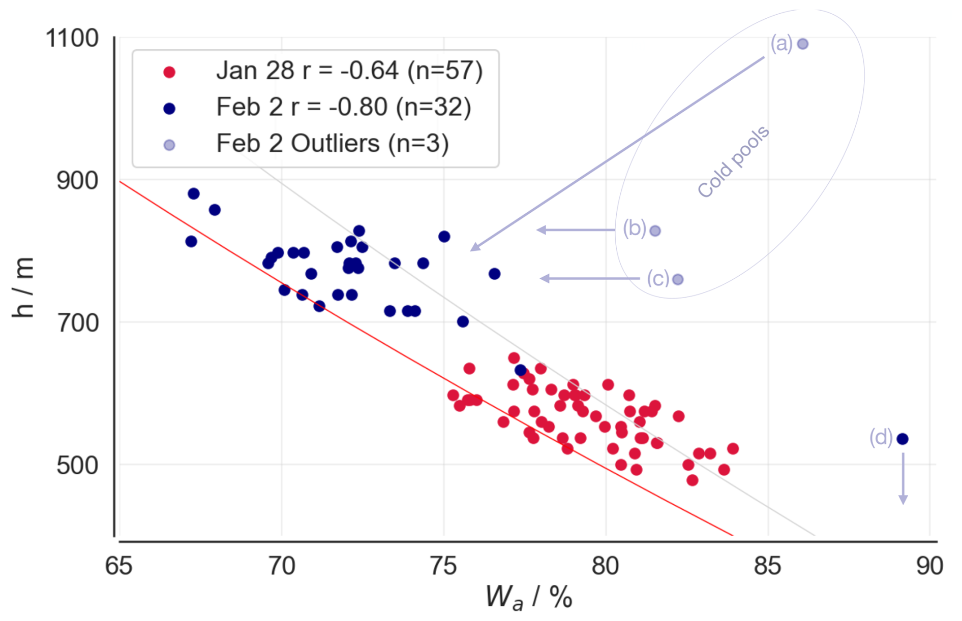
Figure 5 h from WALES for two days, 28 January (red) and 2 February 2020 (blue), and W_a from the nearest dropsonde launch. Outliers are labeled, with the suspected source of bias as suggested in the text. As in Fig. 4, lines are theoretical relationships (red: adiabatic lapse rate of −9.8 K km⁻¹; light grey line: temperature lapse rate of −8.5 K km⁻¹).

Figure 5 presents results for two days of the campaign: 28 January 2020 (57 WALES lidar–dropsonde pairings) and 2 February 2020 (32 pairings), which are selected because they sampled a representative range of different cloud base conditions. 28 January was characterized by small cumulus clouds, often referred to as “sugar” clouds (e.g., Stevens et al., 2020; Bony et al., 2020), while 2 February was characterized by deeper clouds with more stratiform layers near cloud top, often referred to as “flower” clouds (e.g., Stevens et al., 2020) and the presence of a strong Saharan dust layer reaching up to 2.5 km. Overall there is a good correspondence between h as measured by WALES and the dropsonde W_a, all the more so given that the W_a is a point estimate not necessarily centered on the lidar estimates.

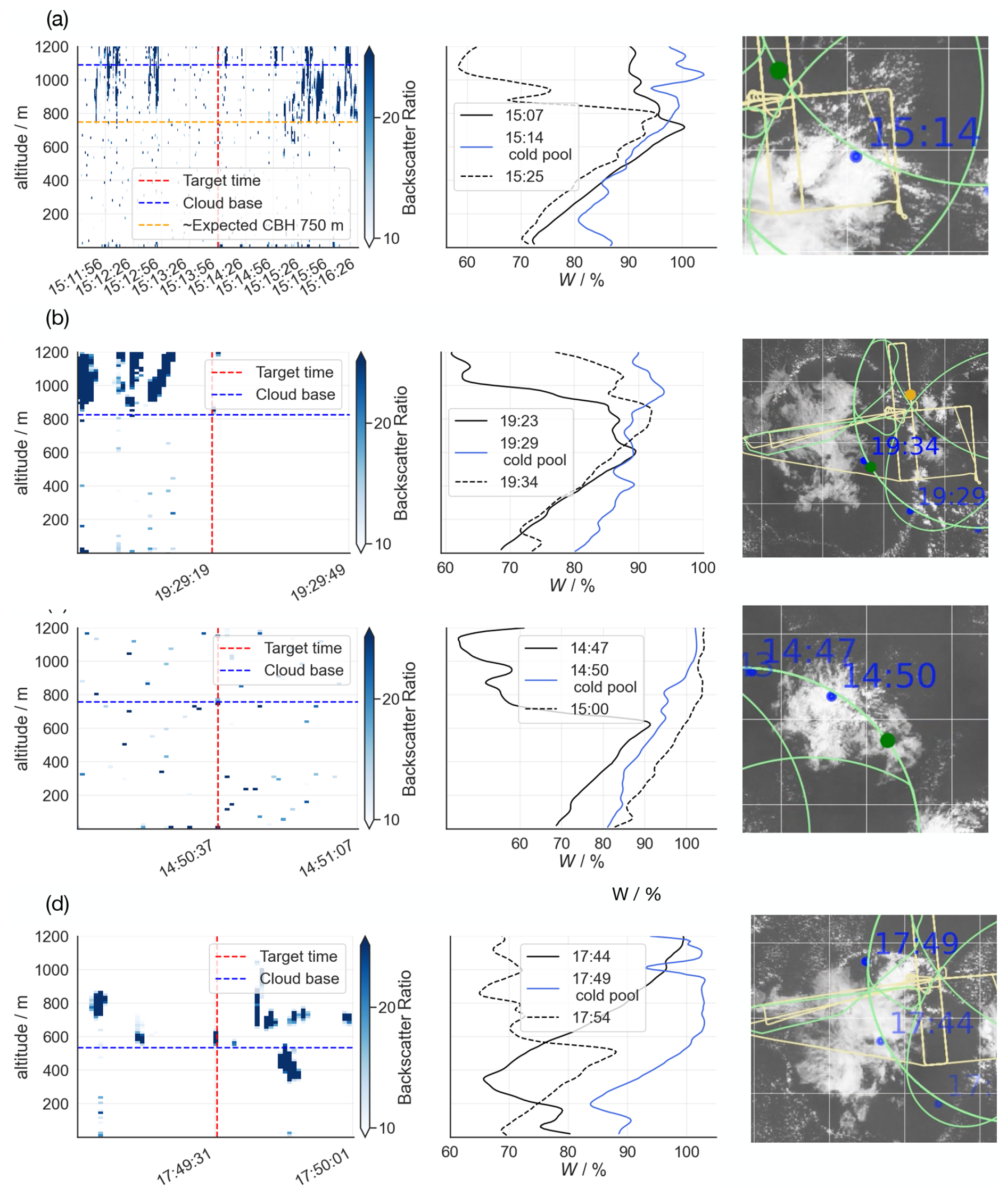
Figure 6 Four anomalous W_a, h pairings from Fig. 5. Shown for the four outlier points are: (left column) the backscatter ratio including the selected time as vertical line (red), the inferred cloud base height (blue horizontal line), and for the top panel, an approximate cloud base height value expected from the linear relationship (orange horizontal line); (center column) relative humidity profiles for the nearest sounding in blue, as well as the soundings immediately before and after (black, solid and dashed, respectively); (right column) visible satellite images (GOES-16 ABI) showing the cloud structure from above and the location of the dropsonde at its launch time, accessed via https://observations.ipsl.fr/aeris/eurec4a-data/PRODUCTS/GOES-E_movies/VIS_IR_combined/v1.0.0/ (last access: 5 July 2026).

A few outliers from the rest of the data are apparent in Fig. 5. An analysis of these exceptions helps give confidence in the rule, i.e., the purported W_a(h) relation. For the 2 February 2020 case, which had more stratiform clouds, three outliers are identified. To investigate these outliers, we examine the backscatter data used to estimate the cloud base height, vertical profiles of relative humidity for the closest dropsonde and the dropsondes immediately prior and after, and visible satellite images of the cloud formations (Fig. 6). A visual inspection of the scenes around the anomalous points suggest that the outliers are associated with cold pools that increase relative humidity (increasing specific humidity and decreasing temperature) (Touzé-Peiffer et al., 2022), and/or cloud fragments associated with dissipating or stratiform cloud elements. The outlier labeled (a) appears to be a cloud fragment from the stratiform cloud layer, as seen in the backscatter ratios and, to some extent, in the visible satellite image; it is associated with higher relative humidity than the dropsonde sounding immediately before and after. If instead estimating a cloud base height around 750 m and relative humidity between 70 %–75 % representative of the larger environment, the point would align with the other data, as illustrated schematically in Fig. 5. Cases (b) and (c) correctly identify the cloud base height, but the cold pool soundings have higher-than-expected relative humidity as seen in the dropsonde profiles. This high value of W_a result in a W_a(h) relationship that differs from the expected linear relationship, but these values would not be expected to be associated with significant errors in the inferred relative humidity because the cloud base height estimate is not biased. Having removed these outliers on 2 February, the WALES lidar method has similar skill to ground-based lidar estimates as shown in Fig. 4.

In addition, point (d) in the figure appears to be associated with cloud forming on a cold pool boundary, which was uncharacteristic of the broader cloud environment (Fig. 6d). Here again it appears that the value does not violate the W_a(h) relationship being used to infer W_a from h, but rather violates the correspondence between the humidity estimate and the lidar selection of the lowest cloud base. Recalculating the correlation with a cloud base height value of 300 m, the association increases (to $r=-\mathrm{0.86}$). This example suggests some ambiguity in the estimate of W_a based on the spread of cloud base estimates below the peak value of the distribution, something that would have to be fine-tuned in an operational retrieval.

4.3 Estimates of $\frac{\mathrm{d}W}{\mathrm{d}z}$ and Δ_aT

To operationalize our framework requires estimating the two near-surface control parameters, $\frac{\mathrm{d}W}{\mathrm{d}z}$ and Δ_aT, from observations and adopt representative values to convert W_a(z_a) into q_s−q_a in the analysis. To test the proposed method we use the EUREC⁴A data. If these ideas were used to develop an operational product, they may need to be tuned, perhaps to depend on ambient conditions from a prior expectation or other product.

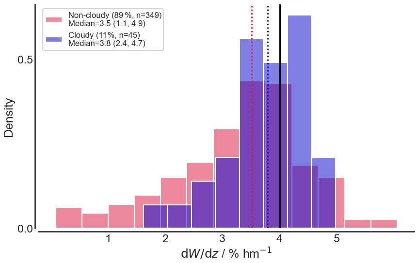
Figure 7 Histograms of $\frac{\mathrm{d}W}{\mathrm{d}z}$ calculated from R/V Meteor soundings as a linear regression between 200 and 400 m: cloudy soundings (blue), defined as soundings where W≥100 % below 1 km, and non-cloudy soundings (red) otherwise. Vertical dashed lines mark the median of each distribution, and the solid black line marks the representative value of 4  % hm⁻¹ used in the analysis.

Figure 7 shows the distribution of relative-humidity lapse rates, $\frac{\mathrm{d}W}{\mathrm{d}z}$, calculated from R/V Meteor radiosondes launched between 16 January and 1 March 2020. Soundings are separated into cloudy profiles (where W reaches 100 % below 1 km) and non-cloudy profiles. The lapse rate is estimated from a linear regression between 200 and 400 m. For cloudy soundings, which occur about 10 % of the time, the mean is 3.9 % hm⁻¹ (median 3.8 % hm⁻¹; 5 %–95 % range 2.4 to 4.7 % hm⁻¹). For non-cloudy soundings, the distribution is broader with a median of 3.5 % hm⁻¹ (5 %–95 % range 1.1 to 4.9  % hm⁻¹).

These empirical estimates agree closely with the theoretical expectations derived in Sect. 3, where Eq. (3) predicted an adiabatic rate of $\frac{\mathrm{d}W}{\mathrm{d}z}\approx \mathrm{4.0}\mathrm{\%}{\mathrm{hm}}^{-\mathrm{1}}$ and Eq. (4) gave a slightly smaller non–well-mixed value of about 3.6 % hm⁻¹. Based on these results, in the subsequent analysis, we adopt $\frac{\mathrm{d}W}{\mathrm{d}z}=\mathrm{4}\mathrm{\%}{\mathrm{hm}}^{-\mathrm{1}}$ as a representative value – close to both the peak of the cloudy-sounding distribution and the theoretical estimate.

For z_a=40 m, Δ_aP≡P_s−P_a is negligible compared with P. Given W_a, we can therefore calculate q_s−q_a from $h\frac{\mathrm{d}W}{\mathrm{d}z}$ and Δ_aT. Because both $\frac{\mathrm{d}W}{\mathrm{d}z}$ and Δ_aT are controlled by boundary-layer dynamics and the near-adiabatic temperature structure, both quantities are expected to remain relatively constant over time.

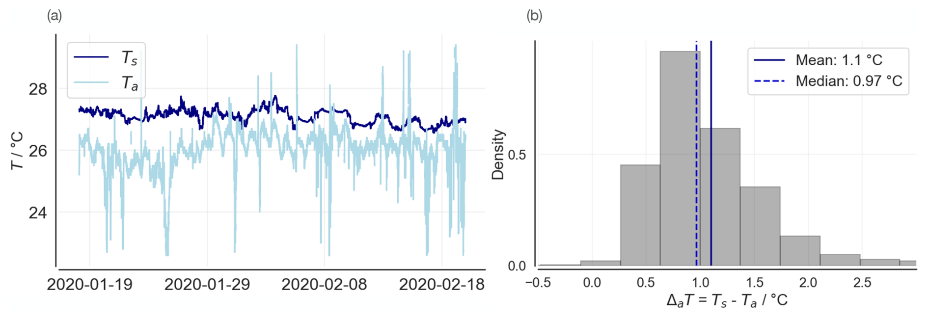
Figure 8 (a) Time series of sea-surface temperatures (T_s), measured 5 m below the ocean surface, and near-surface air temperatures (T_a), measured at 28.3 m on the R/V Meteor. (b) Distribution of differences between the measured (bulk) sea-surface and near-surface air temperatures, with vertical lines for the mean and median values.

Figure 8a shows the time evolution of sea-surface temperatures measured by the port thermosalinograph (depth 5 m) and near-surface air temperatures measured at 28.3 m. The seawater measurements are expected to be biased warm relative to the true skin temperature due to the cool-skin effect, typically 0.1 to 0.3 K (Fairall et al., 1996a; Yan et al., 2024). As expected, nearly all (97 %) of the 47 512 measurements show the ocean is warmer than the overlying air, consistent with unstable and convective conditions. The median and mean temperature differences are 1.0 and 1.1 K, respectively. Because the relevant temperature for surface fluxes is the sea-surface skin temperature, which is approximately 0.2 K cooler than the measured bulk temperature (Fairall et al., 1996; Yan et al., 2024), we adopt a representative offset of Δ_aT=1.0 K. In practice, the near-surface air temperature at each radiosonde launch is obtained by subtracting 1.0 K (the mean bulk-air difference referenced to z_a=40 m) from the measured bulk sea-surface temperature. The retrieved q_a is not sensitive to the precise choice, changing by about 0.1 g kg⁻¹ per 0.1 K in Δ_aT (Eq. 8).

Because bulk flux algorithms may be formulated to use either a skin temperature or a bulk (foundation) temperature as input, consistent treatment of cool-skin and warm-layer effects is important when translating Δ_aT into latent heat flux estimates. Omitting a cool-skin adjustment can lead to mean latent heat flux differences exceeding 6 W m⁻² when the bulk formulation expects a skin temperature (Cronin et al., 2019). Recent updates to the COARE framework include an updated treatment of the cool skin effect (Fairall et al., 2026). While we adopt a fixed representative offset here for consistency and simplicity, we note that an operational implementation of the present retrieval would benefit from coupling the humidity estimate to a physically based cool-skin and warm-layer correction scheme.

4.4 Retrieval skill in q_a

We now evaluate the retrieval skill of the cloud base-height method for near-surface specific humidity, q_a, by comparing predicted values with co-located sounding observations. Figure 9a and b present the predicted near-surface specific humidity, q_a, based on 171 co‐located ceilometer–radiosonde pairs and observed radiosondes launched from the R/V Meteor. On average the cloud base height method overestimates q_a by 0.43 g kg⁻¹ (5th–95th percentile range: −0.65 to 1.9 g kg⁻¹), with a median absolute error of 0.52 g kg⁻¹. The temporal variability is well captured (r=0.76). The largest positive biases occur early in the campaign when cloud bases were low – the error in q_a correlates with cloud‐base height (r=0.54 overall, rising to r=0.76 for bases below 600 m), suggesting that shallow, poorly mixed layers (e.g., beneath decaying cold pools; see Fig. 6) are less amenable to this approximation. No systematic diurnal bias is evident, although the small sample size limits a definitive assessment of hour‐of‐day effects.

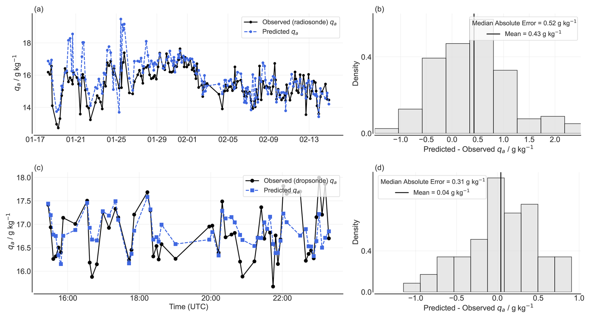
Figure 9 Comparison of observed and predicted near-surface specific humidity estimates and their error distributions. (a) Time series of observed q_a from radiosondes launched from the R/V Meteor (solid black) versus the cloud base-height-derived prediction from R/V Meteor ceilometer data (dashed blue; r=0.76). Time is month and day. (b) Histogram of predicted minus observed q_a for the R/V Meteor data with a median absolute error of 0.52 g kg⁻¹ and a mean bias of 0.43 g kg⁻¹ (vertical line). (c) Time series of observed q_a from HALO dropsondes (solid black) versus cloud base-height-derived predictions from WALES airborne lidar estimates on 28 January 2020 (dashed blue, r=0.61). Time is hour and minute, UTC. (d) Histogram of predicted minus observed q_a for the HALO comparison, with a median absolute error of 0.31 g kg⁻¹ and a mean bias of $-\mathrm{0.04}\mathrm{g}{\mathrm{kg}}^{-\mathrm{1}}$ (vertical line).

Figure 9c, d shows the comparison between WALES airborne lidar–derived q_a estimates and coincident dropsonde measurements also from HALO. Here the cloud‐base method again reproduces the variability reasonably well (r=0.61), with a small mean bias of 0.04 g kg⁻¹ and a median absolute error of 0.31 g kg⁻¹ on 28 January 2020. On 2 February 2020, the correlation is slightly lower (r=0.57), with a mean bias of $-\mathrm{0.06}\mathrm{g}{\mathrm{kg}}^{-\mathrm{1}}$ and a median absolute error of 0.31 g kg⁻¹.

5 Scope, caveats, and practical use

The method proposed in this study is designed for convective marine boundary layers in which the subcloud layer is well mixed and shallow cumulus clouds are coupled to the surface. These conditions are ubiquitous over the world ocean (Fig. 1). Under such conditions, the cloud base height corresponds closely to the lifting condensation level, which depends primarily on the near-surface temperature and humidity.

Despite the ubiquity of favorable conditions, several processes can violate the proxy's assumptions or introduce measurement bias. Cold pools from downdrafts and rain-driven outflows can produce shallow, moist layers decoupled from the overlying cloud, lowering the observed cloud base relative to the environmental LCL and thus overestimating q_a. Optically thick or multilayer clouds pose observational limits: a lidar or ceilometer may detect an upper cloud base rather than the lowest, inflating the apparent cloud base height and biasing the inferred near-surface humidity low; optical-depth and multilayer screening are therefore required. Shallow or weakly mixed layers, in addition to those induced by cold pools, depart from the well-mixed assumption, weakening the cloud base and surface-humidity link and typically yielding low-biased estimates of q_a unless filtered.

Accordingly, the proxy should be applied only where boundary-layer conditions are convective and the detected cloud base is the lowest layer coupled to the surface. These conditions can be diagnosed using coincident lidar backscatter, optical-depth screening, or reanalysis-based buoyancy metrics as in Fig. 1. Within such convective marine regimes, the method's assumptions hold and the resulting estimates of near-surface specific humidity are expected to be reliable.

6 Discussion and conclusions

We show that downward-looking lidar retrievals of cloud base height can be used to infer near-surface relative humidity, a key missing ingredient for remote-sensing estimates of the surface water vapor flux. Combined with wind speed, sea surface temperature, and the near-surface air–sea temperature difference, this information enables physically-based estimates of the surface water vapor flux. Over the ocean, where such measurements are both scarce and critical for the surface energy balance, scatterometers provide wind speed, and long-running satellite records provide sea-surface temperature. The air–sea temperature difference varies only modestly over much of the open ocean on monthly and basin scales, and it can therefore often be estimated statistically; however, this assumption breaks down in regions of strong gradients such as western boundary currents, upwelling zones, and frontal regions, where variability is large and direct observations or physically based corrections remain important.

The method we propose for estimating near-surface humidity requires unbiased estimates of cloud base height, and the satisfaction of two further assumptions: (i) that the relative humidity lapse rate is near the value it would obtain in a well-mixed layer, and thus relatively constant; and (ii) that the near-surface air temperature is cooler than the surface, so that the layer above is convectively driven. Convective boundary layer clouds – which form in the radiatively cooled, cold advection-dominated boundary layers that prevail over tropical oceans – both underpin our near-surface humidity estimates and confirm that the very conditions required for those estimates are in place. While this physical situation limits the application of the method to conditions where shallow convective clouds are present, they are ubiquitous, even in regions of deep convection. Our analysis shows that the method will benefit from some calibration for estimating cloud base from a distribution of lidar echoes, for estimating the relative humidity lapse rate, and for estimating the air-sea temperature difference. Their unbiased estimation will be required for using the proposed method to establish large-scale climatologies of near-surface relative humidity and associated moisture fluxes.

Finally, we note that improving q_a addresses only one, albeit dominant, term in Eq. (1). For latent heat flux applications, residual uncertainties will remain associated with wind speed retrievals and with the wind- and stability-dependence of the exchange coefficient, C. In particular, low-wind conditions require special treatment in many bulk algorithms (e.g., convective gustiness terms), and high-wind conditions can involve additional processes (e.g., sea state and spray) that affect transfer coefficients. Thus, the value added by a cloud base–constrained humidity estimate should be assessed jointly with wind-speed regime and the chosen bulk parameterization when developing and evaluating flux climatologies.

As an outlook we note that the method we propose could facilitate the development of a long-term, day and night, and physically-based near-surface humidity climatology if applied to global data of cloud base height. Techniques using multi‐angle satellite imagery have been shown to retrieve cloud base height, albeit over longer timescales (Böhm et al., 2019). The most promising candidate for obtaining such data is measurements using a spaceborne lidar. Currently the newly-launched EarthCARE satellite (Illingworth et al., 2015) provides HSR-Lidar data. It provides backscatter data with a horizontal resolution of about 280 m and a vertical resolution of 100 m. While the horizontal resolution appears to be sufficient to apply our method, the limited vertical resolution would imply an error of the near-surface humidity of about 0.5 g kg⁻¹ attributed to the vertical sampling error alone (based on Eq. (9) assuming typical values for W_a,h, etc.). With sufficient sampling, and given the variability of cloud base height, it might be possible to obtain greater precision in estimates of the mean cloud base height than what is implied by the single-snapshot vertical resolution. Laser ranging using more sophisticated methods, such as employed by the Global Ecosystem Dynamics Investigation lidar aboard the International Space Station, could provide better estimates of cloud base height. But presently GEDI does not provide data products that allow this capability to be explored. Future satellites refining these technologies could be adapted to the requirements of our proposed method, and potentially could provide coincident estimates of near-surface wind speed and air-sea temperature difference. In this context, measurements of ocean surface texture using synthetic aperture radar could also be explored as a way to estimate the difference between the surface temperature and that of the air just above it, which would better constrain the proposed estimates both directly, and indirectly due to the expected covariability of the relative humidity lapse rate and the air-sea temperature difference. At the least, our work suggests that cloud base height information from lidar measurements could be usefully incorporated into reanalyses and into existing statistical flux retrieval frameworks – such as those used in HOAPS, SeaFlux, IFREMER, or J-OFURO climatologies (e.g., Gentemann et al., 2020; Liman et al., 2018; Bentamy et al., 2017a; Tomita et al., 2019) – to better constrain near-surface humidity and surface moisture fluxes.

Appendix A: Derivation of the adiabatic relative-humidity lapse rate

Starting from the definition of relative humidity,

$$\begin{array}{}\text{(A1)}& W={\displaystyle \frac{e}{e_{*}\left(T\right)}},\end{array}$$

we take the vertical derivative of its logarithm,

$$\begin{array}{}\text{(A2)}& {\displaystyle \frac{\mathrm{d}}{\mathrm{d}z}}\ln W={\displaystyle \frac{\mathrm{1}}{e}}{\displaystyle \frac{\mathrm{d}e}{\mathrm{d}z}}-{\displaystyle \frac{\mathrm{1}}{e_{*}}}{\displaystyle \frac{\mathrm{d}{e}_{*}}{\mathrm{d}z}}.\end{array}$$

Using the Clausius–Clapeyron relation,

$$\begin{array}{}\text{(A3)}& {\displaystyle \frac{\mathrm{d}\ln e_{*}}{\mathrm{d}T}}={\displaystyle \frac{{\mathrm{\ell }}_{\mathrm{v}}}{R_{\mathrm{v}}{T}^{\mathrm{2}}}},\end{array}$$

the second term becomes

$$\begin{array}{}\text{(A4)}& {\displaystyle \frac{\mathrm{1}}{e_{*}}}{\displaystyle \frac{\mathrm{d}{e}_{*}}{\mathrm{d}z}}={\displaystyle \frac{{\mathrm{\ell }}_{\mathrm{v}}}{R_{\mathrm{v}}{T}^{\mathrm{2}}}}{\displaystyle \frac{\mathrm{d}T}{\mathrm{d}z}}.\end{array}$$

For the vapor pressure term, we write

$$\begin{array}{}\text{(A5)}& e=q{\displaystyle \frac{R_{\mathrm{v}}}{R}}P,\end{array}$$

where $R=(\mathrm{1}-q)R_{\mathrm{d}}+q{R}_{\mathrm{v}}$ is the gas constant of moist air. Taking the logarithmic derivative,

$$\begin{array}{}\text{(A6)}& {\displaystyle \frac{\mathrm{1}}{e}}{\displaystyle \frac{\mathrm{d}e}{\mathrm{d}z}}={\displaystyle \frac{\mathrm{1}}{q}}{\displaystyle \frac{\mathrm{d}q}{\mathrm{d}z}}+{\displaystyle \frac{\mathrm{1}}{P}}{\displaystyle \frac{\mathrm{d}P}{\mathrm{d}z}}-{\displaystyle \frac{R_{\mathrm{v}}-R_{\mathrm{d}}}{R}}{\displaystyle \frac{\mathrm{d}q}{\mathrm{d}z}}.\end{array}$$

Using hydrostatic balance,

$$\begin{array}{}\text{(A7)}& {\displaystyle \frac{\mathrm{d}P}{\mathrm{d}z}}=-\mathit{\rho }g=-{\displaystyle \frac{P}{RT}}g,\end{array}$$

so that

$$\begin{array}{}\text{(A8)}& {\displaystyle \frac{\mathrm{1}}{P}}{\displaystyle \frac{\mathrm{d}P}{\mathrm{d}z}}=-{\displaystyle \frac{g}{RT}}.\end{array}$$

Substituting into Eq. (A2) yields the general expression

$$\begin{array}{}\text{(A9)}& {\displaystyle \frac{\mathrm{1}}{W}}{\displaystyle \frac{\mathrm{d}W}{\mathrm{d}z}}=\left[\left({\displaystyle \frac{\mathrm{1}}{q}}-{\displaystyle \frac{R_{\mathrm{v}}-R_{\mathrm{d}}}{R}}\right){\displaystyle \frac{\mathrm{d}q}{\mathrm{d}z}}-{\displaystyle \frac{g}{RT}}-{\displaystyle \frac{{\mathrm{\ell }}_{\mathrm{v}}}{R_{\mathrm{v}}{T}^{\mathrm{2}}}}{\displaystyle \frac{\mathrm{d}T}{\mathrm{d}z}}\right].\end{array}$$

In a well-mixed, unsaturated subcloud layer,

$${\displaystyle \frac{\mathrm{d}q}{\mathrm{d}z}}\approx \mathrm{0},{\displaystyle \frac{\mathrm{d}T}{\mathrm{d}z}}\approx -{\displaystyle \frac{g}{c_p}},$$

so Eq. (A9) reduces to

$$\begin{array}{}\text{(A10)}& {\displaystyle \frac{\mathrm{1}}{W}}{\displaystyle \frac{\mathrm{d}W}{\mathrm{d}z}}={\displaystyle \frac{g}{T}}\left({\displaystyle \frac{{\mathrm{\ell }}_{\mathrm{v}}}{c_p{R}_{\mathrm{v}}T}}-{\displaystyle \frac{\mathrm{1}}{R}}\right),\end{array}$$

which corresponds to Eq. (3) in the main text.