Validation of EarthCARE CPR reflectivity using the ACTRIS cloud radar network

The Earth Cloud, Aerosol, and Radiation Explorer (EarthCARE) satellite carries a cloud profiling radar (CPR) designed to observe global cloud properties. In this study, we assess the calibration of CPR reflectivity profiles by comparing them with seven calibrated ground-based cloud radars from the European Aerosol, Clouds and Trace Gases Research Infrastructure (ACTRIS).

We compare the statistics of ice cloud reflectivities observed from space and from each ground site. The CPR dataset includes all observations within a 200 km radius of each site, while the ground-based dataset comprises vertical profiles collected during the same time period. For this study, the CPR and ACTRIS data were compared on a period spanning from July 2024 to November 2025. By analysing the differences in reflectivity statistics, we estimate the calibration bias between CPR and each site. To ensure robustness, we implement a method to select height bins with comparable reflectivity statistics, excluding uncorrelated observations that could contaminate the results. The reliability of our bias estimates is validated through closure: each ground radar has been calibrated using the same reference, and the independently derived space-versus-ground biases obtained across sites are consistent. Our methodology also provides uncertainty estimates for the reflectivity biases and explores the time sampling required for reliable comparisons.

Based on the comparisons from the seven ground-sites, we find that the bias in the EarthCARE L2a reflectivity product is of $-\mathrm{0.2}\pm \mathrm{0.4}$ dB, confirming the high quality of the satellite's calibration. This robust statistical approach, validated with calibrated radars, establishes EarthCARE as a potential reference for calibrating ACTRIS and other ground-based sites in the future.

1 Introduction

Launched on the 28 May 2024, the Earth Cloud, Aerosol, and Radiation Explorer (EarthCARE) satellite measures aerosol, cloud, and precipitation profiles alongside their co-located radiative flux at the global scale (Wehr et al., 2023). To this end, it is equipped with a Doppler cloud radar, an atmospheric lidar, a multispectral imager, and a broadband radiometer. The observations from these instruments will be used to evaluate the representation of aerosols, clouds and precipitation in weather forecast and climate models, and help improve their parametrization schemes for the next 10 years.

The onboard Cloud Profiling Radar (CPR) operates at 94 GHz frequency (W-band) and is the first space-borne cloud radar measuring Doppler velocities. EarthCARE CPR is capable of measuring reflectivities down to −35 dBZ in the troposphere, improving 5 dB in sensitivity with respect to the previous CloudSat CPR (Wehr et al., 2023). At the early stage of a satellite mission it is essential for its data and products to be verified and validated. The work presented in this article is part of this CAL/VAL (calibration/validation) effort. Coupled with other CAL/VAL methods (ocean backscattering, airborne radar comparisons, ground based calibrators) (Masuko et al., 1986; Horie et al., 2010, 2025), this work aims to ensure that the reflectivity values measured by the CPR are well calibrated.

The Aerosol, Clouds and Trace gases Research Infrastructure (ACTRIS) is a pan-European research infrastructure producing high quality data and services on short-lived atmospheric constituents and the processes leading to their variability in natural and controlled atmospheres (Laj et al., 2024). ACTRIS is structured around three core themes – aerosols, trace gases, and clouds – and relies on Central Facilities, specializing in each of these scientific areas. Among them, the Centre for Cloud Remote Sensing (CCRES) coordinates expertise in cloud remote sensing.

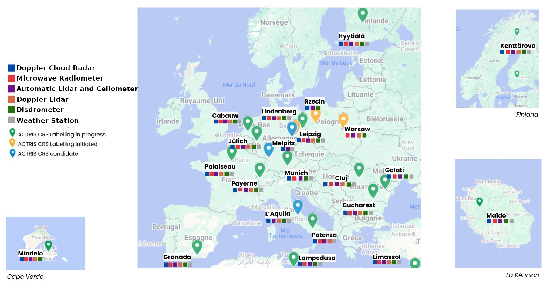
Figure 1 Map of the ACTRIS network of cloud remote sensing sites. Data from the sites of Palaiseau, Jülich, Lindenberg and Leipzig were used in this study. Map edited from Google maps © 2026 Google Maps™ mapping service.

ACTRIS cloud remote sensing sites are mainly distributed in Europe, as shown in the Fig. 1. Most of the sites are equipped with Doppler cloud radars, microwave radiometers, disdrometers, Doppler lidars and ceilometers. This instrumental diversity allows for a variety of products, using the instruments synergy (Illingworth et al., 2007; Tukiainen et al., 2020).

Even with the spatial extension of the ACTRIS network it is, in general, unlikely to have exactly co-localized observations between CPR and ground-based cloud radars. For each site, we expect at least a few tens of kilometres of distance between orbital overpasses and each ACTRIS National Facility (NF). Another consideration is that the majority of ACTRIS ground-based radars are zenith pointing only (∼ 75 %). Even for sites that do have scanning capabilities, co-localization would remain unlikely due to the limited range of cloud radars (≲ 20 km), caused by the strong atmospheric attenuation at their operation frequencies (mainly in the 35 and 94 GHz bands).

We thus adopted a statistical approach to compare the EarthCARE CPR and ground reflectivities. Earlier studies have already proposed methods to do such comparisons, using CloudSat CPR as the space instrument. Both Protat et al. (2009) and Kollias et al. (2019) compare satellite reflectivity profiles, sampled in a given radius around the ground-site of interest, with ground profiles in a fixed time-window around the overpass time. Bias is estimated as the difference between the mean profiles from both sources. These approaches are already capable of providing bias estimates (and hence the calibration difference) between the space and ground instruments, but we find that they can still be improved to provide more robust results in our use-case.

A key limitation of the current approaches is the absence of uncertainty estimates when evaluating bias values. To assess EarthCARE calibration, we compare CPR reflectivity with ACTRIS ground-based radars, which provide calibrated measurements with associated uncertainty estimates. Without accounting for the uncertainty introduced by the satellite-ground comparison algorithm, it is impossible to accurately evaluate the overall uncertainty of our EarthCARE calibration estimates. The quantification and propagation of the uncertainty is then a core requirement for the developed algorithm.

Another key improvement lies in the validation process. For EarthCARE, it is crucial to obtain a reliable calibration estimate that is independent of the characteristics of any single site or specific ground radar. Taking advantage of the calibration homogeneity established by ACTRIS-CCRES, we propose to validate EarthCARE calibration bias estimates using multiple ground-based sites. This enables to further scrutinize the results through closure: having consistent bias estimates from all sites would significantly strengthen confidence in both the data processing methodology and the reliability of the EarthCARE bias estimate.

Another necessary improvement for our use case is the quantification of the minimum sampling time required to ensure reliable comparisons. Currently, no recommended minimum period exists, and given the recent launch of EarthCARE, insufficient data sampling could lead to skewed statistical results. There is a need for a study on how impactful the comparison duration can be on the results.

Finally, our algorithm has to be compatible with EarthCARE and ACTRIS data formats and processing pipelines. This requires adapting the time co-localization in data selection to account for the lower count of vertical profiles compared to raw data from the ground radars. Compatibility with CloudSat data is also desirable to enable historical comparisons with ACTRIS data.

This article is structured as follows. Section 2 is dedicated to the description of calibration strategy of the ACTRIS ground radar network. The satellite and ground datasets are described in Sect. 3. The implemented algorithm and considerations made in its development are presented in details in Sect. 4. The reflectivities of EarthCARE are validated using the calibrated radars from the ACTRIS network, as described in Sect. 5. Section 6 presents the evaluation of the impact of the time period considered for the evaluation of the satellite-ground bias.

2 ACTRIS-CCRES cloud radar calibration strategy

One of the main ACTRIS objectives is to assure reliable, comparable data at all sites of its instrument network. The Center for Cloud Remote Sensing (CCRES) is the ACTRIS expertise center supporting the operations of cloud remote sensing instrumentation within the network (ACTRIS, 2025). A goal of CCRES is to define a set of methodologies to guarantee the highest quality of measurements and data products. CCRES also oversees the deployment and further development of experimental systems dedicated to cloud observation.

CCRES is at present working on a vast calibration effort for the entire ACTRIS cloud radar network. To this end, the strategy involves two parallel activities: (i) To perform the calibration of reflectivity measurements for each radar in the network, and (ii) The implementation of a calibration tracking system which enables detection and quantification of calibration drifts over time.

The reflectivity calibration is done as follows:

1. A portable reference radar (BASTA-CCRES, W-band, Delanoë et al., 2016) is calibrated at a CCRES facility using a reference target (Toledo et al., 2020). The use of targets characterized in an anechoic chamber enables to reach a calibration uncertainty of 0.8 dB on reflectivity.

2. A calibration transfer campaign is organized. The reference radar is sent to another ACTRIS NF to transfer its calibration to the respective local cloud radar(s). The transfer is done by comparing simultaneous vertical cloud profiles observed from a close position, a few tens of meters apart (Jorquera et al., 2023). With this method, a correction coefficient is determined. The correction coefficient can be applied to local reflectivity retrievals to compensate for calibration bias, effectively recalibrating the instrument. The uncertainty of the resulting recalibration depends on the number and type of cloud events sampled, but after eight weeks of campaign one can usually reach values in the range of [±0.9; ±1 dB].

As the described calibration campaign are time consuming, it is necessary to track any change in the calibration of the ground radars. A calibration tracking setup is thus implemented at each ACTRIS NF, in parallel to the calibration campaigns. The setup requires the installation of a co-located disdrometer, with the objective of independently measuring the reflectivity of stratiform precipitating particles. These reflectivity values are then compared with radar observations to detect sudden calibration biases and enable corrective actions, ensuring a reliable data set (e.g. Hogan et al., 2003; Kollias et al., 2019).

Table 1 ACTRIS sites and radars used in this study. From the seven radars used in this study, five were calibrated by ACTRIS-CCRES, and two were recalibrated later based on the already corrected MIRA radar from Julich (indicated with ^*). The calibration of all the instruments is monitored using co-located disdrometers. Ka band radars emit at the 35 GHz band. W band radars emit at the 95 GHz band.

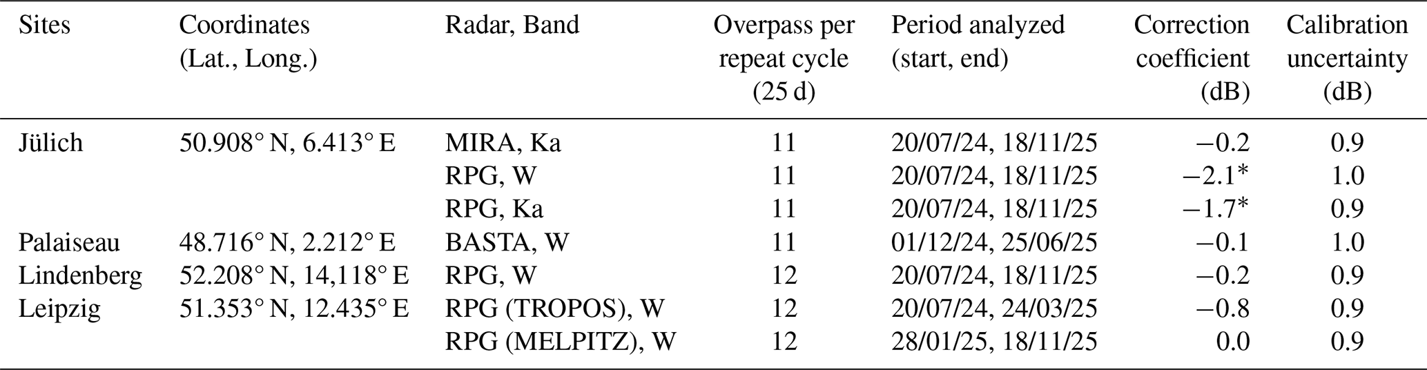
Currently CCRES has completed cloud radar calibration campaigns for the stations of Palaiseau, Jülich, Leipzig and Lindenberg. All radars were calibrated using the BASTA-CCRES reference radar, allowing us to perform closure tests on our space-ground comparison algorithm. Table 1 shows each site coordinates, radar types, number of overpasses within 200 km for each satellite cycle of 25 d, the time period analyzed and the introduced correction coefficient with the resulting ground-radar calibration uncertainty. The two RPG radars of the Jülich site were installed after the calibration campaign took place. Hence their correction coefficients are calculated based on the MIRA radar, which was the only radar in operation at the time of the calibration campaign.

3 Dataset description

In this work, we compare the reflectivity profiles of the EarthCARE L2a CPR FMR products with those sampled by ground-based radars of the ACTRIS network. The following sections present the datasets, and introduces the products that are relevant to our study.

3.1 EarthCARE CPR L2a product

EarthCARE performs 15.5 orbits every 24 h and covers the global surface between latitudes of 83° N and −83° S. The trajectory with respect to Earth's surface drifts slightly with each revolution. This cycle resets every 25 d. Fortunately, we only need that the satellite passes within a 200 km of each ground site (see Sect. 4). This provides a varying amount of 11 to 12 overpasses per satellite cycle (25 d) depending on the site latitude counting both ascending and descending trajectories.

EarthCARE CPR is a W-band radar measuring reflectivities and Doppler velocities from the clouds. The vertical resolution of these observations is 500 m, however the received echo is over-sampled at 100 m. The minimum reflectivity observed by the CPR is −35 dBZ throughout the troposphere. The calibrated radar reflectivities are given in the EarthCARE L1 products (Wehr et al., 2023). Even though calibration accuracy for EarthCARE is still under study, it should have an uncertainty of 0.5–1 dB, based on what was achieved for CloudSat and on the diverse calibration approaches in use (Protat et al., 2009, 2011; Horie et al., 2025). The L1 reflectivity values are corrected for gaseous attenuation in the EarthCARE L2 products.

EarthCARE data are processed on different baselines improving the products with each iteration. The BA baseline is the latest baseline where all the data from the beginning of the mission were reprocessed and thus the one with the most data available. We thus used CPR L2a products of the BA baseline in this study. These data are available from the 20 July 2024 to the 18 November 2025. We decided to use the EarthCARE L2a CPR FMR product because it provides 94 GHz reflectivity values corrected by gas attenuation (Kollias et al., 2023), and the co-localized CPR TC product, providing a target classification (Irbah et al., 2023) allowing a precise profile selection (see Sect. 4.3). All of the data were acquired from the EarthCARE ESA MAAP service (European Space Agency (ESA), 2026). We did not use the EarthCARE radar-lidar (AC-TC) classification product as it as known issues for the classification of some liquid clouds on the BA baseline (and therefore on our time period) (EarthCARE-DISC, 2025).

3.2 ACTRIS-CCRES data centre

The ground-based radar data used in this study were provided by the ACTRIS CloudNet Cloud Remote Sensing Data Centre Unit (CLU), operated at the Finnish Meteorological Institute (FMI) in Helsinki, Finland. This unit serves the ACTRIS cloud remote sensing network by providing numerous services around the data generated by the observation platforms. The CLU services include the centralised data processing to generate multi-instrumental observational and geophysical products, and the implementation of tools for data quality control checks, data harmonisation, data access and data archiving (Illingworth et al., 2007; Tukiainen et al., 2020). All these processes are done by CLU and data are available on the CloudNet data portal (Finnish Meteorological Institute, 2026). These services are especially important for a network such as ACTRIS, due to its large amount of sites and instruments diversity. The cloud radars in the network operate at either the Ka or W band (35 and 95 GHz respectively) and are built by different manufacturers.

The CLU products used in this study are the L2 Categorize product and the L2 Target Classification product (Hogan and O'Connor, 2004). The Categorize product provides vertical cloud radar reflectivity profiles corrected by gas attenuation, with a time resolution of 30 s and a vertical resolution between 25 and 50 m, depending on the specific instruments. The Target Classification product is built with the same resolutions than the Categorize product. These classifications are built using radar, lidar and microwave radiometer data.

At present, CLU is working on a solution to track calibration history at each radar site. While this development is being implemented, the reflectivity values provided in the Categorize product correspond to the original measurements of each radar before recalibration. Thus, for this study, we take these original reflectivity values at each site and correct them manually using the correction coefficients determined in our calibration campaigns (explained in Sect. 2).

4 Ground-space calibration algorithm

4.1 Overview of the algorithm

The location of the ACTRIS cloud remote sensing sites has been established long before the planning of EarthCare orbits, and has been decided by each operator, based on their scientific interests and local constrains. They have usually been placed on previously existing atmospheric observatories (Laj et al., 2024). As EarthCARE has a revisit time of 25 d, the overpasses distances are fixed. For example, for the 4 calibrated sites used for this study, the closest overpasses are for the Lindenberg site with overpasses every 25 d within 3 km to 400 m from the site. The Julich site also have very close overpasses in a few km range, but the 2 other sites of Palaiseau an Leipzig do not. It is therefore very unlikely to have situations where direct comparisons of co-localized clouds are possible. Moreover, as mentioned in Sect. 1, the use of scanning radars would not be a viable strategy for the validation of the reflectivities at the scale of the ACTRIS network. Hence a statistical comparison algorithm is implemented, based on the following considerations:

1. Previous studies have found that on a certain time period, ground and satellite radars mean profiles will show statistical similarities (Protat et al., 2009; Kollias et al., 2019). In these studies, the CloudSat CPR reflectivity profiles are selected in a 200 km radius around the ground sites and the ground profiles in a ± 1 h period around the overpass time, independently of the sites geographical position. Testing the radius criteria parameter, we found that 200 km is a suitable distance for the comparisons at European latitudes. However, the selection of ground profiles in a ± 1 h period around the overpass is limiting for our comparisons. For the ground data we thus use all the profiles observed on the time period considered for the comparison. The assumptions on this selection of the ground profiles are developed in Appendix A. Comparing both selection criteria we find compatible satellite-bias results.

2. As stated in Sect. 3, the satellite and ground reflectivities used in this study are already corrected for gas attenuation. Moreover, ice clouds observed from the satellite (seeing clouds from the top) will remain largely unattenuated, while ice clouds observed from the ground (seeing the clouds from the bottom) will be strongly attenuated by any liquid clouds bellow it. To avoid the need of correcting the attenuation from liquid water clouds or precipitation, we only concentrate on ice layers since they introduce a negligible attenuation (Matrosov, 2009). Finally we admit that ice clouds are relatively homogeneous targets. Hence, ice clouds are considered the best targets for the comparisons.

To summarize, this study relies on the comparison of the ground site ice clouds reflectivity statistics with the ice clouds reflectivity statistics observed from the satellite. With enough observation time the satellite observations should tend to the same statistics as the one observed from the ground.

Figure 2 Flowchart of the algorithm. Each step is described in the Section in parentheses.

Previous studies show that the statistical similarities between the satellite and ground mean reflectivity profiles only exists at certain heights (Protat et al., 2009; Kollias et al., 2019). Our approach acknowledges this height dependence with the implementation of a method to evaluate the height bins where the ground and satellite reflectivities are the most statistically comparable. The reflectivity comparisons are done on these height bin.

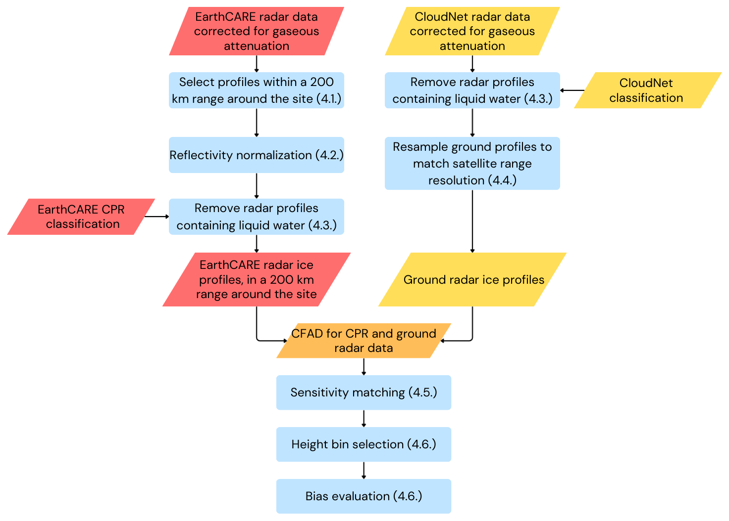
An overview of the developed algorithm is shown as a flowchart in Fig. 2. For a given time period, all satellite data within a 200 km radius of the considered ground site is selected. For the ground data, the ice profiles for all the days in the considered time period are selected, whether or not an overpass occurs on the same day. This allows to set the reflectivity statistics of the site. All the data for a given period are then treated as follows.

On the selected CPR data, we perform a correction to account for the different dielectric constants used when calculating reflectivities with ground and satellite-based radars (see Sect. 4.2). Then, all profiles that contain liquid water are removed using EarthCARE L2a target classification. More details are presented in Sect. 4.3.

For the ground-based data, we firstly remove profiles that contain liquid water, using the CloudNet target classification (see Sect. 4.3). The remaining ground profiles are then resampled to match satellite range resolution as described in Sect. 4.4.

By adding up all the profiles from a period, a contoured reflectivity frequency by altitude diagram (CFAD) is constructed. From the CFADs, both radar sensitivities are matched, without assuming calibrated values for any radar. This is to make sure that we only compare cloud samples that can be observed by both instruments, without biasing a priori the estimated difference in reflectivities. This part of the algorithm is explained in details in Sect. 4.5.

The reflectivity distribution is then fitted with a Gaussian model for each height bin. The parameters from this fit are tested to select statistically comparable height bins. The bias between ground and satellite data is then inferred on these selected height bins. This fitting, height selection and bias evaluation process is detailled in Sect. 4.6.

To support the description of these processes, the data of the RPG94 from the site of Jülich is taken as an example for the figures throughout this section.

4.2 Reflectivity normalization for the dielectric water constant

As mentioned in Sect. 3 both L2a CPR reflectivities and ground radars reflectivities have already been corrected for gaseous attenuation. It is then needed to normalize the CPR reflectivities to acknowledge the difference of dielectric constant between satellite and ground observations.

The difference in dielectric constant is addressed by normalizing the EarthCARE reflectivities, using Eq. (1) (from the radar equation), with K_ground=0.86 and K_EarthCARE=0.75 (Pfitzenmaier et al., 2025).

$$\begin{array}{}\text{(1)}& Z_{\mathrm{EarthCARE}}=Z_{\mathrm{EarthCARE}}-\mathrm{20}{\log }_{\mathrm{10}}\left({\displaystyle \frac{K_{\mathrm{ground}}}{K_{\mathrm{EarthCARE}}}}\right)\end{array}$$

4.3 Ice profiles selection

As ground and satellite have different geometries of observation, the signals are not attenuated in the same way when liquid water is observed. Moreover as mentioned in Sect. 4.1, the attenuation introduced by ice clouds is negligible. As a consequence, to ensure that both datasets are comparable profiles containing liquid water need to be removed for both satellite and ground data. To this end the EarthCARE CPR TC (target classification) product is used for satellite data and the CloudNet classification product is used for the ground data. In addition, we need to consider that some radars in the network don't have blowers to remove the water on the radome after precipitation leading to attenuation. To take this effect into account all the ground data are removed 6 h after a precipitation event, to allow the radome to dry. For the radars used in this study, only the BASTA of Palaiseau is concerned with this problem.

For CloudNet data a profile is removed if one of the following value is present in a profile: cloud liquid droplets only, drizzle or rain, drizzle or rain coexisting with cloud liquid droplets, melting ice particles coexisting with cloud liquid droplets.

For EarthCARE data a profile is removed if one of the following value is present in a profile: liquid cloud, drizzling liquid cloud, warm rain, cold rain, melting snow, heavy rain likely, heavy mixed-phase likely, heavy rain, heavy mixed-phased, rain in clutter, snow or mixed-phased in clutter.

4.4 Ground data resolution resampling

The EarthCARE CPR effective vertical resolution is 100 m. As mentioned in Sect. 3.2, ground radar resolutions are between 25 and 50 m. Thus, it is needed to match both resolutions before performing the comparisons. The resampling of the ground data to the satellite vertical resolution is made using the method described in section 2.4.3 Radar instrument model from Donovan et al. (2023).

For each day, a minimum detectable signal (MDS) curve is given in the CloudNet categorize files, taking account of the effects of ground clutter and gas attenuation. This curve resolution is also resampled to the CPR resolution and is used to remove invalid ground-based samples (usually artifacts from the resolution conversion).

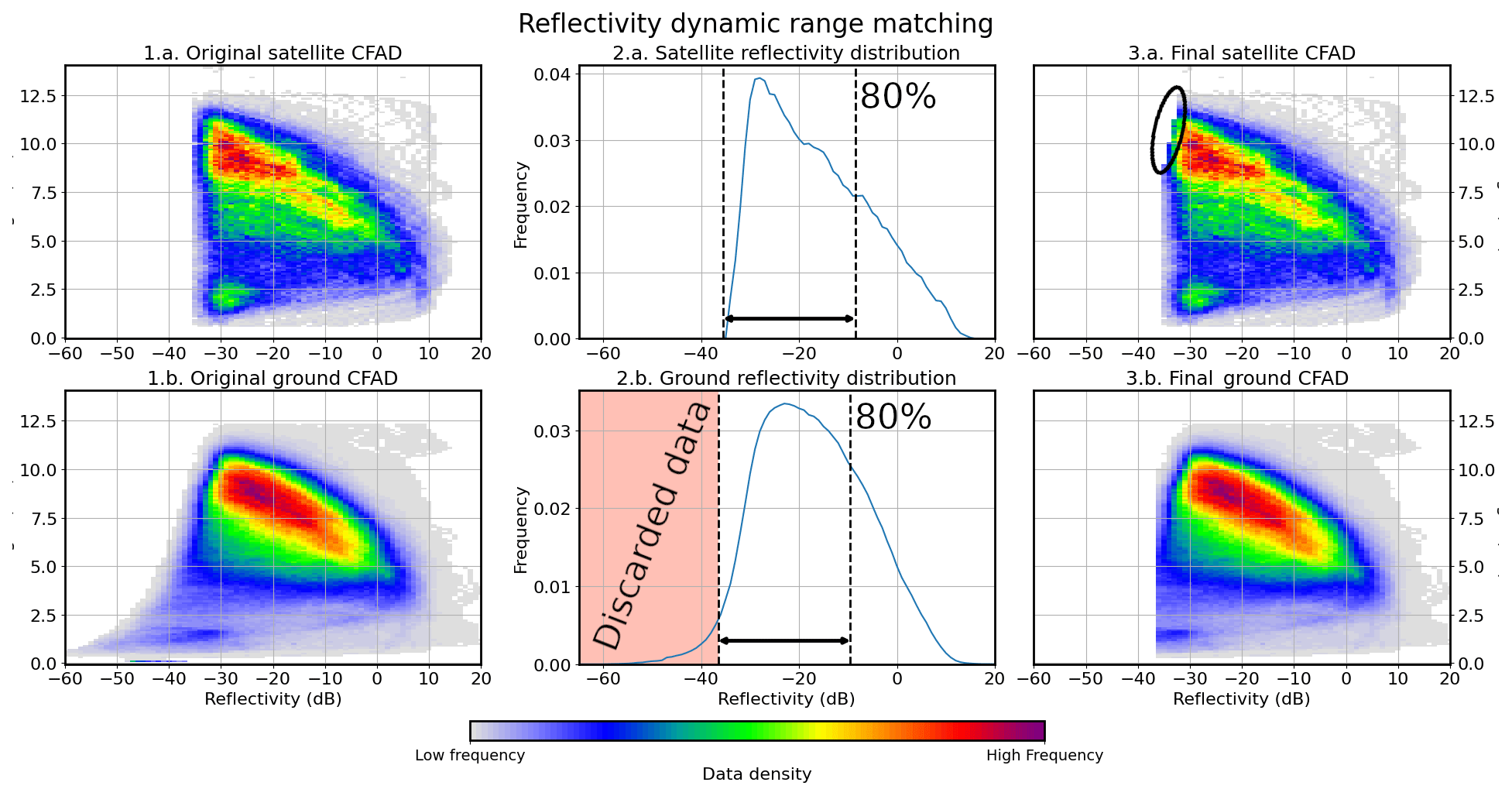
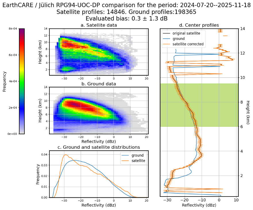
Figure 3 Example of the CFADs and MDS matching for the CPR and ground radar for the RPG94 of Jülich. The CFADs were obtained by collecting all ice profiles on a time period from July 2024 to Novemeber 2025. For the satellite, 14 846 profiles were used. For the ground, 198 365 profiles were used. Panels (1.a.) and (1.b.) show the raw CFADs of both the CPR and the ground radar. The satellite CFAD shows a local maximum of reflectivity frequency around −30 dBZ at an altitude of 2.5 km. This maximum is likely due to second-trip echo effect occurring highly reflective surface on the ground (lake, rivers, ponds, …). These second trip echoes are not filtered, this however does not impact the satellite-ground bias evaluation (see Fig. 5). Panels (2.a.) and (2.b.) show the reflectivity distributions of the satellite and the ground inferred from the CFADs. In panel (2.a.) the satellite reflectivity dynamic range is represented by the double-headed arrow between the black vertical dashed lines, each representing the minimal CPR reflectivity and the 80th percentile of data. The reflectivity dynamic range is then applied on the ground distribution from the 80th percentile of the ground data as shown in panel (2.b.) The red zone represent the discarded data. Panels (3.a.) and (3.b.) show the final CFADs when both reflectivity and power dynamic range were applied. The black circle in panel (3.a.) shows where the data were removed by the matching of the power dynamic range.

4.5 CFADs and sensitivity matching

Using all the satellite and ground profiles selected through the described process, a contoured reflectivity frequency by altitude diagram (CFAD) for the CPR and ground radar is constructed (Fig. 3.1.a. and 1.b.). The sensitivity difference between the ground and satellite radars needs to be addressed. The CPR reflectivity MDS is constant at −35 dBz throughout the troposphere, while for the ground radar the reflectivity MDS decreases with the square of the range from the radar. In contrast, the MDS in power of the ground radar is constant while for the CPR, it decreases while approaching the ground. To match the sensitivity of both instruments we thus need to match their MDS in reflectivity and in power.

From the CFADs, a reflectivity distribution is inferred for both the ground and the satellite (Fig. 3 panel 2). Cutting the minimum reflectivity of the ground distribution to the minimum of the satellite distribution could remove valid data from the comparison if a bias exist between the two distributions. It is therefore preferable to apply the satellite dynamic reflectivity range on the ground distribution to cut it. The dynamic reflectivity range of the satellite is the window between the maximum and minimum reflectivity values observed. Cutting the ground distribution using the satellite dynamic reflectivity range is equivalent to matching the maximum of the distributions and cutting the ground at the minimum of the satellite distribution. However, the two distributions cannot be matched at the maximum reflectivity as the 2 radars do not necessarily observe the exact same cloud. To mitigate this problem we match the dynamic range between the satellite MDS value and the 80th percentile of data (Fig. 3.2.a. and 2.b.). As the 80th percentile of both dataset might not be coincident, this windowing can lead to non coincident minimum reflectivities between both datasets.

From the reflectivity distributions pseudo-power distributions are inferred for both the ground an satellite. As CloudNet categorize and EarthCARE L2a files do not include raw power measurements, the pseudo-power distributions are calculated proportional to the physical power by removing 20log ₁₀(r_ground) (with r_ground the range from the ground radar) from the reflectivities. As stated, the ground data have a constant minimum power, the ground dynamic power range is thus applied on the satellite data the same way than for the reflectivity range. The pseudo-power distributions are not shown as a very low amount of data is discarded through the matching of the power dynamic ranges. However the black circle on the satellite CFAD in panel 3.a. of Fig. 3 shows where was the discarded data.

This treatment ensures that only cloud pixels which could be observed by both instruments remain, thus ensuring the comparability of the CFADs. Figure 3.3.a. and 3.b. show the final CFADs used for the comparison for the RPG94 of the Jülich site.

4.6 Estimation of the EarthCARE-ground reflectivity bias and its uncertainty

This section is divided in 3 sub-sections. In Sect. 4.6.1, we discuss the considerations made in the comparisons of Ka band radar with the CPR. Section 4.6.2 is dedicated to the considerations for selecting the most statistically similar height bin. Lastly the bias and uncertainty evaluations are detailed in Sect. 4.6.3.

4.6.1 Considerations for comparisons with Ka band ground based radars

Among the 7 calibrated radars used in this study, 2 are operating at a 35 GHz frequency (Ka band). This difference in frequency between the ground radars and the CPR needs to be addressed to perform the best possible comparisons. Two approaches to this problematic are possible.

• Keeping the 35 GHz data as they are. For X (10 GHz) and W (94 GHz) band radars reflectivity values are similar until −10 dBZ (Jorquera et al., 2023). We can then assume that reflectivity values should also be very close for Ka and W band radars at least until −10 dBZ. This approach would introduce a negligible uncertainty in the comparisons.

• Converting the 35 GHz reflectivities to 94 GHz reflectivities. Previous studies with CloudSat addressed the frequency difference by converting the 35 GHz observations to 94 GHz observations using a power law (Protat et al., 2009; Kollias et al., 2019). This approach could introduce a non negligible uncertainty.

Testing and comparing both approaches we obtain very close bias values, with a maximum bias difference of 0.3 dB. For 35 GHz radars, we thus decided to restrain the comparisons at reflectivities lower than −10 dB for the ground data, to limit the uncertainty. This consideration is added as supplementary parameter to the 3 selection parameters described hereafter in Sect. 4.6.2.

4.6.2 Selection of comparable height bins

If both radars observe the same phenomena, their behaviour for each height bin should be similar. We thus propose to assess which heights show statistical similarities and evaluate the bias on such height bins. Firstly the reflectivity distribution of each height bin is fitted with a Gaussian model for both datasets, following the well known equation:

$$\begin{array}{}\text{(2)}& f\left(x\right)={\displaystyle \frac{A}{\mathit{\sigma }\sqrt{\mathrm{2}\mathit{\pi }}}}{e}^{-(x-\mathit{\mu }{)}^{\mathrm{2}}/\mathrm{2}{\mathit{\sigma }}^{\mathrm{2}}}\end{array}$$

With the parameters:

• A: the amplitude of the function.

• μ: the center of the function. If the distribution perfectly follows a Gaussian model, this should be the same as the mean of the distribution.

• σ: the standard deviation of the function, and of the distribution if it perfectly follows a Gaussian model. It is linked to the full width half maximum (FWHM) with $\mathrm{2}\mathit{\sigma }\sqrt{\mathrm{2}\ln \mathrm{2}}$.

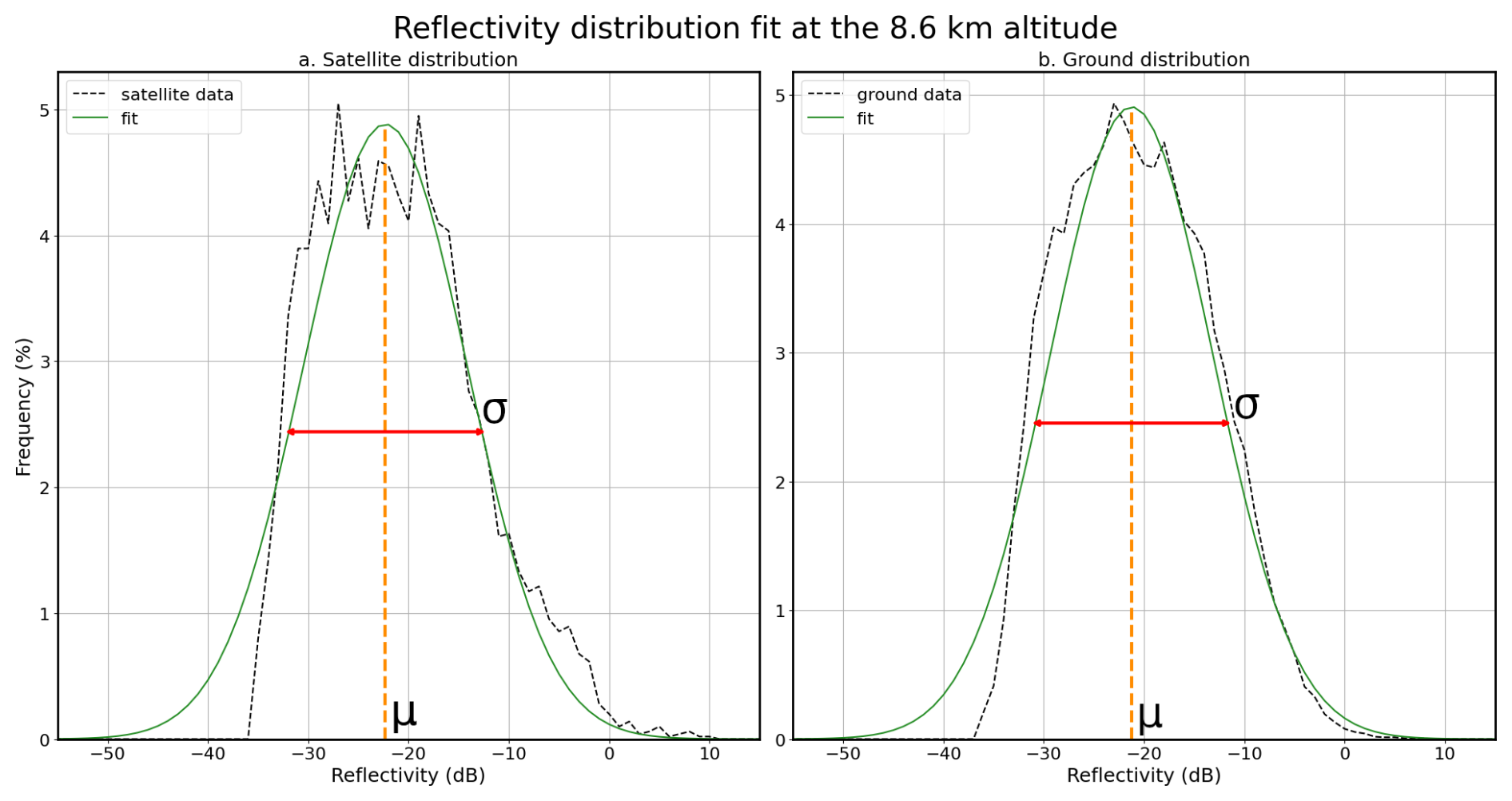
Figure 4 Example of the fit for the distribution of the height bin at 8.6 km height. The left panel shows the fit for the satellite. The right panel shows the fit for the RPG94 of Jülich.

Figure 4 shows an example of the fit of the reflectivity distributions from the height bin of 8.6 km for CPR and ground radar of the Jülich RPG94. From the fit, a fourth R² parameter is evaluated, representing the goodness of the fit.

The fitting of the reflectivity distribution allows us to evaluate the main parameters of the CFADs, dismissing the impact of noise that could exist in the extremum of the distribution. The calculated mean of the distribution and centre (μ) are thus not necessarily coincidental. The centres profiles are then used as an estimator to evaluate the inter-instrument reflectivity bias. We then use 3 parameters from the fit to evaluate the statistical similarity of the reflectivity distribution at each height bin.

The first parameter used is the correlation between the centres. For each height bin, the correlation is calculated considering points ±500 m around the height. This correlation parameter goal is to check that the profiles shapes follow each other. The second parameter used is the weighted ratio between both σ for each height (from now on referred as σ ratio). The σ ratio is given by: $\frac{|{\mathit{\sigma }}_{\mathrm{gro}}-{\mathit{\sigma }}_{\mathrm{sat}}|}{{\mathit{\sigma }}_{\mathrm{sat}}}$. This σ ratio's goal is to check that the width of the distributions are similar for each height bin. The third parameter used is the R² parameter. The R² parameter is evaluated by a linear regression between the data and the fit. The goal of this parameter is to check that the distributions were fitted correctly for each height bin, to be sure that μ and σ were reliably estimated.

The 3 parameters are tested for each height bin, if each of the parameters fulfil a certain threshold criterion the height bin is considered valid for the comparison. The values of these thresholds are the following:

• If the correlation between the centers is larger than 0.9.

• If the σ ratio is lower than 0.4.

• If the R² is larger than 0.85.

The values of these parameters were evaluated through a sensitivity analysis (not shown here), with the following considerations: a high center correlation ensures a high vertical similarity, a low σ ratio indicates a high horizontal similarity and a high R² ensures that the fits accurately represent the data. The three parameters values were then chosen with these considerations, while keeping the highest possible number of selected height bin at the end of the process. The sensitivity test performed showed that tunning the thresholds (corr: ±5 %, $\mathit{\sigma }:\pm \mathrm{25}\mathit{\%}$, $R^{\mathrm{2}}:\pm \mathrm{5}\mathit{\%}$) does not change the final bias. We would however recommend to adapt these parameters if the situation requires it (for example if there is not enough data available for convergence).

For the 35 GHz radars we also check that the ground center reflectivity value is lower than −10 dB. These selection thresholds were verified through sensitivity analyses and the final closure (see Sect. 5).

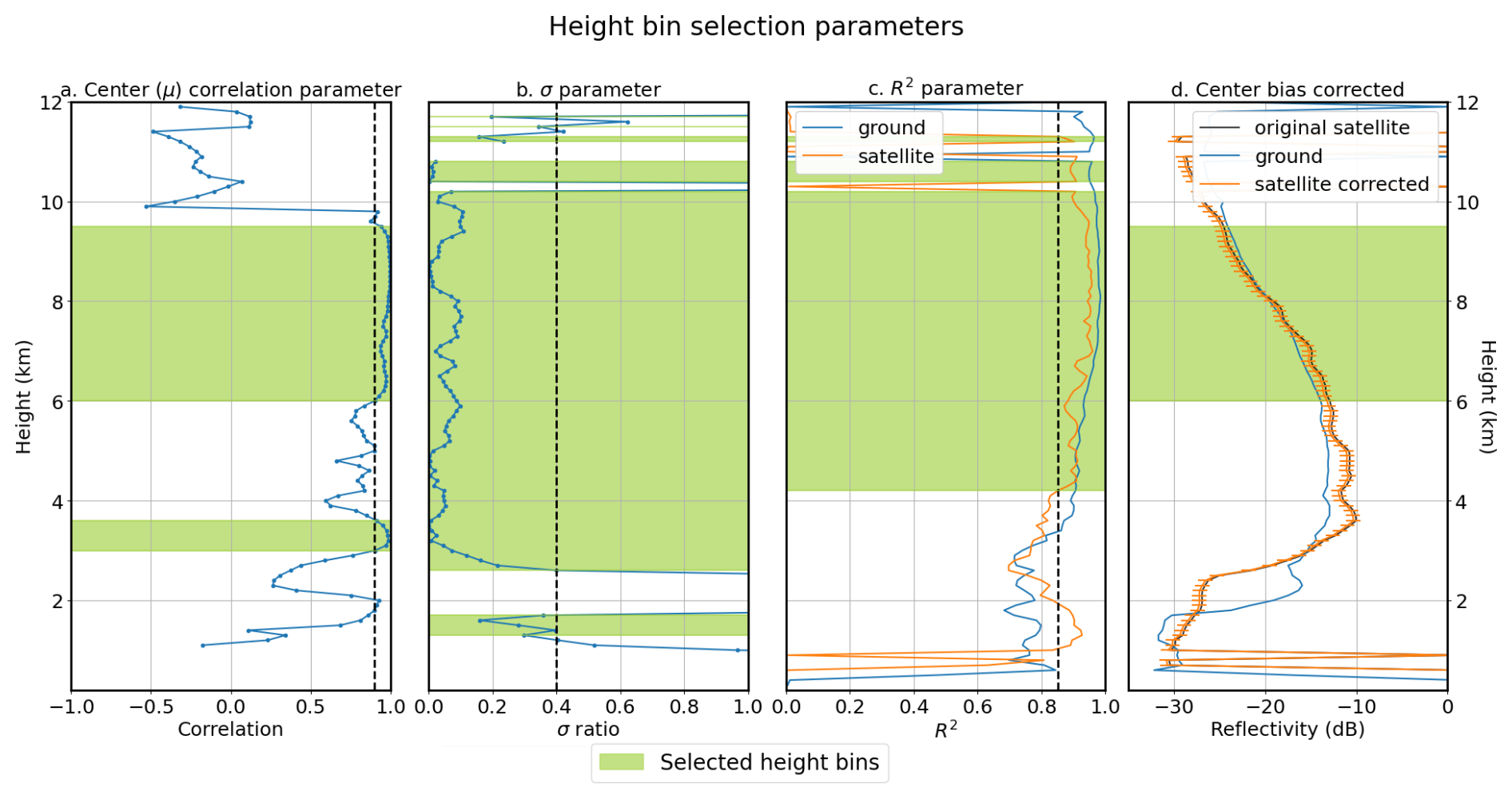
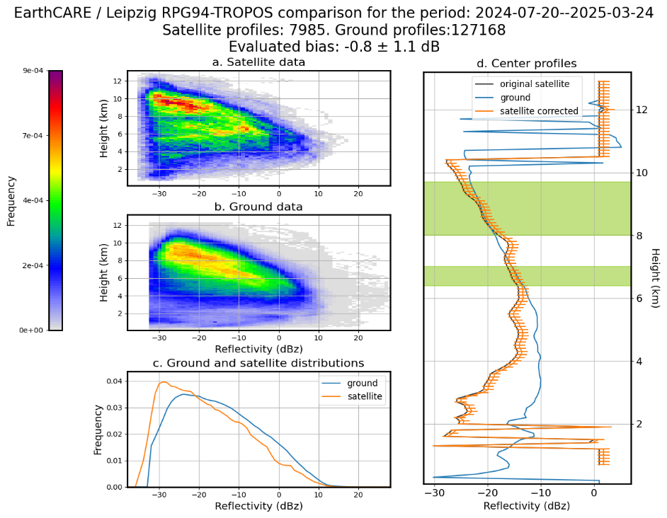
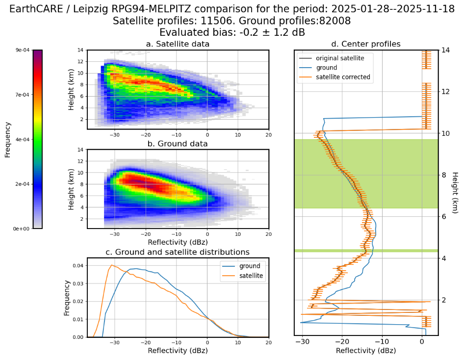
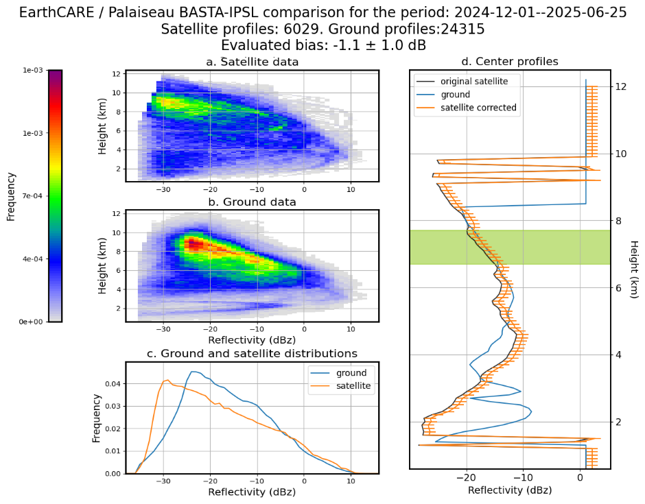
Figure 5 Example of height bin selection and bias estimation for the RPG94 of the Jülich site on a time period from July 2024 to November 2025 (see Table 1). The parameters and center profiles were evaluated from the CFADs presented in panel (3.a.) and (3.b.) of Fig. 3. In panels (a), (b), and (c) the green zone represent the height bin selected for the center correlation, the σ ratio and the R² parameters respectively. Panel (d) shows the ground (blue) and satellite (black) center profiles. The orange profile is the satellite profile corrected for the bias, with its associated uncertainty. The green zone is the height bins selected with the 3 selection parameters.

4.6.3 Bias and uncertainty evaluation

The final satellite-ground bias is estimated as the mean of the centers single bias estimates on the selected bins. The associated uncertainty is then the standard deviation of the centres differences on the selected height. The other sources of uncertainties identified are indicated later in this section. If no height bin is selected, the satellite and ground data are deemed not statistically comparable and thus no bias is evaluated.

Figure 5 shows an example of the height selection process and the inferred bias for the Jülich RPG94. The three first panels a, b and c show the evolution of an individual selection parameter with the altitude. In this figure, the center correlation parameter and R² parameter are the most decisive in the selection of the height bins. The σ parameter seems redundant here discarding only height already discarded by the two other parameters. However, this parameter full fill it's goal to remove height with very different distributions, that could come from different physical observations (ie different cloud statistics, second trip echo). The d panel, shows in green the height zone where all the 3 parameters are full-filled and where the satellite-ground bas is evaluated. This zone is made of 36 height bins, corresponding to a zone of 3.6 km on which the bias is evaluated. The black and blue profiles are the center profiles of the satellite and the ground respectively. For the RPG94 of Jülich these original profiles are very close, showing a small reflectivity bias between the CPR and the ground radar. The bias evaluated for this site is indeed: $Z_{\mathrm{CPR}}-Z_{\mathrm{ground}}=\mathrm{0.3}\pm \mathrm{1.3}$ dB. The orange profile in panel d shows the satellite center profile corrected for this bias with its associated total uncertainty. For each of the radars used in this study a summary figure of the CFADs, reflectivity distributions and the reflectivity center profiles is given in Appendix B.

To evaluate the total uncertainty, we firstly identified 5 sources of uncertainty, from which two are considered and three neglected as explained below.

• σ_GR is the uncertainty on the ground radar measurements. For the calibrated radars used in this study, the measurement uncertainty was estimated during the calibration campaigns (see Table 1). This uncertainty is typically in the range of [0.9; 1] dB.

• σ_B is the standard deviation between the bias estimates at each height bin. It is included as a way to assess the statistical uncertainty inherent to the comparison algorithm. This uncertainty is typically in the range of [0.9; 1] dB.

• σ_C is the uncertainty on the estimation of the centres. As the centres profiles are used for the estimation of the bias, the uncertainty on the centres evaluation needs to be taken into account. This corresponds to the diagonal terms in the covariance matrix for each fit. The total contribution to uncertainty is given by the sum of the uncertainties of the centre estimation for the satellite and the ground ($\mathit{\delta }{c}_{\mathrm{sat}}^{\mathrm{2}};\mathit{\delta }{c}_{\mathrm{gr}}^{\mathrm{2}}$): ${\mathit{\sigma }}_{\mathrm{C}}^{\mathrm{2}}=\frac{\mathrm{1}}{N^{\mathrm{2}}}{\sum }_i\mathit{\delta }{c}_{{\mathrm{sat}}_i}^{\mathrm{2}}+\mathit{\delta }{c}_{{\mathrm{gr}}_i}^{\mathrm{2}}$. This uncertainty is typically inferior to 0.005 dB. This uncertainty source is thus neglected as it is several order of magnitudes less than other uncertainties.

• σ_GA is the uncertainty from the gaseous attenuation. Cloudnet and EarthCARE L2a CPR FMR product provide reflectivity values corrected by attenuation. By assuming that their calculation has no inherent bias, the processing and averaging of large amounts of pixels should average the bias contribution of this term to zero. Thus, we neglect this uncertainty source in the final estimate for the satellite-ground calibration difference.

• σ₃₅ is the uncertainty coming from the comparison of Ka band radar with the CPR. As already mentioned in Sect. 4.6.1, we consider this uncertainty to be negligible when using ground data bellow −10 dB.

The total uncertainty on the bias evaluated σ_t is then given by the equation:

$$\begin{array}{}\text{(3)}& {\mathit{\sigma }}_t=\sqrt{{\mathit{\sigma }}_G^{\mathrm{2}}+{\mathit{\sigma }}_{\mathrm{B}}^{\mathrm{2}}}\end{array}$$

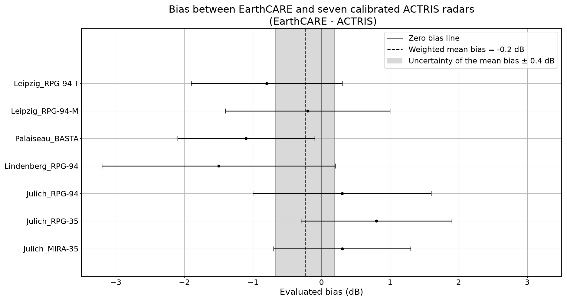
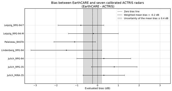
Figure 6 Summary of the biases estimated between EarthCARE CPR and the calibrated ACTRIS ground sites. Each point with its uncertainty represent the bias of between CPR and the respective ground radar. The period used for the bas evaluation are given in Table 1. The grey vertical line at 0 represents EarthCARE, as the biases are evaluated as the difference between EarthCARE and ground reflectivities. The vertical dashed black line is the weighted mean bias of the biases.

5 Validation of EarthCARE reflectivities and of the algorithm with ACTRIS sites

As mentioned in Sect. 3.2 the CCRES component of ACTRIS is performing inter-comparison campaigns using a reference radar moved from site to site. From these campaigns, a correction coefficient is evaluated for the radars of each sites. The radars of the sites of Palaiseau, Jülich, Leipzig and Lindenberg (see Table 1) went through this calibration process. Moreover the ground radars did not go through any changes on the time periods considered.

To validate the algorithm and the CPR reflectivities, we compare the satellite-ground bias estimated for each of these sites, taking account of the calibration correction coefficients. Figure 6 shows a summary of the EarthCARE-ground biases estimated for the radars of the calibrated sites. These biases were evaluated on a time period from 20 July 2024 to 18 November 2025 (or on a smaller time period within), collecting satellite data in a 200 km radius from the site.

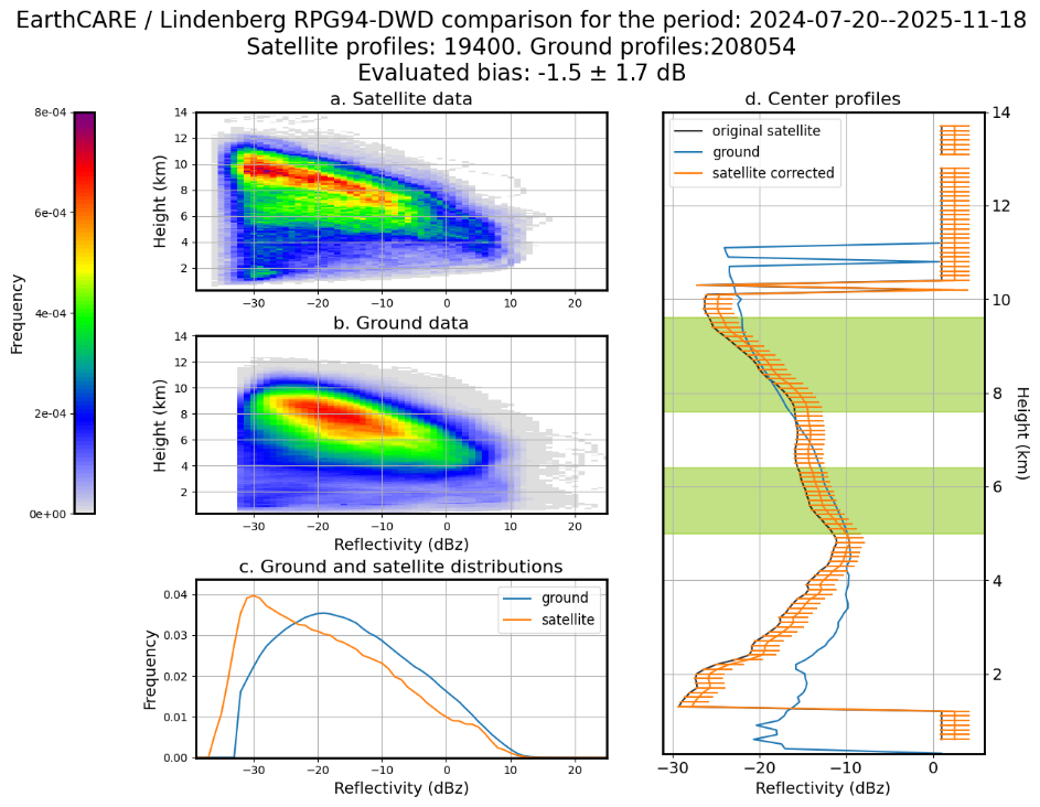
From Fig. 6, we see most individual biases are close to 0 dB. The largest evaluated bias is for the RPG of the Lindenberg site with an evaluated bias of 1.5±1.7. Looking more closely at these results (see Appendix B), the algorithm selects different height zones for the bias estimation. Each of the zone is correct for the bias estimation but they are not coincident, leading to a bias estimate with a higher uncertainty. As the calibration of this radar has been stable and no changes occurred on it during the whole time period, we think that this high bias could come from differences in the clouds observed by both radars. Having more satellite data should help to reduce this uncertainty.

The bias of the radar of Palaiseau is the second largest and only bias for which the uncertainty does not cross the 0 bias line. For this bias, a time period of 6 months was used for the comparison, when at least 9 months was used for the other radars. This observation leads toward the hypothesis that the bias is sensitive to the time period used for its estimation. This hypothesis is explored in more depth in Sect. 6.

Finally, when calculating the mean weighted to uncertainty¹ of all bias estimates we get a likely bias for CPR of $-\mathrm{0.2}\pm \mathrm{0.4}$. This result is consistent with the uncertainty expected from the other calibrations methods. For example, the calibration using the ocean backscatter provides an uncertainty of less than 1 dB and it is currently being used for EarthCARE (Horie et al., 2010, 2025). These biases results validate the calibration of the L2a CPR products. Furthermore, all bias assessments are compatible with the fact that ground-based radars were calibrated using a single calibration source (uniform results within uncertainty), validating the comparison algorithm by closure. BASTA-CCRES, which is the reference radar used as the calibration source for the other ground sites, is calibrated using a reference corner reflector. Hence, ACTRIS calibration value comes from a completely independent source with respect to CPR. This reinforces the reliability of the comparison and of the assessment that EarthCARE L2a CPR FMR product of the BA baseline is unbiased.

6 Time sample impact study using CloudSat and EarthCARE

An important limiting factor for the comparisons is the availability of satellite data. This limitation stems from the fact that some factors like the number of overpasses or the presence of ice clouds during the overpasses cannot be controlled. At present there are no recommendations on the minimum comparisons time (or number of overpasses) needed to obtain reliable bias estimates. To improve the understanding of the impact of the sampling time on the ground-satellite reflectivity comparison, we propose to track the evolution of the bias over a period of time through a time series. We firstly evaluate a bias on the longest time period to act as a baseline. Biases on smaller time periods within the baseline are then evaluated to compare the effects of different time sampling durations on the bias. The following time series focus on the variations of the smaller period biases with respect to the baseline, thus not showing the absolute bias values.

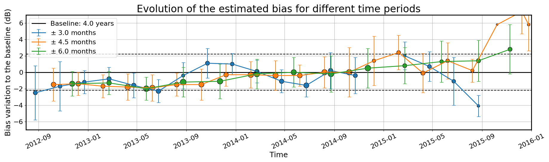
Figure 7 Time series of the evolution of the bias between CloudSat and the MIRA radar of the Lindenberg site between August 2012 and January 2016. The black plain horizontal line represent the baseline bias, with the dotted lines its uncertainty. The blue points are the biases evaluated on a 6 months time period (3 month on each side of the point). The orange points are the biases evaluated on a 9 months time period (4.5 month on each side of the point). The green points are the biases evaluated on a 1 year time period (6 months on each side of the point). The size of the points represent the number of height bin used to evaluate the bias. The largest the point, the more heights were used.

To have a long enough time period to study these effects of time sampling we compared CloudSat reflectivities to the reflectivities from the MIRA radar of the Lindenberg site. Both of the radars were active during a period of less than 4 years spanning from August 2012 to January 2016. As mentioned in Sect. 1, EarthCARE and CloudSat CPRs are overall similar one to the other, with CloudSat CPR being less sensitive. We thus applied our methodology to CloudSat data, using 2B-GEOPROF R05 reflectivity data (CloudSat Project, CIRA, Colorado State University, 2007) and the DARDAR product as a classification to remove profiles with liquid water (Delanoë and Hogan, 2010). Figure 7 shows the CloudSat reflectivities compared with the ground reflectivities of the MIRA radar from the Lindenberg site.

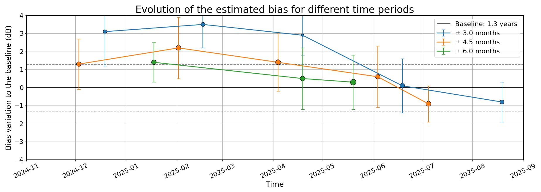
Figure 8 Time series of the evolution of the bias between EarthCARE and the MIRA of the Jülich site between November 2024 and September 2025. The features are the same than for Fig. 7

Looking at Fig. 7, we observe a time changing bias between the two instruments. Previous studies have showed the accuracy of the calibration of CloudSat's CPR (Tanelli et al., 2008). The quality and stability of this calibration was used in later to evaluate the calibration of ground radars (Protat et al., 2009; Kollias et al., 2019). As the time period used here (2012–2016) is in the same time span used by Kollias et al. (2019), we assume that the calibration of CloudSat was stable and that the majority of the CloudSat-ground bias variations come from the ground radar. This assumption is reinforced by the fact that the ground radar has undergone hardware changes during the time period considered. The variability in the bias can be attributed to a misalignment of the phase correction position (PCP) in signal processing chain of the MIRA magnetron. If PCP position is not optimal or drift over time (due to ageing), the misalignment can lead to a suboptimal phase-to-phase correction and consequently in systematic underestimation of the radar reflectivity. The 2 dB bias increase after September of 2013 could be attributed to this effect (Görsdorf, 2026). Another variation in bias is noticeable with the bias for ±4.5 months and ±6 months slowly increasing around January 2015. This indicates that the radar started to reduce it's transmitted power over time. The change in power was noticed by the on site team at the time and decided to change the magnetron and a faulty waveguide in 2016. This indicate that we are able to monitor changes in the calibration from the ground.

Figure 8 shows the comparison of EarthCare data with the MIRA radar from the Jülich site on a period of a little less than a year and a half spanning from 20 July 2024 to 18 November 2025.

Looking at Fig. 8, the biases from the ±4.5 months and ±6 months are mainly within the uncertainty of the baseline. Considering the ±3 months, half of the biases estimated are out of the baseline uncertainty and the algorithm is not able to infer a bias point for October 2024 (each ±3 months points is 2 months apart, hence why the first point on the figure is mid December 2024). The ±3 months time period thus seems less suitable to estimate a solid bias value. However we observe a decrease in the bias estimate for the 3 time periods considered. This phenomena is also observed for the other radars of the Jülich site and could be the consequence of changes in the target observed at this site, as EarthCARE and the ground radars calibration are regularly monitored. Moreover a change in the calibration of the three ground radars at the same time seems unlikely. This variation could indicate a seasonal variability of the estimated bias, however we do not have enough data at the moment to conclude on this variation.

From Figs. 7 and 8, we assess that the minimum time period needed to obtain a solid reflectivity comparison would be ±4.5 months (ie: 9 months time period). This ±4.5 months time period give biases in the uncertainty of the baseline most of the time. The ±3 months (ie: 6 months) time period is much more variable and in some cases does not give enough data to be able to evaluate a bias through our method. In the frame of the monitoring of a ground network, the ±3 months bias could then be used as a preliminary value of the bias to be reinforced with longer time periods. The ±6 months (ie 1 year) time period, seems to be the most precise, showing the less variations to the baseline and always being within the baseline uncertainty. This ±6 months time period, thus seems to be optimal to evaluate a solid bias value. Moreover, both CloudSat and EarthCARE results confirm the capacity of our method to see changes in the calibration of ground radar, and thus the possibility to use it to monitor the calibration of zenith looking ground radars as it is done with CloudSat in Protat et al. (2011).

7 Conclusions

This article presents a new algorithm that enable improved comparisons of calibration between satellite and ground-based cloud radars. The algorithm has been developed to check the reflectivity retrievals of the EarthCARE mission, by using calibrated sites of the European ACTRIS infrastructure. Its operating principle relies on the statistical comparison of vertical ice cloud reflectivity profiles.

To compare, we firstly identify a time period where no hardware or calibration changes have been registered on the ground-based radar. We have set on six months as the shortest period usable for this study. Then, all the ground-based vertical ice-cloud profiles sampled in the period are kept for the next statistical analyses. Similarly, all satellite ice-cloud profiles sampled within 200 km of the ground-site in the same time period are kept. Ice cloud profiles are distinguished from liquid using the target classifications from CloudNET and EarthCARE L2a CPR TC products, for the ground and space-based radars respectively. The satellite and ground reflectivity products also provide corrections for atmospheric gas attenuation.

Ground-based data are resampled to match EarthCARE vertical resolution, enabling to fit both lines of sight at the same height bins with a Gaussian function. The parameters from these fits are then used to select the height bins of most statisticall comparability. The reflectivity bias between EarthCARE and the ground radars is then evaluated at the selected heights. The method takes account of the uncertainty contributions from the statistical comparison, and from the ground-based radar calibration, to provide a calibration bias estimate with an associated uncertainty value.

The algorithm is tested by closure with seven calibrated radars from the ACTRIS network. All seven sites show results compatible with the assertion that they are equally calibrated, providing coherent bias estimates within uncertainty.

On a time period of a year and a half, we infer a mean bias $-\mathrm{0.2}\pm \mathrm{0.4}$ dB between EarthCARE L2a CPR FMR product and the average calibration of the ground-based radars. This estimate with very low uncertainty is achieved with a weighted average of the seven calculated biases. Indeed each individual estimate has an uncertainty of ≈1 to 1.5 dB, highlighting the usefulness of having an homogeneous ground-based network for satellite calibration and validation studies. Due to the lower bias value found with respect to its uncertainty, we can conclude that the L2a EarthCARE CPR FMR product of the BA baseline is well calibrated, providing unbiased reflectivity retrievals.

During the development of this study, it was found that a critical parameter for the reliability of the comparisons is the availability of data for both ground and space radars. This motivated the use of all vertical profiles for ground-sites, and to investigate how the length of the time period affects the bias results. A remarkable conclusion from the first measure is that space and ground data remain comparable even if they are not co-localized in time. This suggests that EarthCARE is indeed capable of sampling typical reflectivity values for a given land surface, opening the door to future research into the climatological applications of its measurements. Ground-based networks such as ACTRIS could be used to validate the methods and results used in such climatological studies.

Regarding the impact of the time period length, from comparisons of ACTRIS with CloudSat and EarthCARE, we conclude that a minimal comparison time period of 9 months is recommended for European latitudes (mid-latitude sites). The time series of EarthCARE bias estimates also indicate a possible seasonal variability of the bias estimate, yet there is not enough data to confirm or reject this hypothesis. Investigations on the relevance and source of this possible variability will be possible when a few years of EarthCARE data is collected.

As future work, it could be interesting to research new ways of reducing the time required to make reliable estimations of the calibration bias. This would benefit the resolution of the bias time series, enabling a quicker detection of calibration changes.

One possible approach could be the use of an optimized radius for each ground-based site. We think that a more fine determination of this parameter could enhance the speed at which comparable data is added to the global statistics used in the comparisons. Radius optimization could be done on a statistical basis, or even for single individual overpasses, depending on cloud homogeneity and dominant winds at each site.

Another point for future research could be the study of the impact of latitude in the comparisons. The latitude of the ground-based site is highly relevant for two reasons: sites on near pole latitudes have more satellite overpasses, in the order of one per day instead of one per week, significantly increasing the rate of data collection. Data collection increase if further amplified by the nature of high latitude sites, which are also more likely to have ice clouds, and less likely to have liquid precipitation when compared with near equator sites. For the same 200 km selection radius for satellite data, we would expect near pole radars to need half or even less sampling durations to obtain as reliable comparisons as what we obtained for the European sites.

Moreover, the use of the EarthCARE synergistic classification (AC-TC) should be investigated when the product will have undergone further validation. It could be used to filter profiles containing supercooled liquid water. This filtering should however be investigated carefully in order to be precise as both ground and satellite lidars have a different geometry of observation.

Overall, we think that for future optimizations of satellite versus ground radar comparisons, it will be necessary to consider the interplay between sampling time, radius for satellite data selection, overpass frequency and the cloud characteristics at the latitude of each site.

To summarize, the validated methodology presented in this article will allow the community to continuously check EarthCARE reflectivities by using the ACTRIS cloud remote sensing network or other similar structures. We also think that the algorithm can be used in both ways, enabling the estimation of ground radar calibration biases by using EarthCARE as the reference. Such application would prove beneficial for remote ground-sites, such as Arctic observatories, or the new AWACA sites deployed in Antarctica (AWACA Project, 2026). Finally, the method can be applied on cloud radar networks in general to monitor their calibration homogeneity and stability, continuing and improving on the developments that started with CloudSat in the past.

Appendix A: Impact of the selection time for the ground data

As stated in Sect. 4.1 previous study selected the ground data in a ± 1 h window around the overpass time. However selecting the data in a window around the overpass time does not guarantee that the ground radar will observe the same clouds as the one observed by the satellite. In most of the cases the ground radar sees different reflectivity statistics than the satellite, by selecting the data in a ± 1 h window around the overpass time. This can be seen in the figures provided in the Supplement, showing all the individual overpasses for the site of Juelich. On the 183 overpasses on the considered time period, only 20 show similar clouds between the ground and satellite. The assumption behind the selection criteria of ± 1 h window around the overpass time is that the satellite and ground statistics will converge and be comparable over time. If the statistics build up over time and eventually become similar, even though for most of the overpasses the satellite and ground do not observe the same clouds, this means that the satellite and ground radar should observe similar reflectivity statistics over time even if their observations are not coincidental in time.

By passing over the site the satellite should sample parts of the ground ice climatology. Assuming that our methodology enables us to select the data at heights at which they are the most statistically similar, we consider that evaluating the bias at these height bins should lead to comparing similar clouds observed by both the satellite and ground. This is our assumption to select all the ice profiles from the ground. As clouds change with seasons and with the diurnal cycle, we also ensure that the data contribution from the satellite and ground is evenly distributed in time.

The difference between these two selection method for the ground data is presented in the two next figures. In these we show the satellite and ground CFADs, reflectivity distributions and center profiles for both ground data selection methods, for the RPG94 radar of the Jülich site. From Fig. A1 we see that selecting data in a ± 1 h window allows to obtain similar satellite and ground profiles. However to infer a bias we lower the center correlation selection parameter to 0.8 instead of 0.9 as described in Sect. 4.6.2. Figure A2 shows the comparison selecting all the ice profiles for the site. Here both satellite and ground profiles are also very similar. Comparing the ground CFADs from both figure, we observe that they exhibit similar features, but the one from Fig. A2 is much more statistically defined. Looking at the number of profiles used to make each CFAD, the selection in a ± 1h window allows to collect a bit less than 7000 profiles when the selection of all the ice profiles form the site select almost 200 000 profiles. Using the same height bin selection parameters, we evaluate a bias of $-\mathrm{0.6}\pm \mathrm{1.2}$ dB selecting the data in a ± 1 h window and a bias of 0.4±1.3 dB selecting all the ice profiles. These two biases are compatible one with the other and we thus think that with more time to collect data, both ground data selection method should converge to the same bias values.

As the results from Sect. 5 validate the algorithm by closure, they also validate selecting all the ground ice profiles for the comparisons with the satellite.

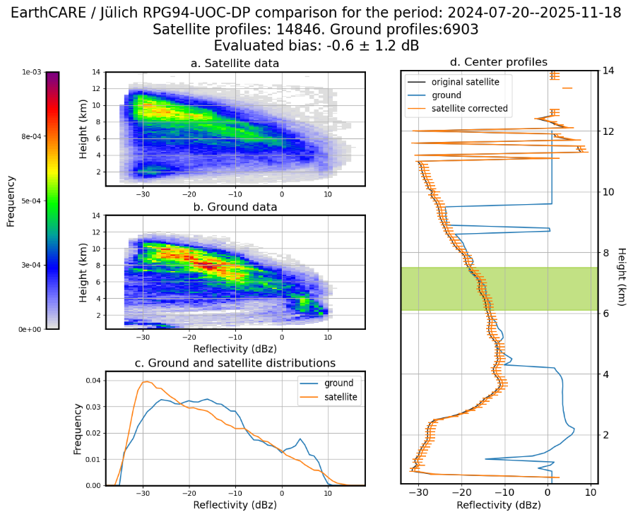
Figure A1 Comparison of EarthCARE with the RPG94 of the Jülich site, by selecting the ground data in a ± 1 h window around the satellite overpass time. The title of figure gives the informations of the time period used and the number of profiles collected for the ground and satellite radars. Panels (a) and (b) show the CFADs of the satellite and ground respectively. Panel (c) shows the reflectivity distributions for both the ground and satellite. The last (d) panel shows the center profiles of the ground, the satellite and the center profile corrected with the evaluated bias and its associated uncertainty.

Figure A2 Comparison of EarthCARE with the RPG94 of the Jülich site, by selecting all of the ground ice profiles in the time period considered. The features of this figure are the same than for Fig. A1.

Appendix B: Detail: Satellite-ground comparisons for each evaluated bias (Fig. 6)

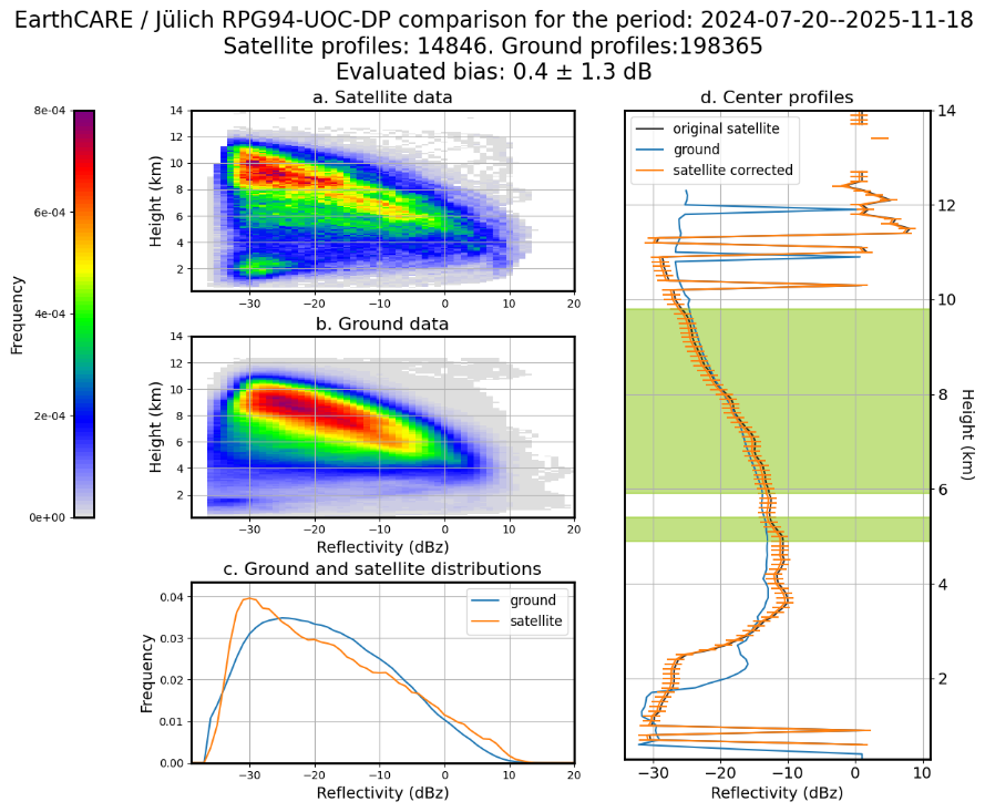
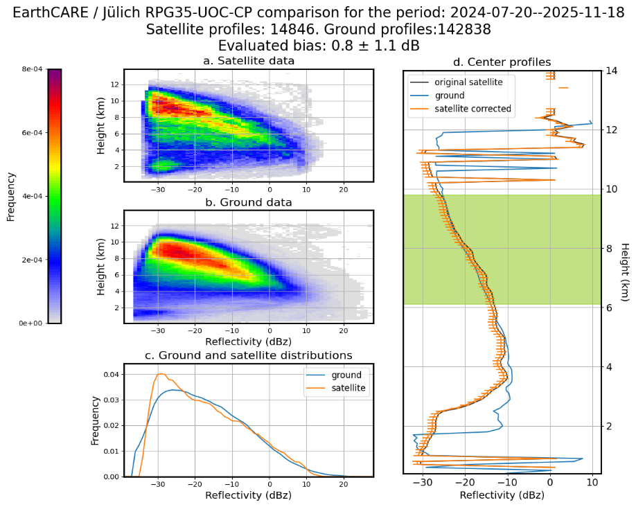
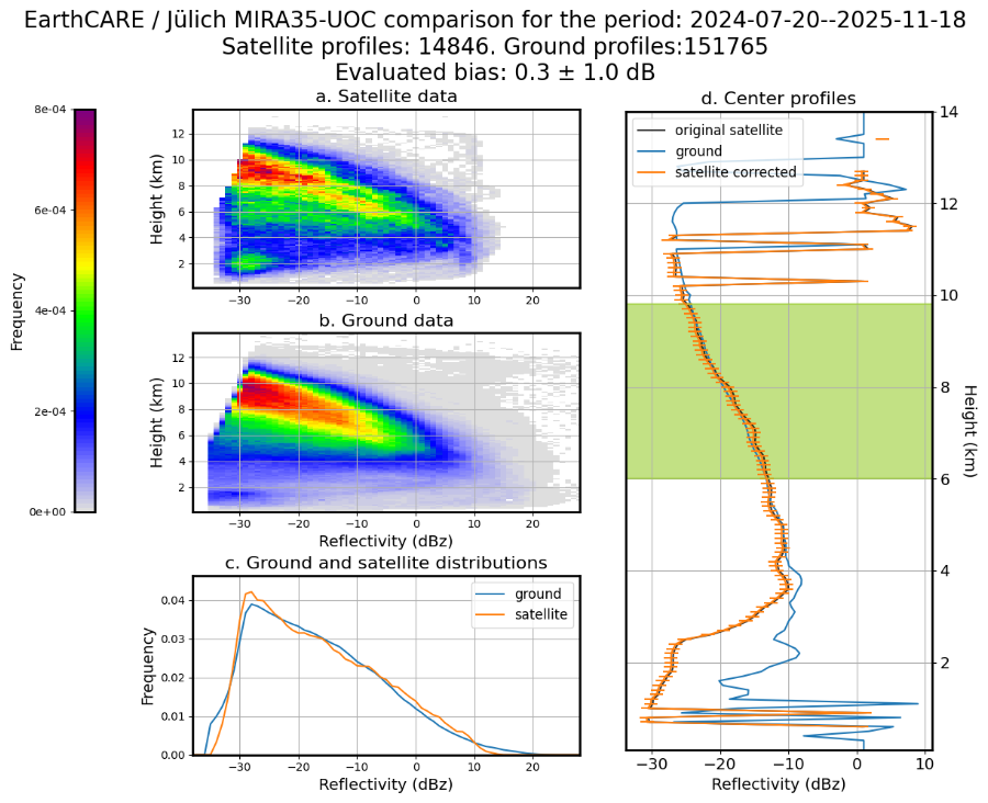
The figures presented in this appendix show details of the comparisons and of the bias evaluation for each radar used in this study. The biases and uncertainty are reported in Fig. 6 as a summary of the EarthCARE-ACTRIS comparisons performed in this study. The figures have 4 panels each. Panels a and b show the CFADs of the satellite and ground respectively. Panel c shows the reflectivity distributions for both the ground and satellite. The last d panel shows the center profiles of the ground, the satellite and the center profile corrected with the evaluated bias and its associated uncertainty. For each figure, the title also gives the time period used, the number of profiles for the satellite and the ground accumulated and the evaluated bias with is uncertainty. The bias is evaluated as described in in Sect. 4.6.

Figure B1 Comparison of EarthCARE with the RPG94 of the Jülich site.

Figure B2 Comparison of EarthCARE with the RPG35 of the Jülich site.

Figure B3 Comparison of EarthCARE with the MIRA35 of the Jülich site.

Figure B4 Comparison of EarthCARE with the RPG94 of the Lindenberg site.

Figure B5 Comparison of EarthCARE with the RPG94 (TROPOS) of the Leipzig site.

Figure B6 Comparison of EarthCARE with the RPG94 (MELPITZ) of the Leipzig site.

Figure B7 Comparison of EarthCARE with the BASTA of the Palaiseau site.