Global variability in the detectability of power plant NO₂ plumes from space

We present the first global, data-driven analysis of power plant NO₂ plume detectability from space. Using TROPOspheric Monitoring Instrument (TROPOMI) observations (nadir pixel size 3.5–7 km) over 6000 of the world's highest-emitting power plants and hourly Continuous Emissions Monitoring Systems (CEMS) data for 500 US plants, we develop an automated algorithm that labels plumes and attributes them to their sources with 98 % accuracy. For the subsequent detectability analysis, we restrict to plants outside interference zones (at least 20 km from other major power plants and 45–90 km from cities (depending on city size)), which retains 45.0 % of US and 21.1 % of global NO_x emissions in our datasets. We then train a machine learning model to predict plume detectability (the probability of detection given the observation conditions) from meteorological, environmental, sensor, and power-plant variables sampled at the single TROPOMI pixel over each plant (F1 score>0.66, AUC>0.8). Out of 25 variables, we find that NO_x emission rate, surface altitude, surface albedo (NO₂ window), sensor zenith angle, primary fuel type, and wind speed jointly explain much of the variability in detectability. For US power plants, an hourly NO_x emission rate of ≈ 400 kg h⁻¹ corresponds to ∼ 50 % detectability, but detectability varies from < 20 % to > 60 % under different combinations of these conditions. These results provide the first empirical quantification of the physical and environmental factors that govern NO₂ plume visibility in TROPOMI data, establishing a foundation for models to use similar predictors as auxiliary variables when quantifying emission rates from plume appearance.

1 Introduction

Fossil-fuel power plants are among the largest emitters of anthropogenic air pollution and greenhouse gases, responsible for approximately 22 % of NO_x and over 40 % of CO₂ emissions globally (McDuffie et al., 2020; Crippa et al., 2022). Accurate quantification of these emissions is essential for enforcing air-quality regulations (U.S. Environmental Protection Agency, 1970; European Commission, 2010) and tracking progress toward international climate goals (UNFCCC, 2015). However, current global emission inventories exhibit substantial spatial and sectoral gaps, particularly in developing and rapidly industrializing regions (Cusworth et al., 2021; Guo et al., 2023; Couture et al., 2024). These gaps stem in part from the limitations of bottom-up accounting, which typically relies on fuel consumption statistics, emission factors, and engineering-based estimates (Guevara et al., 2024). In high-income countries, more robust systems such as Continuous Emissions Monitoring Systems (CEMS), which measure stack-level emissions continuously using instruments like NO_x analyzers, flow meters, and opacity monitors and report hourly averages, enable direct, high-frequency reporting (Ding et al., 2025). In contrast, most power plants in low- and middle-income countries lack such infrastructure, leading to emissions inventories that are often uncertain, inconsistent, or outdated (Srivastava et al., 2024; Cusworth et al., 2021).

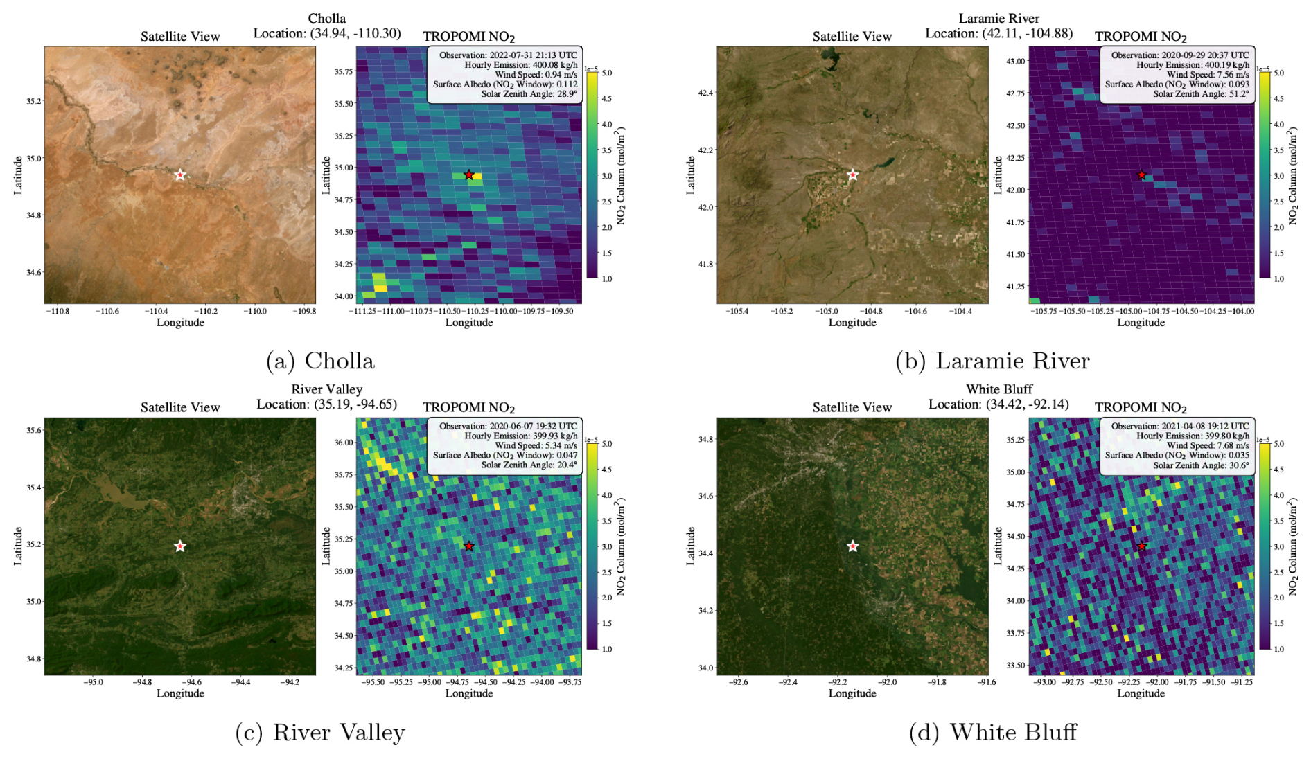
Figure 1 Comparison of tropospheric NO₂ vertical column densities observed by satellite over four US power plants with closely matched hourly emissions (≈ 400 kg h⁻¹). NO₂ plumes are visible near Cholla and Laramie River (top row); no significant enhancement is detected near River Valley or White Bluff (bottom row). The TROPOMI overpass time and observed conditions (100 m wind speed, surface albedo in the NO₂ window, solar zenith angle) are annotated on each panel. Basemap: ArcGIS World Imagery (Powered by Esri) (Esri, 2026) via contextily (Arribas-Bel and contextily contributors, 2024).

Satellite observations offer a top-down alternative for monitoring NO_x emissions at global scale. Early demonstrations with the Ozone Monitoring Instrument (OMI) established wind-rotated downwind-plume methods for extracting emission rate and lifetime, and applied them to tens of major cities and power plants (Beirle et al., 2011; Liu et al., 2016; de Foy et al., 2015). TROPOMI's finer spatial resolution has substantially advanced this line of work: Exponentially-Modified Gaussian (EMG) and related top-down methods have been extended to power plants in North America and beyond (Goldberg et al., 2019; Lange et al., 2022; Tang et al., 2024), and the divergence method has produced global point-source catalogs that now contain over a thousand identified NO_x sources (Beirle et al., 2019, 2021, 2023). These works typically focus on a small number of high-emitting facilities under favorable meteorological and observational conditions, revealing both the potential and limitations of current detection capabilities.

A complementary line of research has focused on plume identification rather than quantification, asking whether a plume is discernible on a given overpass and using automated or learning-based methods to scale detection across many sources. Supervised image classification has been demonstrated for NO₂ on TROPOMI (Finch et al., 2022), while the analogous methane and carbon dioxide literature is more developed, with detection and quantification frameworks for individual plumes and super-emitters across multiple sensors (Kuhlmann et al., 2019; Cusworth et al., 2021, 2023; Lauvaux et al., 2022; Schuit et al., 2023; Rouet-Leduc and Hulbert, 2024; Dumont Le Brazidec et al., 2025; Liu et al., 2020; Bruno et al., 2024). Theoretical expectations for plume column behavior are well established: for a steady point source, the downwind column enhancement scales linearly with the emission rate and inversely with the product of wind speed and the horizontal spread of the plume (Varon et al., 2018), while the effective NO_x lifetime is modulated by photolysis, the OH concentration, and temperature (Valin et al., 2013; Romer et al., 2018; Laughner and Cohen, 2019). On the retrieval side, sensitivity depends on air-mass factor (AMF) geometry, surface and cloud conditions, and background noise (Palmer et al., 2001; Boersma et al., 2011; Eskes and Boersma, 2003; Lorente et al., 2017; Verhoelst et al., 2021). To date, no published work has systematically studied power plant plume detectability at the global scale, nor modeled when and why plumes become observable in TROPOMI data.

Amidst the current satellite-based efforts to monitor anthropogenic NO_x emissions, a challenge persists: power plant plumes with similar NO_x emissions exhibit vastly different detectability (the probability of detection given the observation conditions) across regions, as illustrated in Fig. 1. This variability is driven by meteorology, surface albedo (NO₂ window), sensor geometry, and interference from nearby sources. While previous studies have demonstrated TROPOMI's detection feasibility for individual power plants (Tang et al., 2024) and characterized plume detectability for individual ships (Kurchaba et al., 2024), they have not systematically characterized the conditions that enable or inhibit detection across thousands of power plants globally. We address this scalability gap by asking: what meteorological, environmental, power plant, and sensor geometry variables determine whether a plume of given emission strength will be detectable? Answers to this question have implications for improving satellite-based NO_x inverse modeling as well as future sensor design.

Specifically, we aim to systematically explain the spatiotemporal variability of NO₂ plume detectability from power plants using satellite observations. To do so, we develop a machine learning pipeline that first labels NO₂ plumes in TROPOMI (Sentinel-5P) images and then predicts plume detectability using features including meteorology, sensor geometry, environment, and power-plant variables. We apply this framework to two datasets: (1) US power plants with hourly CEMS data and (2) global high-emitting power plants using a 2018 annual NO_x inventory.

Our contributions are as follows.

1. We present a plume-detection algorithm that achieves 98 % accuracy against manual annotations, designed for point source NO₂ attribution.

2. We produce the first global maps of plume detectability across more than 1000 power plants worldwide, revealing strong geographic patterns. For US power plants, we find that an hourly emission rate of ≈ 400 kg h⁻¹ corresponds to ∼ 50 % detectability, although detectability varies widely depending on location, sensing conditions, and meteorology.

3. We quantify how meteorological, environmental, sensor, and power-plant features influence NO₂ plume detectability across both regional and global scales. Using Permutation Score and SHapley Additive exPlanations (SHAP) Score Estimation, we identify NO_x Emission, Surface Altitude, Surface Albedo (NO₂ Window), Sensor Zenith Angle, Primary Fuel Type, and Wind Speed as the dominant features that govern plume detectability.

Together, these results clarify the observational limits of current satellite NO₂ sensors and provide empirical relationships that can inform future satellite-based emission quantification.

2 Datasets

Our analysis combines five input data sources: Sentinel-5P TROPOMI Level-2 NO₂ retrievals (Veefkind et al., 2012; Van Geffen et al., 2020), which provide both the satellite NO₂ observations and a set of sensor- and scene-level variables (e.g., sensor zenith angle, surface albedo, cloud fraction); U.S. EPA Clean Air Markets Program Data (CAMPD) records (U.S. Environmental Protection Agency, 2023) for hourly NO_x emissions at 500 US power plants; the CoCO₂ global power-plant emission catalog (Guevara et al., 2024) for annual NO_x emissions at 6000 plants worldwide; European Centre for Medium-Range Weather Forecasts (ECMWF) ERA5 reanalysis (Hersbach et al., 2020) for meteorological variables; and the SimpleMaps World Cities Database (SimpleMaps, 2025) for the locations and populations of nearby urban areas used in the interference filter. The subsections below describe each source and the resulting feature set.

2.1 Satellite NO₂ Measurements

To form the observation dataset, we used satellite data of tropospheric NO₂ vertical column densities (Van Geffen et al., 2020) from the TROPOMI instrument aboard the European Space Agency's (ESA) Copernicus Sentinel-5P satellite (Veefkind et al., 2012). Launched in October 2017, TROPOMI provides data at a nadir spatial resolution of 3.5 km (across-track) × 7 km (along-track), which improved to 3.5 km × 5.5 km in August 2019; pixel size increases toward the swath edges due to viewing geometry.

We downloaded raw Level-2 NO₂ data in NetCDF format from the NASA Earthdata portal. Each file corresponds to a single satellite orbit (∼ 101 min), containing one Level-2 swath with 450 across-track ground pixels and thousands of along-track scanlines. For our US analysis (1 January 2019–31 December 2024), we acquired 9636 files. For the global analysis (1 May–31 December 2018), we obtained 3421 files. The data come from the v2 series of the TROPOMI L2 NO₂ processor (v2.4.0–v2.8.0), spanning both the reprocessed (RPRO) and operational offline (OFFL) streams. The May 2018 start of the global window is set by the v2.4.0 NO₂ full-mission reprocessing, which begins on 1 May 2018; earlier observations are only available in the v1 product line, which is not directly comparable.

Throughout this paper we use observation to refer to one TROPOMI overpass at a target power plant: the L2 NO₂ retrieval at the pixel closest to the plant's center, paired with the corresponding emission record.

To generate a high-quality dataset, we processed these raw files through a multi-step filtering pipeline. For each TROPOMI observation over a power plant, the observation is kept if it contains:

1. a quality flag greater than 0.75, which removes data contaminated by clouds or other errors (Van Geffen et al., 2022),

2. at least 50 % valid pixels within a 50 km radius of a power plant, and

3. a valid nearest-neighbor pixel over a power plant.

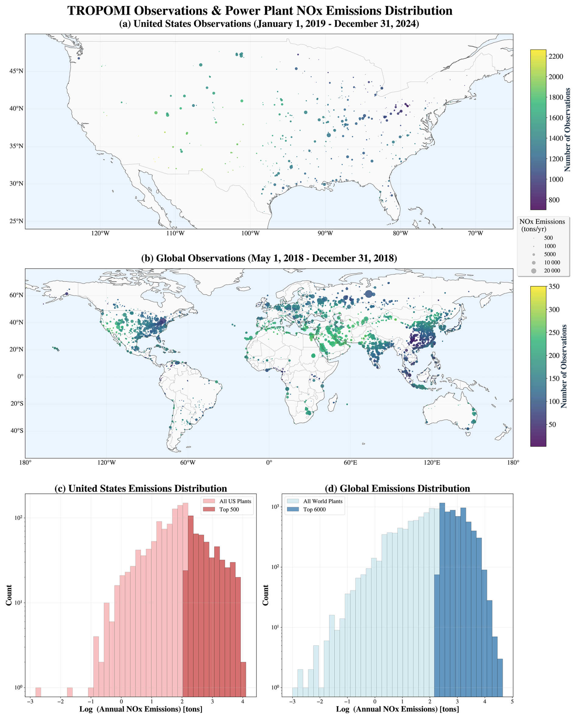
Figure 2 Distribution of TROPOMI observations and power plant NO_x emissions. Panels (a) and (b) show spatial distribution of power plant NO_x emissions (marker size) overlaid with TROPOMI observation frequency (marker color) for the United States and global facilities, respectively. Panels (c) and (d) display emission distribution histograms on a log scale showing all plants (light colors) versus analysis subsets of top emitters (dark colors) for the United States (top 500 plants) and global (top 6000 plants). TROPOMI observation periods: US data from January 2019 to December 2024, global data from May to December 2018. Dataset: full quality-filtered dataset (n=666 222 US and n=875 686 global TROPOMI observations).

After applying these quality assurance criteria, this process yielded a final dataset of 666 222 high-quality observations for the US analysis and 875 686 for the global analysis. Across the mapped facilities (US, N=500; global, N=6000), observation coverage is extensive. In the US, plants have a median of 1301 observations (10th and 90th percentiles of the per-plant distribution P₁₀=1050 and P₉₀=1645; we use P_X to denote the Xth percentile of whichever per-plant distribution is under discussion, applied throughout to observation counts, detection counts, and detectability values). Globally, the median is 141 observations (P₁₀=90, P₉₀=218), with 98.8 % of plants having ≥ 50 observations (range 2–350). As illustrated in Fig. 2a and b, the geographic density of these final observations is highest in drier, less cloudy regions and at higher latitudes.

2.2 Hourly NO_x Emissions in the US

CAMPD, maintained by the U.S. Environmental Protection Agency (EPA), provides hourly emissions data for CO₂, NO_x, SO₂, and mercury from individual power plants. This level of granularity is unique globally and offers a distinct opportunity to study how emission rates influence the detectability of NO₂ plumes in satellite imagery. For our analysis, we downloaded hourly NO_x emission data from the CAMPD API, specifically matching the times of TROPOMI satellite observations for each plant.

CEMS provide these hourly emissions data by measuring pollutant concentrations and exhaust flow rates to compute mass emission rates. These systems operate continuously, reporting hourly averaged data directly to the EPA.

The CAMPD inventory is comprehensive, containing 97.1 % of annual US power-sector NO_x emissions as of 2023 (U.S. Environmental Protection Agency, 2023). From this inventory, we selected the 500 power plants with the largest total NO_x emissions from 2019 to 2024, representing the upper tail of all US facilities, for our study; their emission distribution is shown in Fig. 2c. Our selection accounts for 93.6 % of the inventory's NO_x emissions and 79.8 % of its CO₂ emissions. By 2024, 461 of the 500 plants still reported to CAMPD, the remaining 39 having ceased reporting. Among the 461, pipeline natural gas facilities (238 plants, 52 %) and coal plants (176 plants, 38 %) dominated, followed by natural gas (13), wood (12), coal refuse (5), diesel oil (3), other gas (3), process gas (3), residual oil (2), petroleum coke (1), and one plant reporting a combined coal/natural gas primary fuel; fuel type was unreported for a further 4 plants. Over this 6-year period, this group of top emitters transitioned measurably from coal to natural gas: coal-fired plants fell from 229 to 176 (a 23.1 % decrease), while pipeline natural gas facilities grew from 225 to 238 (a 5.8 % increase). For context, the EPA's broader power sector data covered approximately 96 % of US fossil fuel-based electricity generation as of 2018 (U.S. Environmental Protection Agency, Clean Air Markets Division, 2022).

2.3 Annual NO_x Emissions for Global Power Plants

Because global hourly emissions are unavailable, we used annual emissions. For our global analysis, we sourced annual power plant emissions from the CoCO₂ catalog (Guevara et al., 2024). This inventory covers at least 95.9 % of total reported global power plant emissions and provides annual data for CO₂, NO_x, SO_x, CO, and CH₄. The CoCO₂ catalog derived the annual emissions using a bottom-up methodology as follows:

1. Europe: Use each plant's official reported NO_x from the European Pollutant Release and Transfer Register (E-PRTR) and the Large Combustion Plants (LCP) dataset (European Environment Agency, 2020, 2019) for the year. If a plant didn't report, estimate it from other official datasets or standard country-and-fuel ratios.

2. United States: Use the EPA's Emissions & Generation Resource Integrated Database (eGRID; largely CEMS-based) (U.S. Environmental Protection Agency, 2020).

3. Rest of world: Start from national fuel use, convert to NO_x with country- and fuel-specific ratios, then apportion to plants by installed capacity.

These derived annual emissions provide robust annual magnitudes but do not resolve within-year variability. Plume detectability is determined at the moment of each observation; relying on annual emissions therefore limits our ability to predict per-observation detectability.

From this catalog, we selected the 6000 facilities with the largest annual NO_x emissions in 2018, with emissions ranging from 219 to 44 548 t yr⁻¹, representing the upper tail of global power plant emissions; their emission distribution is shown in Fig. 2d. This selection accounts for 96.1 % of the inventory's NO_x and 91.5 % of its CO₂ emissions, and corresponds to at least 92.1 % of global power plant NO_x and 87.7 % of global power plant CO₂ emissions. Coal (3023), natural gas (1810), and oil (690) plants dominate the set, which also includes facilities that burn biomass (354) and waste (123).

To avoid double-counting in our source-attribution analysis, we filtered the catalog for duplicate entries (defined as plants within 3 km sharing identical reported emissions across all five pollutants: CO₂, NO_x, SO_x, CO, and CH₄). This step removed 3320 of 16 461 candidate facilities (20 % of the catalog), with the bulk of removals concentrated in China and India (66 % combined); per-country statistics and a brief discussion of the underlying catalog-integration causes are provided in Sect. S2 in the Supplement.

Table 1 Input features for the plume detectability model by category (Sensor, Power Plant, Meteorology, Environment) and source (TROPOMI, ERA5, U.S. EPA, and Global Inventory).

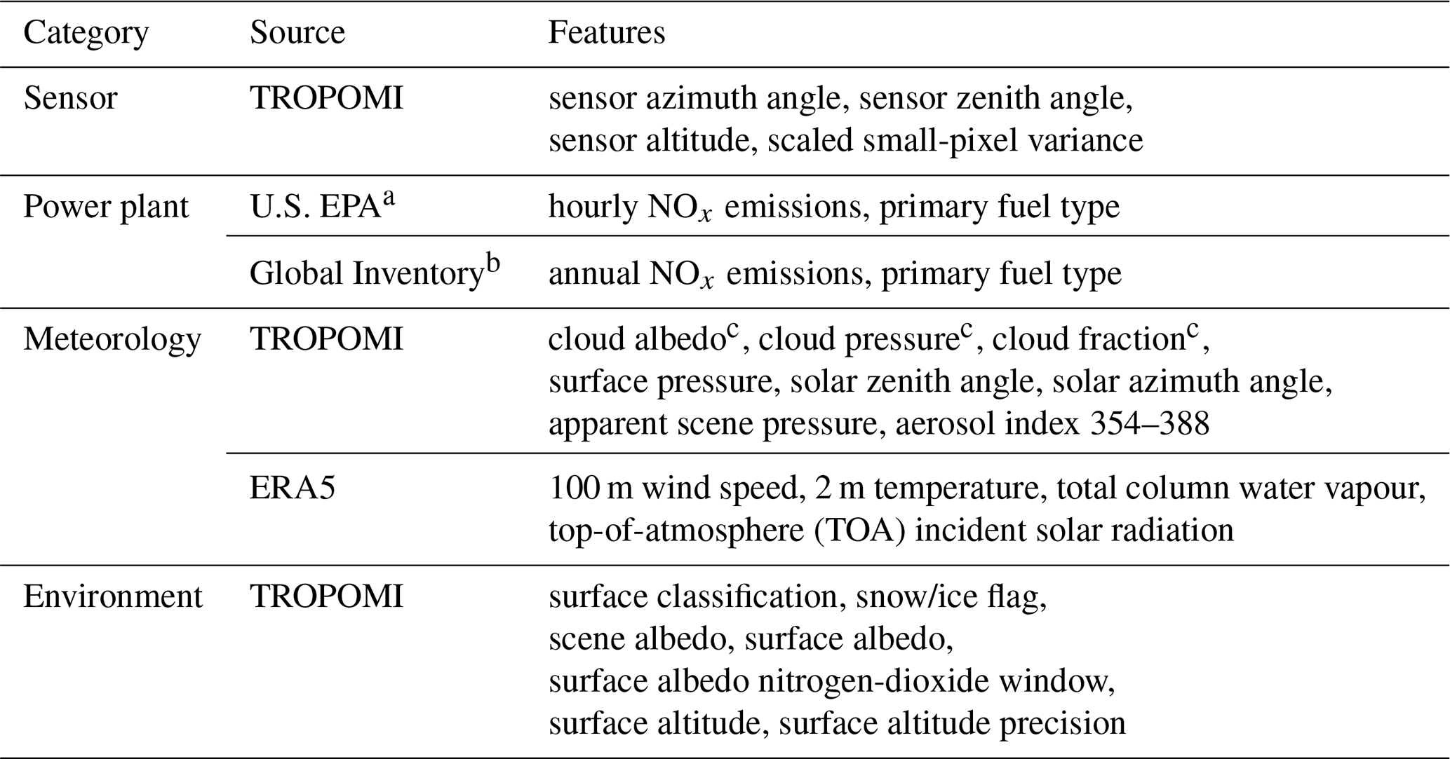
^a Data source for the US analysis. ^b Data source for the global analysis (Guevara et al., 2024). ^c Cloud-product variables provided by the FRESCO (Fast REtrieval Scheme for Clouds from the Oxygen A-band) cloud retrieval, which models clouds as Lambertian reflectors under the Clouds-as-Reflecting-Boundaries (CRB) approximation.

2.4 Features Predictive of Plume Detectability

Table 1 lists the features we selected to predict plume detectability, based on the physical processes that govern plume formation, transport, and satellite detection. These features fall into four categories: sensor characteristics, power plant attributes, meteorological conditions, and environmental context. The variables in these categories capture the complex interplay between emission sources, atmospheric conditions, and observation geometry that strongly influences plume detectability. Several variables labeled as “TROPOMI” in Table 1 are not direct sensor measurements but auxiliary fields packaged into the Level-2 NO₂ product from external datasets (e.g., surface albedo and surface pressure).

We extracted these variables from their respective data sources using several methods:

1. TROPOMI features were extracted from the pixel closest to each power plant's center.

2. ERA5 meteorological fields were matched to each TROPOMI overpass using nearest-neighbor interpolation in both space (to the plant location) and time (to the overpass timestamp).

3. Emission data from EPA or global inventories were used directly.

We describe the variables and their source datasets in Table 1, organized by category.

2.4.1 Sensor

Sensor zenith and azimuth angles, i.e., the viewing zenith angle (VZA) and viewing azimuth angle from the TROPOMI L2 product, define the viewing geometry and optical path length. Along with solar angles and scene albedo, they control the amount of backscattered light available for absorption spectroscopy. The VZA also sets the across-track ground-pixel footprint, which grows from ∼ 3.5 km at nadir to up to ∼ 14 km at the swath edge (Van Geffen et al., 2020), and is itself a likely driver of plume detectability. Sensor altitude varies only modestly along Sentinel-5P's near-circular sun-synchronous orbit (≲ 2 % of the mean in our data), so its direct effect on ground-pixel size and swath geometry is small; it is closely related to latitude and primarily serves as a latitude/orbit-geometry proxy alongside the explicit solar and viewing angles. The scaled small-pixel variance measures sub-pixel heterogeneity that can indicate a plume's presence. Together, these variables establish the instrument's sensitivity to narrow, high-contrast plumes.

2.4.2 Power plant

We include the primary fuel type and emission rate for each power plant. For US facilities, we use hourly emissions; for global facilities, we use annual emissions. The primary fuel type (e.g., coal, natural gas) influences combustion temperature and stack gas buoyancy, which affect plume rise and dispersion. Because higher emissions produce more concentrated and easily detected plumes, emission magnitude is a key predictor of detectability.

2.4.3 Meteorology

We include meteorological variables to account for their influence on plume transport, optical interference, and radiative transfer.

• Transport and Mixing: Wind speed drives horizontal advection and dilution. Temperature influences boundary layer dynamics and vertical mixing, which together determine a plume's rise and spread. We use the 100 m wind speed derived from the ERA5 horizontal wind components (u,v) as a single feature.

• Optical Interference: Cloud properties (fraction, pressure, and albedo) can obscure plumes or create false signals. The TROPOMI 354–388 nm ultraviolet (UV) aerosol index captures absorbing aerosols (e.g., dust, smoke, volcanic ash), which are an important aerosol-related interference in NO₂ retrievals; aerosol optical depth (AOD), which captures total aerosol loading (both absorbing and non-absorbing, including sulfate, nitrate, and sea salt), is not provided by the TROPOMI L2 NO₂ product and is not included in the present analysis.

• Radiative Transfer and Photochemistry: Solar geometry (zenith and azimuth angles) determines the photon path length, while scene pressure and surface pressure define the effective reflecting altitude and total depth of the atmospheric column. Solar zenith angle also affects the actinic flux, which is key in photochemistry: it directly drives NO₂ photolysis, and photochemistry in turn affects the levels of O₃ (which converts NO into the NO₂ that TROPOMI observes) and OH (a sink of NO₂). Total column water vapor affects NO₂ spectral signatures. The TOA incident solar radiation is the downward shortwave solar flux incident at the top of the atmosphere; it is strongly correlated with the solar zenith angle and primarily encodes the joint dependence on latitude and day-of-year.

2.4.4 Environment

We include environmental variables to characterize surface properties.

• Surface Properties: Surface characteristics affect the accuracy of NO₂ retrieval. We use surface classification and snow/ice flags to account for reflectance patterns and potential spectral interferences. We also use surface altitude to establish the vertical column depth. Finally, three albedo features describe surface reflectivity at different wavelengths. Two are at 758 nm, the wavelength of the oxygen A-band used by the FRESCO cloud retrieval: a surface albedo (taken from the TROPOMI Directional Lambertian Equivalent Reflectivity (DLER) climatology of Tilstra et al. (2024) and used as input to FRESCO) and a scene albedo (the effective Lambertian reflectivity of the scene treated as a single uniform reflector). The third is a surface albedo evaluated at 440 nm and applied across the NO₂ fitting window (405–465 nm) for both the cloud fraction retrieval at this wavelength and the air-mass factor calculation.

3 Methods

In this section, we describe our methodology for quantifying the factors that control the detectability of NO₂ plumes in satellite observations. Our systematic approach determines when power plant emissions can be detected from space, and these results help understand the capabilities and limitations of current satellite monitoring.

Throughout this work we distinguish three related quantities that are easily conflated:

• Detection: a binary label produced by the Automated Plume Detection algorithm (Sect. 3.2) for a single TROPOMI observation: 1 if a statistically significant NO₂ enhancement is attributable to the target power plant in the downwind sector, 0 otherwise.

• Detectability: the probability of detection P(detect∣x) given a feature vector x that characterizes the observation conditions, abbreviated P(detect) when context is clear. Detectability is estimated either empirically (as the per-plant ratio of detections to the number of valid TROPOMI overpasses, thereby normalizing out differences in overpass count across plants; Sect. 4.2) or via a machine learning model trained on the binary detection labels (Sect. 3.4).

• Detection frequency: the absolute per-plant count of detections over an observation period (e.g., number of detections per year).

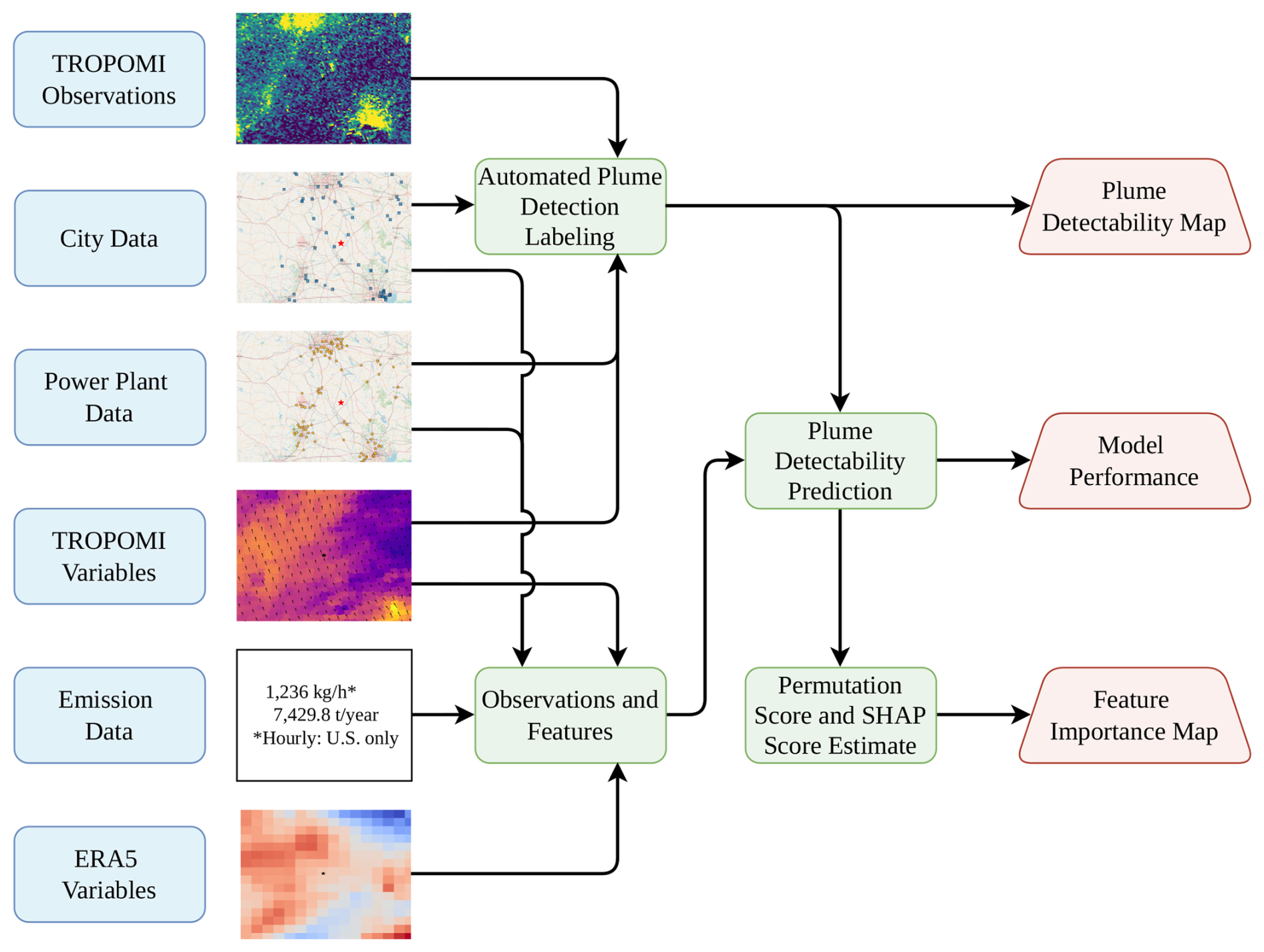
Figure 3 Overview of the analytical pipeline. The process uses input data (blue) to feed the main pipeline processes (green). First, the Automated Plume Detection algorithm produces binary detection labels for each observation. These labels, combined with extracted features, are then used to train a predictive model (Plume Detectability Prediction). In a final step, this trained model is analyzed using permutation and SHAP scores to estimate the importance of each feature (Permutation Score and SHAP Score Estimation). The final products (red) originate from these distinct stages: the detection algorithm generates a plume detectability map, the predictive model's outputs are used for a performance evaluation, and the final analysis generates the quantification of feature importance.

As illustrated in Fig. 3, our analytical workflow consists of four main stages. First, we filter TROPOMI NO₂ observations and extract meteorological and environmental features. Second, we apply our Automated Plume Detection Algorithm to identify detectable plumes in each satellite overpass. Third, we train machine learning models to predict plume detectability from extracted features. Finally, we use the trained models to quantify the relative importance of each feature.

We implement this pipeline in two complementary analyses:

US Analysis: Uses hourly NO_x emission data (2019–2024) from 500 high-emitting power plants with CEMS. For ablations using annual emissions, we use CAMPD's annual NO_x totals downloaded from the same database.

Global Analysis: Uses annual NO_x emission inventories (2018) for 6000 high-emitting power plants worldwide.

3.1 Pairing TROPOMI Observations with Emissions

For each analysis, we pair every TROPOMI overpass over a selected power plant with the corresponding emission record to form the input observations used by all subsequent steps. The TROPOMI-derived input features for the model are extracted from the single pixel closest to the plant's center, not aggregated across the plume.

US. The US analysis uses 666 222 TROPOMI overpasses across our 500 selected plants. This full set of observations is used throughout the manuscript for dataset characterization and detection statistics. For the model training and feature-importance analyses (Sects. 3.4 and 3.5), we use 189 713 observations from 171 plants, namely the subset of overpasses that have (i) no missing (NaN) values in any input feature, since TROPOMI retrieval variables can themselves contain NaNs, (ii) a paired hourly NO_x record from the CAMPD database, and (iii) a target plant lying outside interference zones (Sect. 3.3). CAMPD only catalogs regulated facilities during operating hours with valid CEMS data, so overpasses during monitoring downtime, plant shutdowns, or over facilities below reporting thresholds are excluded.

Global. The global analysis uses 875 686 TROPOMI overpasses across our 6000 selected plants. As with the US dataset, this full set of observations is used throughout the manuscript for dataset characterization and detection statistics; for the model training and feature-importance analyses (Sects. 3.4 and 3.5), we use 161 118 observations from 1065 plants, namely the subset of overpasses with no missing (NaN) values in any input feature, a valid annual NO_x record in the CoCO₂ catalog, and a target plant lying outside interference zones (Sect. 3.3).

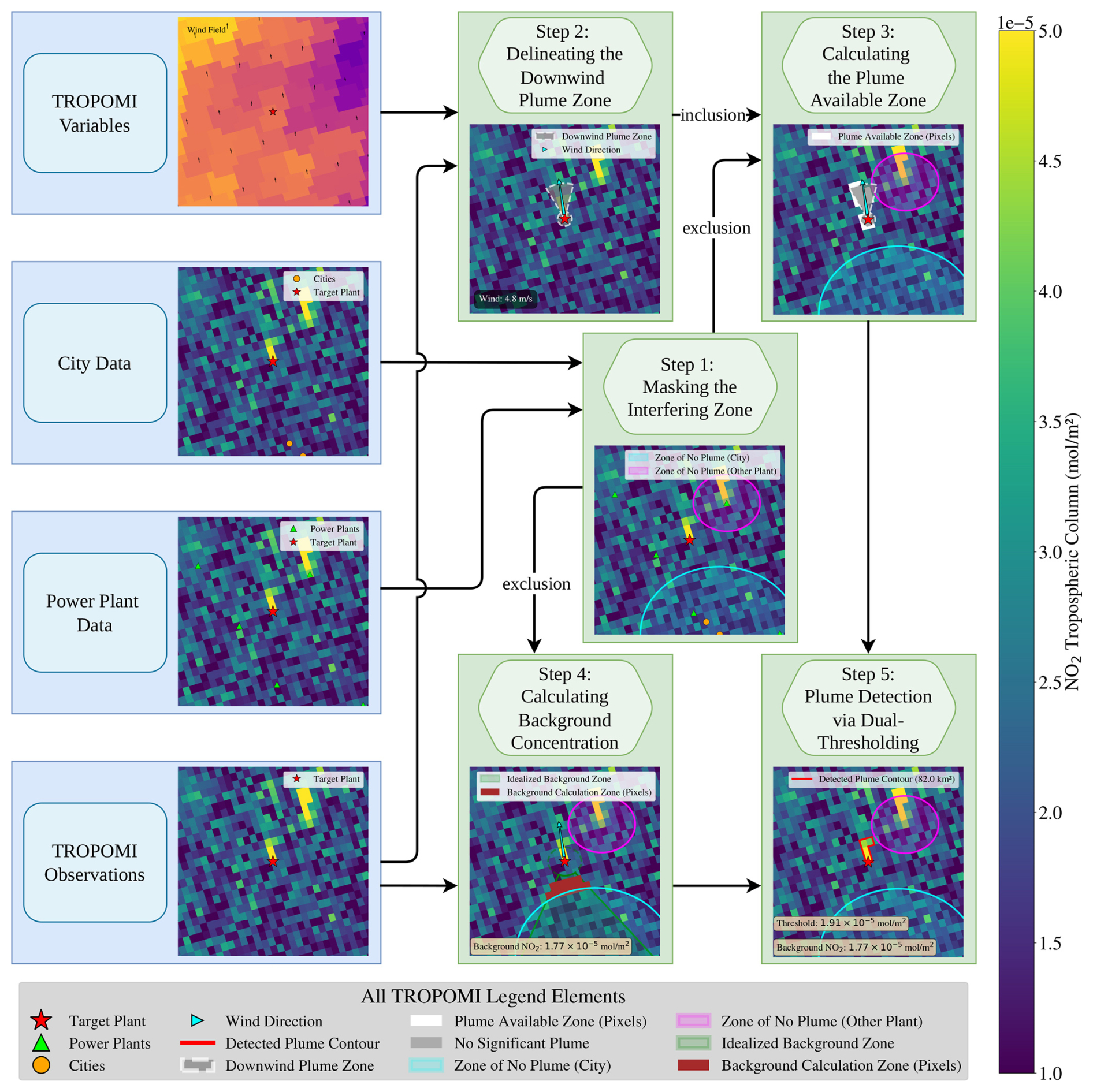
Figure 4 Overview of the Automated Plume Detection Algorithm. The process begins by masking potential interference from nearby cities and power plants (Step 1). It then uses wind direction to define a downwind search area and isolates a “Plume Available Zone” by removing the masked regions (Steps 2–3). Finally, the algorithm applies a dual-thresholding method against the calculated background concentration within the Background Calculation Zone to detect and label the plume (Steps 4–5). Blue boxes represent input data, and green boxes represent algorithm components. A full legend and color bar are provided.

3.2 Automated Plume Detection

To build a machine learning model to explain plume detectability, we first need a large labeled dataset of plume detection. Manual plume annotation is prohibitively costly and inconsistent, so labels must be generated automatically. Existing automated methods such as the Data-Driven Emission Quantification (DDEQ) toolkit (Kuhlmann et al., 2024) detect NO₂ anomalies but cannot attribute a plume to a specific source, failing to separate a target power plant from nearby cities or other industries. To fill this attribution gap, we develop a new plume-detection–with-attribution algorithm that automatically labels plumes and assigns each one to its originating power plant.

Our algorithm automates this attribution through a five-step workflow, outlined in Fig. 4. The process integrates TROPOMI satellite measurements with power plant and city databases to systematically isolate and label a target plume. While the steps are executed sequentially, the figure illustrates the key data dependencies that connect the different stages of the process.

3.2.1 Hyper-parameter Tuning

The tuned hyper-parameters of the Automated Plume Detection Algorithm are: in Step 1, the city population threshold, the plant emission-ratio threshold, the City Masking radius, and the Power Plant Masking radius; in Step 2, the wind-direction tolerance, the maximum search distance, the close-range distance, and the minimum plume area; in Step 4, the upwind sector angle and the background annulus; and in Step 5, the Statistical Significance (2σ) and Absolute Minimum thresholds. Their final values are reported in the corresponding step descriptions below. To tune them, we drew a tuning set of 200 observations: 100 from the global dataset, stratified across six continents and five emission-level quantiles (0 %–20 %, 20 %–40 %, …, 80 %–100 %) with roughly 3–4 observations per (continent, quantile) cell; and 100 from the US dataset, stratified across the same five emission quantiles with roughly 20 observations per bin. Stratified sampling here means dividing the dataset into strata (defined by continent and emission quantile for the global set, by emission quantile alone for the US set) and then sampling equally from each stratum to ensure representative coverage. Final values were selected using heuristic physical approximations and insights from this tuning set.

3.2.2 Step 1: Masking Interference Zones

To isolate the target power plant's signal, the algorithm first identifies and masks potential sources of interference. It begins by cataloging all major cities and other power plants within a 150 km radius of the target facility.

The algorithm flags a source as interfering based on specific criteria. It considers a city an interference source if its population exceeds 200 000, a threshold set to capture major urban areas whose NO₂ emissions from traffic and industry could be mistaken for the plant's plume. Similarly, it flags another power plant as an interference source if its emission rate is equal to or greater than the target plant's (an emission ratio of 1.0 or higher); the US comparison uses each year's CAMPD-reported annual NO_x emissions, while the global comparison uses 2018 annual emissions from the CoCO₂ catalog. This step prevents the algorithm from misattributing signals from stronger nearby emitters to the target facility. We sourced city and corresponding population data from the SimpleMaps World Cities Database (SimpleMaps, 2025), a global dataset of approximately 48 000 cities last updated on 19 May 2025. The full power plant inventories are taken from the U.S. EPA for US analysis (Sect. 2.2) and the CoCO₂ catalog (Guevara et al., 2024) for global analysis (Sect. 2.3).

To exclude these confounding signals, the algorithm applies a distinct spatial mask to each source type:

• City Masking: The algorithm applies an adaptive mask to cities, where the radius scales with the city's log-transformed population to account for the larger pollution footprint of major urban centers. It calculates the radius to be between 45 km and 90 km by applying a scaling factor of 9.0 from a zero baseline to the log population. This method ensures larger metropolitan areas are masked with a wider radius.

• Power Plant Masking: For other interfering power plants, the algorithm applies a fixed-radius mask of 20 km. This standard distance excludes the immediate near-field zone where plumes from separate plants are most likely to mix and become indistinguishable.

The union of these city and power-plant masks defines the Zone of No Plumes, i.e., the area excluded from plume search in subsequent steps. This adaptive masking ensures that the subsequent analysis, conducted within a 100 km window of the target plant, excludes pixels influenced by upwind pollution sources unrelated to the target plant. The mask is applied per scene to suppress pixels around interferers but does not preclude labeling the target plant itself: a plant whose centroid lies within an interference zone can still be detected in scenes where the wind direction places part of its downwind plume sector outside the masked region. Examples of city and power plant masking are shown in Sect. S7 in the Supplement.

3.2.3 Step 2: Delineating the Downwind Plume Zone

In this step, the algorithm uses meteorological data to define the geographic area where the target plant's plume is expected to travel. It retrieves local 100 m wind vectors (speed and direction) from ERA5 reanalysis at the time of the overpass.

Using this wind direction, the algorithm establishes a downwind search sector. It applies a tolerance of ± 25° to the wind vector, creating a 50° angular cone. The algorithm discards any potential signals falling outside this cone as inconsistent with the plume's likely trajectory. Within this sector, the search for a plume is limited to a maximum distance of 20 km from the source. Within 5 km of the plant, we relax the wind-direction tolerance to include any pixel containing the plant, since at this close range a pixel may contain the plant even when its center lies outside the strict downwind cone. Finally, any detected enhancement must cover a minimum area of 25 km² to be flagged as a valid signal.

3.2.4 Step 3: Calculating the Plume Available Zone

The Plume Available Zone is the final, refined area where the algorithm searches for the target's plume. The algorithm defines this zone by taking the Downwind Plume Zone from Step 2 and subtracting the Zone of No Plumes from Step 1. This step restricts the analysis to only those pixels that are both meteorologically downwind of the target and spatially removed from confounding emission sources.

3.2.5 Step 4: Calculating Background Concentration

To accurately quantify a plume's enhancement, the algorithm first establishes the ambient tropospheric NO₂ column density in the upwind region. It calculates this background value by sampling pixels from a 120° upwind sector located in an annulus between 10 km and 100 km from the plant. The algorithm defines this upwind sector as the direction opposite the plume's flow (± 60° tolerance).

To prevent contamination, the algorithm excludes any pixels within this upwind sector that were masked as interference zones in Step 1. It then defines the background column density as the median of the remaining filtered pixels, and computes their standard deviation σ as a measure of local background variability for use in Step 5. Using the median ensures the background value is robust against outliers, providing a reliable baseline.

3.2.6 Step 5: Plume Detection via Dual-Thresholding

In the final step, the algorithm identifies the plume by applying a dual-criteria threshold to each pixel within the Plume Available Zone. The algorithm flags a pixel as part of the plume only if its tropospheric NO₂ column density meets both of the following conditions:

1. Statistical Significance: The pixel's value must be at least 2 standard deviations (2σ) above the local background column density calculated in Step 4. This ensures the signal is statistically significant relative to normal atmospheric variability.

2. Absolute Minimum: The pixel's value must also exceed an absolute floor of 5 × 10⁻⁶ mol m⁻². This threshold prevents false positives that could be caused by either minor fluctuations in very clean background air or by instrument noise. We set this value at approximately 2.3 times the TROPOMI instrument's average noise floor (a “stripe amplitude” of 2.15 × 10⁻⁶ mol m⁻²), as characterized by Van Geffen et al. (2020), to robustly distinguish real signals from sensor artifacts.

By requiring a signal to be both statistically significant relative to the background and above a fixed minimum, this dual-threshold method robustly identifies the emission plume while minimizing noise-based false detections. These binary labels indicate the presence of a NO₂ enhancement attributable to the plant; they do not require a coherent multi-pixel plume of the kind used for emission quantification.

3.2.7 Validation of the Plume Detection Algorithm via Manual Labeling

To validate the plume-detection algorithm, we conducted two tests on manually labeled datasets that were separate from the one used for hyper-parameter tuning. The first test focuses on the US dataset, where hourly emissions provide the cleanest reference; the second extends the assessment to the global dataset across continents.

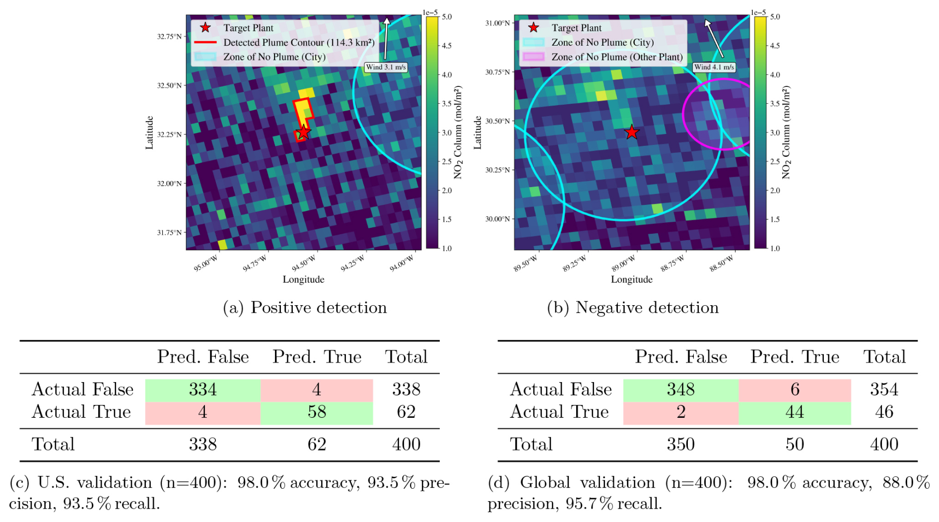
Figure 5 Validation of the Automated Plume Detection Algorithm. (a) A positive-detection example (TROPOMI overpass 26 July 2022 19:25:10 UTC): the algorithm identifies a plume attributable to the target power plant. (b) A negative-detection example (TROPOMI overpass 26 July 2022 19:24:27 UTC): the target plant's location lies inside an interference-zone mask (no-plume zone) defined in Step 1, so the algorithm returns no plume. Outside the mask, a detection would additionally require the dual-threshold conditions of Step 5 (statistical significance and absolute minimum) and the minimum plume-area condition of Step 2 to be met. (c, d) Confusion matrices for the US and global validation samples. “True” denotes the presence of a plume attributable to the target plant and “False” denotes its absence; “Predicted” is the algorithm's binary output and “Actual” is the manual human label assigned to the same observation. Green cells are correct classifications (TN and TP) and red cells are misclassifications (FP and FN). (c) The US validation uses 400 observations stratified across five emission quantiles (∼ 80 per bin). (d) The global validation uses 400 observations jointly stratified across six continents and five emission quantiles (∼ 13 per cell, 80 per emission bin). Dataset: two manually labeled validation sets (n=400 US, n=400 global) sampled from the full quality-filtered dataset (n=666 222 US/n=875 686 global TROPOMI observations).

In the first test, we evaluated US performance using an emission-stratified validation set of 400 US observations, with 80 observations per emission-level quantile defined above. Manual verification of this set provides a benchmark for US performance across the emission range. Figure 5c shows the resulting confusion matrix, with an overall accuracy of 98.0 % (precision 93.5 %, recall 93.5 %).

In the second test, we assessed robustness by constructing a continent-and-emission-stratified global validation set of 400 observations. Observations were drawn from the global dataset by jointly stratifying across the same five emission-level quantiles and across six continents (roughly 13 observations per (continent, quantile) cell, yielding 80 observations per emission bin); we drop Antarctica because it contains no power plants in our inventory, and observations whose ISO3 country code does not map to one of the six continents are excluded prior to sampling. On this stratified global set, the algorithm achieved an accuracy of 98.0 % (precision 88.0 %, recall 95.7 %), as shown in Fig. 5d.

3.3 Training Sample Filtering

Beyond the per-scene masking applied within the labeling algorithm (Sect. 3.2), we apply a plant-level filter to construct the dataset for the second-stage detectability analysis: we retain only plants that lie outside interference zones across every analyzed year, giving a cleaner dataset.

We first find that for the US Top 500 NO_x emitters (2019–2024), 312/500 plants (62.4 %) were flagged as in interference zones in 2019, declining to 283 by 2024 as the number of active plants shrank from 500 to 461. Metropolitan proximity remains the primary driver of interference. Across six years, only 171 plants were never within interference zones, accounting for 45.0 % of emissions from the original 500.

Interference is even more pervasive in the global dataset of 6000 major power plants. In total, 4935 plants (82.3 %) lie within at least one interference zone; proximity to large urban centers dominates (4491 plants), while co-located power plants also contribute substantially (2719 plants). Notably, 2275 plants are simultaneously affected by both cities and other plants, underscoring the difficulty of identifying interference-free monitoring conditions at scale. In 2018, only 1065 plants remained outside interference zones, retaining just 21.1 % of the original emissions.

These contrasting retention rates, 45.0 % for US plants versus 21.1 % for global plants, reflect the higher spatial clustering of emission sources and urban areas in the global dataset.

Table 2 Subset-level observation filtering. “Retained” is the modeling subset, i.e., observations with no missing input features, target plant outside interference zones, and (for US rows) a paired CAMPD record. Dataset: full quality-filtered dataset (n=666 222 US and n=875 686 global TROPOMI observations), with each “Top X” row restricted to the Top X NO_x emitters.

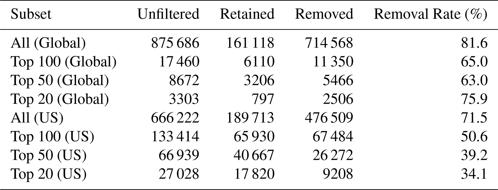
At an observation level, requiring (i) no missing values in any input feature, (ii) a valid paired NO_x record (CAMPD for the US, CoCO₂ for global), and (iii) a target plant outside interference zones, the final modeling subset retains 189 713 of 666 222 US observations (71.5 % excluded across 2019–2024) and 161 118 of 875 686 global observations (81.6 % excluded). To support the per-emission-magnitude analyses described later (Sect. 3.4), we also consider three subsets defined by the highest-emitting plants within each region: the Top 100, Top 50, and Top 20 by total NO_x emissions. Table 2 reports removal rates for these smaller US subsets, which are similarly large.

While this filtering is stringent, it is necessary to ensure interpretability and causal attribution. Our goal is to analyze how meteorology, emission rate, and environmental factors affect plume visibility, not to model column enhancements that may arise from overlapping sources. Without isolating interference-free scenes, plume detections could be driven by emissions from neighboring plants or urban NO₂ backgrounds, obscuring the true relationships between plant-level conditions and observed plume visibility. Thus, the reduced sample size reflects a trade-off: a smaller but cleaner dataset that supports robust inference about the mechanisms underlying visible plumes in satellite imagery.

3.4 Plume Detectability Prediction

Using the dataset constructed in Sect. 3.3, we train a machine learning model to predict plume detectability from the input features. We frame plume detectability as a binary classification task. For each TROPOMI observation, which our algorithm labels as either “plume detected” or “no plume,” we extract a comprehensive set of meteorological, sensor, environmental, and power-plant features to use as classifier inputs.

We use a Multi-Layer Perceptron (MLP) for this binary classification task. The MLP is a fully-connected feedforward network with four hidden layers (256, 128, 64, and 32 neurons) using ReLU activation functions. To mitigate overfitting, we apply dropout (p=0.3) after the first three hidden layers. The network takes 25 input features (24 numeric features plus the integer-encoded primary fuel type) and produces a binary classification output, giving 49 921 learnable parameters. This architecture is used for all US and global analyses.

To understand how performance varies with emission magnitude, we trained separate models on four datasets: “All” (the full modeling subset of Sect. 3.3) and the three highest-emitter subsets (“Top 100”, “Top 50”, and “Top 20”) defined in Sect. 3.3. For each dataset, we partitioned observations into training (60 %), validation (20 %), and test (20 %) sets.

We addressed class imbalance in the training set using random oversampling and then standardized all input features to have zero mean and unit variance, based on the resampled training data statistics. We trained each model to maximize the Area Under the Curve (AUC) on the validation set. To account for training stochasticity, we repeated each experiment five times and reported the mean and standard deviation of the results. Full training details are in Sect. S3 in the Supplement.

We evaluate two complementary splits: an item split, in which observations are randomly assigned to train, validation, and test sets (in-distribution generalization), and a power plant split, in which entire plants are held out for testing (out-of-distribution generalization to unseen facilities). For each model we report six standard classification metrics (Accuracy, Precision, Recall, F1, AUC, and Cohen's κ); item-split results are presented in Sect. 4.3 and power-plant-split results in Sect. S5 in the Supplement.

3.5 Permutation Score and SHAP Score Estimation

3.5.1 Model-wide Feature Importance via Permutation

To assess the model's overall reliance on each input feature, we use permutation importance, a technique well-suited for complex models like MLPs. For a given feature x_i and the held-out test set 𝒟_test, we first calculate the model's baseline performance, ℳ_orig, using a chosen metric like AUC. We then randomly shuffle the values of only feature x_i across all examples in 𝒟_test to break its relationship with the target variable, and we re-evaluate the model to get a permuted performance score, ℳ_perm(i). The permutation importance of feature x_i is the resulting drop in performance:

$$\begin{array}{}\text{(1)}& {\mathrm{\Delta }}_i={\mathcal{M}}_{\text{orig}}-{\mathcal{M}}_{\text{perm}\left(i\right)}.\end{array}$$

A larger value of Δ_i signifies that the model depends more heavily on that feature for its predictions.

3.5.2 Plant-Level Feature Importance via SHAP

While permutation importance gives a global view, we use SHAP (SHapley Additive exPlanations) to explain predictions for individual power plants in the held-out test set 𝒟_test. SHAP assigns an importance value, ϕ_i, to each feature based on its marginal contribution to a specific prediction. For a plant with feature vector x∈ℝ^d (d=25 in our case), these SHAP values explain how the model's prediction, f(x), deviates from the baseline prediction, E[f(X)], where X is the random feature vector over the dataset and x is a specific plant's realization:

$$\begin{array}{}\text{(2)}& f\left(\mathit{x}\right)-E\left[f\right(\mathit{X}\left)\right]=\sum _{i=\mathrm{1}}^d{\mathit{\varphi }}_i.\end{array}$$

The exact computation of these Shapley values requires re-evaluating the model on all possible subsets of features, which is computationally prohibitive for any non-trivial number of features. We therefore estimate them using the SHAP DeepExplainer algorithm. This method, based on a deep learning attribution technique called DeepLIFT, efficiently approximates SHAP values. It works by propagating the difference between the model's final output and a baseline reference output backwards through the network layers. This process assigns contribution scores to each neuron and, ultimately, to each input feature, providing a tractable approximation for neural networks like our MLP.

Each value ϕ_i quantifies how much feature i pushes the prediction away from this baseline. A positive ϕ_i increases the predicted detectability, while a negative value decreases it. Ranking the absolute SHAP values, $\left|{\mathit{\varphi }}_i\right|$, reveals which features most strongly drive the outcome for a single plant.

To visualize these local explanations on a global scale, we aggregate the plant-level SHAP results onto a grid, as shown in Fig. S2 in the Supplement. First, we assign each power plant to a grid cell. Within each cell, we identify the most influential feature by finding which feature most frequently has the highest absolute SHAP value ($\left|{\mathit{\varphi }}_i\right|$) across all plants in that cell. Next, we determine that feature's dominant directional impact (positive or negative) within the cell. The final map visualizes these results, with each cell colored by its dominant feature and marked with an arrow indicating its typical influence on plume detectability.

4 Results

4.1 Scope of the analysis

After interference filtering (Sect. 3.3), the analyzed set consists of 171 US plants outside interference zones (retaining 45.0 % of the original NO_x emissions from the Top 500 selection) and 1065 global plants outside interference zones (retaining 21.1 % of the original NO_x emissions from the Top 6000 selection); 189 713 of 666 222 US observations and 161 118 of 875 686 global observations remain. All detectability results in the following subsections refer to this filtered set.

4.2 NO₂ plume detectability has regional disparities

With power plants near interfering emitters removed, we proceeded with a clean set of observations in which emissions can be attributed to the target power plant. We apply the pipeline to 500 US plants (January 2019–December 2024) and 6000 global plants (May–December 2018), excluding power plants within interference zones. Detection frequency varies dramatically across sites.

In the United States (171 after filtering with full 6-year availability), detections range from 11 to 258 per plant on average each year, with a median of 48. This range is highly uneven: plants at P₉₀ (154 detections yr⁻¹) record about 8.6× more detections per year than those at P₁₀ (18 detections yr⁻¹). When adjusted for the number of satellite overpasses, the per-plant detectability spans from 6.0 % to 85.2 % (median 20.4 %; P₁₀ = 10.0 %, P₉₀ = 63.7 %).

Globally (1065 plants after filtering), detections over the eight-month period in 2018 range from 0 to 251, with a median of 38. Plants at P₉₀ (141 detections) record about 11.8× more detections than those at P₁₀ (12 detections). When adjusted for the number of satellite overpasses, the per-plant detectability spans from 0 % to 100 % (median 27.8 %; P₁₀ = 10.5 %, P₉₀ = 81.8 %).

Detection frequency is strongly correlated with empirical detectability across plants (Pearson r=0.96 for the US and r=0.89 for the global dataset), as expected since detection frequency is the product of detectability and the number of valid overpasses.

These per-plant detectability estimates are consistent between the two independently configured pipelines: on the 160 plants present in both runs (matched within < 10 m), the US and global per-plant detectabilities agree closely (Pearson r=0.96; Fig. 6), despite differences in emission temporal resolution (hourly CAMPD vs. annual CoCO₂) and observation period (2019–2024 vs. 2018). The small residual offset (mean +0.036; US mean 0.163 vs. global 0.199) likely reflects the temporal gap, since US NO_x emissions have continued to decline over 2019–2024.

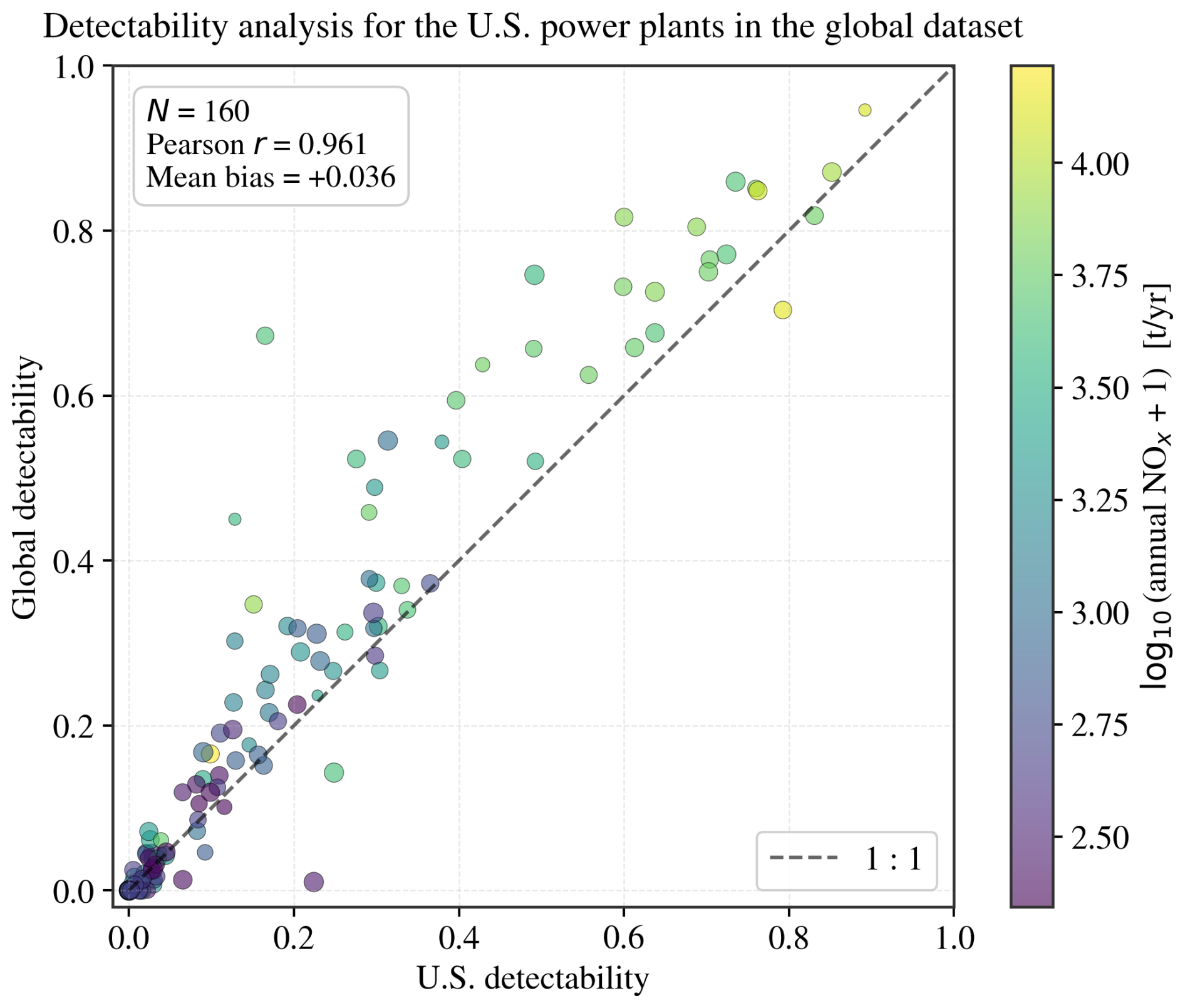
Figure 6 Per-plant detectability comparison between the US pipeline (2019–2024) and the global pipeline (2018) for the 160 plants present in both runs (matched within < 10 m). Each point is a plant, colored by log ₁₀ of the CoCO₂ annual NO_x emissions (in t yr⁻¹, with a +1 offset for plants near zero). The dashed diagonal marks 1:1 agreement. Pearson r=0.961; mean bias = +0.036. Dataset: full quality-filtered dataset (n=666 222 US and n=875 686 global TROPOMI observations).

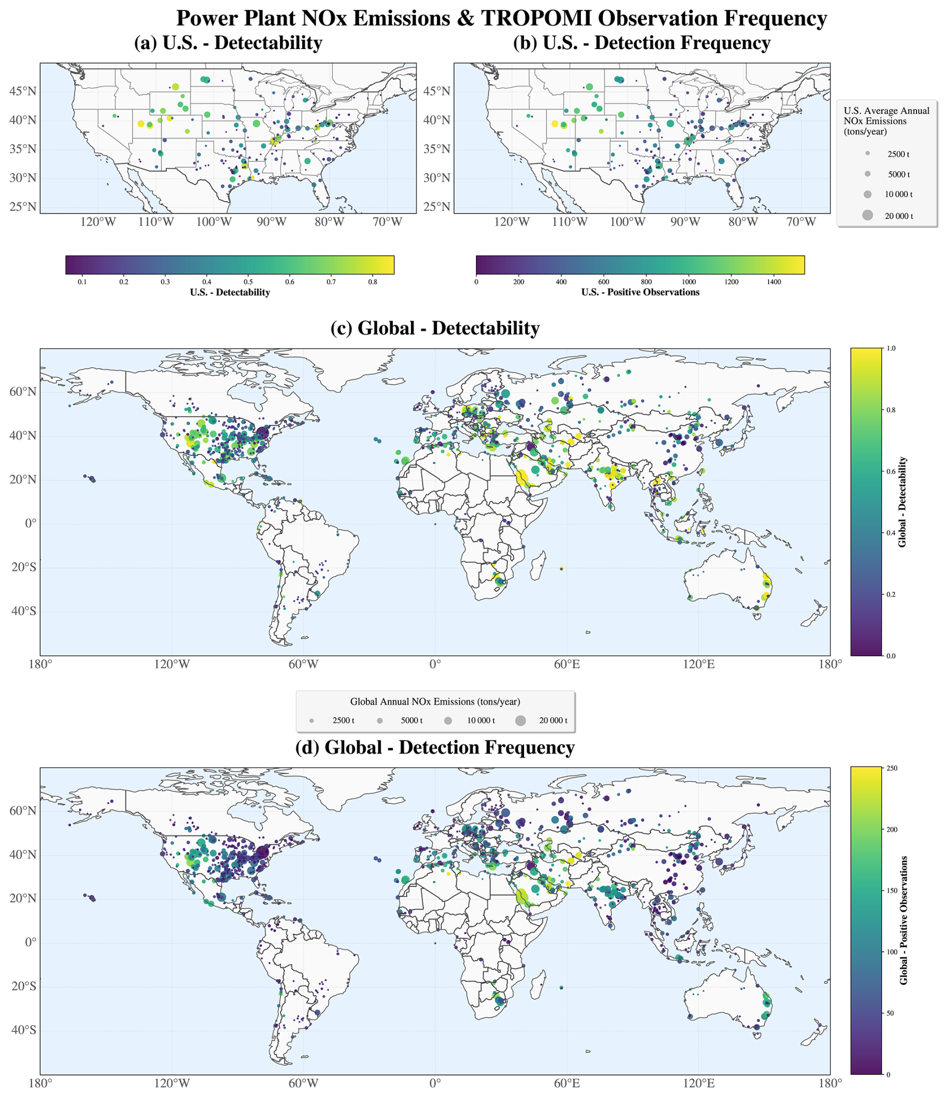
Figure 7 Maps of NO_x emissions and TROPOMI observations: marker size ∝  annual NO_x (metric t yr⁻¹) at each plant, with US panels colored by (a) plume detectability and (b) detection frequency, and global panels colored by (c) plume detectability and (d) detection frequency. Dataset: per-plant aggregate over the full quality-filtered dataset, restricted to interference-free plants with no missing-feature filter applied (171 US plants, n=234 038 observations; 1065 global plants, n=161 143 observations).

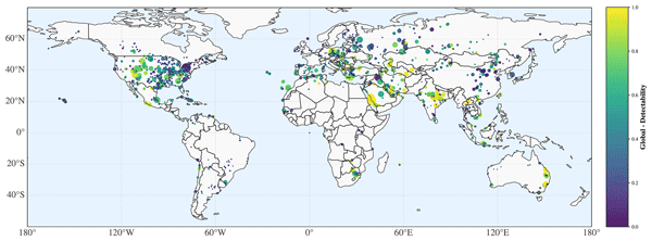
These disparities have a clear geographical distribution: detectability is higher in arid and semi-arid regions (e.g., the US interior West and Great Plains, Iberia, North Africa, Greece/Turkey, central Brazil/Argentina, eastern Australia) and lower in humid regions. Notably, the detectability of plants with the same level of emissions varies across different geographical regions, highlighting that emissions alone are insufficient to predict detectability. Regional meteorology and surface properties also strongly affect plume detectability, as visible in Fig. 7a and c; we revisit these geographic patterns in Sect. 4.4 in light of the feature-importance results.

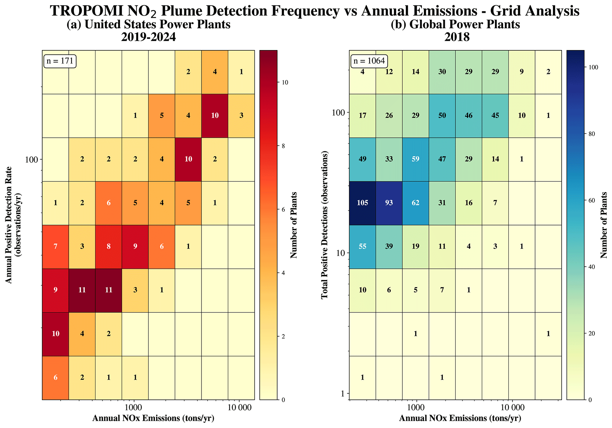
Figure 8 TROPOMI NO₂ plume detection frequency versus annual NO_x emissions. (a) US plants (n=171, retaining 45.0 % of emissions from the original 500 plants). (b) Global plants (n=1065, retaining 21.1 % of emissions from the original 6000 plants); 1064 plants are plotted, as one plant yielded no positive detections. Numbers denote plant counts per grid cell (8×8 log-uniform bins). Dataset: per-plant aggregate over the full quality-filtered dataset, restricted to interference-free plants with no missing-feature filter applied (171 US plants, n=234 038 observations; 1065 global plants, n=161 143 observations).

Despite this aggressive filtering, satellite detection frequencies remain remarkably high, as shown in Fig. 7. All 171 US plants exhibit detection frequencies exceeding 10 observations per year, with 87.7 % detected more than 20 times annually and nearly half (46.2 %) detected more than 50 times per year. The global dataset shows similarly strong performance, with 93.3 % of plants detected more than 10 times and three-quarters (75.1 %) detected more than 20 times during the eight-month observation period. Figure 8 further shows that 24.6 % of US plants exceed 100 positive detections per year and 19.8 % of global plants exceed 100 positive detections over the eight-month period, demonstrating TROPOMI's capability for frequent monitoring even after conservative spatial filtering. Detection frequency generally increases with emission magnitude, though substantial variability exists within emission bins, likely reflecting differences in meteorological and environmental conditions across facilities.

Table 3 Multi-Layer Perceptron performance (item split) for US and global datasets. Dataset: modeling subset (Sect. 3.3; 171 US plants, n=189 713 observations; 1065 global plants, n=161 118 observations); each “Top X” row uses the corresponding subset of Table 2.

4.3 Plume detectability is predictable with high accuracy across US and global datasets

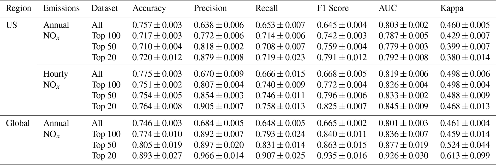
We report results from the two split designs introduced in Sect. 3.4. Table 3 reports the item-split results for both US and global datasets; the power-plant-split results are reported in Table S2 in the Supplement (Sect. S5). The tables organize performance by region, emission data resolution (annual vs. hourly NO_x), and dataset scope (All vs. Top X emitters). Of the six classification metrics reported, we focus discussion on Precision, Recall, and the F1 score, which together quantify the reliability of positive predictions, the ability to capture all true events, and the balance between these competing objectives in operational monitoring.

Our model predicts plume detectability from meteorological and emissions features with high accuracy. As reported in Table 3, across US and global datasets, the multi-layer perceptron reaches 0.75–0.78 accuracy, 0.65–0.67 F1 score and achieves AUCs above 0.80; the underlying receiver operating characteristic (ROC) curves for the “All” subset are shown in Fig. S1 in the Supplement (Sect. S4.1). These metrics show that sensor, power plant, meteorological, and environmental variables can predict plume detectability, though imperfectly. The residual errors suggest that key drivers are either unmeasured or captured too coarsely, limiting the separability between detectable and undetectable plumes.

Model performance improves when focusing on high-magnitude emitters, as seen by comparing the “All”, “Top 100”, “Top 50”, and “Top 20” rows of Table 3, where each row corresponds to a separate model trained and evaluated on the indicated subset (Sect. 3.4). As the subset is restricted to higher emitters, Precision, Recall, and the F1 score all rise, with Precision showing the largest improvement. This trend suggests that on these subsets the model makes fewer false positive errors, since stronger emitters tend to produce less ambiguous plume signals.

We note that the slight decrease in accuracy in the US when focusing on high emitters is caused by a significant shift in class balance. The full dataset contains a large number of “undetectable” cases (true negatives), and the model correctly identifies them, boosting the overall accuracy score. When the dataset is filtered to only the top emitters, these easier-to-classify negative cases are removed.

Though the global dataset uses coarser temporal emission data, the model trained on it matches or exceeds the model trained on the US dataset across all subsets, with the gap widening for the highest emitters (e.g., on Top 20, Global F1 = 0.935 vs. US hourly F1 = 0.825). This may initially appear surprising; we speculate that the broader variability in environmental variables and emissions in the global dataset sharpens the boundary between detectable and undetectable cases, helping the global-trained model generalize better.

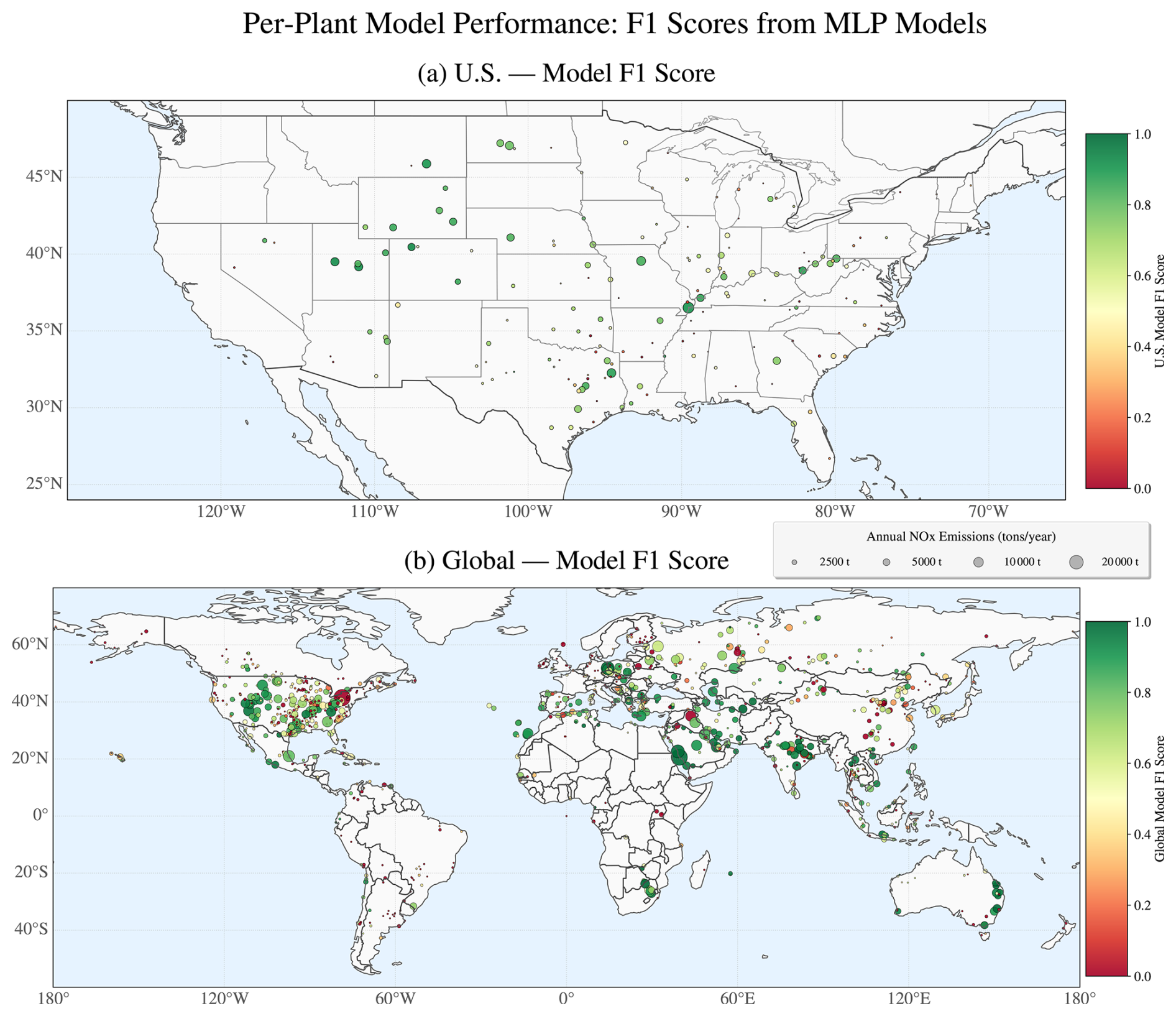
Figure 9 Geographic distribution of multi-layer perceptron (MLP) model performance in detecting NO₂ plumes from individual power plants, evaluated using the F1 score. Panel (a) shows results for the US model, while panel (b) presents the global model. Each point represents a power plant, with color indicating predictive performance on a scale from 0.0 (poor) to 1.0 (perfect), and marker size proportional to annual NO_x emissions. We can see a general trend that larger emitters tend to have higher F1 scores. The US model demonstrates strong performance over Midwest areas. The global model demonstrates strong performance across North America, Europe, and the Arabian Peninsula. For each plant, the F1 score is computed over all of its observations across the train, validation, and test splits. Dataset: modeling subset (Sect. 3.3; 171 US plants, n=189 713 observations; 1065 global plants, n=161 118 observations).

To understand how model performance varies across the world, we performed a spatial analysis of F1 scores for individual power plants. Figure 9 shows the geographic distribution and reveals distinct regional patterns in model accuracy. For the US-trained model (Fig. 9a), performance is strongest in the Midwest and parts of the Western US, where the model achieves F1 scores consistently above 0.8 for major emitters. The globally trained model (Fig. 9b) demonstrates robust performance across industrialized regions including North America, Europe, and the Arabian Peninsula, with F1 scores often reaching 0.8–1.0 for large point sources. Performance degrades in parts of Asia, South America, and Africa, where F1 scores show greater variability and often drop below 0.5, likely because training data are sparser and emissions are lower in these regions. The sparser training data in these regions are themselves partly a consequence of factors that make satellite retrievals more difficult there, including high aerosol load, water vapor, and persistent cloud cover, which reduce the number of high-quality TROPOMI observations available for analysis. Across all regions, a clear positive relationship exists between emission magnitude (point size) and model performance: larger NO_x emitters are detected with higher accuracy, likely because stronger plume signals exceed detection thresholds more reliably; this relationship is verified in Fig. S3 in the Supplement.

One notable outlier appears in the northeastern US. The global model shows poor performance for what appears to be the largest emitter in the US after interference zone filtering in the CoCO₂ dataset, yet this facility is absent from the US analysis. This facility, Domtar Paper Company, LLC, reports 2018 NO_x emissions of only 35.57 t in the EPA dataset but 29 652 t in CoCO₂, an ∼ 830-fold discrepancy. If the EPA data are correct, the facility's small actual size explains the poor detectability. In other words, the CoCO₂ dataset is likely incorrect about Domtar Paper Company's emissions.

4.4 Which features are most predictive of plume detectability?

To identify the key predictors of NO₂ plume detectability, we performed a permutation importance analysis on our best-performing models from Table 3. Figure 10 (left) shows the ranked feature importance, sorted by the combined US and global importance. The top 5 features are NO_x emission rate, surface altitude, surface albedo (NO₂ window), sensor zenith angle, and primary fuel type, with wind speed close behind at rank 6. Our SHAP score analysis yielded similar results, which are shown in Sect. S4.2 in the Supplement. A complete list of permutation-importance values appears in Table S3 in the Supplement (Sect. S6). Cloud fraction appears low in this ranking, but still shapes detectability within the post-quality-assurance range (quality flag >0.75); we show this in Sect. S6.2 in the Supplement.

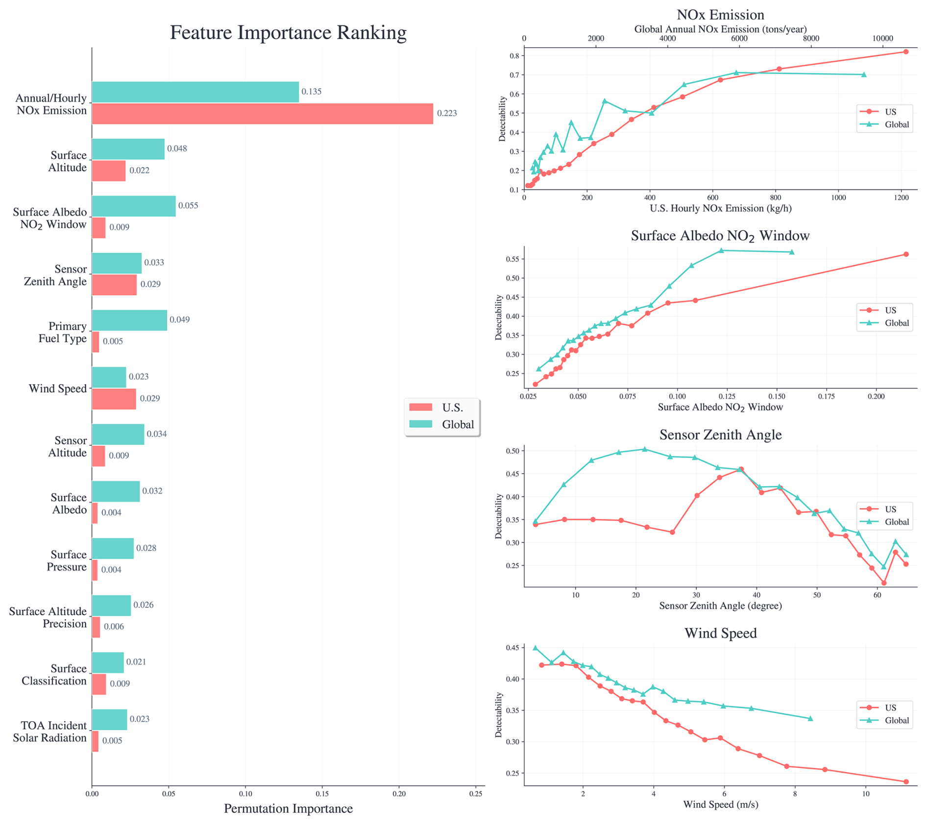
Figure 10 Feature importance and detectability analysis for TROPOMI-based NO₂ models at US (red) and global (teal) scales. Left: ranked permutation importance for the top 12 features, sorted by the sum of US and global importance and computed on the held-out test split of the dataset. Right: detectability as a function of NO_x emission rate, surface albedo (NO₂ window), sensor zenith angle, and wind speed, computed on the dataset. Binning uses a quantile-based strategy (1st–99th percentile) to ensure balanced feature distribution and avoid extreme values. Dataset: modeling subset (Sect. 3.3; 171 US plants, n=189 713 observations; 1065 global plants, n=161 118 observations); the held-out test split contains n=37 943 US and n=32 224 global observations.

To examine how these features shape detectability, we employ a quantile-based binning strategy, using data between the 1st and 99th percentiles. This approach ensures a balanced distribution of observations across bins while mitigating the influence of extreme outliers. We grouped the data into 20 quantile bins for each feature (≈ 7900 observations/bin globally; ≈ 9300 in the US) and computed the detectability within each bin. While we acknowledge that these variables can be correlated, we find the trends persist when we parse the data to isolate each feature's effect (e.g., by holding other variables roughly constant). The resulting curves, plotted against the corresponding feature values, are shown in the right panel of Fig. 10.

Detectability increases with both emission rate and surface albedo. As expected, higher emissions increase NO₂ concentration and therefore the detectable signal, while brighter surfaces increase scene radiance, improving signal-to-noise ratio (SNR). This albedo dependence is consistent with the geographic patterns reported in Sect. 4.2: arid and semi-arid regions have higher detectability partly because of their elevated surface albedo, while humid regions are penalized by both lower albedo and more frequent cloud cover. Our analysis finds that for US power plants, an average hourly emission rate of ≈ 400 kg h⁻¹ corresponds to a ∼ 50 % detectability. The result for global power plants is similar, although the global P(detect) versus NO_x emission curve is slightly above the US curve. To compare US and global performances in Fig. 10, we align their emission axes to share the same numerical scale, despite the different units (kg h⁻¹ for the US, t yr⁻¹ for global). We align the x-axis for US emissions (kg h⁻¹) and global emissions (t yr⁻¹) by converting the US hourly rates to annual values using 24 × $\mathrm{365}/\mathrm{1000}$, allowing direct comparison with the global annual rates. The US curve consistently falling below the global curve suggests that the premise of continuous operation is often invalid, as many US plants run intermittently, leading to lower detectability.

By contrast, the sensor zenith angle (VZA) shows a hump-shaped dependence, with mean peak plume detectability near 20° VZA globally and 35° in the US. Two effects can possibly explain the rising flank. First, retrievals measure NO₂ slant column density along the line of sight and convert it to vertical column density by dividing by the AMF; at higher VZA the longer slant path yields a larger AMF (Palmer et al., 2001), so the same slant-column noise translates into a smaller vertical-column noise. Lower background noise raises detection probability at fixed plume signal. Second, for the US analysis period our 25 km² flagged-area threshold introduces a pixel-quantization step: TROPOMI pixel area grows from ∼20 km² at nadir to ∼25 km² near VZA =26° for the 3.5 km × 5.5 km pixels available from August 2019 onwards (Fig. S7 in the Supplement), so detection requires ≥2 contiguous flagged pixels below 26° but only one above, producing a step increase in detectability. At larger VZA, detectability falls as radiance drops, multiple scattering grows, the larger pixel size dilutes the plume signal more strongly, and retrieval uncertainty increases under oblique geometry (Van Geffen et al., 2020).

Finally, wind speed is negatively correlated with detectability. Stronger winds advect and dilute plumes, lowering column contrast and thus detectability. We note that this is different from the ideal wind speeds for quantifying emissions, which prior literature shows to occur at moderate wind speeds (2–4 m s⁻¹) (Bruno et al., 2024). Very low wind speeds make it difficult to quantify the rate of emission due to the high relative uncertainty in the wind measurement itself, while the same plume dilution that hinders detection at very high wind speeds also introduces large errors into the quantification algorithm (Bruno et al., 2024). These two relationships are not in conflict because detection and quantification address different tasks: quantification requires a coherent plume structure that the retrieval can fit, which breaks down at very low wind (no advection); detection only asks whether any NO₂ enhancement is present at the source, which is favored by low wind because NO₂ accumulates near the source.

Primary Fuel Type is a significantly less important feature in the US model (feature importance: 0.005) compared to the global model (feature importance: 0.049). This difference likely stems from the relative homogeneity of the US power sector in both its fuel sources and emission controls. First, the Top 500 US emitters are dominated by gas- and coal-fired plants: of the 461 plants still reporting in 2024, ≈ 56 % burn gas (pipeline natural gas, natural gas, other gas, or process gas) and ≈ 39 % burn coal or coal refuse, leaving ≈ 4 % on other fuels and ≈ 1 % with no reported fuel type. This low fuel variability is in stark contrast to the global dataset. While also led by coal (≈ 50 %) and natural gas (≈ 30 %), the global mix is far more diverse, including substantial shares of facilities running on oil (≈ 12 %), biomass (≈ 6 %), and waste (≈ 2 %). Second, this effect is compounded by emission controls. In the US, power plants are subject to relatively uniform and stringent environmental regulations, such as the Clean Air Act, often requiring technologies like Selective Catalytic Reduction to control NO_x emissions. Globally, however, the presence and effectiveness of these technologies vary drastically by country. In that context, fuel type can serve as a stronger proxy for a facility's overall emission profile.

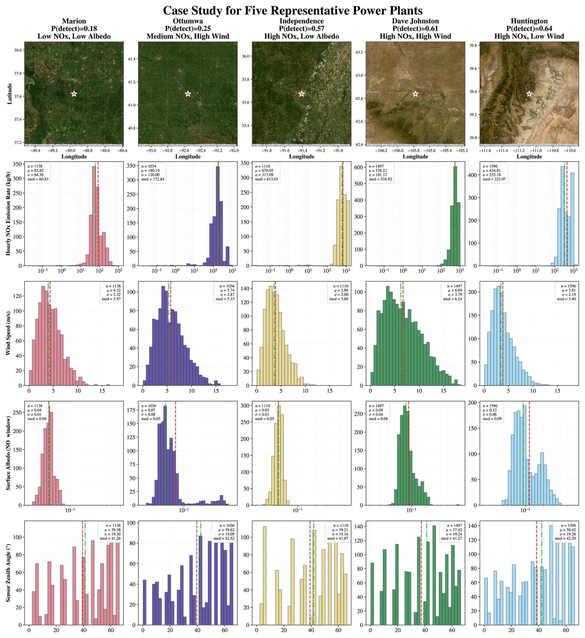
Figure 11 Variable distributions for five representative power plants demonstrating detectability drivers. Plants were selected to showcase diverse NO_x emissions, meteorological conditions, and viewing geometries. Top: Satellite imagery with detectability values and dominant characteristics. Rows 2–5: Histograms of hourly NO_x emission rates (kg h⁻¹), wind speed (m s⁻¹), surface albedo (NO₂ window), and sensor zenith angles, with mean (red dashed) and median (green dash-dot) lines. Consistent scales enable cross-plant comparison. Basemap: ArcGIS World Imagery (Powered by Esri) (Esri, 2026) via contextily (Arribas-Bel and contextily contributors, 2024). Dataset: five US plants drawn from the 171 plants of the US modeling subset (Sect. 3.3; n=189 713 observations); each histogram uses the selected plant's observations from this subset.

While the feature importance analysis identifies the key predictors and their marginal effects, real-world plume detectability emerges from the combined influence of multiple interacting factors. To illustrate how emission rates, albedo, and wind speed operate in concert at individual facilities, we examine in Fig. 11 five representative power plants that span the range of conditions observed in our dataset. Marion, with low NO_x emissions (∼ 83 kg h⁻¹) and low albedo (0.04), has the lowest detectability (P(detect)=0.18). Ottumwa shows higher NO_x (∼ 180 kg h⁻¹) but experiences high wind speeds (5.74 m s⁻¹) and a low but highly variable albedo (mean ≈ 0.07, with a long tail from winter snow cover), yielding P(detect)=0.25.

Comparing Marion and Independence directly demonstrates the dominant effect of emission rate: Independence's high NO_x (∼ 670 kg h⁻¹) achieves P(detect)=0.57 despite similarly low albedo (0.05). Among the three high-emitting plants (Independence, Dave Johnston, Huntington), surface characteristics and wind become the limiting factors. Independence's low albedo constrains detectability to 0.57, while Dave Johnston (high wind, 6.69 m s⁻¹; albedo 0.09) reaches 0.61, and Huntington (low wind, 3.81 m s⁻¹; high albedo, 0.12) achieves the highest detectability at 0.64. These examples demonstrate that high surface albedo and low wind enhance NO₂ retrieval sensitivity even when emission rates are comparable.

5 Discussion

This study provides the first global, data-driven quantification of when and where power-plant NO₂ plumes are visible from space. Previous satellite analyses of power plants have typically examined a handful of large facilities under selected conditions to estimate emissions (Goldberg et al., 2019; Beirle et al., 2019; Liu et al., 2020; Cusworth et al., 2021). In contrast, we analyze more than 6000 facilities worldwide using a consistent, automated plume-detection and machine-learning framework that links satellite detectability to meteorological, environmental, sensor, and power-plant features. Our goal in establishing empirical relationships governing plume visibility is to elucidate the current limits of satellite NO₂ sensing and inform future satellite-based NO_x emission quantification.

5.1 Empirical characterization of plume detectability

Our results empirically confirm several theoretical expectations from satellite trace-gas retrieval physics while quantifying their combined effects on plume visibility at global scale. Viewing geometry exerts a strong nonlinear influence: moderate off-nadir angles enhance detectability by increasing the optical path length through the lower troposphere, consistent with established AMF and averaging-kernel theory (Palmer et al., 2001; Eskes and Boersma, 2003). At larger angles, detectability declines as scene radiance decreases and multiple scattering increases (Van Geffen et al., 2020). Surface reflectance also plays a major role, with higher albedo increasing scene radiance and retrieval SNR, improving the contrast between a plume and its background, consistent with TROPOMI characterization studies (Van Geffen et al., 2020).

Our analysis extends these theoretical principles by quantifying their global impact empirically. Across thousands of facilities, detectability peaks at intermediate sensor zenith angles (near 20° globally and 35° in the US) and increases monotonically with both emission rate and surface brightness. For the US subset, an average hourly NO_x emission rate of roughly 400 kg h⁻¹ corresponds to a ∼ 50 % detectability. These results provide the first global observational confirmation of how viewing geometry, surface brightness, meteorology, and emission strength jointly control satellite plume visibility.

5.2 Implications for emission retrieval

The same meteorological, environmental, sensor, and power-plant variables that determine whether a plume is detectable also shape how it appears in satellite imagery. Wind speed controls plume width and dispersion, solar and sensor geometry set the radiative contrast and effective path length, and surface albedo defines the background brightness against which NO₂ enhancements are retrieved. If these factors affect visibility, then they also influence the quantitative mapping between observed plume morphology/enhancement and underlying emissions. Consequently, emission-retrieval frameworks, whether physics-based inversions or machine-learning models, are likely to benefit by explicitly incorporating these variables. In inverse modeling, detectability probabilities or their underlying covariates could serve as weights or priors, emphasizing scenes with favorable observing conditions and reducing biases introduced by low-sensitivity observations. In machine-learning-based retrievals, including features such as wind speed, solar/sensor angles, and surface albedo alongside the imagery would allow models to learn how identical plume appearances can correspond to different true emissions under different conditions. This contextual information should improve generalization across power plants and climates, reduce bias in data-poor regions, and produce more physically consistent emission estimates.

We emphasize that detectability as defined here is necessary but not sufficient for emission quantification: it characterizes the upstream observational limit (whether any NO₂ enhancement attributable to the plant is present in the scene), whereas quantification additionally requires that the plume's structure be sufficiently coherent to recover an emission rate. The conditions favorable for detection and for quantification therefore overlap but are not identical; for example, low wind favors detection (because NO₂ accumulates near the source) but is unfavorable for quantification methods that require a clearly advected plume.

5.3 Robustness to inventory uncertainty

A natural concern is that the reported emission rates used as a predictor are themselves uncertain. Reported inventories disagree both with satellite-derived estimates (e.g., Beirle et al., 2019; Goldberg et al., 2019) and among themselves (e.g., EDGAR (Crippa et al., 2022) vs. E-PRTR (European Environment Agency, 2020)). Within the global subset we use CoCO₂ annual emissions (Guevara et al., 2024), while the US subset uses hourly emissions (U.S. Environmental Protection Agency, 2023).

Two factors degrade the signal the model can extract from the reported emissions: noise in the reported inventories, and the use of annual emissions for the global subset (the only data available at global scale), which is a less faithful proxy of the emissions at each observation.

To make the first factor concrete: because NO_x emission rate is the model's most important predictor (Sect. 4.4), a plant that over-reports its emissions is presented to the model with a high emission value, leading it to predict high detectability; yet TROPOMI detects the plume less often than expected because the true emissions are lower, so the prediction overshoots. A plant that under-reports produces the opposite error.

These errors propagate in two ways. First, the reported F1 and AUC values should be read as lower bounds on the model performance achievable under cleaner inputs. Second, the same noise feeds into our feature-importance estimate, so that NO_x emission rate appears less important than it truly is. Its top SHAP ranking is therefore a conservative lower bound, and access to cleaner inventories, including global hourly data, would only strengthen this ranking.

5.4 Implications for upcoming high-resolution missions

Several new and forthcoming satellite missions are moving point-source plume sensing toward spatial resolutions finer than TROPOMI's 3.5–7 km pixels. GOSAT-GW/TANSO-3 targets 1–3 km footprints in Focus Mode (Japan Aerospace Exploration Agency, 2024), CO2M will provide collocated CO₂, CH₄, and NO₂ through CO2I/NO2I at ∼ 4 km² (Sierk et al., 2021), and TANGO-Nitro targets facility-scale NO₂ imaging at ∼ 300 m (Landgraf et al., 2020). How do the TROPOMI-scale relationships quantified here translate to sensors with smaller footprints? We discuss implications for plume detectability and feature importance in turn.

Spatial resolution affects detectability through competing mechanisms. First, a smaller instantaneous field of view reduces mixing between the plume and background, so a point-source enhancement may be less diluted within a pixel. Second, finer pixels can reduce interference from neighboring power plants and cities. This is particularly relevant for our study because interference filtering excludes a large fraction of plants from the second-stage detectability analysis. Higher-resolution sensors could therefore allow more power plants, and a larger fraction of global emissions, to be characterized. Third, for a fixed instrument design, smaller pixels collect fewer photons, which can increase retrieval noise and background variability. Thus finer spatial resolution should improve plume detection when TROPOMI is limited by plume dilution or source interference, but this gain depends on maintaining sufficient SNR and retrieval quality.

How feature importance changes at finer spatial resolution is harder to predict. The important features identified in Fig. 10 should be interpreted as properties of the TROPOMI retrieval, TROPOMI pixel size, the detection algorithm, and the sampled observation conditions, rather than as feature rankings that transfer unchanged across sensors. Surface albedo and surface altitude are especially important examples. In our TROPOMI-based model, these variables may influence detectability both by affecting retrieval and by acting as proxies for systematic bias associated with unresolved surface heterogeneity. Recent work on CO2M-like retrievals shows that correlated subpixel variations in surface reflectance and altitude can produce retrieval biases, and that improved subpixel surface characterization can reduce those biases (Weimer et al., 2026). At finer resolution, some of the apparent importance of albedo or altitude could therefore decrease if it currently reflects unresolved subpixel bias. Repeating our analysis for higher-resolution sensors would show which predictors remain dominant across instruments and which are specific to TROPOMI-scale retrieval and resolution. We leave this comparison to future work.

6 Conclusions

In this work, we systematically mapped power plant NO₂ plume detectability at US and global scales using TROPOMI observations (nadir pixel size 3.5–7 km), and then demonstrated that detectability can be predicted by a suite of meteorological, environmental, sensor, and power-plant variables, with our trained models achieving F1 score > 0.66 and AUC > 0.8 across US and global datasets at TROPOMI's ∼ 5 km native resolution. In so doing, we are the first to demonstrate the large variance in plume detectability due largely to the interaction of NO_x emission rate, surface altitude, surface albedo (NO₂ window), sensor zenith angle, primary fuel type, and wind speed. Because the model is trained on TROPOMI features, its predictions apply to TROPOMI-like observations rather than to satellite NO₂ retrievals in general. Because the analysis is restricted to plants outside interference zones (at least 20 km from other major power plants and 45–90 km from cities (depending on city size)), it covers 45.0 % of US and 21.1 % of global NO_x emissions in our datasets. Our results empirically validate long-standing theoretical expectations from satellite retrieval physics while offering the first statistical measure of how these factors combine to govern plume appearance in real observations.

Despite its scope, this analysis has several limitations. Our model inputs are sampled at the single TROPOMI pixel closest to each plant, so the analysis characterizes NO₂ enhancements at that pixel rather than plume-wide structure. A large fraction of power plants, especially in densely industrialized or urban regions, were excluded due to proximity to other emission sources. We opted for conservative filtering to reduce confounding from overlapping sources in our second-stage analysis of plume visibility. However, removing a large percentage of power plants from analysis does potentially limit the representativeness of our analysis in regions where interference is common. Future work could incorporate wind direction or source separation techniques to model overlapping plumes more explicitly. Several additional variables that plausibly influence detectability could be considered in future work, such as vertical wind shear (derivable from ERA5 winds at multiple pressure levels), boundary-layer mixing proxies from ERA5, and aerosol optical depth (see Sect. 2.4), which would require collocation with a separate product such as the Copernicus Atmosphere Monitoring Service (CAMS) reanalysis (Inness et al., 2019). We discuss how these results extend to upcoming higher-resolution NO₂ sensors such as GOSAT-GW (Japan Aerospace Exploration Agency, 2024) in Sect. 5.4. Finally, while this study predicts whether plumes are detectable, the next critical step is to use the same meteorological, environmental, sensor, and power-plant variables that govern plume visibility to quantify emissions themselves, accounting for how these factors also shape the relationship between plume appearance in satellite imagery and the underlying emission rate.