Good performance of low-cost fast-response carbon dioxide sensor based on intercomparison with the standard eddy-covariance system

Flux measurements have started to play an important role outside academia in assessing carbon sinks of different ecosystems and land-use types. If natural carbon solutions are to be deployed and monetized in carbon markets, more low-powered and low-cost flux systems should be deployed. There is a growing need for low-cost sensors that still fulfil the requirements for scientific applications. We present a case study that aimed to develop an inexpensive yet precise fast-response carbon dioxide (CO₂) and water vapour (H₂O) sensor. A working prototype was field-tested against a scientific reference eddy covariance (EC) setup. Special attention was paid to response time, lowered sampling frequency, and auto-calibration related to the temperature. The enclosed-path EC prototype achieved a CO₂ response time of 0.18 s and a noise level of 1 ppm at a 5 Hz sampling rate. The internal auto-calibration procedure was improved throughout the project such that CO₂ signal drifting was avoided and the instrument was capable of measuring CO₂ fluxes with high correlation relative to the reference EC setup (R²=0.96 during high-flux season).

1 Introduction

Multiple initiatives, such as Land Use, Land-Use Change and Forestry (LULUCF) activities, promote EU countries to reduce their greenhouse gas (GHG) emissions (e.g. Romppanen, 2020). There has been discussion of forming carbon (C) markets where countries and companies can trade C credits depending on their GHG emission needs (e.g., Wetterberg et al., 2025; Bin and Weifang, 2025). For example, in agriculture, interest in carbon farming has increased, where the aim is to store C in soil (Pang et al., 2025; Baumber et al., 2024). Soil C content can be measured using inventory-based methods, but those are difficult to apply in practice and do not provide results within short time periods (5–10 years). The alternative method is eddy covariance (EC), which allows measurement of fluxes on 30 min timescale. However, the method utilizes relatively expensive instrumentation. If the price of instrumentation could be reduced, the technique would become more accessible (e.g. Baldocchi, 2019). Low-cost (LC) instrumentation would also enable increasing the number of measurement locations across heterogeneous ecosystems, or adding several EC setups at the same site would improve the confidence of the carbon balance at an annual scale (Hill et al., 2017).

Several studies have utilized an LC EC setup to measure water vapour (H₂O) fluxes, achieving good agreement with a reference setup. Markwitz and Siebicke (2019) performed a case study of evapotranspiration measurements over agroforestry and conventional agricultural sites using the LC relative humidity sensor. The thermohygrometer (BME280 manufactured by Robert Bosch GmbH, Stuttgart, Germany) used in the LC setup had a response time of 1 s. The authors compared the measurements obtained with the LC setup with the conventional EC setup and reported good correspondence of results within the range of 14 % flux underestimation to 8 % overestimation. In addition, Wang et al. (2024) utilised a cost-efficient open-path H₂O analyser (model HT1800, HealthyPhoton Technology Co., China) based on the tunable diode laser absorption spectroscopy technique. The field performance of the two LC analysers operating at different wavelengths (1392 and 1877 nm) was evaluated through inter-comparative experiments with LI-7500RS (Li-Cor Environmental, Lincoln, NE, USA) and IRGASON (Campbell Scientific, Inc., USA), two of the most used H₂O analysers in the EC community. In spite of all instruments experiencing drift relative to the reference sensor (low-drift temperature and humidity probe; model HMP155, Vaisala, Helsinki, Finland), the half-hourly H₂O fluxes measured by HT1800 were highly consistent with those by LI-7500RS and IRGASON (with a difference of less than 2 %). Wang et al. (2024) concluded that HT1800 can obtain H₂O fluxes with high confidence and proved to be suitable for EC application in terms of data availability, flux detection limit and response to the high-frequency turbulent variation.

Compared to LC EC H₂O flux measurements, the results from LC EC CO₂ flux studies have been more variable, but still promising. Hill et al. (2017) utilised multiple Vaisala GMP343 CO₂ sensors (Vaisala Oyj, Helsinki, Finland) together with Honeywell HIH-4000 (Honeywell International Inc., Charlotte, North Carolina, USA) relative humidity sensor at the same site to increase the statistical confidence of the annual flux at the ecosystem level. The selected CO₂ sensors with a 0–2000 ppm range had a quoted accuracy of ±5 ppm +2 % of the reading and a frequency response equivalence of 0.74 Hz. Cunliffe et al. (2022) deployed eight LC EC systems in two clusters around two conventional EC systems in the Chihuahuan Desert of North America for 2 years. The sites were characterized by large temperature variations and relatively low CO₂ fluxes represented a challenging setting for EC. The LC systems utilized a Vaisala GMP343 sensor for CO₂ and a Honeywell HIH-4000 sensor for relative humidity. The authors found very good correspondence between the LC and conventional systems' fluxes of latent energy (evapotranspiration; with a concordance correlation coefficient ≥0.89), and promising correspondence in the net ecosystem exchange (NEE) with a respective correlation coefficient ≥0.4 at the daily temporal resolution. Relative to the conventional systems, the LC systems were characterized by a higher level of random error, particularly in the NEE fluxes.

van Ramshorst et al. (2024) tested the performance of an LC EC setup for CO₂ and H₂O flux measurements at an agroforestry and adjacent grassland site in a temperate ecosystem in northern Germany. The authors utilised a custom-made closed-path gas analyser enclosure in the LC setup. Inside the enclosure, the CO₂ mole fraction was measured with a GMP343 infrared gas analyser, and inside the same cell, the relative humidity was measured with an HIH-4000 RH sensor. The closed-path LC EC setup was compared with a conventional setup using an enclosed-path gas analyser (LI-7200, LI-COR Inc., Lincoln, NE, USA). The LC EC CO₂ fluxes were lower compared to conventional EC by 4%–7% (R²=0.91–0.95). van Ramshorst et al. (2024) concluded that LC EC had the potential to measure EC fluxes at a grassland and agroforestry system at approximately 25 % of the cost of a conventional EC system. Callejas-Rodelas et al. (2024) performed an extensive comparison of LC EC measurements with a conventional setup above monocropping and agroforestry systems over a four-month period in 2022. Again, the GMP343 sensor was used in an LC EC setup for CO₂. The authors reported satisfactory agreement between the LC and conventional EC systems, with regression slopes of 30 min average fluxes ranging from 0.95 to 1.05 and R² values from 0.88 to 0.92.

The referenced studies on LC EC setups for CO₂ utilised the Vaisala GMP343 CO₂ sensor. Turbulent frequencies close to the surface scale with the wind speed and are inversely proportional to measurement height; in addition, stable atmospheric stratification favours high-frequency spectral shift. The Vaisala GMP343 sensor has a response time of approximately 1 s. Therefore, it is not suitable for EC application for all measurement sites and stratification conditions. In this paper, we discuss the development of an LC gas analyser for EC CO₂ and H₂O measurements and performance characteristics of a closed-path prototype. Measurements were conducted under agricultural field conditions and compared with simultaneous observations from a commercial high-performance EC system. We report the instrument's main characteristics as well as the comparison results obtained, aiming to assess the LC instrument's capabilities to accurately measure CO₂ balances over several months.

2 Instrumentation and methods

The study was performed in 2022 with the aim to develop a fast-response CO₂ probe, which would be cheaper by 50 %–60 % than the currently commercially available ones without significant compromises in performance, and to build a concept for an easy-to-use, complete eddy covariance package. Also, field measurements were conducted to test the performance of the prototype and evaluate its characteristics under field conditions.

2.1 LC EC sensor

In order to increase the robustness of the instrument under field conditions, an enclosed-path prototype was developed. The sensor utilized a thermopile detector and had internal temperature and pressure sensors capable of compensating for temperature, pressure and water vapour dilution. Gas cell volume of the prototype analyser was 30.3 cm³. The analyser made use of Microglow light source, which is a proprietary micro-hotplate infrared emitter developed by Vaisala for use in NDIR (non-dispersive infrared) gas sensors. The prototype was based on Vaisala CARBOCAP technology (see, e.g. Vaisala Oyj, 2026), further developed for high-response performance purposes. The Vaisala CARBOCAP probes use a single-beam, dual-wavelength NDIR method. Instead of fixed multi-line atomic/molecular emission lines, the sensor relies on an electrically tunable Fabry–Pérot Interferometer (FPI) filter that alternates between a target infrared absorption wavelength and a near-by reference wavelength with no absorption. The probe customized for the prototype sensor used multi-wavelength method with absorption bands at around 4.3 and 2.6 µm for carbon dioxide and water vapor, respectively.

The enclosed path prototype had a sampling line length of 70 cm with an inlet filter and a pump capacity for a flow rate of 10–15 L min⁻¹. The power consumption of the prototype was rated from 2–3 W, with an additional 10 W power needed for pump operation. The main feature of the instrument was its built-in autocalibration capability. Thermopile detector with optimal design and choice of other hardware components and well-designed auto-calibration feature were the main factors to achieve the targeted price range. The auto-calibration functionality was improved several times during the field measurements period and the changes had implications to sensor performance characteristics (see below).

2.2 Field measurements

The measurements reported in this study were performed at Haltiala cropland (60° 16.301^′ N, 24° 56.669^′ E), located in Vantaa, southern Finland, from 22 June to 16 November 2022 . The site was cultivated with oats during the measurement period. The sowing was done on 4 May and the harvest on 16 August. The measurements consisted of two separate EC setups. Both setups, the EC setup with Vaisala prototype analyser (further referred to as the prototype analyser/sensor or system) and the setup with the LI7200RS ${\mathrm{CO}}_{\mathrm{2}}/{\mathrm{H}}_{\mathrm{2}}\mathrm{O}$ analyser (Li-Cor Environmental, Lincoln, NE, USA), had the same measurement height of 2.9 m (for field installation of the systems see Fig. 1). The prototype analyser itself was located on a horizontal boom at 2.15 m height (see schematic diagram Fig. S1 in the Supplement). The Licor setup (the reference setup) used the standard 10 Hz sampling rate, whereas the prototype setup sampled at 5 Hz. The flow rates for the prototype and reference systems were 10 and 12 L min⁻¹, respectively. The sampling lines in both setups were heated, with lengths of 70 and 91 cm for the prototype and reference setups, respectively. Both setups included the Metek uSonic-3 Scientific anemometer (METEK Gmbh, Germany) to measure the three wind velocity components.

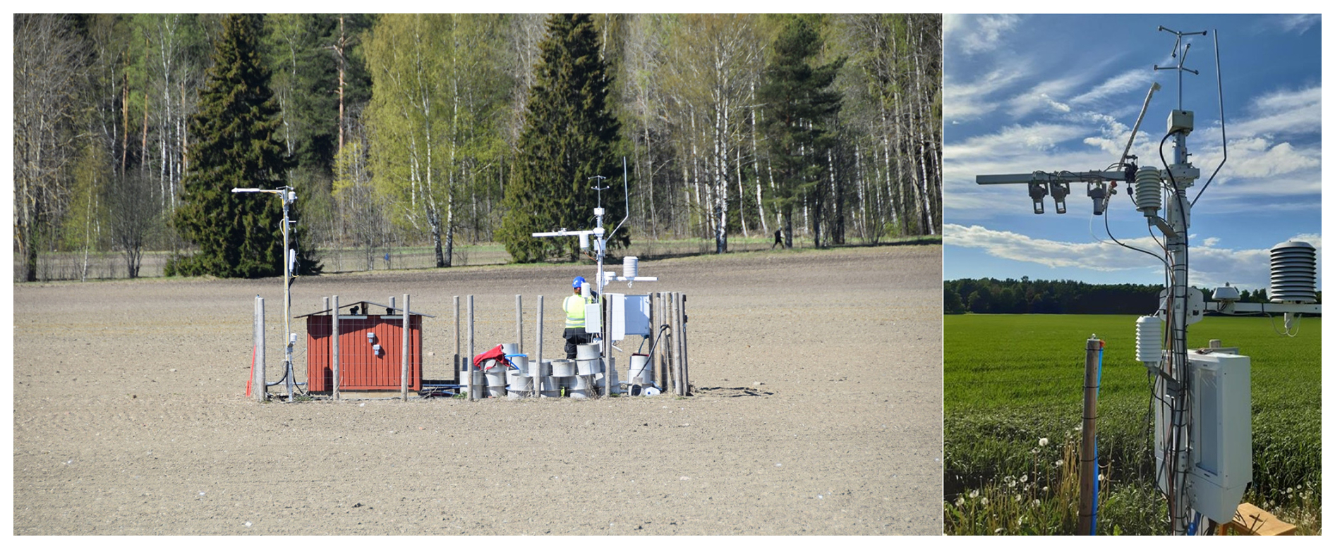
Figure 1 Left: Field installation of the reference (left tower) and the prototype (right tower) eddy covariance systems at Haltiala test site. Right: The prototype setup with Metek uSonic-3 anemometer.

During field measurements, the sensor performance was continuously monitored, and the instrument's autocalibration functionality was improved by several software updates. Initially, autocalibration was set to occur once every 30 min period. The main software update took place on 21 July 2022 around 10:00 UTC. Prior to this software upgrade, the auto-calibration was performed according to the following algorithm. The signals were measured with 5 Hz until temperature of the cell changed certain threshold (around 0.2 °C). Then autocalibration was applied by measuring a reference signal at 1 Hz for 1 s; after such calibration the CO₂ reading was adjusted to the reference signal. Then measurements continued again with 5 Hz frequency. With the software update on 21 July 2022, the signal jumps occurring with reference autocalibrations disappeared. The instruments software was modified to perform step-wise corrections for the drift between the calibrations against the reference signal using internal signals from instruments components. Continuous corrections to the signal virtually removed discontinuities in signal after each autocalibration.

Several additional software updates were done to further improve instrument's performance. The updates took place on 25 August 2022 at 10:30–11:00 UTC and 30 August 2022 between 12:30–13:10 UTC. The instrument was taken to Vaisala headquarters for maintenance on 8 September 2022 and returned to the field on 20 September 2022. The instrument received two more software updates on 27 October and 31 October 2022. At the end of the field experiments the prototype's calibration was tested in Vaisala's lab and no significant drifting was detected. Thus, the instrument did not suffer from signal drifting over 6 months period of field experiments. The maintenance breaks resulted in measurement gaps in particular in September to November months, see Figs. S3, S4. The impact of software updates on system performance is discussed in the following sections.

2.3 Data processing

The software update that most significantly impacted the sensor performance took place on 21 July at around 10:00 am UTC. Prior to this update, the autocalibration was performed in about 30 min intervals, and the sensor output readings experienced drifting, which, after periodic online calibration, resulted in signal jumps. The drift was primarily a function of temperature, but we could not establish well-behaving functional relationship for trend removal. Therefore, linear trend removal between the two consecutive calibrations was performed, ensuring that the readings prior to calibration matched those after calibration (see example in Fig. 2). After the software update on 21 July, these signal jumps during calibration were removed (see examples of raw signal time series in Fig. S2). Thus, well-designed autocalibration functionality appeared to be a critical feature of the prototype with the thermopile detector.

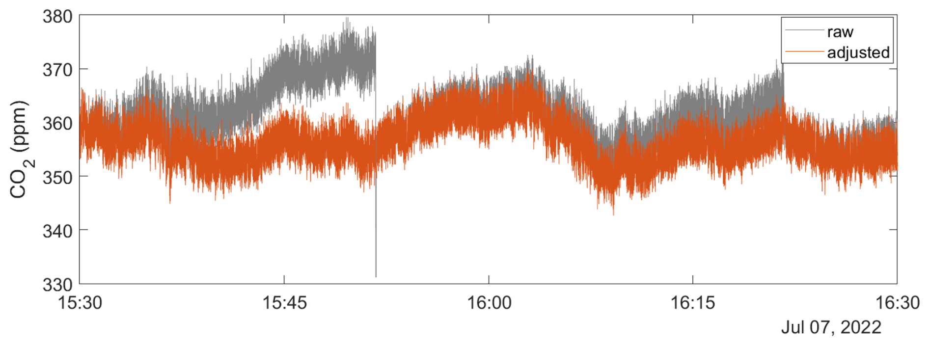
Figure 2 An example of turbulent CO₂ signal recorded by the prototype sensor before (raw, grey) and after calibration jump correction (adjusted, orange) prior to instrument's software update on 21 July 2022.

We calculated the turbulent fluxes using the EddyUH version 1.8 software (Mammarella et al., 2016). The fluxes were calculated for 30 min periods. Prior to flux calculation, we performed running mean high-pass filtering using a time constant of 150 s. This was to remove potential instrumental trends in the prototype sensor signal observed before the software update on 21 July 2022. For consistency, the Licor's signal was processed the same way. Prior to flux calculation, we performed standard data processing steps available in EddyUH, such as the raw data despiking, double rotation of the coordinate system for the velocity components and time-lag correction via cross-covariance maximization. For the prototype system, the lag time for the CO₂ signal varied from 0.4 to 0.8 s with a pronounced maximum at 0.6 s. The variation was smaller for the reference system, ranging between 0.2 and 0.4 s, with a maximum found at 0.3 s. Because the sampling lines were short, we did not expect the true lag time to vary, therefore, we fixed the lag times for CO₂ in further calculations at 0.6 and 0.3 s for the prototype and reference systems, respectively. For H₂O, we observed variation in lag time with relative humidity and used such dependence in the final flux calculation. Underestimation in the low-frequency spectral range was corrected using the theoretical transfer functions (Rannik and Vesala, 1999), while the high-frequency range was corrected via experimental transfer functions (Mammarella et al., 2009) for gas fluxes and theoretical transfer functions for momentum and sensible heat flux (Moncrieff et al., 1997). The density effect of water vapour fluctuations (Webb et al., 1980) was applied to the prototype instrument's 30 min average fluxes, while for the reference sensor, the correction was not relevant because of the internal conversion of wet mole fraction to dry one.

To quantify the frequency performance of the prototype system, we calculated the instrumental frequency response functions using good-quality observations from daytime in June and July 2022. The response times of the instruments were obtained by dividing the ensemble-averaged cospectrum of CO₂ by that of temperature and using least-squares fitting of the first-order frequency response function (e.g., Peltola et al., 2021). The instrumental noise values were estimated by using the method described in Lenschow et al. (2000).

3 Results and discussion

3.1 Evaluation of system characteristics

The ensemble-averaged power spectrum of the prototype system indicated the presence of noise at high frequencies in the CO₂ signal (Fig. 3a). Noise can be observed on the plot as the upward sloping power spectral densities (multiplied with frequency) starting from the normalised frequency around 0.5. The power spectrum of CO₂ for the reference system did not evidence any noise but rather minor damping of the signal at high frequencies when compared to the model curve. Compared to the CO₂ spectrum, the H₂O spectrum showed relatively less noise in the prototype sensor signal (Fig. 3c). The cospectra indicated damping of high-frequency fluctuations, particularly for H₂O (Fig. 3b, d). Note that the temperature cospectrum corresponded very well to the model cospectrum. Despite the short sampling line of the enclosed setup, damping of the H₂O signal is a common phenomenon attributable to relative humidity effects (Fratini et al., 2012).

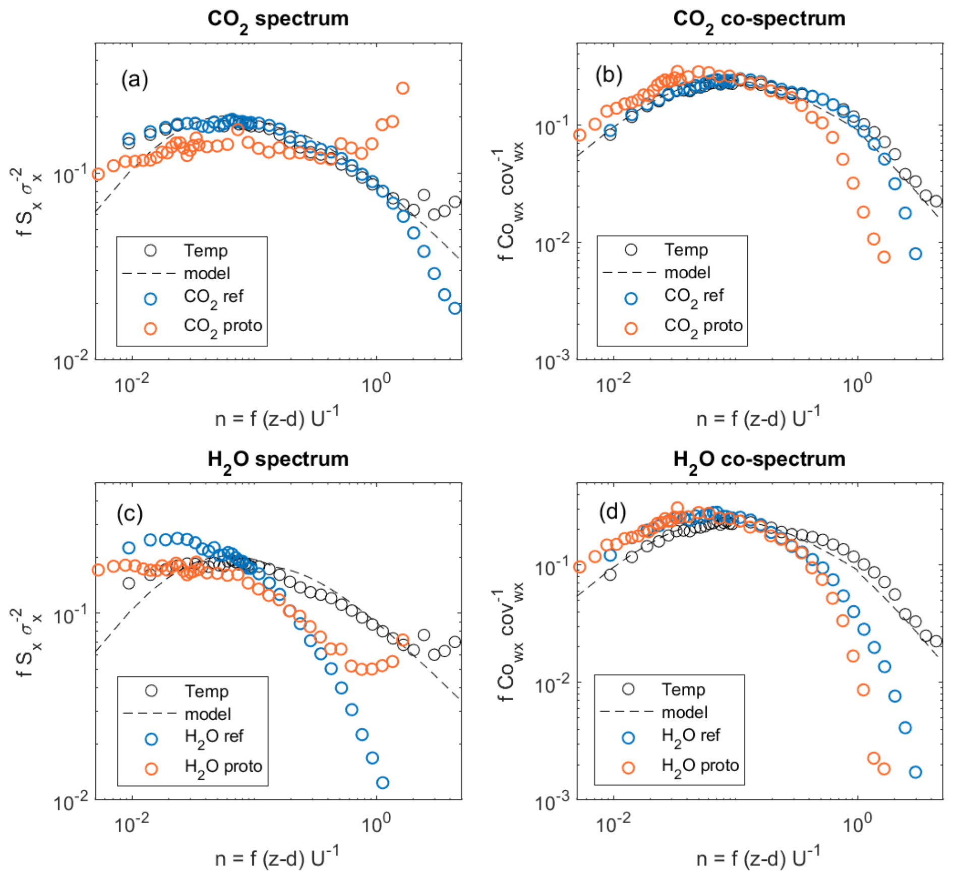
Figure 3 Ensemble average spectra and cospectra for CO₂ (a, b) and H₂O (c, d), averaged over the June–July (till 21 July 2022) period for the reference and prototype sensors. Unstable conditions were chosen (sensible heat flux >25 W m⁻²) with a limitation of wind speed from 2.5 to 3.5 m s⁻¹. The model curves for scalar spectra and cospectra correspond to formulations in Rannik and Vesala (1999). Temperature spectra were obtained using the reference system sonic anemometer measurements.

Using data from unstable conditions and limiting the wind speed interval for ensemble-averaging of cospectra resulted in relatively smooth curves for response time estimation (Fig. 4). The unstable conditions with the criterion for sensible heat flux >25 W m⁻²were chosen to use the measurements with higher flux magnitude in order to avoid division with erratic temperature co-spectral densities occurring with near-zero flux values and thus obtain more stable results. This is a common practice in response time estimation (e.g. Aubinet et al., 2012). The wind speed interval was used to limit the observations to similar conditions because the spectra generally shift on frequency axis with wind speed. The obtained result for CO₂ (first-order response time of 0.17–0.18 s) was in good correspondence with the response time obtained for the prototype instrument in laboratory measurements (0.2 s, not shown). The response time was very similar for both periods before and after the software updates on 21 July 2022. A similar analysis for the reference system using the LI7200RS analyser was performed, yielding the respective response time of 0.08 s.

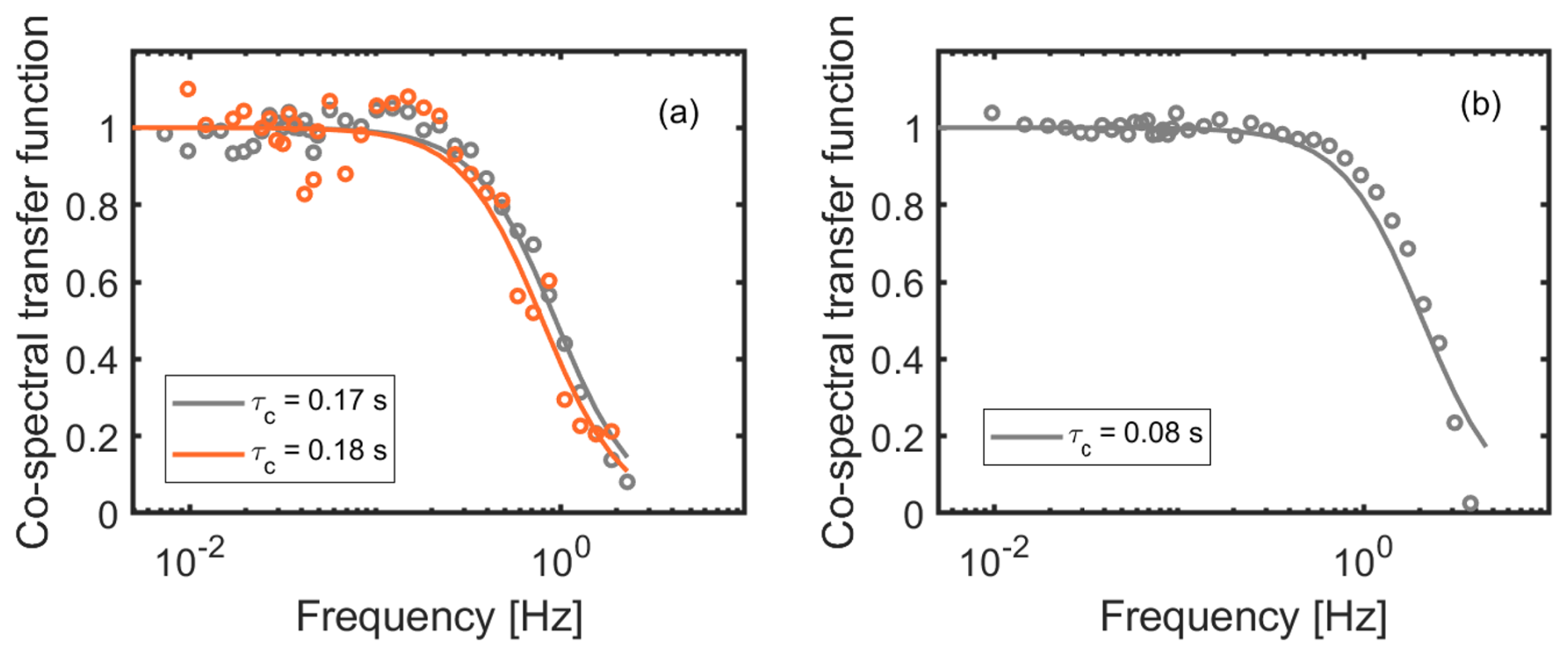
Figure 4 Frequency response functions estimated for (a) the prototype and (b) the reference systems. For transfer function estimation, unstable conditions were chosen (sensible heat flux >25 W m⁻²) with a limitation of wind speed from 2.5 to 3.5 m s⁻¹. The period was taken from the beginning of measurements till the software update on 21 July 2022 (grey curves and symbols). For the prototype system, the response function was estimated also from 21 July (after the software update; orange) till 31 July 2022.

The histograms of the noise values showed three distinct peaks, corresponding to different sub-periods of measurements and caused by the changes in the instrument's signal processing after firmware upgrades (Fig. 5). Initially, the noise level for CO₂ was between 2–2.5 ppm and for H₂O 0.1–0.2 ppth. An increase in signal noise level occurred on 21 July to about 3 ppm for CO₂ and 0.2–0.3 ppth for H₂O. At that stage the main challenge for the prototype was the signal jumps after autocalibrations. With the software upgrade the algorithm was improved at the cost of incorporating more noise from different hardware components. Thus, the signal stability, i.e. eliminating virtually the signal jumps after autocalibrations, was achieved at the cost of higher noise in signal.

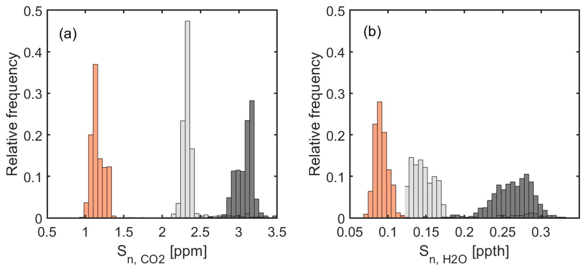
Figure 5 Histograms of the instrumental noise values (a) for CO₂ and (b) for H₂O determined by the method of Lenschow et al. (2000) for the prototype system. Observations from the beginning of measurements till the software update on 21 July are denoted with light grey, from then on till 20 September with dark grey and from then till the end of campaign with orange.

After maintenance and further improvements in software design, the noise level of the signal dropped to about 1.1 ppm level for CO₂ and to 0.1 ppth for H₂O after the software update on 20 September 2022. The signal noise of CO₂ around 1 ppm is an order of magnitude larger than the noise level of the reference LI7200RS instrument (reported to be 0.08 ppm at 5 Hz for CO₂). However, the noise level of 1 ppm corresponded roughly to flux random uncertainty of $\mathrm{5}\times {\mathrm{10}}^{-\mathrm{3}}$ ppm ms⁻¹ (approx. 0.24 µmol m⁻² s⁻¹) at 5 Hz sampling rate, assuming the averaging time 30 min and the representative value of the standard deviation of the vertical wind speed of 0.5 m s⁻¹.

Total flux random uncertainty is larger than the uncertainty originating from the instrumental noise; it is contributed also by stochastic nature of turbulence. In general, the random flux uncertainty is proportional to flux magnitude, being in the order of 10 % to 20 % of the value (Rannik et al., 2016). However, in near-zero exchange conditions the relative flux uncertainty (i.e. the random error divided by the flux magnitude) can be large. We calculated the flux random uncertainties of both systems according to the method by Finkelstein and Sims (2001) (Fig. S7). The histograms of the total random flux uncertainty for June–July period, when higher absolute fluxes prevailed, did not differ essentially for the prototype and the reference systems. However, during August-November period, the distributions for the reference system peaked at smaller values. This effect can be attributed to the impact of the higher signal noise of the prototype system. We estimated the random uncertainty of the CO₂ flux approximately 0.24 µmol m⁻² s⁻¹. This corresponded to the noise std of 1 ppm. However, during earlier phases of the field testing the noise level was higher roughly by a factor of 2. The noise level at initial phases of the field measurements introduced significant flux random uncertainty that limits accurate detection of small fluxes. The noise level obtained towards the end of the field experiments (after the software update on 20 September 2022) was relatively small and is a good compromise considering the cost target of the prototype. It is important also that random uncertainty does not impact accurate measurement of average fluxes over longer periods.

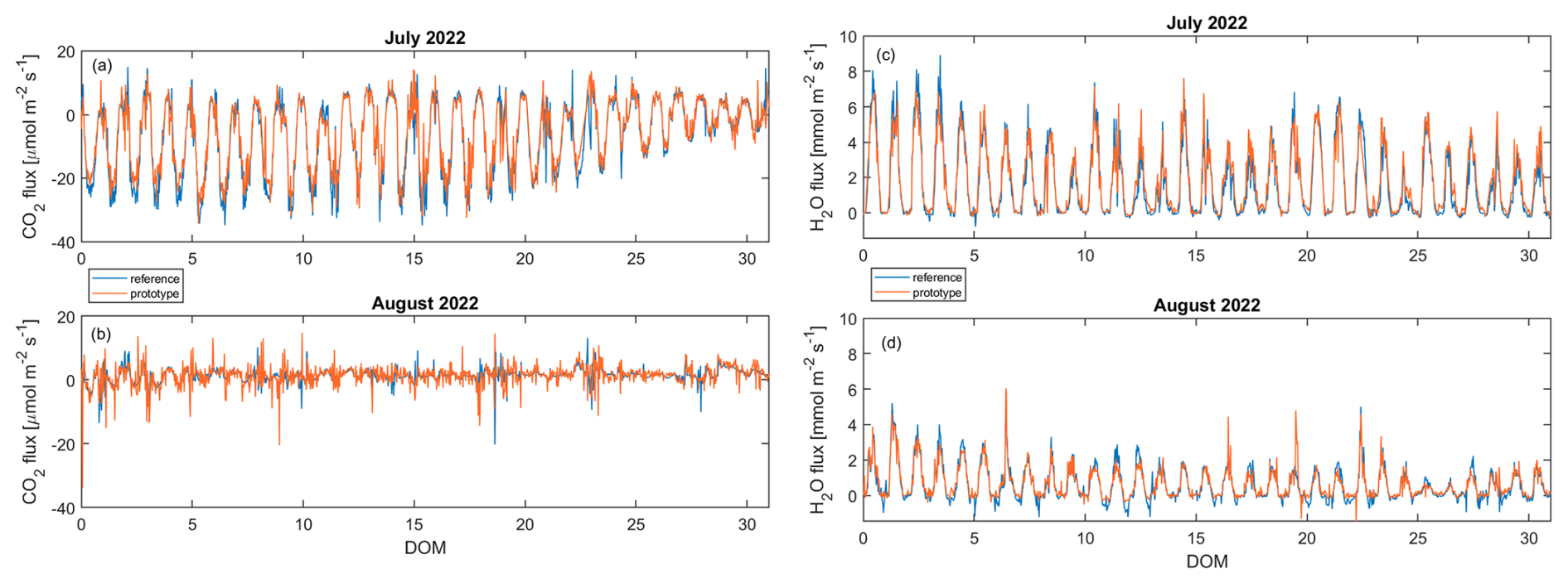
Figure 6 Time series of 30 min average fluxes measured by the prototype (orange) and the reference (blue) systems for July (a – CO₂ flux, b – H₂O flux) and August (c – CO₂ flux, d – H₂O flux). DOM denotes day of month.

3.2 Evaluation of average fluxes

The CO₂ fluxes had a strong diurnal variation in July and decreased in absolute values towards the end of August (Fig. 6a, b). Significant decrease in CO₂ fluxes took place earlier than the harvest; the transition from regular diurnal pattern to relatively irregular fluxes in the end of July was related to oat senescence. In July, the CO₂ fluxes ranged from about −30 µmol m⁻² s⁻¹ during the daytime to 10 µmol m⁻² s⁻¹ at night. In August, CO₂ fluxes were highly variable with a less clear diurnal pattern compared to those in July. This applied to measurements of both systems and was attributed to variability in fluxes during oat senescence and after the harvest rather than the (random) uncertainty in the measurements. The H₂O fluxes were more regular, including the diurnal variation in August (Fig. 6c, d). The H₂O fluxes ranged from about near-zero at night to +8 mmol m⁻² s⁻¹ during the daytime in the first half of July. The daily maximum H₂O flux values decreased to about 2 mmol m⁻² s⁻¹by the end of August.

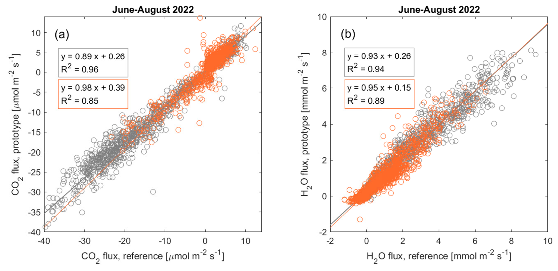
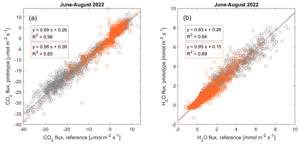
Figure 7 Comparison of 30 min average fluxes (a – CO₂, b – H₂O) of the prototype system with the reference system. The fitting parameters were obtained by using the orthogonal regression method. Grey and orange colours represent the measurements (and regressions statistics in respective bounding boxes) prior to and after the software update on 21 July 2022, respectively.

For further analysis of potential systematic differences between the systems, we plotted the half-hour average fluxes obtained from the prototype system against the reference system values, separating the period prior to and after the software update of the prototype sensor on 21 July 2022 (Fig. 7). The slopes obtained via the orthogonal regression procedure indicated underestimation of the flux magnitude by the prototype sensor compared to the reference system. However, the underestimation was reduced after the software update, as indicated by the regression statistics (see also Fig. 8). We note that the fluxes obtained by the two systems were well correlated with high values of the coefficient of determination (R²=0.85–0.96 for CO₂ fluxes and ∼0.90 for H₂O fluxes). The random errors of the CO₂ fluxes due to noise were around 0.2 to 0.3 µmol m⁻² s⁻¹ for the prototype system (Sect. 3.1), which is much lower than the scatter in Fig. 7a. The main source of the scatter can be attributed to the random uncertainty of fluxes due to stochastic nature of turbulence because the sensors, being separated horizontally by about 5 m distance, were not sampling exactly the same turbulence.

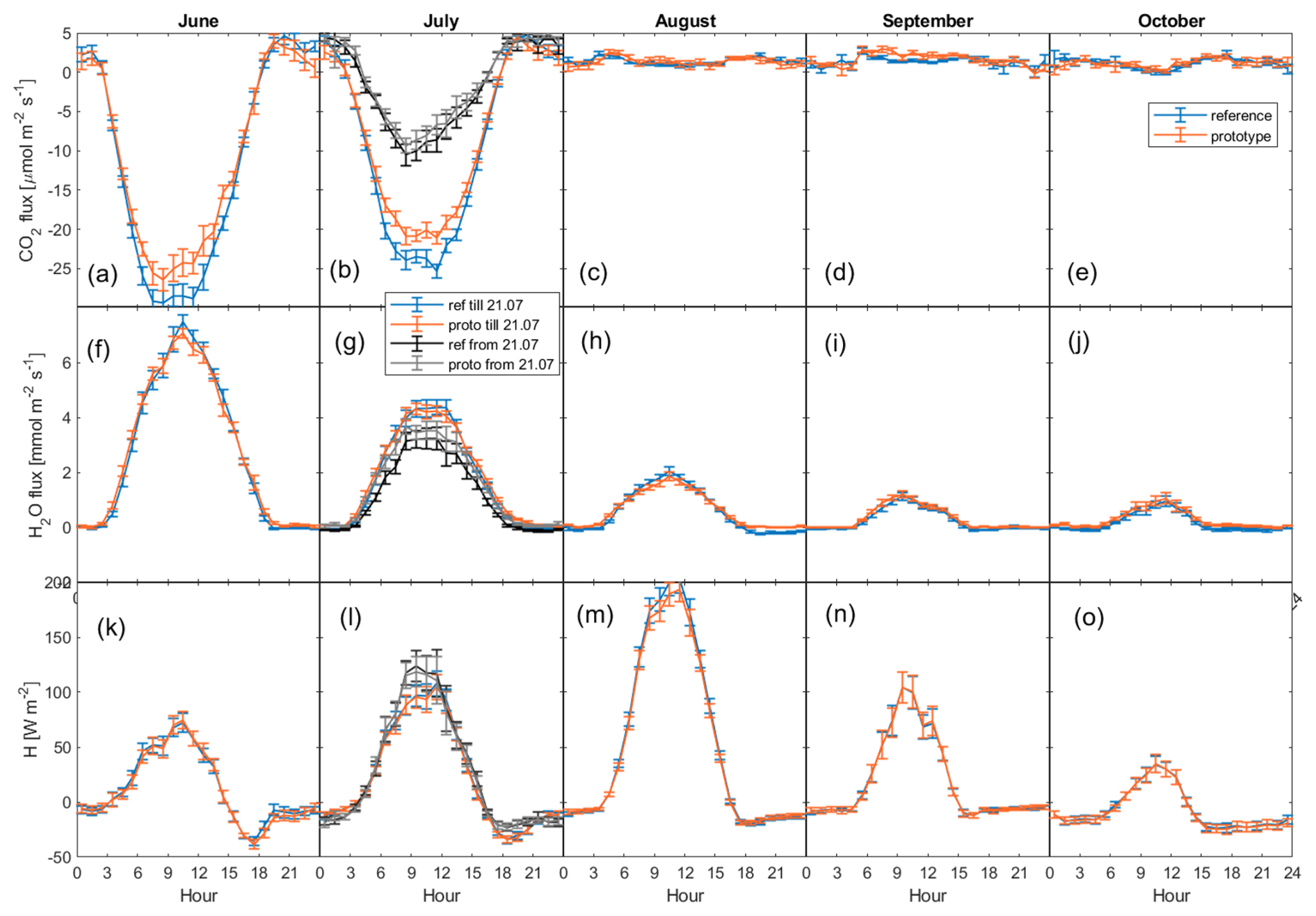
Figure 8 Monthly mean diurnal variation for CO₂ (a–e), H₂O (f–j) and sensible heat H (k–o) fluxes. In July (b, g, l), the period after the software update on 21 July 2022 is differentiated by black for the reference and grey for the prototype system. The error bars represent 1 standard error of the hourly bin averages. The magnitude of the fluxes after 21 July is significantly lower for CO₂ (b) due to decline in carbon assimilation rates towards the end of the month.

The diurnal variation of CO₂ fluxes was notably lower from August onwards compared to June and July (Fig. 8a–e), and the difference in CO₂ fluxes between the two systems was smaller after the software update on 21 July. Though small in magnitude, the CO₂ fluxes exhibit some difference during day-time hours in September month. In general, at 30 min time-averaging relatively large variation of fluxes occurs in the results of both systems (Fig. S3). We looked closer at the diurnal pattern in September (Fig. S8) and observed that two curves differ more than the errors at 95 % significance level only for a few hours, making it difficult to judge if they are truly different. A possible reason for the difference could be density fluctuations effects, if not properly accounted for by corrections. However, similar pattern is not observed in previous and following months and we have applied the same correction routines throughout the period. Also, we are not aware of system malfunctioning during this specific period of time. Thus, currently it remains unclear if the difference between the two system results is real and significant in September month.

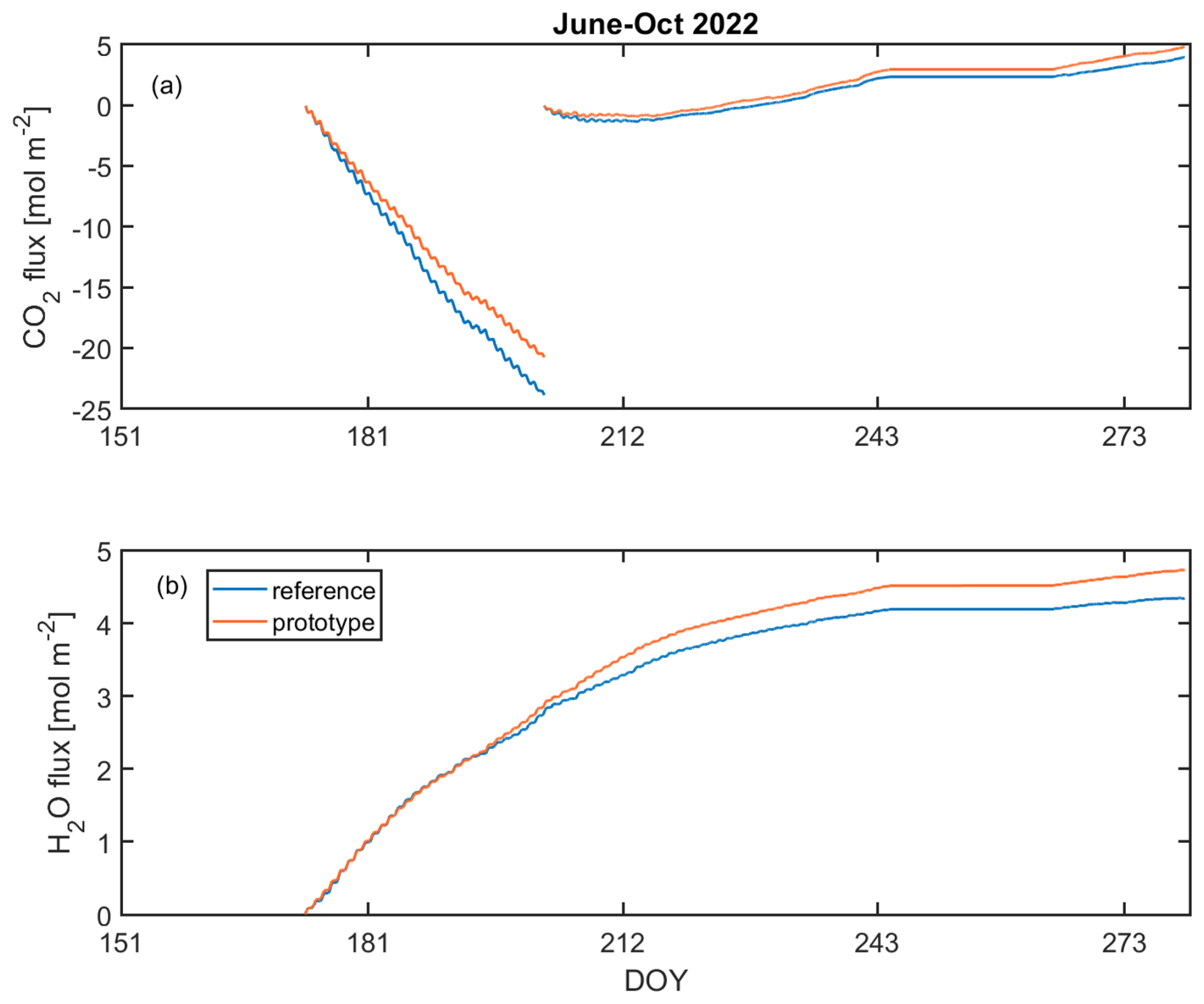
Figure 9 Cumulative fluxes for CO₂ (a) and H₂O (b) measured by the reference (blue) and the prototype (orange) systems. For CO₂, the cumulative value is reset to zero on 21 July 2022 (doy 202.4) due to a major software update. Cumulative curves were calculated over the periods when measurements from both systems were available; no gap-filling was done.

The magnitude of the H₂O fluxes between the systems was similar throughout the period (Fig. 8f–j). The sensible heat fluxes of the two systems were very close (Fig. 8k–o). In August, the H₂O fluxes were reduced and the sensible heat fluxes increased compared to July, indicating re-partitioning of the available energy after oat senescence in the end of July.

The cumulative fluxes diverged for CO₂ prior to the software update on 21 July (Fig. 9a) by 3.1 mol m⁻² (−13 %). After the update, the absolute difference was smaller. Starting from August, CO₂ fluxes were small, and from 21 July till the end of the field measurement period, the difference in cumulative flux was 0.8 mol m⁻² (+18 %). Considering the small values of the cumulative fluxes (4.0 mol m⁻² for the reference system), the difference between the results from the two systems can be considered small. The software update on 21 July improved the performance of the prototype sensor, resulting in a nearly production-ready analyser. For H₂O fluxes, the opposite was observed: until the software update, the difference between the cumulative values was small, after which the difference started to increase (Fig. 9b). The increased difference could be attributed to larger uncertainty in the high-frequency flux loss corrections at higher relative humidity conditions (for average diurnal variation of RH in each month see Fig. S5 and estimated system response time dependencies on RH see Fig. S6). Under such conditions, the overall system response is deteriorating for H₂O due to absorption/desorption of water in the sampling line. Despite determining the RH-dependent frequency response functions and applying the corrections respectively, which is a common practice (e.g. Mammarella et al., 2009), the difference in cumulative H₂O fluxes remained. The current study focused on analysing the CO₂ sensor's performance, so its ability to measure water fluxes with high accuracy was not prioritized in this analysis. The simultaneous measurement of H₂O concentration inside the sensor's sampling cell is a prerequisite for accurate CO₂ flux measurements due to density fluctuations created by variations in water concentration (Webb et al., 1980). However, the uncertainty introduced to H₂O fluxes of the reference system by spectral attenuation due to absorption/desorption effect in the sampling line does not impact the CO₂ flux detection accuracy of the system.

4 Summary and conclusions

A prototype of a LC high-response sensor was developed to measure CO₂ and H₂O concentrations, suitable for use in EC applications. We tested the enclosed-path setup in field conditions in summer and autumn 2022. The field setup included a separate reference measurement system containing commonly used instruments in scientific applications (Metek uSonic-3 Scientific sonic anemometer and Licor LI-7200 gas analyser). The LC prototype was developed by Vaisala Oyj in cooperation with the University of Helsinki. The sensor was designed to be inexpensive, easy-to-use and with minimized maintenance needs. The prototype sensor was aimed to compromise accuracy, reliability, and price. More specifically, the design was based on a thermopile detector operating at two channels for CO₂ and H₂O. The sensor was operating at 5 Hz measurement frequency and included internal temperature and pressure sensors to compensate for temperature, pressure and water vapour dilution. The prototype was equipped with an autocalibration feature for reference signal verification. The prototype analyser showed improving performance throughout the campaign, which was implemented with multiple software updates. When autocalibration was applied at 30 min intervals, the sensor using the early versions of the software suffered from signal drifting and jumps after applying autocalibration. The software update, performed approximately one month after the start of the field measurements (21 July 2022), fixed the issue with signal drifting.

The instrument's response time of 0.18 s for CO₂ allowed good accuracy of measurements with relatively small co-spectral corrections at field measurements over low vegetation. The lower sampling rate is not as important as the frequency response of the analyser. The frequency of signal sampling is related to the impact of disjunct sampling on calculated fluxes. If the measurements are instant values of the true signal, but sampling is done in intervals determined by sampling frequency, then calculated fluxes are not affected by systematic bias. The random uncertainty in the flux estimate, however, increases with decreasing sampling rate. The sampling induced uncertainty becomes important when the sampling interval is larger than the integral time scale of the flux time series (see, Bosveld and Beljaars, 2001; also Rinne et al., 2000; Turnipseed et al., 2009). Thus, reduction in sampling rate from 10 to 5 Hz has essentially no impact on calculated fluxes.

The noise level of the instrument was affected by the software changes and reached about 1 ppm for CO₂ and 0.1 ppth for H₂O by the end of the campaign in November 2022. Such a noise level would imply flux random uncertainty of about 0.2 µmol m⁻² s⁻¹ under typical observation conditions, much lower than the random uncertainty due to the stochastic nature of turbulence (can be a few µmol m⁻² s⁻¹, considering typical uncertainties from 10 % to 20 % of the flux magnitude, Rannik et al., 2016). The LC prototype achieved also good long-term accuracy of the CO₂ flux measurements and was capable of detecting the cumulative CO₂ flux with minimal systematic bias (after the software update on 21 July).

The achieved sensor performance showed high potential in balancing the substantially lower target price of currently commercially available instruments with the measurement accuracy. However, a deeper market analysis was carried out by Vaisala, and subsequently, the market in 2022 was not big enough for Vaisala's investments. As a result, Vaisala froze further development and productionization of the sensor.