The LOLland offshore Lidar EXperiment (LOLLEX): a novel observational approach for the study of wind farm flow and entrainment

Vertical momentum entrainment is driven by vertical shear and turbulent mixing and plays a key role in the recovery of wind turbine and wind-farm wakes, but remains poorly documented by field measurements. The LOLland offshore Lidar EXperiment (LOLLEX) campaign introduced a novel measurement approach to address this knowledge gap. The primary objective of this campaign was to develop a new atmospheric measurement strategy using Doppler wind lidar technology to better understand atmospheric conditions favourable to enhanced momentum entrainment inside and outside an offshore wind farm. LOLLEX was conducted from September 2022 to August 2023 in Denmark, in and around the Rødsand II wind farm, just south of the island of Lolland. During this campaign, two pulsed Doppler wind lidars, a scanning lidar (WindCube100S) and a lidar wind profiler (WindCubeV2), were deployed onboard a crew transfer vessel (CTV) commuting daily between the harbour and the Rødsand II offshore wind farm. Additionally, a scanning pulsed Doppler wind lidar (Halo Photonics) was mounted on a transformer platform north of the wind farm to perform range height indicator scans across the farm. Horizontal wind speed data were collected up to 300 m above the sea surface by the lidar wind profiler. The scanning lidar on the CTV collected data up to 2.5 km, alternating between the wind profiling mode and vertical stare mode. The latter scan operated at a sampling frequency of 1 Hz and along-beam spatial resolution of 10 m, allowing for the study of the turbulent vertical wind velocity component. The dataset includes several thousand hours of vertical scans. As a result of the moving vessel, many of the observations occurred inside or near the wind farm, providing insight into the near and far wakes of individual and multiple turbines. The potential and limitations of the new measurement strategy are illustrated using four case studies: (1) the observation of a Kelvin-Helmholtz instability above the wind farm, examined further in a companion paper; (2) turbulent mixing propagating downward from the top of the boundary layer; (3) internal atmospheric waves; and (4) wake characterisation inside the wind farm using the range-height indicator scans from the lidar deployed on the platform. This work demonstrates a novel methodology integrating remote sensing with a mobile offshore platform to measure turbulence at unprecedented altitudes. The dataset offers valuable data for wind energy research, boundary-layer meteorology, and further development of atmospheric measurement techniques.

1 Introduction

The European Union aims to commission at least 300 GW of offshore wind capacity by 2050, compared to 19 GW in 2023 (European Commission, 2023). Achieving this target requires a significant increase in the speed and scale of turbine deployment. Due to limited available space in the North and Baltic Seas, wind farms are being built in increasingly dense configurations, intensifying turbine interactions and wake losses (Borgers et al., 2025). Wake losses refer to the reduction in power output caused by turbine interactions within a wind farm or between farms. Within a farm, downstream turbines operate in the slower, more turbulent air generated by upstream turbines. These wake effects reduce annual energy production (AEP), complicate farm layout design, and thus increase the levelized cost of energy (LCOE) (Akhtar et al., 2021; Pryor et al., 2021; Minz et al., 2025). They may also pose legal challenges (Finserås et al., 2024) and affect electricity market integration (Kenis et al., 2023). Coupled mesoscale-microscale wind models and analytical wake models have been widely used to quantify wake losses, assess wake extent, and support AEP and LCOE optimisation (Sanz Rodrigo et al., 2017; Pryor et al., 2021; Haupt et al., 2023; Wang et al., 2024).

Wake recovery is governed by momentum entrainment, encompassing both vertical and lateral contributions, and referring to the turbulent transport of momentum into the wake. This process replenishes the kinetic energy extracted by turbines and is therefore a key mechanism controlling wake recovery. Following van der Laan et al. (2023), momentum entrainment can be expressed as the divergence of the Reynolds shear stresses. Under this definition, wake recovery is driven mainly by the lateral and vertical gradients of these stresses.

Momentum entrainment has been quantified using computational fluid dynamics and associated bulk formulations based on velocity differences across an interface and entrainment coefficients (Bempedelis et al., 2023), with further support from Large Eddy Simulations and limited field data (Calaf et al., 2010; Luzzatto-Fegiz and Caulfield, 2018). This process is sustained by turbulent transport from the atmospheric boundary layer (ABL) into the internal boundary layer (IBL), which replenishes the kinetic energy within the farm (Frandsen, 1992; Abkar and Porté-Agel, 2013; Porté-Agel et al., 2020; Meneveau, 2019; Krishnamurthy et al., 2025). However, the quantification of the momentum entrainment from field measurements, particularly above offshore wind farms, remains scarce (Meneveau, 2019; Giebel et al., 2021; Syed et al., 2023; Krishnamurthy et al., 2025).

Commercial Doppler wind lidars (DWLs) have increasingly been used in wind energy since the 2000s (Peña et al., 2013; Slinger and Harris, 2013; Gottschall et al., 2017). To the authors' knowledge, however, DWLs have seldom been used to observe and quantify momentum entrainment in the ABL. Lidar wind profilers are primarily used to measure mean wind speed profiles in the first 300 m above the surface (Hasager et al., 2008). In contrast, long-range scanning lidars can provide additional insights into mean and turbulent flow characteristics with ranges extending several kilometres (Lothon et al., 2006; Cheynet et al., 2017b). The scanning DWLs can operate in various modes, including Doppler beam swinging (DBS) for wind profiling, range-height indicator (RHI), plan-position indicator (PPI), and fixed line-of-sight scans. Most offshore DWLs are deployed on fixed offshore infrastructure such as substations or platforms supporting bottom-fixed meteorological masts (Krishnamurthy et al., 2017), which limits spatial coverage. Although lidar wind profilers have been deployed on floating buoys or vessels (Gottschall et al., 2017, 2018; Kelberlau and Mann, 2022; Rubio et al., 2022), they are often used to measure the mean wind speed and direction only, and scanning lidars are rarely deployed on vessels or buoys.

To address this gap, we present a new measurement strategy using two DWLs mounted on a crew transfer vessel (CTV). This mobile setup allows flexible positioning near or inside the wind farm, providing wind speed profiles and high-resolution vertical velocity measurements. This combination offers the possibility to study atmospheric boundary layer physics, including wake recovery and vertical momentum entrainment, inside and above offshore wind farms.

This study provides an overview of the LOLLEX campaign, conducted from September 2022 to August 2023 at the Rødsand II wind farm in Denmark and presents the collected dataset through selected case studies. Motion-compensated DWL measurements from moving platforms have been demonstrated in recent studies (e.g.  Duscha et al., 2022; Pichugina et al., 2026). The LOLLEX campaign constitutes an independent offshore implementation in which two pulsed DWLs operated simultaneously on a routinely transiting CTV. This allowed repeated in-motion profiling of wind speed and turbulence within and around an active offshore wind farm to investigate vertical momentum entrainment.

This paper starts with the campaign description in Sect. 2, including site characterisation, instrumentation and the selected lidar measurement setup. Section 3 then describes the methods used in this study, including data processing and quality control, and motion correction. Furthermore, Sect. 4 summarises the collected dataset and its availability. Section 5 presents the motion correction results for the overall campaign and four case studies: three based on the lidars mounted on the CTV and one from the scanning lidar installed on the transformer platform. Finally, Sect. 6 discusses the potential and limitations of the current measurement setup in comparison with DWLs deployed on fixed platforms or buoys.

2 Campaign description

The LOLLEX measurement campaign was carried out between September 2022 and August 2023 as a collaborative effort between the MSCA-ITN project Train²Wind, funded by the EU Horizon 2020 scheme, and the RWE group. The main goal of Train²Wind was to advance the understanding of entrainment processes relevant for large offshore wind farms. The choice of Rødsand II was mainly guided by logistical considerations, such as the accessibility of a well-suited CTV and the well-positioned transformer platform. Its proximity to the land was an additional factor, as the initial experiment plan also included considerable complementary measurement activities using various uncrewed aerial systems. However, most of these activities could not be performed as intended due to regulatory constraints.

2.1 Experiment site

The Rødsand II wind farm (54.5799° N, 11.8903° E), in operation since 2010, is located in the shallow waters of the Baltic Sea, south of the island of Lolland (Fig. 1). The farm consists of 90 Siemens SWT–2.3–93 turbines, each with a nominal capacity of 2.3 MW, a hub height of 68.5 m, and a rotor diameter (D) of 93 m. The farm is arranged in five curved rows of 18 turbines each, with inter-turbine spacing ranging between 5D and 8D (see also the bottom panel of Fig. 4). Approximately 3 km to the east lies the Nysted wind farm, commissioned in 2003, comprising 72 Bonus 2.3 MW turbines with a spacing ranging from 6D to 10D. The nearest landmass, the island of Lolland, is characterised by low-lying, flat terrain with sandy beaches, coastal dunes, agricultural fields, small settlements, and patches of forest. The region experiences high average wind speeds of about 9.6 m s⁻¹ at 100 m, predominantly from the west to the south-west, influenced by weather systems passing over the North Sea and Baltic Sea (Davis et al., 2023, see also https://globalwindatlas.info/en/, last access: 22 September 2026).

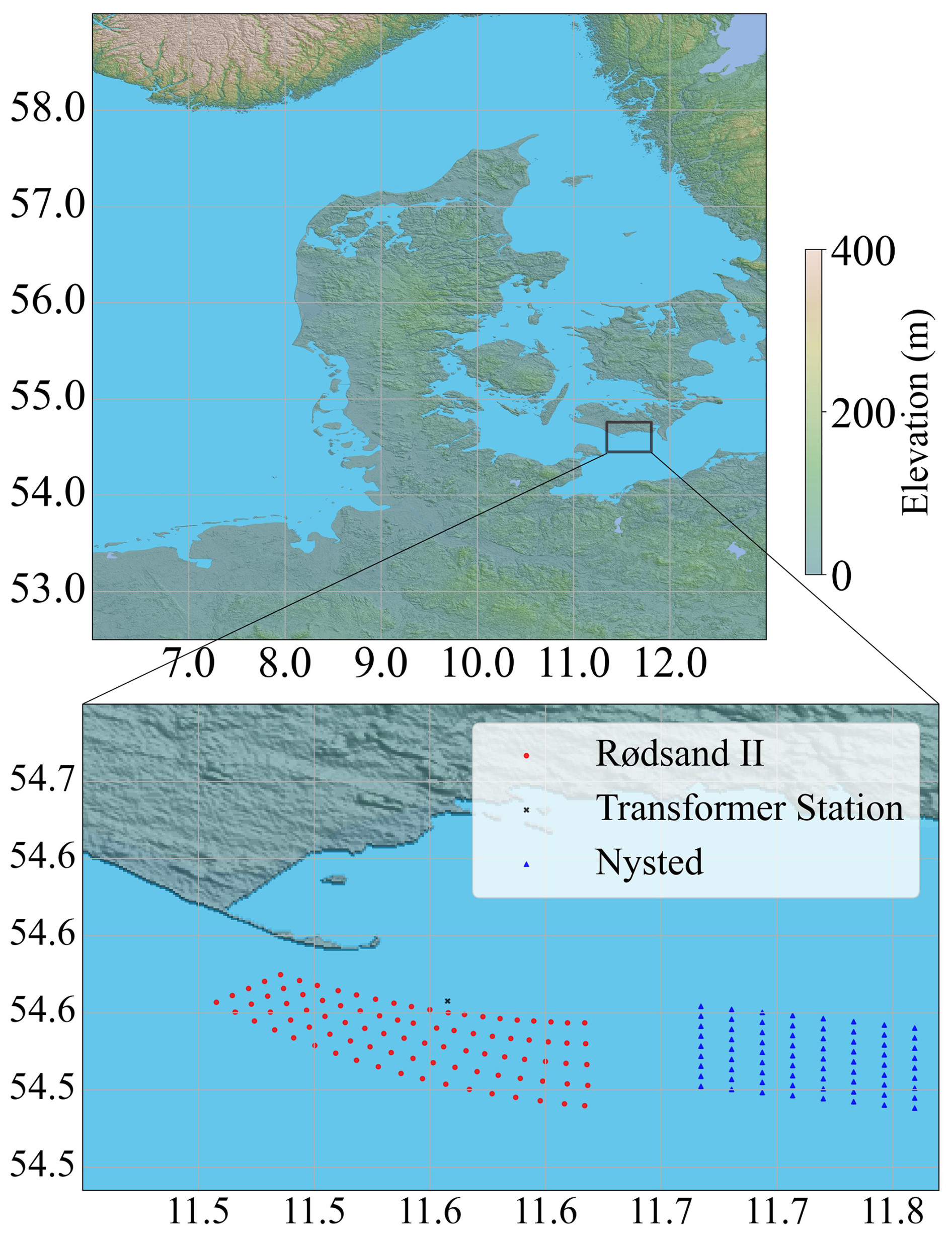
Figure 1 The location of the Rødsand II wind farm in the shallow waters of the Baltic Sea, south of Denmark, near the island of Lolland. This wind farm is located adjacent to the Nysted wind farm. This map was created using Rasterio (an open-source Python library by MapBox) version 1.4.2 (https://rasterio.readthedocs.io/, last access: 22 September 2026). The digital elevation model was obtained from SRTM data V4, provided by the International Centre for Tropical Agriculture (CIAT), available at https://srtm.csi.cgiar.org (last access: 22 September 2026). SRTM v4 DEM data © CIAT/CGIAR-CSI, CC BY 4.0 (Jarvis et al., 2008).

During more than a decade, Rødsand II and Nysted have been used for studies on the interaction between atmospheric flow and wind farm arrays, in particular wind turbine wakes and wind farm interactions, also called cluster effect (Hansen et al., 2015). Previous studies focusing on wake loss for these two farms used simulations alone (Nygaard and Hansen, 2016), combined SCADA data and numerical simulations (Hansen et al., 2015; Fischereit et al., 2022) or simulation and mast-based measurements (Cleve et al., 2009).

There have, however, been only a few measurement campaigns that have focused on wake flow characteristics and the structure of the ABL above Rødsand II. In 2013–2014, a scanning lidar campaign under the lead of the Carbon Trust Offshore Wind Accelerator program was performed. It was aimed at investigating wake flow and boundary layer dynamics at Rødsand II. Only a limited portion of the results from this campaign has, however, been openly published (Borbón, 2019).

The LOLLEX campaign builds on these foundations and introduces several novel and complementary elements: a long-range scanning lidar deployed on the offshore transformer platform north of the wind farm and a dual scanning-profiling lidar setup mounted on a CTV as an observational platform of opportunity.

To complement the lidar data, high-resolution mesoscale wind speed data from the 3 km Norwegian Hindcast Archive (NORA3) (Haakenstad et al., 2021) were used. NORA3 is a state-of-the-art hindcast dataset produced by dynamically downscaling ERA5 reanalysis data (Hersbach et al., 2020). It provides hourly wind conditions over Northern Europe at a horizontal resolution of 3 km. The dataset has been validated against both in-situ observations (Solbrekke et al., 2021) and remote sensing data (Cheynet et al., 2025), demonstrating excellent performance in coastal and offshore environments.

During the LOLLEX campaign, a specific subset of the NORA3 database, containing wind speed data at seven vertical levels from 10 to 750 m, was used in combination with the lidar observations above the wind farm, as shown in Malekmohammadi et al. (2025). It was also used to complement the Range Height Indicator (RHI) scans from the lidar installed on the transformer platform (see Sect. 5).

2.2 Instrumentation

The backbone of the campaign was the installation of two DWLs onboard a CTV serving the Rødsand II wind farm, using it as an observational platform of opportunity. This mobile measurement set-up over several months was complemented by the shorter fixed deployment of an additional scanning lidar system on the transformer platform of the wind farm.

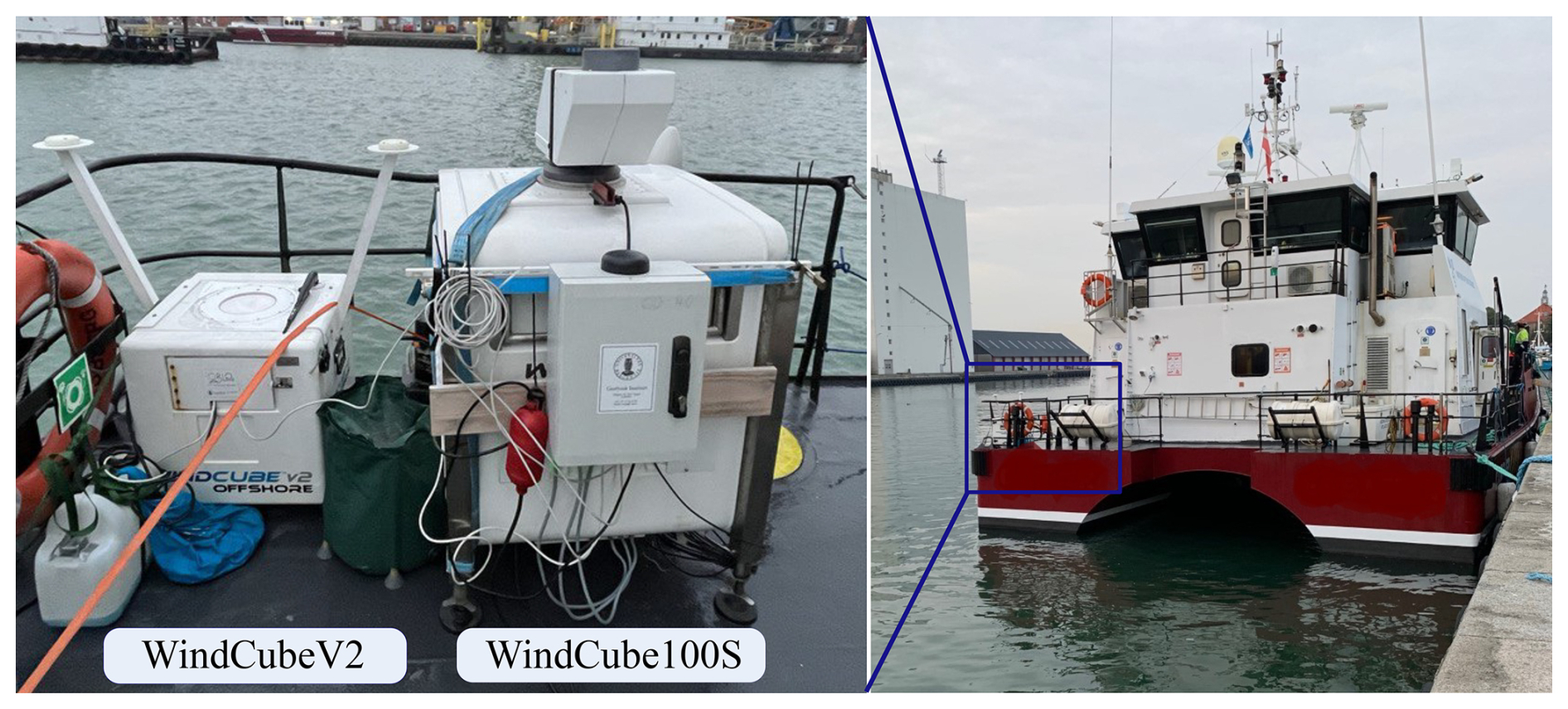
Figure 2 Location of the WindCubeV2 and WindCube100S lidars mounted on the stern of the CTV. Azimuth angles were defined relative to the vessel's heading and corrected using GPS true heading from the IMU.

2.2.1 Lidar deployment on the CTV

In September 2022, the WindCubeV2 was installed on the stern of a 27 m long and 10 m wide CTV, which operated nearly daily between Rødby harbour and the Rødsand II offshore wind farm for the transport of personnel and material for maintenance purposes. The vessel operations are typically performed between 07:00 am and 07:00 pm, providing up to 12 h of wind field observations offshore, inside and around the farm. The lidar was installed with its east-facing side oriented toward the bow (see Fig. 2). From September 2022 to January 2023 the WindCube100S remained onshore, deployed in the parking area of RWE Wind Services Denmark at the quay in Rødbyhavn, allowing for night-time co-located measurements while the CTV was in harbour. The second phase of the LOLLEX campaign started in the last week of January 2023 with the installation of the WindCube100S on the CTV side-by-side with the WindCubeV2 (Fig. 2).

The WindCubeV2 measured wind speed and direction at 11 heights, ranging from 40 to 290 m, at a sampling frequency of 0.25 Hz. The system included a motion sensor and an Inertial Measurement Unit (IMU) that recorded attitude data at 10 Hz. The IMU tracked pitch, roll, yaw, and translational velocities in the x, y, and z directions, as well as GPS coordinates (latitude, longitude, altitude). The IMU also provided the vessel's heading using GPS True Heading. In the WindCubeV2, the IMU is part of an integrated unit linked to a differential GPS (GNSS). This configuration indicates that the reported position and attitude are not based on a purely inertial solution; instead, the inertial measurements are constrained by GPS, which limits the accumulation of low-frequency drift over time.

The WindCube100S is a scanning lidar with a scanner head possessing hemispherical scanning capability. The instrument operated on a 30 min scan cycle alternating between two modes: 5 min of DBS for wind profiling (left panel in Fig. 3) and 25 min of vertical velocity measurements in vertical stare mode (right panel in Fig. 3). The 5 min DBS duration, shorter than the 10 min averaging period commonly used in the wind industry, was selected to maximise the duration of vertical stare measurements used for turbulence and entrainment analysis. A comparison between 5 and 10 min averages derived from the WindCubeV2 lidar showed only minor differences in mean wind speed, apart from the expected increase in statistical uncertainty for the shorter averaging period.

In vertical stare mode, which corresponds to a line-of-sight (LOS) configuration with an elevation angle of φ= 90°, the lidar operated at a sampling frequency of 1 Hz at ranges between 50 and about 2500 m. In DBS mode, the lidar operated using a five-beam scanning configuration. Four oblique beams were sequentially emitted at an elevation angle of φ= 75° and azimuth angles of α= (0, 90, 180, 270°), followed by a vertically pointing beam with an elevation angle of φ= 90° at ranges between 50 m and about 2500 m (Fig. 3). During each 5 min DBS period, approximately 80 individual samples were collected, corresponding to an effective sampling frequency of 0.3 Hz. In wind profiling mode, the lidar retrieves wind speed and wind direction. Both instantaneous estimates and 5 min time-averaged products were computed in post-processing (see Sect. 3.3).

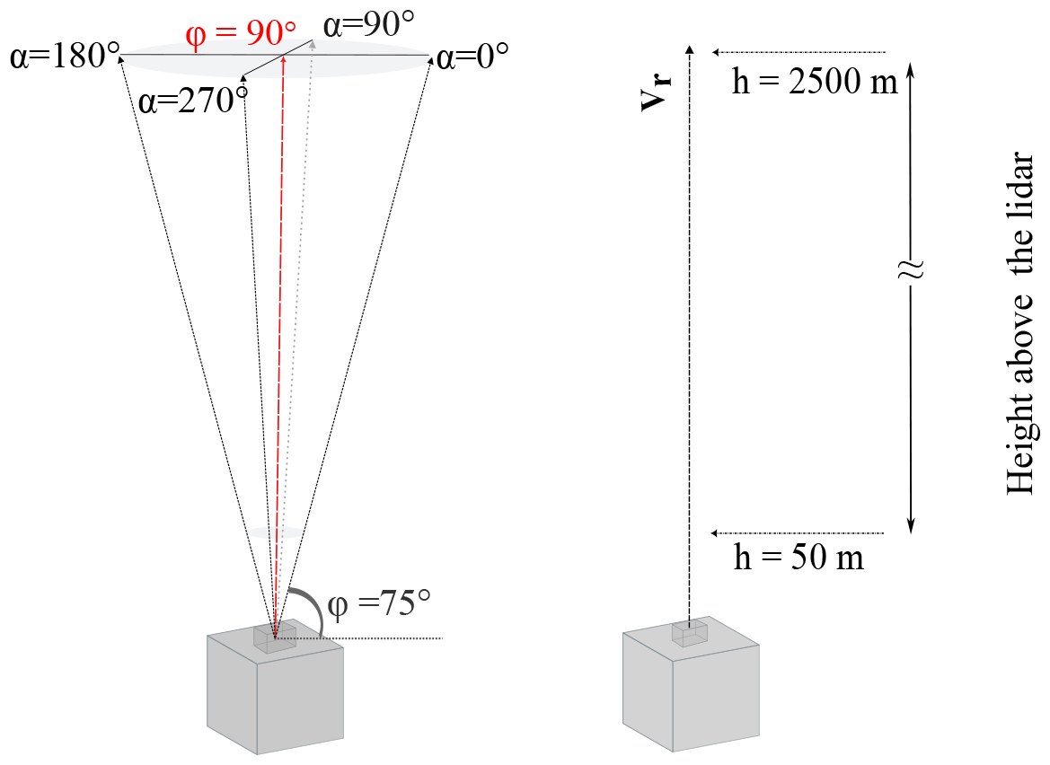
Figure 3 Schematic of the WindCube100S scanning configurations used in this study. Left: five-beam DBS mode with inclined beam with the elevation angle (φ) of 75° and four azimuth angles (α), plus a vertical beam with the elevation angle (φ) of 90°. Right: vertical stare mode with the elevation angle (φ) of 90°.

2.2.2 Scanning lidar on transformer platform

To complement the ship-based measurements, a Halo Photonics by Lumibird StreamLine XR+ scanning Doppler lidar was deployed on the transformer platform located north of the wind farm from April to August 2023 (Fig. 4). The lidar was mounted at a height of approximately 25 m above sea level. It operated in RHI mode at a fixed azimuth angle of 206°, elevation angles increasing from −1 to +10°, and a range gate length of 12 m. With an angular speed of 1° s⁻¹ and an accumulation time of 0.5 s, a full RHI scan including fast return, took about 16 s.

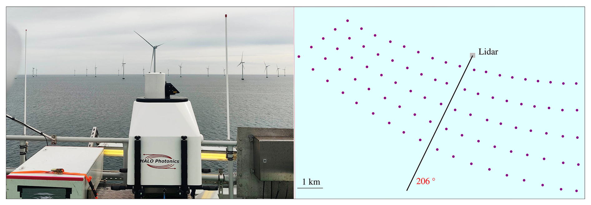
Figure 4 Left panel: The scanning lidar Halo Photonics by Lumibird StreamLine XR+ installed on the substation (view toward South). Right panel: Sketch of the lidar line of sight (top view) with an azimuth angle of 206° and a scanning range of 6 km.

The scan sector extended from north to south across the wind farm. This allowed for the observation of wake propagation in the plane where the ship-based lidars travelled, facilitating the interpretation of those measurements as well as providing a continuous data set for studies of intra-farm turbulence. For wind directions approximately perpendicular to the lidar's line of sight, the nearest turbine was about 0.7 km away, and at that location the lidar beam intersected the rotor area around 20 times per scan, yielding a vertical resolution of approximately 6 m within the wake. The farthest turbine was located 3.8 km away, where the beam crossed the rotor area only three times per scan direction, resulting in a vertical resolution of about 38 m (Fig. 5). At longer distances, the decrease in vertical resolution reduced the accuracy of wake characterisation. The exact wake position and shape also varied with the wind direction and the operating conditions of the turbine, such as yaw misalignment and rotor tilt.

The RHI scan was selected to support the campaign's focus on vertical momentum entrainment. The choice of only one RHI scan was made with the purpose of providing sufficient statistics of continuous data in the targeted plane. Nevertheless, since a DWL only measures the LOS speed component, this configuration imposes some limitations on the wind directions for which the wakes can be observed. In most cases, wake signatures are detectable, except when the wake's lateral cross-section is exactly aligned with the RHI plane. In that case, the lidar cannot detect any component of the axial wake flow.

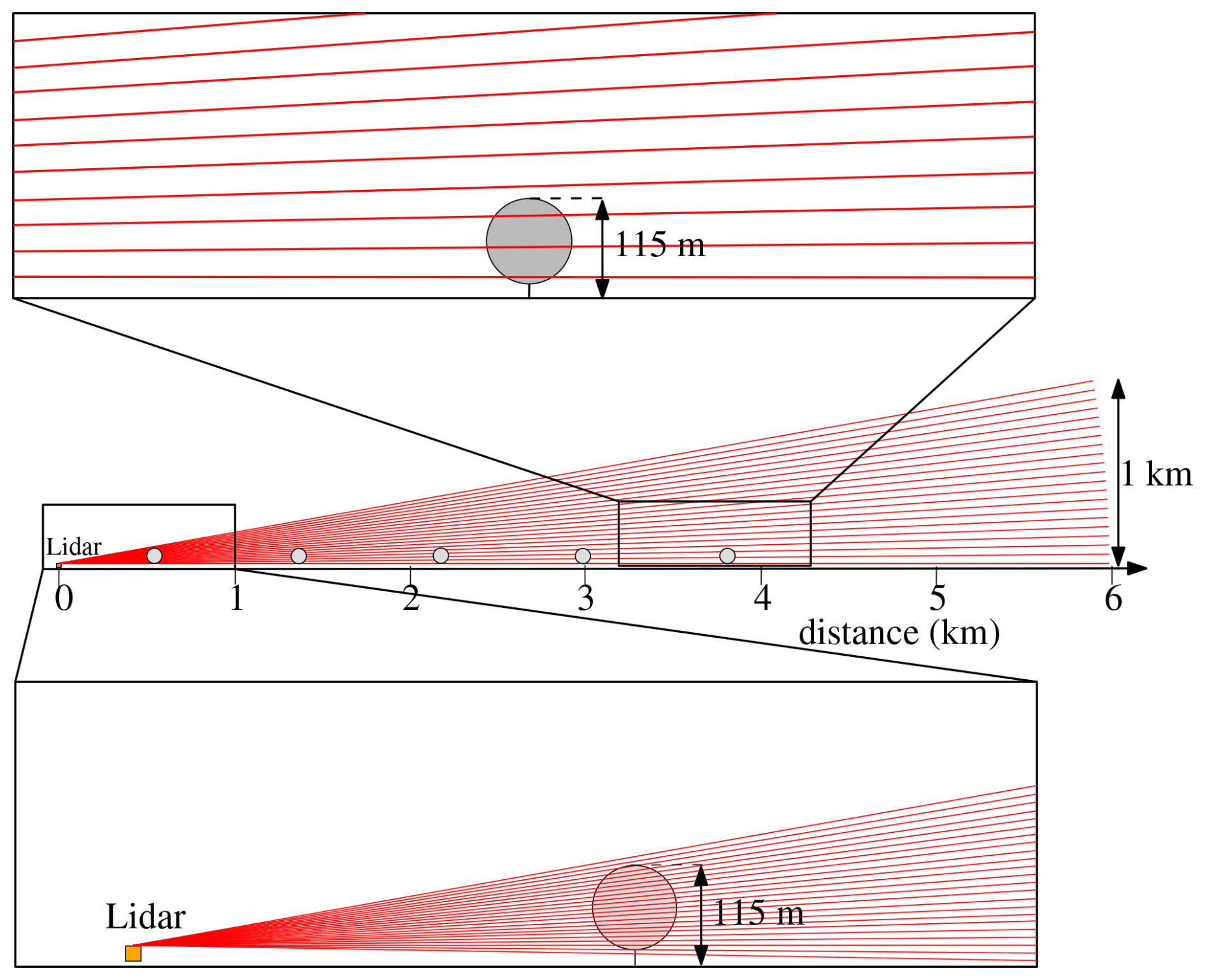
Figure 5 Sketch of an RHI scan in the case where the wake direction is perpendicular to the azimuth. The turbine rotors are indicated as grey circles. The inset sketches the lidar beams crossing the rotor plane at different distances: at around 3.8 km (top inset) and 0.7 km (bottom inset) from the lidar.

3 Methods

This section describes the motion correction algorithm applied to the data collected by the lidar wind profiler WindCubeV2 deployed on the CTV. It also introduces a new method to correct for the static tilt angle error of the WindCube100S in vertical stare mode. Finally, it details the pre-processing steps for filtering the data and dismissing the erroneous data.

3.1 Data processing and quality control

The WindCube100S occasionally produced short or incomplete scans when deployed on the vessel, likely due to its sensitivity to rapid translation and acceleration. This can be attributed to its mechanically rotating scanning head for beam steering, in contrast to the WindCubeV2 Offshore, which operates without moving parts and is designed for dynamic buoy deployments. For the vertical staring mode conducted between 25 January and 28 August 2023 (approximately 9900 scans), 65 % of the WindCube100S scans were flagged as incomplete (scan duration <10 min) and excluded, while 30 % achieved the full 25 min duration.

All lidar measurements were subjected to a two-step quality control procedure to ensure high-quality data for further analysis. In the first step, a signal-quality filtering was applied using the Carrier-to-Noise Ratio (CNR), which is provided by both the WindCubeV2 and WindCube100S. A fixed CNR threshold was applied at each time and range gate to remove low signal-to-noise measurements. Following earlier studies (Kumer et al., 2014; Cheynet et al., 2017b; Suomi et al., 2017), thresholds of −24 dB for the WindCubeV2 and −27 dB for the WindCube100S were used.

In the second step, statistical outliers were removed using a moving median absolute deviation (MAD) filter with 3 MADs away from the median, following Starkenburg et al. (2016) and Leys et al. (2013), to eliminate spurious values that passed the CNR threshold but were inconsistent with local temporal variability. After signal-quality filtering and statistical outlier removal, data availability was range-dependent. That is, within a given scan, valid data could be retained at lower ranges while being filtered out at higher ranges. Therefore, data availability could not be represented by a single campaign-wide percentage. After quality control, motion correction was applied to the WindCubeV2 data and to the DBS-mode scans of the WindCube100S, as described in Sect. 3.2. Unless otherwise stated, all results presented in this manuscript are based on motion-corrected wind speed data.

Following Päschke et al. (2015), a signal-to-noise ratio (SNR) threshold of −20 dB is commonly recommended for radial velocity data from the Halo Photonics StreamLine XR+. In the present case, this threshold appeared overly conservative. The lidar data were used solely for mean wind speed estimation, and the beam was frequently oriented at angles close to 90° relative to the mean wind direction, resulting in generally low SNR values. In addition, the SNR was originally provided on a linear scale, with a substantial fraction of values being negative, preventing a consistent conversion to dB.

For case study 4, a moderate correlation ($\mathit{\rho }\approx -\mathrm{0.63}$) was found between the SNR and $|v_{\mathrm{r}}-v_{\mathrm{0}}|$, where v_r is the along-beam (radial) velocity and v₀ denotes the most probable radial velocity. However, substantial overlap between low- and high-deviation data across the SNR range indicates that SNR alone is not a reliable indicator of data quality. Consequently, no SNR-based filtering was applied. Radial velocity data were first filtered to remove implausible values by discarding samples with $\left|v_{\mathrm{r}}\right|>\mathrm{30}\mathrm{m}{\mathrm{s}}^{-\mathrm{1}}$. The most probable radial velocity v₀ was then estimated as the mode of the v_r distribution. Only samples satisfying $|v_{\mathrm{r}}-v_{\mathrm{0}}|<k\mathrm{MoAD}$ were retained, where $\mathrm{MoAD}=\mathrm{median}\left(|v_{\mathrm{r}}-v_{\mathrm{0}}|\right)$ denotes the median absolute deviation about the modal radial velocity v₀, and k=3 is a dimensionless threshold parameter.

The ABL top is inferred from vertical-stare lidar measurements using both CNR and σ_w profiles when these diagnostics are well defined. Aerosol- and backscatter-based methods are commonly used to estimate ABL height from lidar and ceilometer observations (Caicedo et al., 2017; Vivone et al., 2021), but the resulting height should be interpreted as a proxy rather than as an exact thermodynamic inversion height. This is particularly important in cloud-topped conditions, where cloud droplets may dominate the CNR signal and the CNR maximum may correspond to a cloud-related backscatter feature that is not necessarily collocated with the actual ABL top. When a distinct local minimum is visible in the vertical profile of σ_w, it is used as an additional turbulence-based indicator of ABL depth, following previous Doppler-lidar studies based on vertical velocity variance profiles: Tucker et al. (2009) used the altitude where ${\mathit{\sigma }}_w^{\mathrm{2}}$ drops below an empirical turbulence threshold, whereas Puccioni et al. (2024) used the minimum of ${\mathit{\sigma }}_w^{\mathrm{2}}$ under stable conditions.

3.2 Motion correction for DBS scans

A lidar wind profiler mounted on a moving platform, such as a buoy or ship, is subject to six degrees of freedom (DOF) of motion. These include translational movements, such as surge, sway, and heave along the platform’s x, y, and z axes, as well as rotational movements, such as roll (β), pitch (φ), and yaw (ψ) around these respective axes. These motions alter the measurement geometry and introduce artificial velocity components that affect both the observed radial wind velocity (v_r) and the reconstructed three-dimensional wind vector ($\widehat{\mathit{u}}$).

For a lidar mounted on a buoy, the 10 min average wind speeds are only marginally impacted (typically by 1 %–2 %) due to averaging over periodic quasi-random motion (Malekmohammadi et al., 2024; Kelberlau et al., 2020). However, instantaneous measurements can be significantly affected. Therefore, motion correction is essential when high-resolution wind data is required, especially in offshore environments.

Several motion correction algorithms have been developed to compensate for the motion-induced errors in lidar measurements from floating platforms (Peña et al., 2013; Kelberlau et al., 2020; Wolken-Möhlmann et al., 2014). These efforts primarily target periodic wave-induced motions, typically observed in buoy-based systems. However, ship-based systems experience both rotational and non-periodic translational motion patterns that can be challenging to correct with standard correction techniques.

In this study, we adopt the correction method described by Duscha (2024) and Malekmohammadi et al. (2024), which is suitable for periodic and aperiodic motion conditions. The algorithm corrects each lidar beam's line-of-sight (LOS) velocity in two steps: (1) translational motion correction: The platform's instantaneous translational velocity vector u_t, comprising surge, sway, and heave, is projected onto the beam direction and subtracted from the measured v_r; (2) rotational motion correction: At each time step, the platform’s orientation is used to construct a rotation matrix R based on the roll, pitch, and yaw angles.

In the absence of motion, u at one altitude can be reconstructed using the v_r obtained from one full DBS scan of WindCube lidar and the beam direction matrix N as

$$\begin{array}{}\text{(1)}& {\mathit{v}}_{\mathrm{r}}=\mathbf{\text{N}}\mathit{u},\end{array}$$

where u is the true wind vector in the inertial frame. For a WindCube wind lidar operating with a 5-beam DBS setup, v_r and N are defined as

$$\begin{array}{}\text{(2)}& {\displaystyle }{\mathit{v}}_{\mathbf{r}}=\left(\begin{array}{c}{v}_{\mathrm{r}}(\mathit{\alpha }=\mathrm{0}\mathit{°})\\ v_{\mathrm{r}}(\mathit{\alpha }=\mathrm{90}\mathit{°})\\ v_{\mathrm{r}}(\mathit{\alpha }=\mathrm{180}\mathit{°})\\ v_{\mathrm{r}}(\mathit{\alpha }=\mathrm{270}\mathit{°})\\ v_{\mathrm{r}}(\mathit{\varphi }=\mathrm{90}\mathit{°}),\end{array}\right)\text{(3)}& {\displaystyle }\mathbf{N}=\left(\begin{array}{ccc}\cos \mathit{\varphi }& \mathrm{0}& \sin \mathit{\varphi }\\ \mathrm{0}& \cos \mathit{\varphi }& \sin \mathit{\varphi }\\ -\cos \mathit{\varphi }& \mathrm{0}& \sin \mathit{\varphi }\\ \mathrm{0}& -\cos \mathit{\varphi }& \sin \mathit{\varphi }\\ \mathrm{0}& \mathrm{0}& \mathrm{1}\end{array}\right),\end{array}$$

with α being the azimuth angle and ϕ the beam elevation angle.

In the presence of motion, considering the translational and rotational motion, Eq. (1) can be rewritten as

$$\begin{array}{}\text{(4)}& {\mathit{v}}_{\mathrm{r}}-{\mathit{v}}_{\mathrm{r},\mathrm{t}}=\mathbf{N}\mathbf{R}\left(\mathit{u}\right),\end{array}$$

where R is the the rotation matrix, and v_r,t is the projection of translational speed u_t to the beam as

$$\begin{array}{}\text{(5)}& {\mathit{v}}_{\mathrm{r},\mathrm{t}}=\mathbf{N}\mathbf{R}\left({\mathit{u}}_{\mathrm{t}}\right).\end{array}$$

The rotation matrix R is computed from the time-resolved attitude data using standard Euler rotations

$$\begin{array}{}\text{(6)}& {\displaystyle }{\mathbf{R}}_x=\left(\begin{array}{ccc}\mathrm{1}& \mathrm{0}& \mathrm{0}\\ \mathrm{0}& \cos \mathit{\beta }& \sin \mathit{\beta }\\ \mathrm{0}& -\sin \mathit{\beta }& \cos \mathit{\beta },\end{array}\right)\text{(7)}& {\displaystyle }{\mathbf{R}}_y=\left(\begin{array}{ccc}\cos \mathit{\phi }& \mathrm{0}& -\sin \mathit{\phi }\\ \mathrm{0}& \mathrm{1}& \mathrm{0}\\ \sin \mathit{\phi }& \mathrm{0}& \cos \mathit{\phi },\end{array}\right)\text{(8)}& {\displaystyle }{\mathbf{R}}_z=\left(\begin{array}{ccc}\cos \mathit{\psi }& \sin \mathit{\psi }& \mathrm{0}\\ -\sin \mathit{\psi }& \cos \mathit{\psi }& \mathrm{0}\\ \mathrm{0}& \mathrm{0}& \mathrm{1}\end{array}\right),\end{array}$$

where β, φ, and ψ correspond to roll, pitch, and yaw in the inertial coordinate system. These matrices are combined as R=R_zR_yR_x to account for the platform's full attitude. The best estimate of the wind velocity ($\widehat{\mathit{u}}$) is then obtained by using the least-squares method:

$$\begin{array}{}\text{(9)}& \widehat{\mathit{u}}=\left[\right(\mathbf{RN}{)}^T\mathbf{RN}{]}^{-\mathrm{1}}\left(\mathbf{RN}{)}^T\right({\mathit{v}}_{\mathrm{r}}-{\mathit{v}}_{\mathrm{rt}}).\end{array}$$

In practice, the motion correction is implemented at each synchronised time step. For the WindCubeV2, one beam is recorded per second (5 s per complete five-beam scan), whereas for the WindCube100S, one beam is recorded every 3 s (15 s per scan). To ensure temporal consistency, both radial velocities and motion signals (translational velocities and attitude angles) are interpolated onto a common 1 Hz time base. This enables temporal collocation and synchronisation of the five beams forming each scan. The correction is then applied simultaneously to each synchronised beam set using the corresponding rotation matrix and translational velocity vector, and the wind vector is retrieved via Eq. (9). Although wind vectors are computed at 1 Hz after interpolation, this upsampling does not introduce additional physical information and is used only for subsequent statistical aggregation (e.g., mean estimates).

3.3 Static tilt correction for vertical staring scans

In this study, the WindCube100S operates in DBS mode twice per hour using five beams, yielding five equations for the three unknown wind components, which enables dynamic motion correction of the retrieved wind speeds. When operating in vertical stare mode, however, only one equation with three unknowns is available, making such dynamic correction impossible.

Hereinafter, u, v, and w denote the along-wind, across-wind, and vertical velocity components in a streamline coordinate system as defined by Kaimal and Finnigan (1994). In Malekmohammadi et al. (2025), a method to correct for static tilt angle error was presented and applied to a single 30 min scan. Here, we extend this static tilt correction to the full campaign duration to assess its robustness (Fig. 6). We compare this correction to a simpler tilt angle correction based on the assumption of mean horizontal flow at 400 m above the surface and to the uncorrected case. For completeness, the method is summarised below, and its performance is discussed.

In vertical stare mode, the LOS velocity component closely approximates the vertical velocity component, unless tilt angles differ significantly from zero. The static (time-averaged) tilt angle can be estimated and used to correct the lidar-retrieved vertical velocity component. The method is inspired by the double rotation algorithm commonly used for tilt correction of sonic anemometers (Wilczak et al., 2001; Foken and Mauder, 2008). Prior to applying this correction, the horizontal wind components are rotated into a coordinate system aligned with the mean horizontal wind direction. In this wind-aligned frame, yaw misalignment is removed, and the projection of the mean flow onto the vertical axis depends only on the inclination angle θ. The following formulation therefore represents a physically prescribed static tilt correction rather than a statistical double- or triple-rotation enforcing $\stackrel{\mathrm{‾}}{w}$ to be zero. Hereinafter, the overline denotes temporal averaging; for example, $\stackrel{\mathrm{‾}}{u}$ and $\stackrel{\mathrm{‾}}{w}$ denote the mean along-wind and vertical velocity component, respectively.

The tilt-corrected horizontal and vertical components $\stackrel{\mathrm{‾}}{u}$ and $\stackrel{\mathrm{‾}}{w}$ at height z are

$$\begin{array}{}\text{(10)}& {\displaystyle }{\stackrel{\mathrm{‾}}{u}}_{\text{uncor}}=\stackrel{\mathrm{‾}}{u}\cos \mathit{\theta }-\stackrel{\mathrm{‾}}{w}\sin \mathit{\theta }\approx \stackrel{\mathrm{‾}}{u},\text{(11)}& {\displaystyle }{\stackrel{\mathrm{‾}}{w}}_{\text{uncor}}=\stackrel{\mathrm{‾}}{u}\sin \mathit{\theta }+\stackrel{\mathrm{‾}}{w}\cos \mathit{\theta },\end{array}$$

where $\stackrel{\mathrm{‾}}{u}$ is the mean horizontal wind speed at the same height, ${\stackrel{\mathrm{‾}}{w}}_{\text{uncor}}$ is the uncorrected mean vertical velocity component recorded by the lidar (i.e., the along-beam velocity), and θ is the static tilt angle. Depending on the application, the equation can be solved for $\stackrel{\mathrm{‾}}{w}$, $\stackrel{\mathrm{‾}}{u}$, or the height-independent tilt angle θ. The angle θ can be determined either through visual inspection of the lidar's inclinometer or estimated using $\stackrel{\mathrm{‾}}{w}$ and $\stackrel{\mathrm{‾}}{u}$ from the lidar wind profiler WindCubeV2, as done in Malekmohammadi et al. (2025). Both visual inspection and the application of Eq. (11) using data from WindCubeV2 yielded, on average, a static tilt angle of θ≈2.7°.

In Eq. (10), the influence of the mean vertical component on the mean horizontal wind speed is negligible for such a small tilt angle, as the correction term associated with the mean vertical velocity scales with $\stackrel{\mathrm{‾}}{w}\sin \mathit{\theta }$, with $\stackrel{\mathrm{‾}}{w}\ll \stackrel{\mathrm{‾}}{u}$. The tilt angle derived from visual inspections represents the initial geometric alignment. During operation, quasi-static changes in vessel attitude (e.g. due to varying mass distribution) may occur and introduce a vertical velocity bias of approximately ${\stackrel{\mathrm{‾}}{w}}_{\mathrm{bias}}\approx \stackrel{\mathrm{‾}}{u}\sin \mathit{\theta }$. In principle, the effective static tilt angle can be estimated for each measurement period using the Eq. (11). In this study, however, a constant value of 2.7° is used for simplicity and to preserve high data availability.

Figure 6 presents the probability density function (PDF) of the vertical velocity difference between the WindCube100S and the WindCubeV2, using three different methods for tilt correction: no correction, a correction assuming $\stackrel{\mathrm{‾}}{w}=\mathrm{0}$ at 400 m, and tilt correction with θ=2.7° derived from Eq. (11). The corrected WindCubeV2 is used as the reference instrument due to its dedicated wind-profiling configuration, continuous DBS operation, lower mechanical complexity, and consequently higher robustness and lower measurement uncertainty compared to the scanning WindCube100S.

The PDF is computed from all available high-quality data collected between 1 January and 12 July 2023 (>6000 samples). Without correction, the vertical velocity from the scanning lidar exhibits a positive bias, with a median of 0.28 m s⁻¹ and values reaching up to 1 m s⁻¹. Applying a constant correction based on the assumption of zero mean vertical velocity at 400 m reduces the bias but over-corrects, resulting in a negative median of −0.20 m s⁻¹. The tilt-correction method based on Eq. (11) yields the lowest absolute bias (−0.05 m s⁻¹), the lowest root-mean-square error relative to the WindCubeV2, thus producing a noticeably narrower PDF, indicating improved accuracy and precision compared to the other approaches.

It should be noted that in turbulence analysis, velocity components are decomposed into mean and fluctuating parts using Reynolds decomposition

$$\begin{array}{}\text{(12)}& i=\stackrel{\mathrm{‾}}{i}+i^{\prime },\end{array}$$

where $i=\mathit{\{}u,v,w\mathit{\}}$. The static tilt correction is therefore applied to obtain an unbiased estimate of the mean vertical velocity without assuming it to be zero. This correction removes the mean bias associated with the static tilt. However, an unresolved tilt of the measurement axis can also affect second-order turbulence statistics, because the measured fluctuating velocity may contain a projection of the horizontal turbulent velocity component onto the nominally vertical beam. For a tilt angle θ in the streamwise direction, the measured fluctuation can be written as

$$\begin{array}{}\text{(13)}& w_{\mathrm{tilt}}^{\prime }=u^{\prime }\sin \mathit{\theta }+w^{\prime }\cos \mathit{\theta }\end{array}$$

so that $(\stackrel{\mathrm{‾}}{w_{\mathrm{tilt}}^{\prime }{)}^{\mathrm{2}}}$ includes contributions from $\stackrel{\mathrm{‾}}{{u^{\prime }}^{\mathrm{2}}}$ and $\stackrel{\mathrm{‾}}{u^{\prime }{w}^{\prime }}$. In the present analysis, the tilt correction is applied to reduce the mean vertical-velocity bias, while any residual influence of unresolved tilt on $\stackrel{\mathrm{‾}}{w^{\prime }{w}^{\prime }}$ is treated as a source of uncertainty. Hereinafter, the scanning lidar data are shown with tilt correction using Eq. (11).

Periods with precipitation can occasionally introduce spurious vertical velocity signals in Doppler lidar measurements due to backscatter from falling hydrometeors (Aitken et al., 2012). Such events were rare in the dataset and were not analysed here, as this study focuses on mean flow and vertical turbulence in the marine atmospheric boundary layer and the associated momentum entrainment under typical atmospheric conditions.

Figure 6 Probability density function (PDF) of the vertical velocity difference between the WindCube100S and the WindCubeV2 using data collected between 1 January and 12 July 2023 (>6000 samples).

3.4 Lidar-based indicators of vertical turbulent momentum transport

In wind energy, momentum entrainment is defined as the divergence of Reynolds stresses that transports high-momentum fluid from the freestream into the wake and drives wake recovery (van der Laan et al., 2023). The streamwise, lateral, and vertical momentum entrainment terms are defined as

$$\begin{array}{}\text{(14)}& {\displaystyle }{E}_x=-{\displaystyle \frac{\partial \stackrel{\mathrm{‾}}{u^{\prime }{u}^{\prime }}}{\partial x}}\text{(15)}& {\displaystyle }{E}_y=-{\displaystyle \frac{\partial \stackrel{\mathrm{‾}}{u^{\prime }{v}^{\prime }}}{\partial y}}\text{(16)}& {\displaystyle }{E}_z=-{\displaystyle \frac{\partial \stackrel{\mathrm{‾}}{u^{\prime }{w}^{\prime }}}{\partial z}}\end{array}$$

where E_y (lateral entrainment) and E_z (vertical entrainment) represent the dominant wake recovery mechanisms through spanwise and vertical stress divergence, while E_x (normal stress divergence) represents streamwise turbulent diffusion and is typically much smaller than the combined lateral and vertical contributions.

In first-order turbulence closures, vertical turbulent momentum transport is linked to the local mean-wind shear and a turbulent velocity scale through a characteristic mixing length (Deardorff, 1980). The lidar measurements provide the vertical mean-wind shear, $\partial \stackrel{\mathrm{‾}}{u}/\partial z$, and the standard deviation of vertical velocity,

$$\begin{array}{}\text{(17)}& {\mathit{\sigma }}_w\left(z\right)=\sqrt{\stackrel{\mathrm{‾}}{w^{\prime }{w}^{\prime }}\left(z\right)},\end{array}$$

which is used here as a proxy for the intensity of local vertical turbulent mixing. The momentum flux $\stackrel{\mathrm{‾}}{u^{\prime }{w}^{\prime }}$ is not measured directly. Therefore, its vertical divergence E_z cannot be quantified. Instead, in this study, the local vertical shear and σ_w estimated by the DWLs are used to identify conditions favourable for increased vertical turbulent momentum transport and, where this transport varies with height, enhanced vertical momentum entrainment. In these cases the averaging time ranged from five to 13 min.

The moving standard deviation σ_w(t) was also used to characterise short-term variability of turbulence. This moving standard deviation was estimated using a centred sliding window of 60 s, which, for a sampling frequency of 1 Hz, corresponds to 60 data points. The choice of the 60 s window represents a compromise between capturing minute-scale variations in turbulence and including a sufficient number of samples to obtain a representative estimate of the vertical velocity standard deviation. This window length was, therefore, selected to retain relatively rapid changes in turbulence while avoiding an overly noisy estimate of σ_w(t). No additional filtering was applied when computing σ_w(t). High-frequency variability is usually partly filtered by the along-beam spatial averaging of the lidar. In Malekmohammadi et al. (2025) a correction for potential high-frequency noise to 10 min data was applied. This correction, however, requires a sufficiently robust estimate of the power spectral density, which cannot be reliably obtained from a 60 s window. The 60 s window also limits the contribution of variability at time scales longer than 60 s.

The approach adopted here complements direct Reynolds-stress retrievals from five- and six-beam DBS scans with DWL profilers, in which line-of-sight velocity variances are combined to estimate components of the Reynolds-stress tensor (Mann et al., 2010; Sathe et al., 2015; Letizia et al., 2024; Krishnamurthy et al., 2025). Existing multi-beam retrieval methods have primarily been evaluated for fixed-platform profiler lidars, while their application on moving offshore platforms remains an active research topic because platform motion affects the effective beam geometry, sampling, and uncertainty of the retrieved turbulence statistics. Recent work by Watson and Gottschall (2026) on Reynolds-stress-tensor recovery from a floating five-beam pulsed lidar illustrates this ongoing development. Validation of such retrieval methods against collocated in-situ turbulence measurements is beyond the scope of the present study.

4 Data overview

This section provides an overview of the data collected during the LOLLEX measurement campaign. The campaign lasted about one year and produced approximately 6090 h of WindCubeV2 measurements and 4500 h of WindCube100S measurements, as shown in Fig. 7. The dataset includes periods when the CTV was located in the harbour, in transit to or from the wind farm, and during mobile and stationary operations inside the wind farm. Approximately nine thousand RHI scans of 14 min were collected by the scanning lidar on the transformer platform, yielding over 2100 h of data.

4.1 Data availability

Figure 7 shows the data availability of the WindCube100S, the WindCubeV2, and the Halo Photonics (scanning lidar on the transformer platform) throughout the campaign. In 2022, the WindCube100S lidar was located in the harbour but had not yet been installed on the vessel. In January 2023, the WindCube100S was mounted on the CTV, allowing for direct measurements within the wind farm. For the WindCube100S, high data availability was recorded from September 2022 to July 2023, except during the period between December 2022 and January 2023. The WindCubeV2 exhibited even higher availability, with only one significant gap in April 2023. The scanning lidar on the platform recorded reliable data from May to August 2023. As a result, overlapping measurements from all lidar systems were available between May and July 2023 and again at the end of August 2023.

Figure 7 Periods of available data for the three lidars during the LOLLEX campaign: the WindCube100S scanning lidar (light blue when onshore, dark blue when on the CTV), the WindCubeV2 lidar wind profiler on the CTV (green), and the Halo Photonics StreamLine XR+ scanning lidar on the transformer platform (orange).

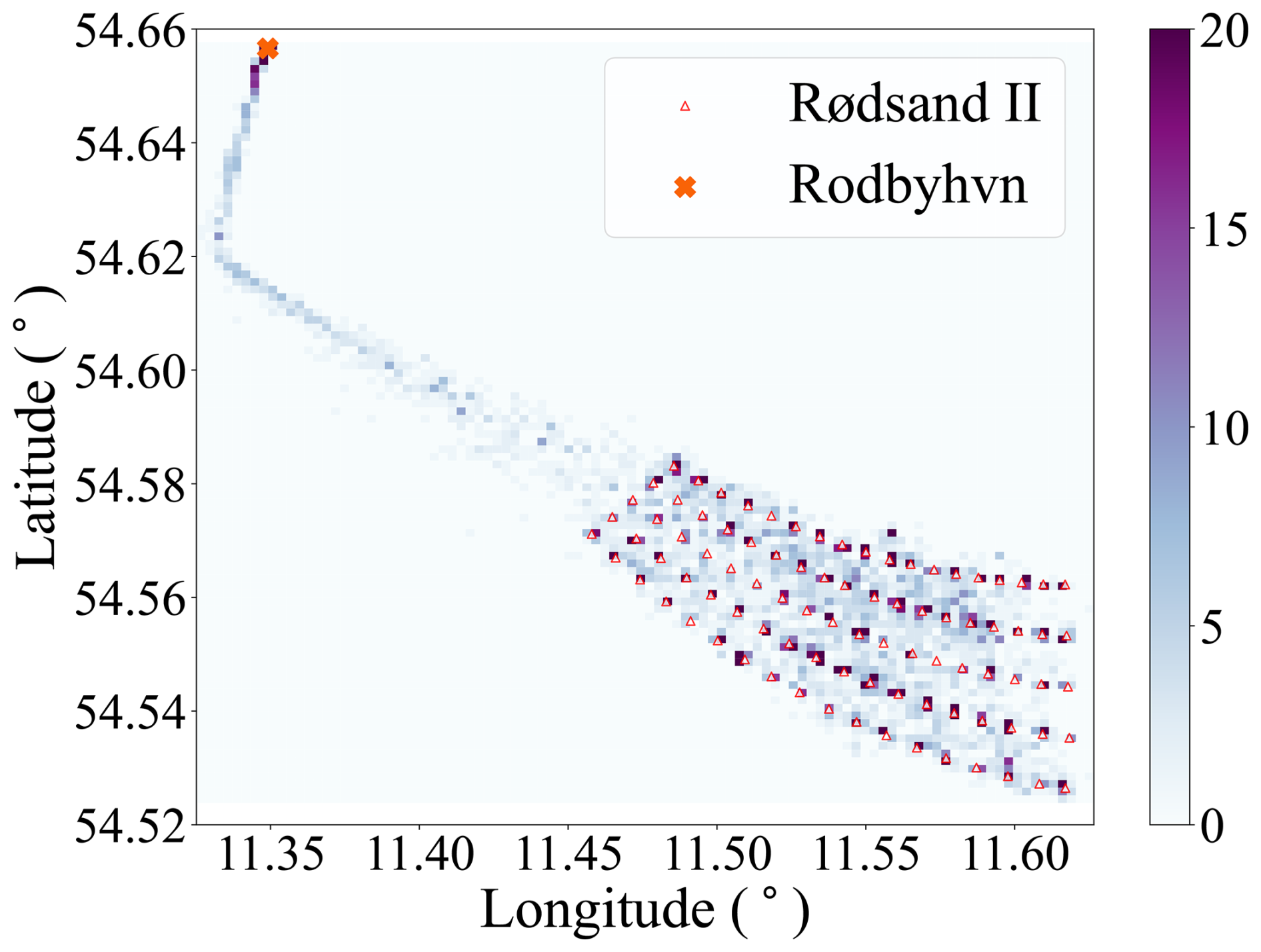
Figure 8 Spatial density map of the CTV’s position during the LOLLEX campaign. The colour scale indicates the cumulated time spent (in h) of recorded positions, with darker areas representing locations where the CTV spent more time. Red triangles mark the Rødsand II wind turbines. The cross marks the approximate location of Rødbyhavn harbour. The map is based on data recorded by the WindCubeV2 's internal IMU.

The CTV was located primarily in the harbour during the night and inside the wind farm during the day, as illustrated by Fig. 8. This figure uses a pseudocolour plot to visualise the number of hours the CTV spent at each location. The map reveals several high-density clusters, some exceeding 50 h, near individual wind turbines and the transformer platform. These high-density areas correspond to the turbines most frequently visited for operation and maintenance, as well as offshore idle time. Most turbines were visited at least once, ensuring that lidar measurements were collected across the entire wind farm during stationary periods. This widespread spatial coverage is a clear advantage of the vessel-based lidar setup. Such extensive spatial sampling would not have been achievable using wind lidars mounted only on buoys or fixed platforms.

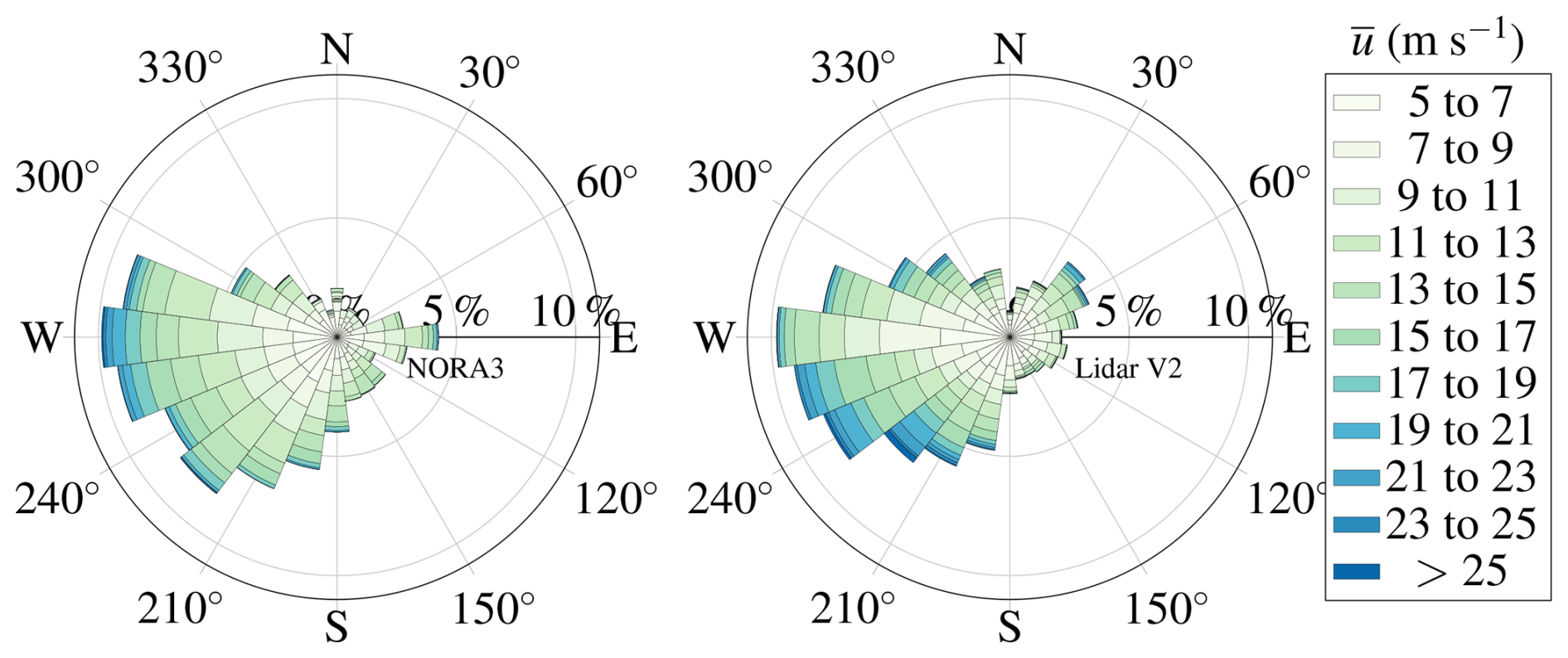
Figure 9 Wind rose for the mean wind speed at 150 m obtained with NORA3 (left) and WindCubeV2 (right) during the Lollex measurement campaign, from 9 October 2022 to 12 July 2023 (6624 h of data).

Figure 9 shows a comparison between the wind roses from NORA3 and WindCubeV2 data at 150 m above sea level. To improve clarity, only wind energy-relevant wind speeds (above 5 m s⁻¹) are included. The wind rose is based on 5623 h of data. Both NORA3 and the WindCubeV2 show that westerly winds dominate, with a median wind speed between 8 and 9 m s⁻¹ at 150 m altitude. The WindCubeV2 data indicate more frequent north-easterly winds and stronger winds from the sector between 210 and 260° than NORA3. Differences in wind direction between the NORA3 dataset and the WindCubeV2 measurements can be explained by two factors. First, the CTV carrying the lidar was not fixed in space and often remained near the harbour or inside the wind farm, while NORA3 data corresponds to a fixed offshore grid point. Second, the NORA3 model does not represent the effects of the Rødsand II and Nysted wind farms on the local wind field.

5 Results

This section compares the wind speed data from the two lidars mounted on the CTV with the NORA3 reanalysis before and after applying motion correction. The goal is to assess the overall performance of the motion correction method in addition to the evaluation of the consistency between the lidar data and NORA3. This comparison is important to build confidence for the case studies presented later in the paper. Further, four selected case studies are presented, each highlighting the potential and limitations of the chosen measurement setup. The first three case studies rely on the dual-lidars deployment on the CTV, focusing on a detailed characterisation of the marine atmospheric boundary layer and its potential interaction with a wind farm, while the fourth focuses on the lidar deployed on the transformer platform and its potential for wake detection and characterisation.

5.1 Motion correction results for mean wind speed profiles

Motion correction was applied to the full dataset, including WindCubeV2 measurements and WindCube100S DBS data. The corrected and uncorrected results are compared with NORA3 in Fig. 10. For the WindCubeV2, the correction increases the regression slope from 0.85 to 0.91 and bias value from 0.1 to 0.24 m s⁻¹, improves R² from 0.797 to 0.892, and reduces the RMSE from 1.9 to 1.5 m s⁻¹. For the WindCube100S, the correction increases the bias from −0.19 to 0.03 m s⁻¹, R² from 0.737 to 0.814, and slightly reduces the RMSE from 2.2 to 2.1 m s⁻¹, with the regression slope moving closer to unity.

For the WindCubeV2 lidars, the error metrics relative to NORA3 are similar to those reported in Cheynet et al. (2025), which were obtained using fixed lidar instruments. This suggests that the motion correction leads to performance comparable, in terms of these statistics, to that of fixed lidars. However, this does not imply that the motion correction is successful in all cases.

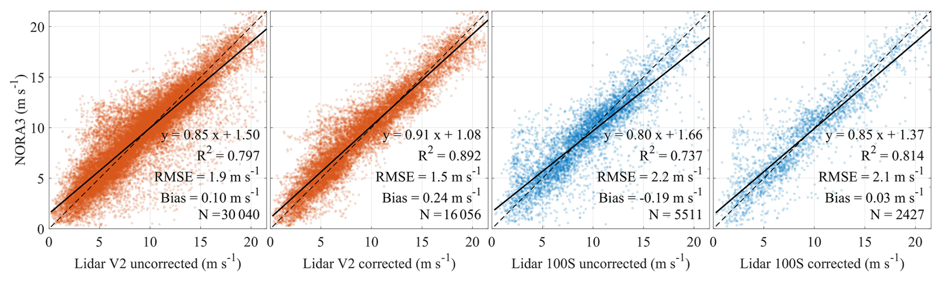
Figure 10 Scatter plots of 10 min mean wind speed from the WindCubeV2 (left two panels) and 5 min mean wind speed from the WindCube100S (right two panels) against NORA3 reference data for the entire campaign. Uncorrected data are shown in the first and third panels, and motion-corrected data in the second and fourth panels. The dashed line indicates the 1:1 relationship, and the solid black line the linear regression fit. Motion correction improves agreement with NORA3, reflected in regression slopes closer to unity, increased R², reduced RMSE, and reduced bias.

Figure 11 shows the ensemble-averaged bias and RMSE between NORA3 and the ship-based lidars' wind profiles during the campaign before and after motion correction. The WindCubeV2 and WindCube100S show a positive bias below 100 m, indicating that NORA3 overestimates wind speed at lower heights. The NORA3 hindcast does not consider wind-farm wakes, while the lidar measurements are affected by the flow deceleration caused by the farm, a phenomenon also documented at the FINO1 site (Podein et al., 2022; Cheynet et al., 2025). It is worth mentioning that NORA3 has a horizontal resolution of 3 km and represents boundary-layer flows more realistically than the earlier 10 km NORA10 hindcast (Haakenstad et al., 2021). Nevertheless, uncertainties in the representation of near-surface wind processes may remain. Evaluations of similar high-resolution wind atlas datasets (3 km) show that they reproduce near-surface wind characteristics fairly well, although certain aspects of boundary-layer dynamics, such as the structure of low-level jets, may still be imperfectly represented (Kalverla et al., 2020; Rubio et al., 2022).

As shown in Fig. 11a, the bias of the motion-corrected WindCubeV2 data becomes slightly more negative with increasing altitude. The variations in bias remain within ± 0.2 m s⁻¹ across the profile. For the WindCube100S, the bias is more positive below approximately 100 m, and its magnitude decreases, approaching −0.5 m s⁻¹ above 200 m after correction.

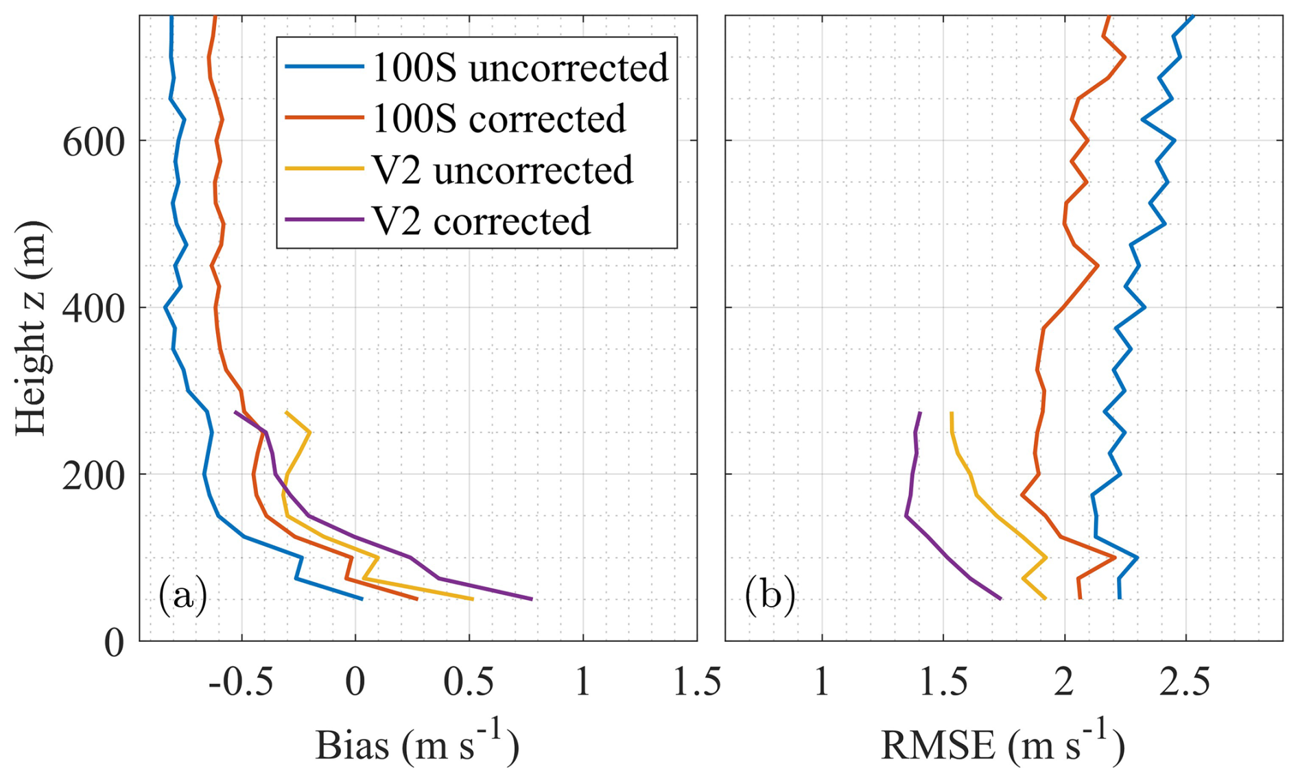
Figure 11 Ensemble-averaged bias (left) and root mean square error (RMSE; right) between NORA3 and ship-based DWL measurements at multiple heights during the LOLLEX campaign. Results are shown for the WindCube100S scanning lidar (uncorrected: blue; corrected: orange) and the WindCubeV2 wind profiler (uncorrected: yellow; corrected: purple), based on 10 min averages for the WindCubeV2 and 5 min averages for the WindCube100S.

The RMSE between the WindCubeV2 and NORA3 decreases with height for both uncorrected and motion-corrected data, with the corrected data showing systematically lower values (Fig. 11b). Above approximately 150 m, however, the RMSE increases again. In contrast, the RMSE between the WindCube100S and NORA3 increases slightly with height, with typical values around 2 m s⁻¹ after correction. The magnitude of the bias and RMSE is consistent with earlier validation studies of NORA3 in offshore and coastal regions (Cheynet et al., 2025). A local maximum near turbine tip height may reflect increased flow variability not captured by NORA3. The contrasting RMSE trends suggest that part of the height dependence reflects measurement characteristics rather than changes in model performance, with increasing uncertainty for the WindCube100S at higher altitudes. This interpretation is consistent with previous findings that NORA3 performance generally improves slightly with height above the surface (Cheynet et al., 2025).

5.2 Case study 1 – Kelvin-Helmholtz billows observations

This case study was presented in detail in Malekmohammadi et al. (2025), but the analysis was limited to the period between 12:35 and 13:00 UTC on 22 February 2023. Here, we expand upon that work to highlight the influence of CTV motion on velocity retrieval and to provide recommendations for the use of a scanning DWL on a moving vessel. For completeness, we summarise below the context in which Kelvin-Helmholtz billows (KHBs) were observed, but refer the reader to Malekmohammadi et al. (2025) for further details.

KHBs are wave-like structures caused by shear instability between air layers moving at different speeds (von Helmholtz, 1868; Stull, 1988). They typically form under hydrostatically stable conditions when vertical wind shear exceeds a critical threshold. This leads to dynamic instability and enhanced turbulent mixing, particularly vertical momentum transport. During the LOLLEX campaign, the scanning DWL on the CTV observed KHBs on several occasions. One of the clearest events occurred on 22 February 2023, between 12:30 and 13:00. The KHBs were captured in both the CNR and vertical velocity data, as shown in Fig. 12a and b. The time series reveals distinct KHB structures between 12:46 and 12:56 at altitudes ranging from 550 to 750 m. These structures evolved from small wave-like perturbations into billows that grew, overturned, and eventually dissipated. In the vertical velocity field, they appear as alternating zones of upward and downward motion.

Before the event, a bright and persistent CNR maximum is observed near 600 m (Fig. 12a). This maximum corresponds to aerosol accumulation beneath the capping inversion at the top of the stable boundary layer. Strong temperature inversions can suppress vertical turbulent mixing and limit dispersion, leading to the accumulation of aerosols below the inversion (Zhang et al., 2024). Vertical wind shear due to the change from typical sub-geostrophic wind speeds in the ABL towards geostrophic winds in the free atmosphere above can create favourable conditions for Kelvin-Helmholtz instabilities.

The KHBs were advected across the lidar beam over approximately 11 min, and their passage caused vertical mixing. This mixing is visualised by the broadening and dimming of the CNR maximum, which progressively descended downward to around 400 m by 13:00. However, a local maximum in the CNR remained visible until 13:30, suggesting that elevated aerosol concentrations persisted at around 400 m altitude, even after the dissipation of the KHBs.

Coincidentally, the lidar measurements, located approximately 37 m downstream of the turbine, captured the effect of the turbine on the local flow field. This appears in the vertical velocity time series as a band of enhanced positive vertical velocity between 100 and 200 m height, visible between 12:35 and 13:12 (Fig. 12b). The spatial extent of the enhanced vertical velocity band indicates a rotor-induced streamline deflection in the near-wake region. This interpretation is consistent with previous studies of near-wake dynamics (Whale et al., 2000; Hong et al., 2014; Dasari et al., 2019; Lanzilao and Meyers, 2024). SCADA data confirm that the turbine was operational during the observation period, with a nacelle orientation of approximately 167°, placing the lidar nearly directly downstream of the rotor.

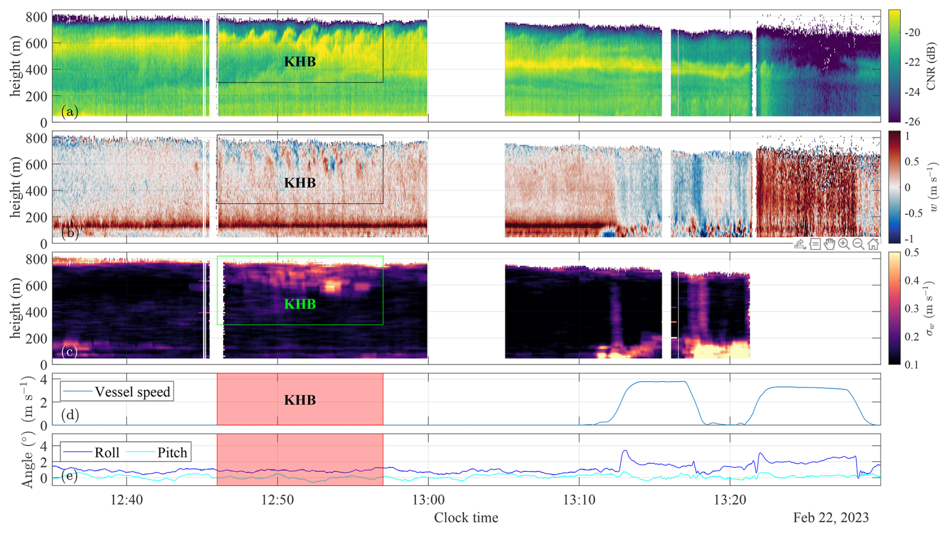
Figure 12 Time series of the Carrier-to-Noise ratio (CNR, a), instantaneous vertical velocity component w (b), and estimated moving standard deviation, σ_w(t), of the component w (c) obtained using the WindCube100S data in vertical stare mode from 12:35 to 13:30 on 22 February 2023. CTV absolute speed (d), roll and pitch angles (e) during the observational period.

The panel d and e of Fig. 12 show the vessel speed, roll, and pitch angles. Between 12:35 and 13:10, the CTV remained stationary with minimal roll and pitch. After 13:12, the vessel began moving away from the turbine, which led to a negative velocity bias in the WindCube100S data and the disappearance of the near-wake signature. The vessel speed increased to approximately 4 m s⁻¹ before becoming stationary again near 13:20, after which it resumed motion to a new location.

The observation of this KHB event revealed a significant increase in the variance of the vertical velocity component within a 400 m thick atmospheric slab, well above the region influenced by the turbine near-wake (Fig. 12c). In this case, no direct interaction between the KHBs and the wake was observed. However, such interactions may occur under different conditions, e.g. in a shallower ABL, within large wind farms where the internal boundary layer reaches the ABL top, or when KHBs form at lower altitudes, as briefly documented by Radünz et al. (2025). As highlighted by Malekmohammadi et al. (2025), the enhanced vertical mixing associated with KHBs, indicated by elevated vertical velocity variance, could accelerate wake recovery by entraining higher-momentum air downward. We therefore hypothesise that if KHBs overlap more directly with wind turbine wakes, they may enhance wake recovery under stable stratification. This hypothesis warrants further investigation.

Furthermore, when the CTV is in motion, the along-beam velocity data retrieved by the WindCube100S becomes significantly noisier, likely due to the combination of high translational speed and varying pitch and roll angles. This limits the instrument's ability to capture accurate velocity measurements and reduces the amount of usable data during periods of vessel motion. Consequently, operating the CTV in stationary mode is preferable when using scanning lidar for turbulence analysis, as it improves both the quality and availability of the retrieved data. Interestingly, the CNR data appear to be less affected by vessel motion. For instance, the dissipation of the KHBs into smaller wave-like patterns after 13:00 remains detectable beyond 13:10, even though the vessel was moving and the velocity data were considerably noisier. This highlights the utility of the CNR as a complementary data source, particularly under non-ideal motion conditions, for tracking coherent structures like KHBs.

5.3 Case study 2 – Downward turbulent flow

The second case study documents observation of a local increase of vertical turbulence on the same day (22 February 2023). This increase may have been promoted through buoyancy-driven downward turbulent motion from the top of the ABL reaching down to approximately 200 m above the surface. These measurements were collected before the vessel entered the wind farm under south-east wind conditions. The sunrise and sunset times in Rødbyhavn on 22 February 2023 were 06:21 and 16:36 UTC, respectively. Thus, the start of the scan coincided with the sunrise. The CTV was stationary at the beginning of the case study and started moving at 07:12 UTC. Figure 13 presents the instantaneous profiles of CNR (a), vertical velocity (b), and the moving standard deviation of w (σ_w) (c).

To determine the ABL top in this case, in addition to the CNR profiles, the profiles of wind speed and σ_w obtained from lidar measurements are illustrated in Figs. 14 and 15 a, respectively. The wind speed profiles show a local maximum between 0.9 and 1.0 km from 06:35 to 06:47 before decreasing significantly above 1 km, whereas the σ_w profiles, do not show a clear minimum. The ABL top is therefore inferred primarily from the CNR signal and is estimated to lie between 0.9 and 1.0 km.

Within this layer, the WindCubeV2 and WindCube100S DBS measurements reveal a local wind-speed maximum of 6 m s⁻¹ near 200 m, with NORA3 showing a similar maximum of about 5.5 m s⁻¹ around 150 m (Fig. 14). A strong negative wind-speed gradient occurs above this maximum. Consistent with this, the vertical wind velocity in Fig. 13b shows coherent regions of upward and downward motion emerging around 06:47 and persisting thereafter, indicating substantial vertical transport within the ABL. Prior to 06:47, the moving standard deviation of w (σ_w) is relatively uniform between 100 and 800 m, with weak turbulence (σ_w<0.2 m s⁻¹) (Fig. 13c). From 06:47 onwards, σ_w increases locally near 600 m and subsequently reaches values of approximately 0.5 m s⁻¹ between 400 and 600 m. The corresponding vertical profile of σ_w (Fig. 15a, between 06:47 and 07:00) also shows local increase of the vertical turbulent fluctuations at heights between 200 and 800 m above the surface.

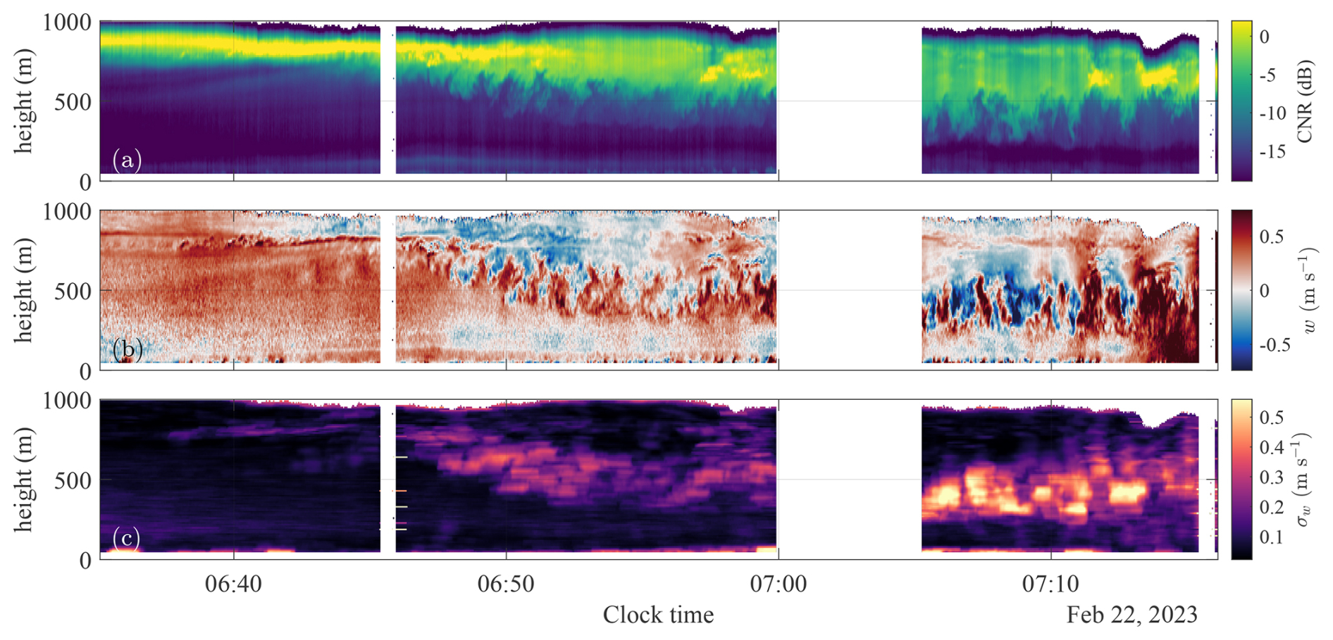
Figure 13 CNR (a), instantaneous vertical velocity component w (b), and estimated moving standard deviation, σ_w(t), of the component w (c) obtained using the WindCube100S on 22 February 2023 between 06:35 and 07:16 in the harbour.

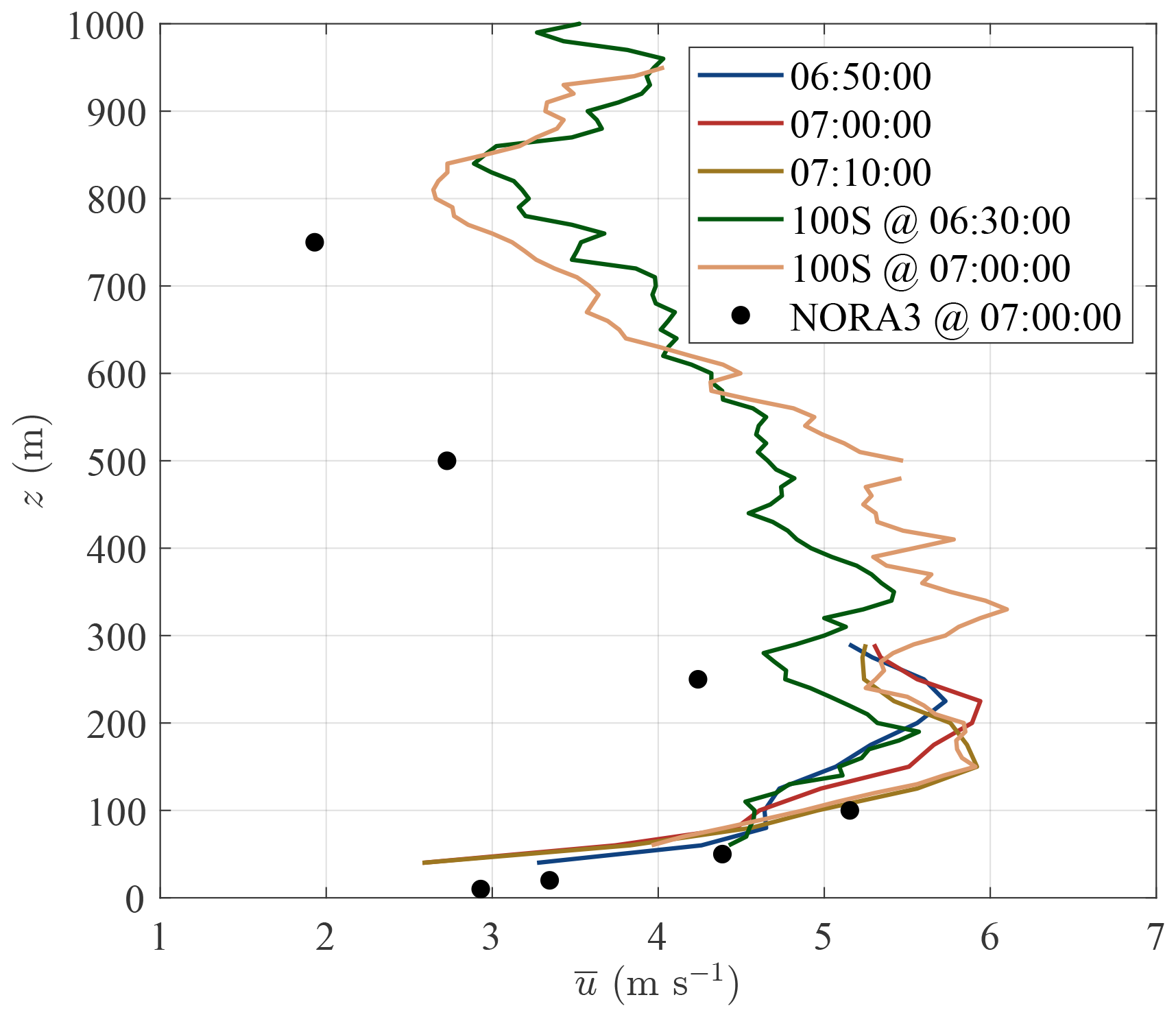
Figure 14 Profiles of the mean wind speed recorded by the WindCubeV2 and the WindCube100S on 22 February 2023 at multiple time windows between 06:30 and 07:10 in the harbour.

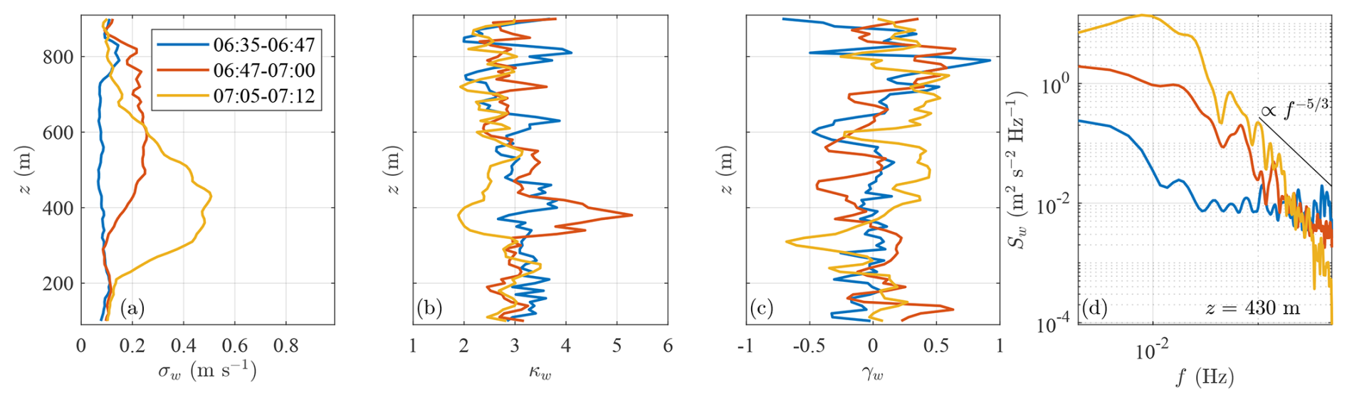
Figure 15 Profiles of the standard deviation σ_w (a), kurtosis κ_w (b), skewness γ_w of the vertical velocity component (c), and the power spectral density of S_w at 430 m (d). All panels are based on data recorded by the WindCube100S in the harbour on 22 February 2023 between 06:35 and 07:16.

Figure 15 also presents the vertical profiles of kurtosis (b), skewness (c) for three observational windows (06:35–06:47, 06:47–07:00, and 07:05–07:12), and the corresponding power spectral densities of w at 430 m (d). Prior to 06:47, the power spectral density S_w exhibits pronounced white noise at frequencies above 0.1 Hz, indicating that turbulence fluctuations are too weak to be reliably resolved by the WindCube100S scanning lidar. Between 06:47 and 07:00, the S_w spectra indicate improved detectability of turbulent fluctuations, although noise levels remain sufficiently high to partially obscure the effects of along-beam spatial averaging. After 07:05, vertical velocity fluctuations peak near 430 m, and the corresponding S_w spectrum shows reduced noise levels, with along-beam spatial averaging associated with the lidar probe-volume length becoming apparent at frequencies above 0.1 Hz, where the spectral slope steepens relative to the $-\mathrm{5}/\mathrm{3}$ inertial subrange. The pronounced spatial and temporal variability of σ_w reflects a non-stationary and vertically evolving boundary layer, suggesting the onset of downward transport from the boundary-layer top.

Although strong vertical shear is present and may contribute to shear-driven instability, this does not by itself demonstrate the presence of KHB. In our previous KHB observations (Malekmohammadi et al., 2025), the billows were characterised by a clear narrow-banded spectral peak, a well-organised periodic pattern in the time series, and a persistent kurtosis peak. In the present case, by contrast, the power spectral density of w shows a broader increase in energy across a range of frequencies rather than a narrow-banded peak, and the time series of w and CNR do not display similarly organised periodic structures. In this case study, the negative skewness peak around 300 m was used as an indicator consistent with turbulence generated by cloud-top radiative cooling; however, a negative skewness peak was also present in the KHB case of Malekmohammadi et al. (2025), indicating that this feature is not specific to one mechanism. In addition, local increases in kurtosis have previously been used as indicators of coherent KHB structures (Blumen et al., 2001; Malekmohammadi et al., 2025). In the present case, a local peak occurs between 06:45 and 07:00, which could suggest intermittent coherent structures consistent with KHB, but it disappears during 07:05–07:12, even though σ_w continues to increase. This behaviour contrasts with the persistent kurtosis peak observed during the KHB event reported in Malekmohammadi et al. (2025). Taken together, these features suggest that KHB cannot be excluded, but that the event does not exhibit the clear spectral and temporal signatures of a classical, well-organised KHB case; it is therefore interpreted more cautiously as intermittent mixing and entrainment near the ABL top.

Furthermore, radiative cooling at the top of stratocumulus clouds may be a plausible mechanism for triggering the observed buoyancy-driven turbulence (Wood, 2012). The resulting turbulence propagates downward, contributing to enhanced entrainment near the top of the cloud-topped boundary layer. This region is typically characterised by strong gradients in humidity and temperature that favour mixing processes. Following Hogan et al. (2009), turbulence influenced by cloud-top radiative cooling is often associated with negative skewness above the surface layer. In the present case, negative skewness of w, reaching values as low as −0.7 at 300 m (Fig. 15c), is observed between 07:05 and 07:12. This localised negative peak is absent before 06:47, prior to the increase in σ_w, while skewness becomes moderately negative (down to −0.4) between 400 and 700 m during 06:47–07:00. However, a negative skewness peak was also observed during the KHB event documented in Malekmohammadi et al. (2025), indicating that this feature is not unique to turbulence driven by radiative cooling. Although the present observations are qualitatively consistent with turbulence initiated near the ABL top, the absence of thermodynamic measurements near the boundary-layer top prevents a definitive attribution to radiative cooling. At the same time, the strong vertical shear suggests that shear-driven instabilities may also contribute, and the dominant mechanism therefore remains uncertain.

These observations demonstrate that turbulent mixing can develop under stable conditions and redistribute vertical momentum over several hundred meters, even without convective forcing or clear classical coherent structures such as KHBs. The non-stationary turbulence and its vertical extent suggest entrainment initiated near the ABL top and propagated downward through combined shear and buoyancy effects. Such vertically distributed entrainment may facilitate wake recovery in a wind farm by promoting the downward transport of higher-momentum air. These findings highlight the value of combining scanning and profiling DWLs on vessels to investigate entrainment processes.

5.4 Case study 3 – Internal wave observations

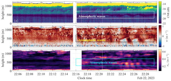
Case study 3 addresses observations of internal waves conducted in the harbour after the CTV returned from the offshore wind farm. The evening of 22 February was characterised by stable stratification, a wind speed of 10 m s⁻¹ at 100 m, a strong near-linear shear of approximately 0.06 m s⁻¹ m⁻¹ between 40 and 100 m (Fig. 16a) and a cloud cover above 600 m as indicated by the CNR profiles in Fig. 17a. As shown in Fig. 16a, the WindCube100S detected the presence of a low-level jet, with a maximum wind speed of 15 m s⁻¹ between 300 and 500 m above the surface. From 22:05 to 22:30, the lidar recorded wind conditions suggestive of internal atmospheric waves below the cloud-topped ABL. Such waves are often associated with the presence of low-level jets (Jia et al., 2019). In the present case, the observed wave-like motions may have been triggered by shear instability near the maximum of the low-level jet, where vertical wind shear was strongest.

Wave patterns begin to form at 22:16 and become visible in both the CNR, above 400 m, and the vertical velocity fluctuations from 200 to 600 m (Fig. 17a and b). These waves are not generated by wind farms and are therefore distinct from the so-called farm-generated gravity waves (Allaerts and Meyers, 2018). When internal atmospheric waves, including gravity waves, form upstream of a wind farm and at a height low enough to interact with the farm's internal boundary layer, they may enhance wake recovery by amplifying mixing and wake meandering (Feng et al., 2026).

Figure 17 shows the vertical structure of these oscillations, which span approximately 200 m in height. The wave-like motions are visible both in the instantaneous vertical velocity (panel b) and the corresponding standard deviation (panel c). The internal wave structure coincides with the nose of the low-level jet. A spectral analysis of the vertical velocity at 200, 400, and 600 m revealed a dominant periodic signal with a 2 min cycle during the wave event, as shown in Fig. 16b and c. The observed phase shift between altitudes suggests that vertical wind shear strongly influences the wave structure. No distinct spectral peak is observed prior to the occurrence of the waves (Fig. 16b), indicating the absence of wave activity during this earlier period. During the wave event (22:15–22:30), pronounced spectral peaks appear between approximately 200 and 600 m, consistent with the oscillations visible in the time series in Fig. 16c. After 22:30, clear spectral peaks remain visible between approximately 350 and 600 m, while no pronounced peak is observed at 200 m, suggesting that the wave packet initially reaches 200 m but later remains confined to higher altitudes near the nose of the low-level jet.

The spectral peak falls within the mesoscale range rather than the typical turbulence range, and is therefore more consistent with internal atmospheric waves than with turbulent eddies.

The observed period places these waves at the lower end of the internal gravity wave spectrum. For comparison, Banakh and Smalikho (2016) reported oscillation periods between 6.5 and 18 min in coastal terrain, while Jia et al. (2019) observed shear-driven gravity waves with periods exceeding 10 min. According to Sun et al. (2015), internal gravity wave periods typically range from 1 to 30 min, indicating that the 2 min period observed here is short but still within the expected range.

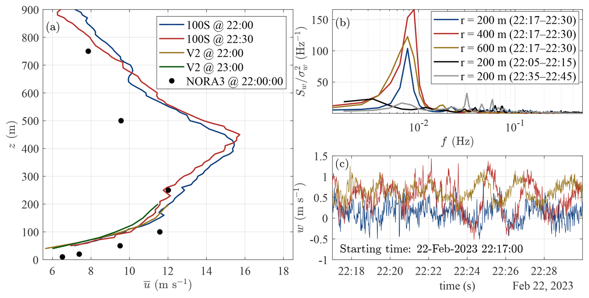
Figure 16 Profiles of the mean wind speed measured by the WindCubeV2 and the WindCube100S on 22 February 2023 between 22:00 and 22:35 in the harbour (a). Power spectral densities of the vertical velocity fluctuations from 200 to 600 m above the surface during the wave event (22:17–22:30) (b). The black (grey) solid line shows the power spectral density at 200 m prior (after) to the observation of the waves for comparison. Time series of vertical velocity corresponding to the PSD shown in panel (b) between 22:17 and 22:30 (c).

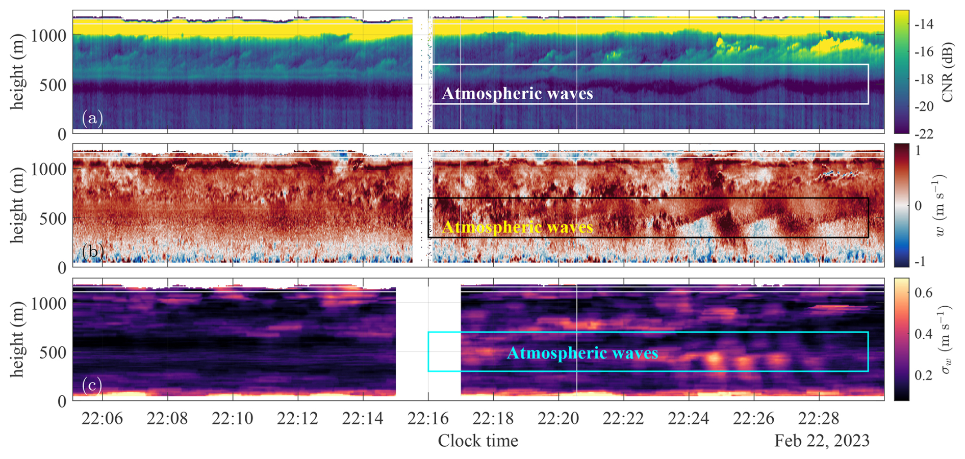
Figure 17 CNR (a), instantaneous vertical velocity component w (b), and estimated moving standard deviation, σ_w(t), of the component w (c) obtained using the WindCube100S on 22 February 2023 between 22:05 and 22:30 in the harbour.

As shown in Fig. 17c, the local increase in the standard deviation of vertical velocity extends to heights below 200 m, even though the CNR indicates that the wave-like pattern is strongest around 500 m. Given the proximity of the measurement site to the coast and its distance of about 20 km from the nearest offshore wind farm, it is possible that similar wave-like motions could occur above the wind farm itself. If so, such waves could enhance wake recovery by amplifying vertical momentum entrainment into the farm.

The previous case studies, along with this one, demonstrate the ability of scanning and profiling DWLs to capture dynamic processes in the ABL, including momentum entrainment associated with internal waves. However, limitations remain for a complete characterisation of internal atmospheric waves. In particular, the absence of co-located temperature and humidity measurements restricts our ability to study the stratification of the atmosphere in detail and, therefore, to identify the dominant wave generation mechanisms. While wind speed profiles confirm the presence of a low-level jet and support the interpretation of shear-induced wave activity, additional observations would be needed to distinguish between shear- and buoyancy-driven processes.

Moreover, although reanalysis products such as NORA3 could be used to estimate atmospheric stability (e.g., via the Bulk Richardson number), their temporal and spatial resolution is limited compared with the scales of the observed processes. A more robust assessment would require co-located, high-resolution profile measurements of temperature and humidity, e.g. by a passive microwave radiometer (Westwater et al., 2004; Rose et al., 2005), a Raman lidar (Lange et al., 2019; Wulfmeyer and Behrendt, 2021), or an infrared temperature profiler (Knuteson et al., 2004; Michaud-Belleau et al., 2025). To obtain such measurements, a HATPRO RG4 profiler was installed at Rødsand harbour at the beginning of the campaign. Unfortunately, the instrument was malfunctioning, and no usable data could be obtained.

5.5 Case study 4 – Wake observations

This case study presents preliminary results from RHI scans performed by the long-range scanning lidar installed on the transformer platform north of the Rødsand II wind farm. The limited joint data availability from the floating WindCubeV2 lidar and the platform-mounted lidar prevented a systematic analysis; however, a few representative cases can still be highlighted.

Case study 4 corresponds to an easterly mean flow observed by the platform-mounted lidar on 13 June 2023 between 12:11 and 12:25. At 100 m, the WindCube V2 lidar measured 9.2 m s⁻¹, about 3 m s⁻¹ lower than the NORA3 estimate of 12.1 m s⁻¹. This further indicates that the lidar measurements were affected by wind farm-induced velocity deficits, unlike NORA3, which does not account for the presence of the wind farm. At 100 m, NORA3 indicates a mean wind direction of 71°, compared with 69° measured by the WindCube V2 lidar.

In the PyWake simulations, the ambient vertical wind-speed profile is prescribed directly from NORA3, while the wind direction is taken as a single value obtained by interpolating the NORA3 wind-direction profile at hub height. Data from the WindCube 100S were not available during this period. At the time of the observations, the CTV was located on the southeastern side of the wind farm (Fig. 18), implying that the areas scanned by the platform-mounted lidar and the WindCubeV2 lidar were not collocated.

The NORA3 vertical wind-speed profile and the hub-height wind direction derived from NORA3 were used as input to the PyWake model (Pedersen et al., 2023) for wind-farm flow simulations. Since NORA3 does not account for the presence of the wind farm, it provides an estimate of the undisturbed upstream flow, whereas the WindCubeV2 lidar measurements are affected by turbine and wind-farm wakes. PyWake was therefore used to simulate wind-speed profiles at the location of the WindCubeV2 lidar using different wake deficit models. In addition, virtual RHI scans were generated to mimic the measurements from the scanning lidar on the transformer platform. These virtual scans reproduce vertical slices of the mean along-beam velocity component as observed by the lidar.

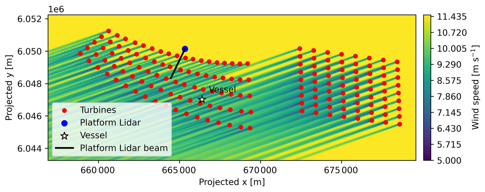
Figure 18 Horizontal cross-section of the mean wind speed at hub height for case study 4. In the PyWake simulations, the ambient vertical wind-speed profile is prescribed directly from NORA3 while the wind direction is taken as a single hub-height value of 70°. The TurboGaussian deficit model is used without blockage effects. The flow field is computed using PyWake with a downwind propagation scheme and a squared-sum superposition model, and is evaluated on a horizontal grid at hub height.

The comparison serves two main purposes. First, it provides a novel approach to assess the performance of wake deficit models implemented in analytical wake modelling frameworks. Second, it enables a qualitative evaluation of the lidar measurements, i.e. to verify whether the observed wake structures are consistent with simulations.

It should be noted that NORA3 does not necessarily provide a perfect estimate of the true upstream wind conditions. Discrepancies between model predictions and observations may therefore arise from several sources, including measurement noise, limitations of the wake models in representing real atmospheric conditions, or inaccuracies in the initial and boundary conditions derived from NORA3. For the purpose of comparing wake deficit models, these sources of uncertainty are of secondary importance, as all simulations rely on the same NORA3 input and are evaluated against the same reference measurements.

In PyWake, the PropagateDownwind wind farm model was adopted, in which wake effects are computed by propagating the influence of upstream turbines downstream and superimposing their wake deficits onto the undisturbed inflow. This formulation neglects upstream blockage effects, which were therefore not considered. A set of analytical wake deficit models was evaluated under identical inflow conditions, including NOJ (Jensen, 1983), TurboNOJ (Nygaard et al., 2020), BastankhahGaussian (Bastankhah and Porté-Agel, 2014), NiayifarGaussian (Niayifar and Porté-Agel, 2016), ZongGaussian (Zong and Porté-Agel, 2020), TurboGaussian (Ørsted, 2020), and GCL (Larsen, 2009). For Gaussian-based wake deficit models, a mirror ground model was used to account for sea-surface reflection. Wake superposition was treated using a squared-sum approach, and wake-added turbulence was modelled using the Crespo-Hernandez formulation (Crespo and Hernandez, 1996), assuming a uniform ambient turbulence intensity of 0.07, representative of typical offshore conditions (Cheynet et al., 2017a).

The inflow was prescribed using a UniformSite with a user-defined vertical wind-speed profile obtained by interpolating the NORA3 wind speeds as a function of height. The wind direction was prescribed as a single value obtained by interpolating the NORA3 wind-direction profile at hub height. Simulations were performed for the combined Rødsand II and Nysted wind farm layouts, implemented from measured turbine position data. All turbines were represented using a generic Siemens SWT-2.3-93 turbine (rotor diameter 93 m, hub height 69 m), with power and thrust coefficients prescribed from tabulated curves. No yaw misalignment, wind veer, or wake deflection effects were considered.

For each wake deficit model, the simulated flow field was sampled in two configurations. First, vertical profiles of the mean wind speed were extracted at the position of the floating WindCubeV2 lidar. Second, virtual RHI scans were generated by sampling the flow field in a vertical plane aligned with the scanning geometry of the platform-mounted lidar. The along-beam velocity was reconstructed by projecting the simulated horizontal wind vector onto the lidar line-of-sight, thereby neglecting any mean vertical velocity component. Differences between the present results and those reported by Souaiby and Porté-Agel (2024) may partly arise from differences in wake model selection, configuration, and the treatment of wake superposition and turbulence.

Figure 19 shows the vertical profile of the mean wind speed above the CTV during case study 4. The WindCubeV2 lidar profile exhibits negative wind shear below approximately 60 m and positive shear above, which is characteristic of waked flow. This is consistent with the horizontal flow field in Fig. 18, which places the vessel within a waked region.

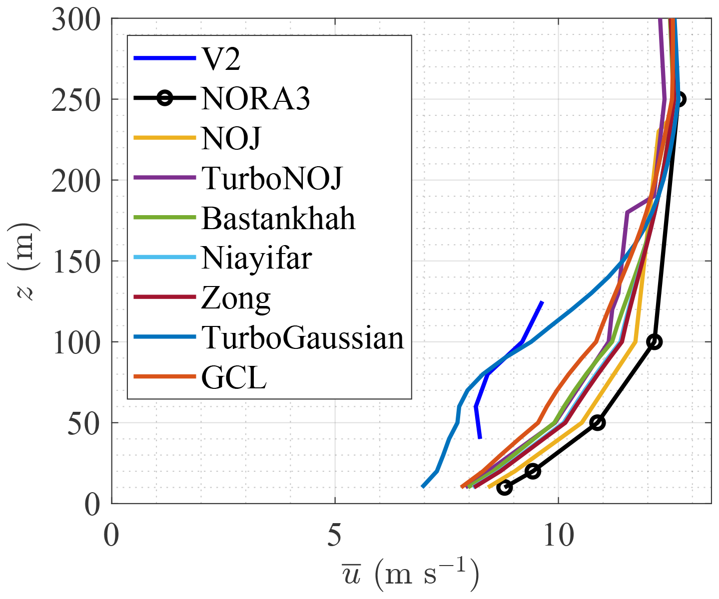
Figure 19 Vertical profiles of mean wind speed above the CTV during case study 4 under easterly flow conditions. In the PyWake simulations, the ambient vertical wind-speed profile is prescribed directly from NORA3, while the wind direction is taken as a single value obtained by interpolating the NORA3 wind-direction profile at hub height. The hub-height wind direction is 70^∘. The results are obtained from NORA3, the WindCubeV2 lidar, and PyWake simulations using different wake deficit models (NOJ, TurboNOJ, BastankhahGaussian, NiayifarGaussian, ZongGaussian, TurboGaussian, and GCL).

The PyWake simulations in Fig. 19 show that most wake deficit models underestimate the observed wake losses, resulting in higher wind speeds than measured by the V2 lidar. Only the TurboGaussian model provides close agreement with the observations. Although based on a single case, this result is consistent with Fischereit et al. (2022), who reported that commonly used analytical wake models underestimate wake deficits and overestimate wake recovery between the Rødsand II and Nysted wind farms, but did not include the TurboGaussian model. The TurboGaussian model, closely related to Ørsted's TurbOPark concept, produces stronger far-wake effects; in the present simulations, it yields longer wake extents and larger velocity deficits than the other Gaussian-based models, leading to improved agreement with the lidar observations.

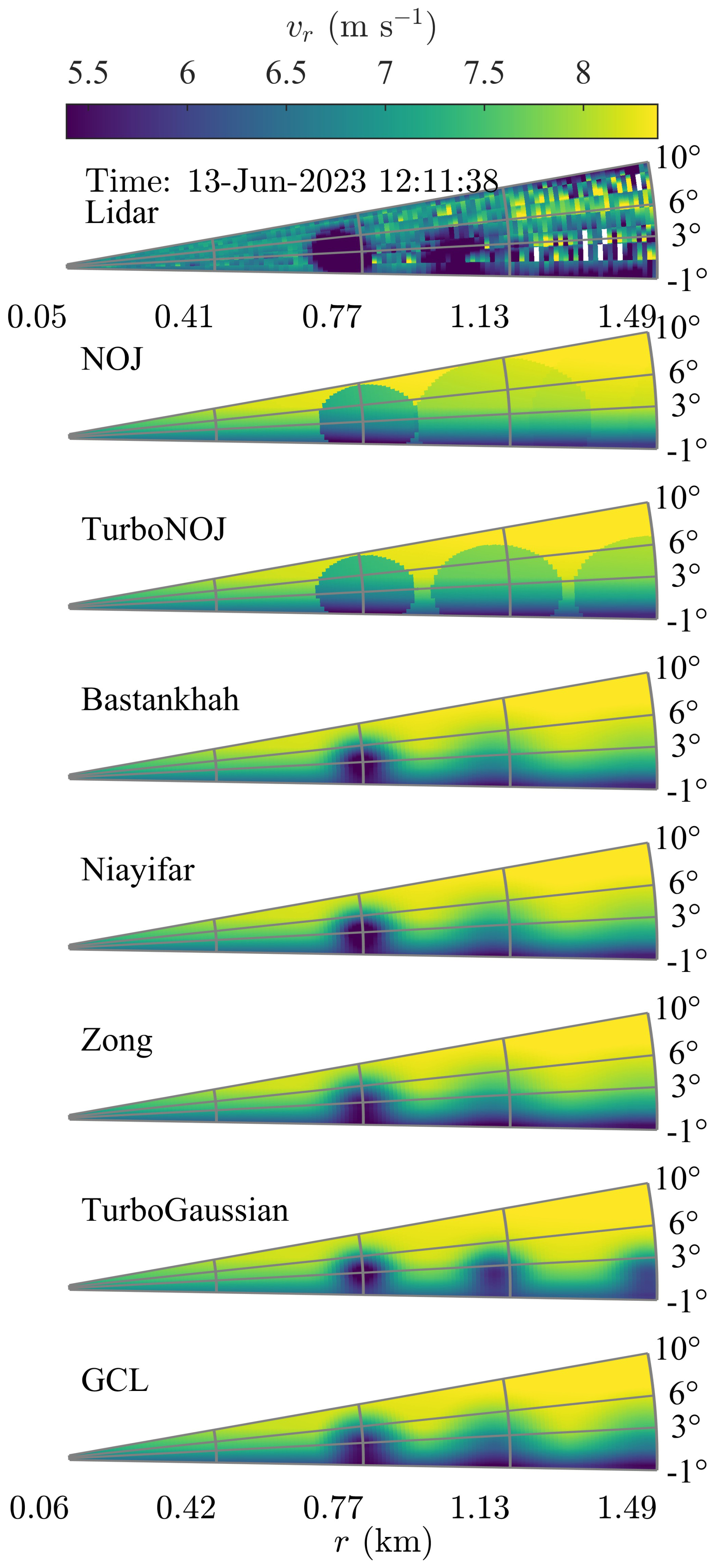
Figure 20 Comparison of the 14 min mean along-beam wind velocity from an RHI scan on 13 June 2023 at 12:11 (azimuth 206°). The top panel shows measurements from the platform-mounted lidar. The seven panels below show corresponding virtual RHI scans from PyWake simulations using different wake deficit models (NOJ, TurboNOJ, BastankhahGaussian, NiayifarGaussian, ZongGaussian, TurboGaussian, and GCL). In the PyWake simulations, the ambient vertical wind-speed profile is prescribed directly from NORA3 while the wind direction is taken as a single hub-height value of 70°.

Figure 20 compares the 14 min mean along-beam wind velocity measured by the platform-mounted scanning lidar during an RHI scan on 13 June 2023 at 12:11 with corresponding virtual RHI scans obtained from PyWake simulations. The comparison is performed using an averaged flow field, consistent with the steady-state assumption of the PyWake simulations. Both measurements and simulations reveal multiple turbine wakes.

Both measurements and simulations capture wakes from individual turbines within the Rødsand II wind farm. The simulations primarily resolve three distinct wakes, while Fig. 18 suggests that the flow may also be influenced by additional far-wake contributions from the upstream Nysted wind farm. Such farm-to-farm interactions are known to enhance wake losses at Rødsand II (Hansen et al., 2015; van der Laan et al., 2015); however, this contribution cannot be unambiguously isolated in the RHI scans of the platform-mounted lidar. In Fig. 20, the wake of the nearest turbine, located approximately 0.7 km from the lidar, is clearly identified in both measurements and simulations. The alignment of subsequent wakes, around 1.0 km downstream, is slightly less consistent between simulations and observations. In particular, a third wake is predicted by the simulations but is not clearly visible in the measurements, likely due to measurement noise.

Discrepancies between simulated and observed wake structures can arise from several factors. Small variations in wind direction can significantly shift wake positions in virtual RHI scans when NORA3 is used to prescribe the inflow. Additional sources of mismatch include wind veering (Bodini et al., 2017), yaw misalignment due to turbine control, and large-scale effects such as the Coriolis-induced deflection of the Nysted farm wake (van der Laan et al., 2015). Differences in wind speed between simulations and measurements are further influenced by uncertainties in the upstream inflow. During the campaign, upstream conditions were not systematically measured, as vessel-mounted lidars were often located in sheltered harbour environments or within the wind farm. Although NORA3 provides a practical inflow estimate, it may be less reliable under moderate and weak wind conditions. In periods of strong winds, when the vessel could not operate within the farm, wake validation relied solely on platform-based lidar observations.

Overall, several thousand RHI scans were collected during the campaign, providing a unique dataset for the validation of analytical wake models at Rødsand II. While the present qualitative comparison suggests that the TurboGaussian (TurbOPark-type) model performs well for this case, further work is required to better characterise inflow conditions, for example using SCADA data, and to extend the analysis to multiple cases. Future work should include systematic quantitative error metrics, such as root-mean-square error or bias, applied to both RHI scans and vertical wind speed profiles to identify the most suitable wake deficit models.

6 Discussion

CTV-based wind lidar measurements overcome several key limitations of DWLs mounted on fixed platforms or buoys, while also introducing their own set of constraints. In this study, observations within the offshore wind farm were largely restricted to daytime working hours (typically 07:00 to 19:00), limiting the ability to capture nighttime conditions. Although measurements were continuously recorded, including during nighttime in the harbour, no observations within the wind farm were obtained outside daytime operations.

In addition, safety regulations prohibit CTV operations when significant wave heights exceed 2 m or wind speeds surpass 12 m s⁻¹, reducing data availability during strong-wind or swell events. In contrast, buoy-based lidars can operate continuously, including during high-wind conditions, though they lack the flexibility to capture different spatial locations. However, under severe wind and wave conditions, buoy motion can become too large for reliable wind measurements, leading to a significant degradation in data quality. In such cases, fixed platforms provide the most suitable approach for studying the atmosphere under strong wind and wave conditions.

The WindCubeV2 maintained considerably higher data availability during the campaign compared to the WindCube100S (by a factor of about 3.5). The WindCube100S showed a higher rate of scan interruptions, which we attribute not only to its mechanical configuration, specifically the relatively heavy two-axis external scanner head used to adjust both azimuth and elevation angles, but also to its sensitivity to platform motion. In particular, translational motions of the vessel appear to contribute to data loss and incomplete scans. In contrast, the WindCubeV2 uses optical switching without moving parts for beam steering (Peña et al., 2013; Newman et al., 2016), making it more robust under dynamic conditions. For the vertical staring mode conducted between 25 January and 28 August 2023 (approximately 9900 scans), 65 % of the WindCube100S scans were flagged as incomplete (scan duration <10 min) and excluded, while only 30 % reached the full 25 min duration.

Moreover, power supply considerations are an important factor when installing lidars on offshore vessels. Each vessel has a different electrical configuration, which influences how equipment can be safely integrated. In this campaign, the CTV required a daily power reset, which posed a risk to the WindCube100S due to its higher power demands and limited internal buffering. To address this, the lidar was connected to an external uninterruptible power supply (UPS) housed in a watertight enclosure. This configuration ensured stable operation during brief power interruptions. Future deployments can benefit from standardised power interface protocols and pre-tested UPS systems to improve installation efficiency and system robustness across different vessel types.

In principle, a dual-lidar setup like the one tested here could also be installed on a buoy. However, this would require careful consideration of platform stability and instrument design. Scanning DWLs are physically larger and more mechanically complex than lidar wind profilers, and most commercial models do not include active motion correction. Operation on a floating platform would therefore necessitate additional stabilisation measures or dedicated post-processing procedures. While motion correction is routinely applied to lidar wind profilers on buoys, extending this capability to scanning lidars requires further development. Alternatively, vessels such as CTVs provide a more stable and spacious platform. Among available offshore platforms, the CTV offers a cost-effective and mobile solution for short-term campaigns in shallow coastal areas.

Finally, the success of this campaign was supported by favourable environmental conditions. The measurement site was located in a shallow-water region with low average wave heights. The surrounding coastal topography and the short distance to the harbour enabled nearly daily access to the wind farm. These factors made it feasible to implement a mobile lidar strategy using a CTV. In deeper waters or more remote offshore locations, this approach would require significant adjustments. Vessels may not be able to visit the site daily, resulting in fewer data collection opportunities. Harsher sea states would increase platform motion, leading to greater uncertainty in the retrieved wind velocities due to tilt and translation effects. The exposure to rough conditions may also increase the risk of contamination or damage to the lidar optics, for example, due to sea spray on the scanner head.

To address these challenges, future campaigns may consider integrating real-time motion correction systems. One promising approach could involve gyroscopic self-stabilising platforms as shown in Achtert et al. (2015). Such systems could minimise the impact of platform tilt and reduce the reliance on post-processing corrections. While these systems may not be practical for small buoys due to size and power limitations, they could be feasible on larger vessels or semi-permanent floating platforms. Further investigation into active stabilisation methods for scanning lidars could help extend mobile measurement strategies to more demanding offshore environments.

7 Conclusions

The study presents new measurement of mean wind speed and vertical turbulence above an offshore wind farm as well as observations of wind turbine wakes, collected during the LOLland offshore Lidar EXperiment (LOLLEX), resulting in a unique dataset for wind energy and boundary-layer research.

The campaign introduced a novel dual-lidar setup on a crew transfer vessel (CTV), combining a scanning DWL and a Doppler lidar wind profiler. This mobile platform enabled flexible sampling of the atmospheric boundary layer (ABL) at various positions and under different wind conditions. To complement these mobile observations, a long-range scanning lidar was installed on a transformer platform at the northern edge of the Rødsand II wind farm. This fixed lidar provided continuous, high-resolution range-height indicator (RHI) scans along a fixed line of sight across the wind farm. The CTV-mounted scanning lidar enabled the study of entrainment processes up to about 2 km above the surface, while the platform-mounted scanning lidar provided detailed observations of wake structures within the lower 300–400 m of the atmosphere. The campaign lasted one year and produced several thousand hours of Doppler lidar data.

This study presents the potential of the measurement setup using four case studies. These examples highlight different entrainment-related processes and demonstrate the complementarity of DWLs deployed on mobile and fixed platforms:

1. Kelvin-Helmholtz billows (KHBs) were captured at altitudes between 550 and 750 m, indicating increased vertical mixing under stable conditions. This case illustrates how the vertical stare mode can be used to quantify turbulence statistics associated with shear instabilities (Malekmohammadi et al., 2025), but also reveals how vessel motion can significantly degrade the quality of scanning lidar data.

2. A case of downward turbulent mixing was observed during one morning, where momentum was transferred from the top of the ABL to lower levels, with no clear signatures of classical structures such as KHBs. This transient phenomenon, which may involve cloud-top cooling, shows that vertical entrainment can occur deeper into the boundary layer than documented in the first case study.

3. Internal atmospheric waves with a 2 min period were detected near the nose of a low-level jet. These shear-induced oscillations suggest that vertical momentum entrainment was likely driven by both strong height-dependant wind shear and wave-driven mixing.

4. Wake profiles inside the wind farm were recorded using RHI scans from the platform-mounted lidar. These were compared with PyWake simulations, providing valuable data for wake model validation. For this case, the TurboGaussian wake deficit model showed the best agreement with the observations. This case demonstrates that the campaign was not limited to turbulence studies but also supports direct observations of wake deficits, which are an essential component of understanding wake recovery.

Together, these results show that scanning lidars and lidar wind profilers can detect dynamic ABL processes relevant to vertical momentum entrainment. They also demonstrate the value of mobile lidar systems for offshore measurements, especially when flexibility in spatial coverage is needed.

Still, several limitations remain. The scanning lidar was highly sensitive to vessel motion, and data quality degraded significantly while the CTV was in transit. Motion correction was only applied in post-processing to the lidar wind profiler. The use of a CTV also restricts operations to relatively calm sea states (significant wave height H_s<2 m) and moderate wind speeds ($\stackrel{\mathrm{‾}}{u}<\mathrm{12}$ m s⁻¹), limiting data availability outside the harbour. In addition, the lack of co-located temperature and humidity measurements prevented a full characterisation of atmospheric stratification, making it difficult to separate buoyancy- and shear-driven processes.

The dataset collected during the LOLLEX campaign represents, nevertheless, a valuable resource for wind energy science and boundary layer meteorology. Future studies using this dataset could explore the following:

1. A more detailed evaluation of near-wake measurements. Case study 1 showed that vessel-mounted lidars can detect near-wake structures. The LOLLEX campaign provides a unique opportunity to investigate this further, as it includes numerous high-resolution scans collected at varying distances and angles relative to turbine wakes.

2. Combining data from the fixed platform lidar and the vessel-mounted lidars. This could give a more complete picture to understand wind turbine wake recovery by using wind velocity data across the rotor plane, both in the horizontal and vertical directions.

3. Using vertical stare scans from the scanning lidar to estimate the atmospheric surface layer depth. This approach can follow methods such as those proposed by Puccioni et al. (2024). Accurate estimation of ABL depth is important for modelling wake recovery and vertical momentum entrainment in offshore wind farms. Comparing these lidar-based estimates with boundary layer depths from reanalysis datasets would help assess the reliability of reanalysis products in coastal regions of Northern Europe.

4. Adding instruments such as microwave radiometers, radiosondes, or ultrasonic anemometers could help describe the vertical temperature structure and near-surface turbulence more accurately.