EigenFlux: a stable multi-stream radiative transfer method for strongly scattering media

Radiative transfer in strongly scattering media remains computationally challenging, particularly for systems with highly asymmetric phase functions and large optical depths, where conventional discrete-ordinate approaches may suffer from numerical instability, slow convergence, or loss of accuracy. We present EigenFlux, a multistream radiative transfer framework based on eigenmode decomposition, natural-reflectance stabilization, and flexible mesh-based angular discretization. Unlike previous approaches relying primarily on global polynomial expansions, EigenFlux permits localized resolution of phase functions with strongly forward scattering or significant backward-scattering components while preserving flux conservation and numerical stability. The method is evaluated across 957 test cases spanning asymmetry factors from $g=-\mathrm{0.998867}$ to g=0.998867 and single-scattering albedos from ω=0.0014660 to ω=0.9999995, including extreme multiple-scattering regimes that are difficult for conventional solvers. Comparisons with DISORT show 748 times better accuracy and 10 times faster execution for number of streams greater or equal to 168. EigenFlux maintained stable solutions for asymmetry factors exceeding $\mid g\mid >\mathrm{0.99}$, although stability is weaker for absorption levels less than 0.10. Analysis of the eigenspectrum reveals the emergence of asymptotic diffuse transport regimes in optically thick systems (thick/deep enough for the reflectance to reach its natural limit) and persistent direct-beam structure in semi-transparent media. These results suggest that EigenFlux provides a stable and flexible framework for radiative transfer calculations for atmospheres, snow and ice, ocean optics, pigments and coatings, remote sensing, and graphics rendering, particularly in cases involving extreme scattering asymmetry.

1 Introduction

The fundamental theory of light scattering in the atmosphere was developed by Lord Rayleigh in 1871 (Rayleigh, 1871). Rayleigh scattering remains fundamental to the field of radiative transfer today. The earliest known formulations of the modern radiative transfer equation (RTE) were published by Eugen Von Lommel in 1887 (Lommel, 1887), and an integral version by Orest Chwolson in 1889 (Chwolson, 1889). However, neither publication spread to the general academic community (Mishchenko, 2013).

Schuster (1905) used hemispheric isotopy to develop and publish a two-stream RTE and its analytical solution and has been traditionally credited with originating the RTE, although a similar two-stream approximation was presented in Eddington (1916). Papers by Schwarzschild (1906, 1914), and by Milne (1921) on thermodynamic equilibrium within solar and stellar atmospheres led to the establishment of the RTE in its general form. A full analytic theory of the RTE was developed and published in Chandrasekhar (1950).

In the meantime, Kubelka and Munk (1931); Kubelka (1948) developed a simplified two-constant RTE and its solution that is equivalent mathematically to Schuster's. Whereas Eddington and Shuster's two-stream RTE and subsequent modifications (Petty, 2006; Liou, 2002) have been considered only appropriate for mediums without strong asymmetry, Kubelka-Munk's method is effective for determining the reflectance of materials with strong scattering. As a result, K-M and its modifications have become the standard for use by the painting and coating industries (Koleske, 1995) where the most useful pigments tend to be those with extreme scattering properties. A modern study which uses the K-M method is the Lawrence Berkeley National Laboratory's study into pigments for roofing materials that show color in the visible spectrum, but are transparent in IR and UV so as to remain cool even under solar heating (Akbari et al., 2004). The study determined the scattering and absorbing properties of 85 candidate materials. Most materials were found to be strongly forward scattering (Levinson et al., 2005).

Researchers in atmospheric physics/chemistry and oceanographers were interested in solutions to the full RTE in order to understand the effects of solar flux. The 1970's saw the development of a variety of RTE solvers based on Chandrasekhar (1950), including the popular DISORT solver (Stamnes et al., 1988) available as public source code, both as a stand-alone distribution (LLLab, 2023) and as part of the RadTranLib distribution (Emde et al., 2016). Astronomers and metereologists were interested in the RTE as a way of understanding the albedo of the Earth and other planets (Coakley, 2003). The Bi-Directional Radiation Field (BDRF) was formulated and standardized as part of this understanding (Nicodemus et al., 1977; Torrance and Sparrow, 1967). Snow and ice are particularly important materials in determining the albedo of the Earth, and microwave sensing has become an important tool for characterizing current snow and ice levels. Current algorithms such as the Discrete Ordinates method are being supplied as part of RTE solvers with custom models for the highly forward scattering and low absorption features of snow and ice (Hamre et al., 2004; Ehn et al., 2008; Picard et al., 2018).

Application of the RTE to oceans began as early as 1922 when Raman (1922) invoked scattering as part of explaining the color of the sea. Scattering due to suspended particles (turbidity) and water turbulence play a major role in determining the color (Shoulejkin, 1923). The resulting mathematics was given a firm footing by Preisendorfer's 6 Volume Hydrologic Optics (Preisendorfer, 1968, 1976; Mobley, 1994). Akkaynak and Treibitz (2019) provides an interesting example of the use of the RTE in color-correction of underwater imaging. The Hydrolight tool (Mobley, 2020) is a commercial tool that can directly solve hydrological depth-varying absorbance and scattering problems, including systems with strong forward scattering. It is coded specifically for hydrological problems and does not address atmospheric radiative transfer or radiative transfer within pigmented materials.

A simplified form of the RTE was introduced by Blinn (1982) as an approach to rendering realistic scenes in computer graphics in 1984. This was expanded into a generalized Light Transport Theory a few years later by Kajiya and Von Herzen (1984). This initial work focused on models that were computationally light and resulted in realistic appearances, but were not necessarily physically accurate. Advances in computer technology have allowed the increased use of physically-realistic models (Pharr et al., 2023). The complexity of rendering lighting and atmospheric effects in computer-generated imagery means that the leading rendering technology is based on ray-tracing and Monte-Carlo sampling. These methods provide an important alternative to the more traditional RTE solvers. An example is the MYSTIC code (Emde et al., 2010) which is included in the RadTranLib public source distribution (Emde et al., 2016) along with the more traditional DISORT solver (Stamnes et al., 1988).

In addition to the pigments mentioned above, many key components of meteorological concern show strong forward scattering as well. Stamnes et al. (2011) reports $g=\mathrm{0.85},\mathrm{0.89},\mathrm{0.997}$ for air bubbles, snow grains, and brine pockets respectively. Clouds are strongly forward scattering and have strong backward scattering components (Garcia and Siewert, 1985) (see Fig. 11 below). Materials with true negative asymmetry are less common, but $g<-\mathrm{0.4}$ have appeared in theoretical studies of engineered materials (Varytis and Busch, 2020).

The Mesh Approximates (MA) method presented here is closely related to the classic Discrete Ordinates (DO) method presented by Chandrasekhar (1950) (we follow the presentation of Goody and Yung, 1989 and the paper by Stamnes et al., 1988). Both methods start with the integro-differential equation Eq. (3) with boundary conditions for the diffuse intensity with an explicit expression for the direct intensity. The DO method first defines a finite-dimensional approximation of the integral terms to generate a linear ODE. That finite-approximation uses a Legendre approximation of the phase matrix, and Gaussian quadrature for the integrals, which is mathematically equivalent to using Legendre polynomial expansions for the integrands. To solve the resulting Ordinary Differential Equations (ODE), DO performs an eigenvalue decomposition to get a system of uncoupled ODEs, half of which are unstable. DO expresses the uncoupled ODEs and boundary conditions as an algebraic eigenvalue problem, which is then solved using specialized algorithms for that purpose.

The MA method first approximates the original equation using a piecewise-linear approximation of the phase matrix and the diffuse intensity, with exact evaluation of the resulting integrands over each piece-wise linear interval. As in the previous method, the next step is to use an eigenvalue decomposition to solve the resulting Ordinary Differential Equations (ODE) to get a system of uncoupled ODEs, half of which are unstable. It stabilizes the uncoupled ODEs by initializing their solution with a natural reflectance assumption (equivalent to the assumption of an semi-infinite atmosphere). Piecewise-linear mesh approximations are again applied along the depth axis and to the boundary conditions in order to generate a well-conditioned linear system which can be solved with standard algorithms. The natural reflectance solution can then be used to generate the general two-boundary solution through a linear combination of the downward natural reflectance solution starting at the top boundary, and with an upward natural reflectance solution starting at the bottom boundary. The linear combination is chosen to satisfy the original boundary conditions at the two boundaries.

The DO method is limited in the fit that can be obtained using Legendre polynomials, which require high orders of approximation to avoid oscillations at the end-points, making it difficult to use for approximating those scattering phase functions which are strongly forward or have a significant backward scattering component. The MA approach allows for the use of any subdivision of the ordinates, both for the multi-streams and along the depth axis. This allows for the use of meshes designed to resolve the underlying dynamics, for forward scattering problems with more than 0.99 asymmetry for the existing implementations.

Like the DO, the base MA algorithm is limited to application to homogeneous media. Inhomogeneous media are managed by introducing multiple homogeneous layers with varying characteristics which can be combined into an overall heterogeneous solution. In its existing implementation, MA is limited to plane-parallel geometry, although the use of pseudo-spherical geometry is contemplated for the future.

Based on these considerations, there remains a need for a radiative transfer method that is numerically stable, computationally efficient, and accurate for both optically thick and semi-transparent systems, including systems with highly asymmetric scattering phase functions while also promoting transparency and reproducibility through open implementation. In this paper we introduce EigenFlux, a multistream radiative transfer model based on Mesh Approximation with an eigenmode formulation combined with flexible angular discretization and localized basis functions. The method is designed to preserve stability and conserve flux, while accurately describing strongly forward-scattering systems. We evaluate the approach across a broad range of asymmetry factors and single-scattering albedos, including extreme scattering regimes that are challenging for conventional discrete-ordinate methods. Finally, we compare the behavior of EigenFlux with established approaches and discuss potential applications in atmospheric science, ocean optics, remote sensing, material science, and graphics rendering.

2 Methods

2.1 Radiative Transfer

We investigate radiative transfer though a homogeneous media, illuminated at its top boundary and a reflective/absorptive surface at its bottom boundary, that contains a uniform mix of particles which may absorb or scatter light particles that are traveling through the media. We will limit this investigation to the plane-parallel situation, in which we only model the depth to which a light particle has penetrated, (increasing as the light particle descends deeper), the relative velocity (the cosine of the angle of travel relative to the vertical), and its azimuth (the angle of travel relative to the medium's “north”). The intensity function is interpreted here as the probability that a light particle is at depth y in the media, and has a relative velocity of v, where v=cos (θ). So (v=1, $\mathit{\theta }=\mathit{\pi }/\mathrm{2}$) is straight down, (v=0, θ=0) is horizontal, and ($v=-\mathrm{1}$, $\mathit{\theta }=-\mathit{\pi }/\mathrm{2}$) is straight up.

The particles may either absorb or scatter a light particle encountering them. The process of a light particle travelling until it is absorbed or scattered out of the beam is known as extinction, and the expected path length of the process is the extinction path length. Upon extinction, the fraction of the particles that are then scattered is the single scatter albedo also known as the scatter fraction. EigenFlux currently does not consider thermal emission or inelastic scattering from the particles. The scatter distribution is determined by a rotationally symmetric phase function k(v) with asymmetry g measuring the expected amount of back scatter vs. forward scatter, $g=\int \mathrm{2}\mathit{\pi }vk\left(v\right)\mathrm{d}v$ where g=1 is full forward scatter and $g=-\mathrm{1}$ is full backward scatter. The scattering matrix is given by

$$K(v,w;a-b)=k\left(vw+\cos (a-b)\sqrt{\mathrm{1}-v^{\mathrm{2}}}\sqrt{\mathrm{1}-w^{\mathrm{2}}}\right)$$

Further information and background can be found in the references Goody and Yung (1989); Koleske (1995); Petty (2006).

2.1.1 Key Variables and Functions

• θ= Angle of travel of light particle, relative to vertical

• ϕ= Azimuth of travel of light particle, relative to north

• $v=\cos \mathit{\theta }=$ Velocity relative to vertical

• $(v,a)=$ Polar cosine and azimuth angle of incident vector

• $(w,b)=$ Polar cosine and azimuth angle of scattered vector

• x= Depth

• y= Depth scaled to extinction path length

• z= Exponential depth $z=e^{-y/{\widehat{y}}_{\mathrm{05}}}$

• $\stackrel{\mathrm{̃}}{I}(v,x,\mathit{\varphi })=$ Intensity distribution

• $I(v,y,\mathit{\varphi })=$ Intensity distribution with respect to y

• $s(v,\mathit{\varphi })=I(v,\mathrm{0},\mathit{\varphi })=$ Intensity distribution at top boundary (source illumination)

• $K(v,w,a-b)=$ Normalized phase scattering distribution (parametrized by g)

2.1.2 Model Parameters

• σ= Extinction path length for light to interact with particles

• κ= Probability that upon interaction, light is absorbed by particle

• α= Probability that upon interaction, light is scattered by particle

• $\mathit{\omega }=\mathit{\alpha }/(\mathit{\alpha }+\mathit{\kappa })=$ Single scatter albedo

• g= Average scattering asymmetry where g=1 is full forward scatter and $g=-\mathrm{1}$ is full backward scatter

• ${\widehat{y}}_{\mathrm{05}}=$ Two-stream estimate of the depth at which the transmission was reduced to 5 % of the original source

Under stationary conditions, the intensity distribution Eq. (1) satisfies Schwartzchild's Equation (Petty, 2006). (Note that the emission term is not considered here.)

$$\begin{array}{}\text{(1)}& \begin{array}{rl}I(v,a;y)& +v{\partial }_{y}I(v,a;y)=\mathit{\omega }\iint K(v,w;a-b)\\ & I(w,b;y)\mathrm{d}w\mathrm{d}bI(v,a;\mathrm{0})=s(v,a)\end{array}\end{array}$$

Note that $K(v,w;a)$ is cyclic in a, i.e. $K(v,w;a+\mathrm{2}\mathit{\pi })=K(v,w;a)$ and is the only term in the equation that is azimuth-dependent other than the boundary condition. As a result, the fundamental solution will be cyclically symmetric in azimuth

$$\begin{array}{rl}\mathrm{\Phi }(v,a;w,b;y)& =\mathrm{\Phi }(v,a-b;w,\mathrm{0};y)\\ & =\mathrm{\Phi }(v,a-b+\mathrm{2}\mathit{\pi };w,\mathrm{0};y)\end{array}$$

2.2 Natural Reflectance

Given a boundary at the top of the medium, the left-hand side of Eq. (1) is a first-order linear differential equation in y that is unstable for v<0, i.e. for light traveling up to the top of the medium. To fix this problem, we use the notion of natural reflectance to find canonical solutions that can be combined to find two-boundary solutions to Eq. (1).

The natural reflectance of a material is the reflectance of a sample that is optically thick, e.g. adding additional depth does not change the reflectance significantly. In considering atmospheric radiation, this would be the assumption of an infinitely deep atmosphere (without the attendant pressure increase). In considering paints and coatings, this would be the assumption of a essentially opaque film.

Let us write down the standard textbook solution for a first order differential equation with the initial boundary condition s(v).

$$\begin{array}{rl}I(v,y,a)& =s(v,a)e^{-y/v}\\ & +\mathit{\omega }(\mathrm{1}/v)e^{-y/v}\underset{\mathit{\eta }=\mathrm{0}}{\overset{y}{\int }}\underset{w=-\mathrm{1}}{\overset{\mathrm{1}}{\int }}\underset{b=\mathrm{0}}{\overset{\mathrm{2}\mathit{\pi }}{\int }}{e}^{\mathit{\eta }/v}K(v,w,a-b)\\ & I(w,\mathit{\eta },b)\mathrm{d}b\mathrm{d}w\mathrm{d}\mathit{\eta }\end{array}$$

However, for v<0, $e^{-y/v}$ is unbounded in y, and under the natural reflectance condition, the light exiting the surface, $I(v,\mathrm{0})\text{ for }v\le \mathrm{0}$ should be solely determined by the light entering the surface, $I(v,\mathrm{0})\text{ for }v\ge \mathrm{0}$.

By using a second boundary at depth M for the light moving up, we can get a two-sided equation in which we specify $I(v,\mathrm{0})\text{ for }v\ge \mathrm{0}$ for light moving from the surface to the bottom, and $I(v,M)\text{ for }v\le \mathrm{0}$ for light moving from the bottom to the surface.

$$\begin{array}{r}\mathrm{For}v\ge \mathrm{0},\\ I(v,y,a)& =s(v,a)e^{-y/v}\\ & +(\mathit{\omega }/v)e^{-y/v}\underset{\mathit{\eta }=\mathrm{0}}{\overset{y}{\int }}\underset{w=-\mathrm{1}}{\overset{\mathrm{1}}{\int }}\underset{b=\mathrm{0}}{\overset{\mathrm{2}\mathit{\pi }}{\int }}{e}^{\mathit{\eta }/v}K(v,w,a-b)\\ & I(w,\mathit{\eta },b)\mathrm{d}b\mathrm{d}w\mathrm{d}\mathit{\eta }\\ \mathrm{For}v<\mathrm{0},\\ I(v,y,a)& =s_M(v,a)e^{(M-y)/v}\\ & -(\mathit{\omega }/v)e^{-y/v}\underset{\mathit{\eta }=y}{\overset{M}{\int }}\underset{w=-\mathrm{1}}{\overset{\mathrm{1}}{\int }}\underset{b=\mathrm{0}}{\overset{\mathrm{2}\mathit{\pi }}{\int }}{e}^{\mathit{\eta }/v}K(v,w,a-b)\\ & I(w,\mathit{\eta },b)\mathrm{d}b\mathrm{d}w\mathrm{d}\mathit{\eta }\end{array}$$

Now apply the natural reflectance condition by letting M→∞ under the condition that s_M(v,a) is bounded, and split out the specific solution for v=0, which results in

$$\begin{array}{}\text{(2)}& \begin{array}{r}\mathrm{For}v>\mathrm{0},\\ I(v,y,a)& =s(v,a)e^{-y/v}\\ & +(\mathit{\omega }/v)e^{-y/v}\underset{\mathit{\eta }=\mathrm{0}}{\overset{y}{\int }}\underset{w=-\mathrm{1}}{\overset{\mathrm{1}}{\int }}\underset{b=\mathrm{0}}{\overset{\mathrm{2}\mathit{\pi }}{\int }}{e}^{\mathit{\eta }/v}K(v,w,a-b)\\ & I(w,\mathit{\eta },b)\mathrm{d}b\mathrm{d}w\mathrm{d}\mathit{\eta }\\ \mathrm{For}v=\mathrm{0},\\ I(v,y,a)& =\mathit{\omega }\underset{w=-\mathrm{1}}{\overset{\mathrm{1}}{\int }}\underset{b=\mathrm{0}}{\overset{\mathrm{2}\mathit{\pi }}{\int }}K(v,w,a-b)I(w,y,b)\mathrm{d}b\mathrm{d}w\\ \mathrm{For}v<\mathrm{0},\\ I(v,y,a)& =-(\mathit{\omega }/v)e^{-y/v}\underset{\mathit{\eta }=y}{\overset{\mathrm{\infty }}{\int }}\underset{w=-\mathrm{1}}{\overset{\mathrm{1}}{\int }}\underset{b=\mathrm{0}}{\overset{\mathrm{2}\mathit{\pi }}{\int }}{e}^{\mathit{\eta }/v}K(v,w,a-b)\\ & I(w,\mathit{\eta },b)\mathrm{d}b\mathrm{d}w\mathrm{d}\mathit{\eta }\end{array}\end{array}$$

As desired, the light exiting the surface, $I(v,\mathrm{0})\text{ for }v\le \mathrm{0}$, is determined by the light entering the surface, $I(v,\mathrm{0})\text{ for }v\ge \mathrm{0}$.

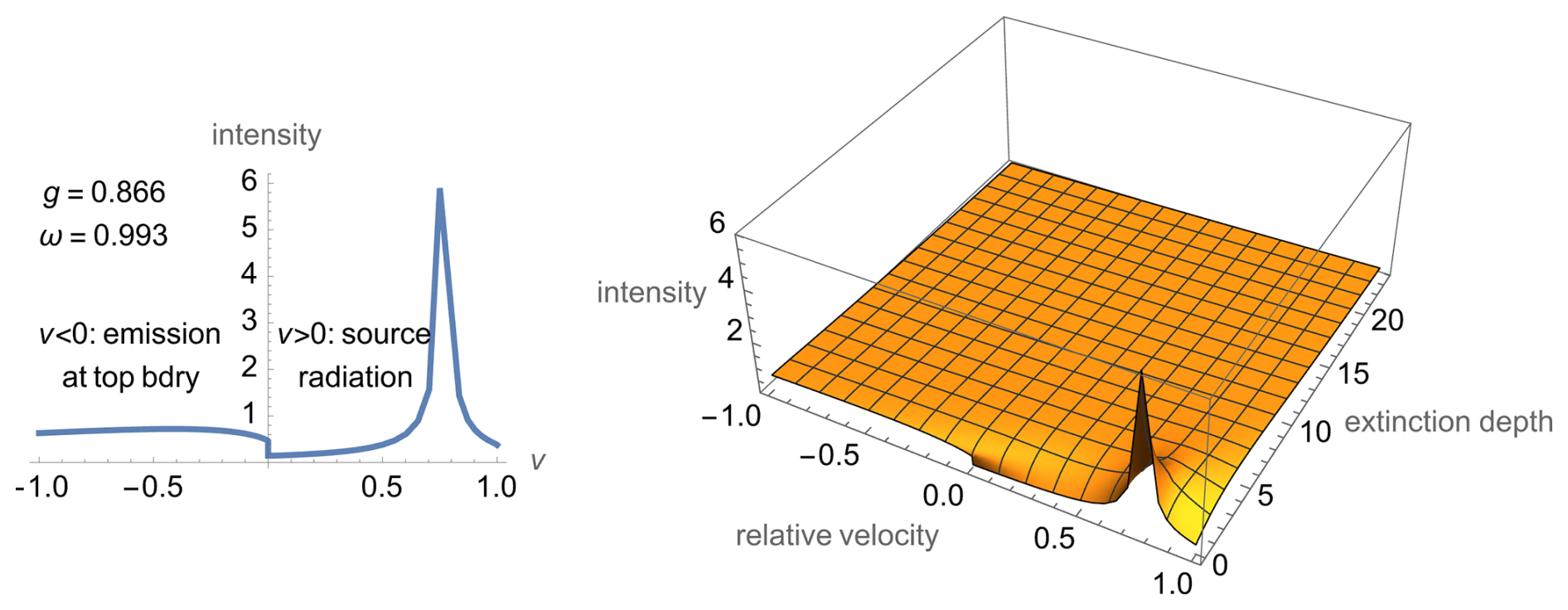
Figure 1 Intensities for strongly forwarad scattering media: (left) emission (v<0) and source (v>0) radiation. (right) internal intensities. v>0 shows particles descending deeper into the media at the different relative velocities, v<0 are light particles ascending towards the top.

Figure 1 shows the intensities for a strongly forward scattering media.

Now we turn our attention back to the basic equation Eq. (1). This can be decomposed into two parts, the direct component which is the intensity of the source rays before they are scattered or absorbed (also known as extinction), and the diffuse component which is the intensity of the scattered light. Furthermore, we can immediately determine the form of the direct component.

We accordingly define the two components of the intensity as $R(v,y,a)=e^{-y/v}s(v,a)=$ Direct intensity distribution, $M(v,y,a)=I(v,y,a)-R(v,y,a)=$ Diffuse intensity distribution.

with the boundary condition $\forall v>\mathrm{0},I(v,\mathrm{0})=s\left(v\right)$. Substituting these definitions into Eq. (1), we obtain the basic equation and side condition for the diffuse component.

$$\begin{array}{}\text{(3)}& \begin{array}{rl}M(v,y,a)& +v{\partial }_{y}M(v,y,a)-\mathit{\omega }\int K(v,w,a-b)\\ & M(w,y,b)\mathrm{d}b\mathrm{d}w=\mathit{\omega }\int K(v,w,a-b)\\ & R(w,y,b)\mathrm{d}b\mathrm{d}w\\ & \forall v>\mathrm{0},M(v,\mathrm{0},a)=\mathrm{0}\end{array}\end{array}$$

Figure 2 shows the internal direct intensity, which depends solely on the distribution of the source radiation and the extinction depth.

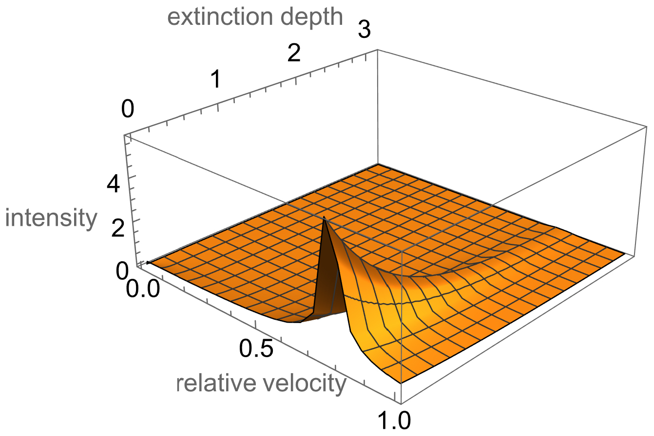
Figure 2 Internal direct intensity, showing the exponential decay of the source radiation based on the extinction depth.

Figure 3 shows the intensities for strongly forward scattering and backscattering media.

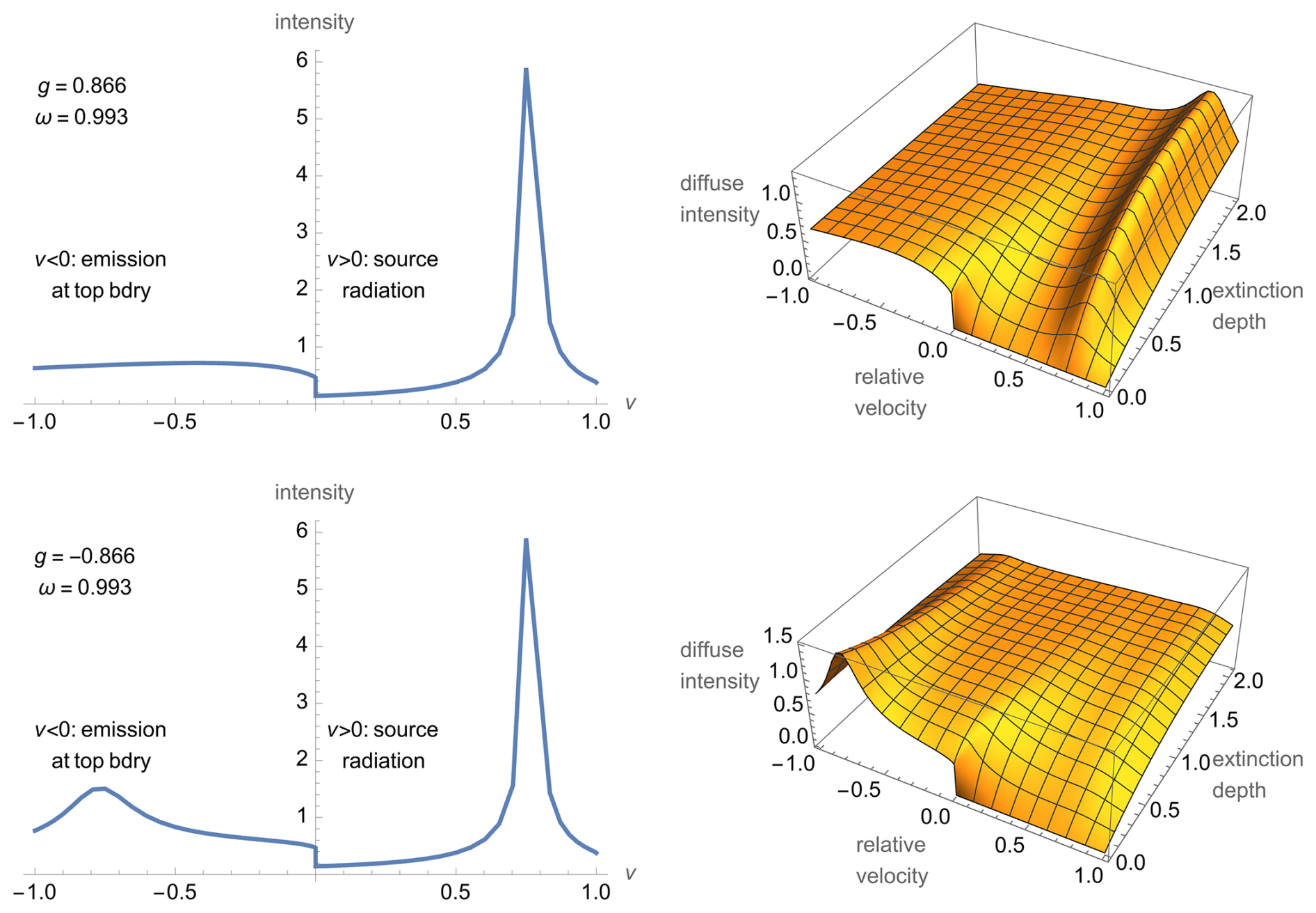
Figure 3 Internal diffuse intensities: (top) strongly forward scattering media, showing a diffuse emission and a strong internal peak at the source peak; (bottom) strongly backscattering media, showing a emission peak at the source peak, and a diffuse internal intensity.

2.3 Mesh Approximation and Galerkin's Method

We use Galerkin's method (Adjerid and Baccouch, 2010) to solve the integral equations in Eq. (3). This method uses a framework of basis functions and test functions to generate a mesh approximation for the various functions that constitute the full solution.

• v_i= Approximation points for relative velocity

• ϕ_i(v)= Basis functions

• ψ_i(v)= Test functions

• $\stackrel{\mathrm{̃}}{f}\left(v\right)=\sum f_i{\mathit{\varphi }}_i\left(v\right)=$ Approximating form for 1D functions

• $\stackrel{\mathrm{̃}}{h}(v,w)=\sum h_{ij}{\mathit{\varphi }}_i\left(v\right){\mathit{\varphi }}_i\left(w\right)=$ Approximating form for 2D functions

When seeking an approximate $\stackrel{\mathrm{̃}}{f}\left(v\right)\approx g\left(v\right)$, we expand $\stackrel{\mathrm{̃}}{f}$ and integrate both against the test functions to get the linear equation which can be solved for the approximating coefficients.

$$\forall i,\sum _j{f}_i\int {\mathit{\psi }}_i\left(v\right){\mathit{\varphi }}_j\left(v\right)\mathrm{d}v=\int {\mathit{\psi }}_i\left(v\right)g\left(v\right)\mathrm{d}v$$

Any reasonable subdivision of points can be used for v_i. In this paper, v_i will be the concatenation of two sets of the Chebyshev points, one “arc” for $-\mathrm{1}\le v\le \mathrm{0}$ and another for $\mathrm{0}\le v\le \mathrm{1}$. The basis functions ϕ_i are triangular bump functions centered on the mesh points. We will be using two different choices for test functions in the course of this paper, either

1. ψ_i=ϕ_i where the test functions are the basis functions themselves, or

2. ${\mathit{\psi }}_i\left(v\right)=\mathit{\delta }[v=v_i]$ where the test functions are the Dirac delta functions, basically defining $\stackrel{\mathrm{̃}}{f}$ by sampling it at the mesh points.

Using (2) results in equations that are simpler, faster, and frequently better conditioned than (1), but using (1) preserves more of the symmetric properties of the original problem. So we use a mixture, (1) when additional symmetry is required, and (2) when expediency dictates the use of the simpler alternative.

Applying the Galerkin approximations to the basic equations Eq. (3), we get the mesh approximations: $K(v,w;a-b)={\sum }_{jpc}{K}_{jpc}{\mathit{\varphi }}_j\left(v\right){\mathit{\varphi }}_p\left(w\right){\stackrel{\mathrm{̃}}{\mathit{\varphi }}}_c(a-b)$ is the phase function kernel, $p_{\mathrm{0}}(v;a)={\sum }_{jc}{p}_{\mathrm{0}jc}{\mathit{\varphi }}_j\left(v\right){\stackrel{\mathrm{̃}}{\mathit{\varphi }}}_c\left(a\right)$ is the intensity at surface, $M(v,y;a-b)={\sum }_{jc}{M}_{jc}\left(y\right){\mathit{\varphi }}_j\left(v\right){\stackrel{\mathrm{̃}}{\mathit{\varphi }}}_c(a-b)$ is the diffuse intensity distribution, ${\stackrel{\mathrm{̃}}{\mathit{\varphi }}}_c(a-b)={\stackrel{\mathrm{̃}}{\mathit{\varphi }}}_c(a-b+\mathrm{2}\mathit{\pi })$ is the azimuth test function.

From this we derive the finite dimensional linear ODE.

$$\begin{array}{}\text{(4)}& \begin{array}{rl}\sum _{jc}{A}_{ij}& {\stackrel{\mathrm{̃}}{B}}_{fc}{\partial }_y{M}_{jc}\left(y\right)+\sum _{jc}{B}_{ij}{\stackrel{\mathrm{̃}}{B}}_{fc}{M}_{jc}\left(y\right)\\ & -\mathit{\omega }\sum _{jpc}{B}_{ij}{\stackrel{\mathrm{̃}}{C}}_{fdc}{K}_{jpd}{B}_{pq}{M}_{qc}\left(y\right)\\ & =\mathit{\omega }\sum _{jpc}{B}_{ij}{\stackrel{\mathrm{̃}}{C}}_{fdc}{K}_{jpd}{D}_{pq}\left(y\right)p_{\mathrm{0}qc}\end{array}\end{array}$$

where $A_{ij}=\int v{\mathit{\psi }}_i\left(v\right){\mathit{\varphi }}_j\left(v\right)\mathrm{d}v$, $B_{ij}=\int {\mathit{\psi }}_i\left(v\right){\mathit{\varphi }}_j\left(v\right)\mathrm{d}v$, $C_{ij}=\int {\mathit{\varphi }}_i\left(v\right){\mathit{\varphi }}_j\left(v\right)\mathrm{d}v$, ${\stackrel{\mathrm{̃}}{B}}_{fc}=\int {\stackrel{\mathrm{̃}}{\mathit{\psi }}}_f\left(a\right){\stackrel{\mathrm{̃}}{\mathit{\varphi }}}_c\left(a\right)\mathrm{d}a$, ${\stackrel{\mathrm{̃}}{C}}_{fdc}=\int {\stackrel{\mathrm{̃}}{\mathit{\psi }}}_f\left(a\right){\stackrel{\mathrm{̃}}{\mathit{\varphi }}}_d(a-b){\stackrel{\mathrm{̃}}{\mathit{\varphi }}}_c\left(b\right)\mathrm{d}a\mathrm{d}b$, $D_{ij}\left(y\right)=\int e^{-y/v}{\mathit{\varphi }}_i\left(v\right){\mathit{\varphi }}_j\left(v\right)\mathrm{d}v$.

More succinctly,

$$\begin{array}{}\text{(5)}& A\stackrel{\mathrm{̃}}{B}{\partial }_{y}M\left(y\right)+(B\stackrel{\mathrm{̃}}{B}-\mathit{\omega }B\stackrel{\mathrm{̃}}{C}KC)M\left(y\right)=\mathit{\omega }B\stackrel{\mathrm{̃}}{C}KD\left(y\right)p_{\mathrm{0}}\end{array}$$

2.4 Conservation Properties

One of the benefits of using Galerkin's Method is that it is an orthogonal projection from the Hilbert space of differentiable functions to the Hilbert space of piece-wise continuous functions, so it preserves conservation properties under the correct weights. This includes energy conservation, reciprocity, and flux closure.

The original scattering matrix $K(v,w,a-b)$, besides being symmetric in v,w and cyclic in a−b, also satisfies the conservation condition that $\forall w,b,\iint K(v,w,a-b)\mathrm{d}a\mathrm{d}v=\mathrm{1}$. In order for the mesh approximate scattering matrix, $K(v,w;a,b)={\sum }_{jpc}{K}_{jpc}{\mathit{\varphi }}_j\left(v\right){\mathit{\varphi }}_p\left(w\right){\stackrel{\mathrm{̃}}{\mathit{\varphi }}}_c(a-b)$, to satisfy that condition, we must have

$$\begin{array}{}\text{(6)}& \forall p,b,\sum _{ja}{K}_{jpc}\underset{v=-\mathrm{1}}{\overset{v=-\mathrm{1}}{\int }}{\mathit{\varphi }}_j\left(v\right)\mathrm{d}v\underset{a=\mathrm{0}}{\overset{a=\mathrm{2}\mathit{\pi }}{\int }}{\stackrel{\mathrm{̃}}{\mathit{\varphi }}}_c(a-b)\mathrm{d}a=\mathrm{1}\end{array}$$

So the tensor ${\stackrel{\mathrm{̃}}{K}}_{jpab}=K_{jp(a-b)}$ must be doubly stochastic with respect to weights ∫ϕ_j(v)dv and $\int {\stackrel{\mathrm{̃}}{\mathit{\varphi }}}_b\left(a\right)\mathrm{d}a$. In general, the simple choice of defining the approximation by simply sampling the kernel at the mesh points, ${\stackrel{\mathrm{̃}}{K}}_{jpc}=K(v_j,w_p,a_c)$ will yield a matrix that is close to, but is not doubly stochastic.

To ensure the problem remains conservative, EigenFlux uses a variation on the Sinkhorn-Knopp algorithm (Sinkhorn and Knopp, 1967) suitable for re-scaling a matrix so that it is doubly stochastic with respect to the weights. The result is that the modified scattering matrix remains conservative in the mesh approximation.

2.5 Eigenvalue Decomposition

To solve Eq. (3), we use an eigenvalue expansion of the linear system generated by the mesh approximation.

The tensor A is near-singular at v=0, but (B−ωBKC) is diagonally dominant and non-singular. So we can look at the eigenvalue decomposition of $(B-\mathit{\omega }BKB{)}^{-\mathrm{1}}A$ for eigenvalues ν_k and eigenvectors Q_k. The resulting ODE becomes

$$\begin{array}{}\text{(7)}& {\mathit{\nu }}_k{\partial }_y{\mathit{\mu }}_k\left(y\right)+{\mathit{\mu }}_k\left(y\right)={\mathit{\rho }}_k\left(y\right)\end{array}$$

where ν_k,Q_k Eigenvalues and eigenvectors, μ_k(y) Eigenvector decomposition of M_j(y), ρ_k(y) Transformed boundary data, and $A{Q}_k={\mathit{\nu }}_k(B-\mathit{\omega }BKC)Q_k$, $M_j\left(y\right)={\sum }_k{Q}_k{\mathit{\mu }}_k\left(y\right)$, ${\mathit{\rho }}_k\left(y\right)=\mathit{\omega }{Q}^{-\mathrm{1}}(B-\mathit{\omega }BKC{)}^{-\mathrm{1}}BKD(y)s$.

Figure 4 shows the computed eigenvalues for varying parameter values. In general, there will be a continuous spectrum from −1 to 1, plus isolated eigenvalues at $v=\pm \mathrm{1}$ that correspond to the limiting distribution at increasing depths. Figure 5 shows the computed eigenvectors for a single set of the parameter values. Note in particular the all-positive eigenvectors for $\mathit{\nu }=\pm \mathrm{1.8}$. These are the limiting distributions of the intensity.

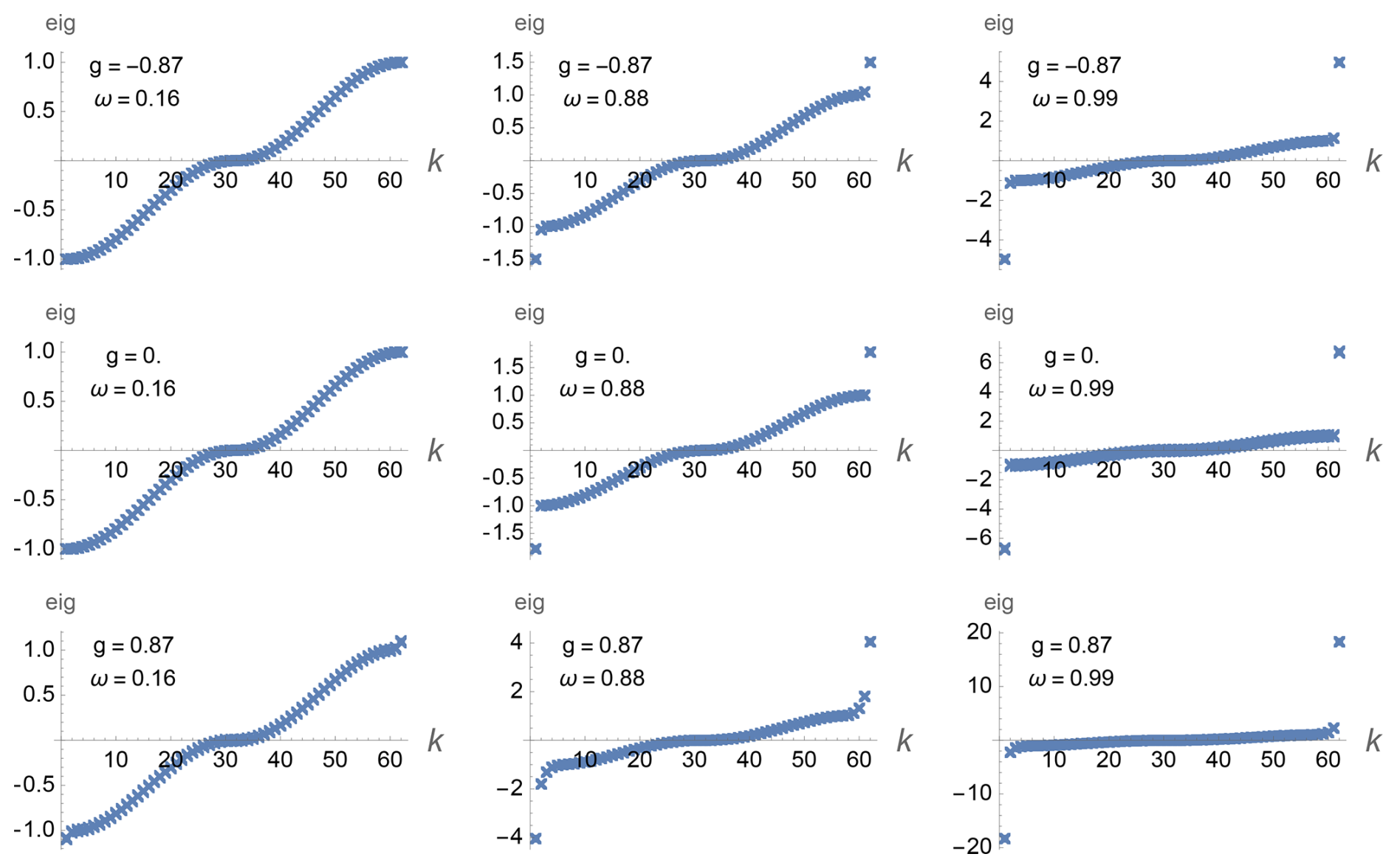
Figure 4 Eigenvalues for varying values of asymmetry g and scatter fraction ω, showing a continuous spectrum from $v=-\mathrm{1}$ to v=1 and two isolated eigenvalues. Note that the absolute value of the isolated eigenvalues increases with increasing ω.

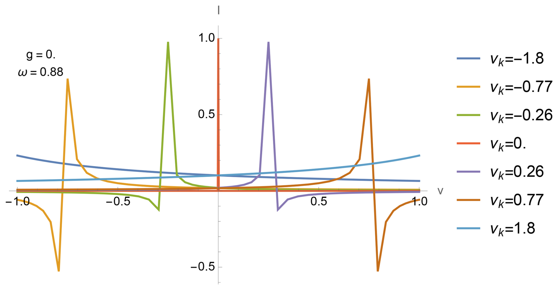
Figure 5 Sampling of eigenvectors for a single run. The eigenvectors for the isolated eigenvalues show as all-positive. The eigenvectors for the continuous spectrum are delta functions around the various relative velocities of the mesh.

We now have decomposed the problem into a set of one-dimensional first-order linear ODEs which have the general solution form

$$\begin{array}{}\text{(8)}& {\mathit{\mu }}_k\left(y\right)={\mathit{\mu }}_k\left(\mathrm{0}\right)e^{-y/{\mathit{\nu }}_k}+(\mathrm{1}/{\mathit{\nu }}_k)\underset{\mathrm{0}}{\overset{y}{\int }}{e}^{(\mathit{\eta }-y)/{\mathit{\nu }}_k)}{\mathit{\rho }}_k\left(\mathit{\eta }\right)\mathrm{d}\mathit{\eta }\end{array}$$

There are additional considerations when the eigenvalue is zero or negative.

One of the eigenvalues will be close to (or equal to) 0. In this case, we go back to Eq. (7) and use the resulting condition μ_k(y)=ρ_k(y).

When the eigenvalue is negative, Eq. (8) would imply that we have an unstable mode. In this case, we can apply the natural reflectance assumption discussed previously to the new ODEs.

With these considerations, we have the following more specific solution.

$$\begin{array}{}\text{(9)}& \begin{array}{rl}{\mathit{\nu }}_k>\mathrm{0}& \Rightarrow {\mathit{\mu }}_k\left(y\right)={\mathit{\mu }}_k\left(\mathrm{0}\right)e^{-y/{\mathit{\nu }}_k}+(\mathrm{1}/{\mathit{\nu }}_k)\underset{\mathrm{0}}{\overset{y}{\int }}{e}^{(\mathit{\eta }-y)/{\mathit{\nu }}_k)}{\mathit{\rho }}_k\left(\mathit{\eta }\right)\mathrm{d}\mathit{\eta }\\ {\mathit{\nu }}_k=\mathrm{0}& \Rightarrow {\mathit{\mu }}_k\left(y\right)={\mathit{\rho }}_k\left(y\right)\\ {\mathit{\nu }}_k<\mathrm{0}& \Rightarrow {\mathit{\mu }}_k\left(y\right)=-(\mathrm{1}/{\mathit{\nu }}_k)\underset{y}{\overset{\mathrm{\infty }}{\int }}{e}^{(\mathit{\eta }-y)/{\mathit{\nu }}_k)}{\mathit{\rho }}_k\left(\mathit{\eta }\right)\mathrm{d}\mathit{\eta }\end{array}\end{array}$$

Note in particular that this implies that for $k:{\mathit{\nu }}_k\le \mathrm{0}$, μ_k(0) is determined by ρ_k (and hence by p₀). For positive ν_k, determination of μ_k(0) is slightly more complicated – they are determined by taking the side-condition $v>\mathrm{0}\Rightarrow M(v,\mathrm{0})=\mathrm{0}$ (see Eq. 3), expanding by $M_j\left(\mathrm{0}\right)={\sum }_k{Q}_k{\mathit{\mu }}_k\left(\mathrm{0}\right)$ (see Eq. 7) and solving for the unknown μ_k(0).

2.6 Block Circulant

The eigenvalue decomposition of $\stackrel{\mathrm{̃}}{R}=(B\stackrel{\mathrm{̃}}{B}-\mathit{\omega }B\stackrel{\mathrm{̃}}{C}KB{)}^{-\mathrm{1}}A\stackrel{\mathrm{̃}}{B}$ can be computationally costly. However, note that all functions/matrices (other than p₀(v,a)) that are dependent on azimuth are cyclically symmetric. As a result, the tensor $\stackrel{\mathrm{̃}}{R}$ has some special properties:

1. $\stackrel{\mathrm{̃}}{R}$ is block circulant, thus ${\stackrel{\mathrm{̃}}{R}}_{fcij}={\stackrel{\mathrm{̃}}{R}}_{(f-c)\mathrm{0}ij}$

2. The individual blocks of $\stackrel{\mathrm{̃}}{R}$ are symmetric, implying that ${\stackrel{\mathrm{̃}}{R}}_{ij}^{fc}={\stackrel{\mathrm{̃}}{R}}_{ji}^{fc}$

Because of (1) and (2), the eigenvalues and eigenvectors of $\stackrel{\mathrm{̃}}{R}$ are real and can be determined from the number of blocks and the eigenvalue decomposition of a geometric sum of the individual blocks (Tee, 2007, 1963; Davis, 1979). Let the blocks of $\stackrel{\mathrm{̃}}{R}$ be given by R_i−j. Let ρ be a primitive root of unity of order n, the number of blocks, so that ρⁿ=1 and such that {ρⁱ} generates a complete list of all roots of unity of order n. Let $H\left(\mathit{\rho }\right)={\sum }_j{\mathit{\rho }}^j{R}_{n-j}$. Then the eigenvalues of $\stackrel{\mathrm{̃}}{R}$ are the n⋅m eigenvalues of H(ρ^k), and the eigenvectors are the outer product of $\mathit{\left\{}{\mathit{\rho }}_k^j\mathit{\right\}}$ and the eigenvectors of H(ρ^k).

2.7 Depth Model Approximation

Finding a good approximation mesh for the depth y can be problematic because y has an unbounded range, so instead we use the exponential depth z where $z=e^{-y}$, $\mathrm{0}\le z\le \mathrm{1}$ so that for a function of depth f(y) we have $f\left(y\right)=f(-\ln (z\left)\right)$.

Similar to Step One, we apply the following mesh approximation to Eq. (9), (but now with ${\overline{\mathit{\psi }}}_i\left(z\right)=\mathit{\delta }[z=z_i]$, option (2) in the discussion on Mesh Approximation).

2.7.1 Depth Model

• ${\mathit{\mu }}_k\left(y\right)={\sum }_m{\mathit{\mu }}_{km}{\mathit{\varphi }}_m\left(z\right)$ Transformed intensity

• ${\mathit{\rho }}_k\left(z\right)={\sum }_m{\mathit{\rho }}_{km}{\mathit{\varphi }}_m\left(z\right)$ Transformed boundary conditions

• ${\mathit{\rho }}_{kh}=\mathit{\omega }{Q}^{-\mathrm{1}}(B-\mathit{\omega }BKB{)}^{-\mathrm{1}}BKD(z_h)p_{\mathrm{0}}$

• $D_{ij}\left(z\right)=\int z^{\mathrm{1}/v}{\mathit{\varphi }}_i\left(v\right){\mathit{\varphi }}_j\left(v\right)\mathrm{d}v$

From this and Eq. (9) we get the following.

$$\begin{array}{rl}{\mathit{\nu }}_k>\mathrm{0}& \Rightarrow {\mathit{\mu }}_{km}={\mathit{\mu }}_{\mathrm{0}k}{z}_m^{\mathrm{1}/{\mathit{\nu }}_k}+(\mathrm{1}/{\mathit{\nu }}_k){\mathit{\rho }}_{km}\\ & \underset{z_m}{\overset{\mathrm{1}}{\int }}{z}_m^{-\mathrm{1}}(z_m/\mathit{\zeta }{)}^{\mathrm{1}+\mathrm{1}/{\mathit{\nu }}_k}{\mathit{\varphi }}_m(\mathit{\zeta })d\mathit{\zeta }\\ {\mathit{\nu }}_k=\mathrm{0}& \Rightarrow {\mathit{\mu }}_{km}={\mathit{\rho }}_{km}\\ {\mathit{\nu }}_k<\mathrm{0}& \Rightarrow {\mathit{\mu }}_{km}=-(\mathrm{1}/{\mathit{\nu }}_k){\mathit{\rho }}_{km}\underset{\mathrm{0}}{\overset{z_m}{\int }}{z}_m^{-\mathrm{1}}(z_m/\mathit{\zeta }{)}^{\mathrm{1}+\mathrm{1}/{\mathit{\nu }}_k}{\mathit{\varphi }}_m(\mathit{\zeta })\mathrm{d}\mathit{\zeta }\end{array}$$

This allow us to compute μ and M under the natural reflectance assumption.

2.8 Satisfying the General Two-Boundary Problem

The boundary conditions for a two-boundary radiative transfer problem specify the downward sources of illumination at the top boundary, and the upward sources of illumination at the bottom boundary.

• $I(w_j,\mathrm{0})=r_{\mathrm{0}}\left(w_j\right)=$ downwards illumination at top boundary (w_j≥0)

• $I(w_j,b)=r_b\left(w_j\right)=$ upwards illumination at bottom boundary (w_j≤0)

The general solution for radiative transfer for a medium with finite depth and two boundaries, top and bottom, can be expressed as the linear combination of the one-boundary solution for the top boundary with the one-boundary solution for the bottom boundary.

Let Φ be the fundamental solution for Eq. (3), so that M=Φp₀. To simplify the notation, we replace the indices by the underlying mesh points e.g. $M_i\left(y\right)=M(v_i,y)$. We then note that the solution for a system with a bottom boundary is given by a depth-reversal of the solution for a system with a top boundary.

$$\begin{array}{}\text{(10)}& \begin{array}{rl}{\stackrel{\mathrm{̃}}{M}}^{\mathrm{top}}(v_i,y)& =\sum _{w_j\ge \mathrm{0}}\mathrm{\Phi }(v_i,w_j,y)r_{\mathrm{0}}\left(w_j\right)\\ {\stackrel{\mathrm{̃}}{M}}^{\mathrm{bot}}(v_i,y)& =\sum _{w_j\le \mathrm{0}}{}^R\mathrm{\Phi }(v_i,w_j,b-y)r_b\left(w_j\right)\\ {}^R\mathrm{\Phi }(v_i,w_j,b-y)& =\mathrm{\Phi }(-v_i,-w_j,b-y)\end{array}\end{array}$$

where b is the depth of bottom boundary, ${\stackrel{\mathrm{̃}}{M}}^{\mathrm{top}}$ is the solution to top-boundary problem under natural reflectance assumption, ${\stackrel{\mathrm{̃}}{M}}^{\mathrm{bot}}$ is the solution to bottom boundary problem under natural reflectance assumption, ^RΦ is the depth-reversed fundamental solution, r₀(w_j) is the downwards illumination of top boundary (w_j≥0), r_b(w_j) is the upwards illumination of bottom boundary (w_j≤0).

Both the downwards and upwards system satisfy the base integro-differential equation Eq. (3). A linear combination of the two sets of solutions has the same degrees of freedom as the two-boundary problem, so a linear combination of the two will span the solution set.

To find that solution, first let's decompose the systems into downwards flows (v≥0) and upwards flows (v≤0).

$$\left[\begin{array}{c}{I}_y^{\uparrow }\\ I_y^{\downarrow }\end{array}\right]=\left[\begin{array}{lcc}{}^R{\mathrm{\Phi }}_{b-y}^{\downarrow }& & {\mathrm{\Phi }}_y^{\uparrow }\\ {}^R{\mathrm{\Phi }}_{b-y}^{\uparrow }& & {\mathrm{\Phi }}_y^{\downarrow }\end{array}\right]\left[\begin{array}{c}{r}_b^{\uparrow }\\ r_{\mathrm{0}}^{\downarrow }\end{array}\right]$$

where $I_y^{\uparrow }$ is the Intensity of flow upwards at depth y, $I_y^{\downarrow }$ is the Intensity of flow downwards at depth y.

From this we can determine the boundary input and output flows.

$$\left[\begin{array}{c}{S}_b^{\uparrow }\\ S_{\mathrm{0}}^{\downarrow }\end{array}\right]=\left[\begin{array}{lcc}{}^R{\mathrm{\Phi }}_{\mathrm{0}}^{\downarrow }& & {\mathrm{\Phi }}_b^{\uparrow }\\ {}^R{\mathrm{\Phi }}_b^{\uparrow }& & {\mathrm{\Phi }}_{\mathrm{0}}^{\downarrow }\end{array}\right].\left[\begin{array}{c}{r}_b^{\uparrow }\\ r_{\mathrm{0}}^{\downarrow }\end{array}\right]$$

$$\left[\begin{array}{c}{O}_{\mathrm{0}}^{\uparrow }\\ O_b^{\downarrow }\end{array}\right]=\left[\begin{array}{lcc}{}^R{\mathrm{\Phi }}_b^{\downarrow }& & {\mathrm{\Phi }}_{\mathrm{0}}^{\uparrow }\\ {}^R{\mathrm{\Phi }}_{\mathrm{0}}^{\uparrow }& & {\mathrm{\Phi }}_b^{\downarrow }\end{array}\right].\left[\begin{array}{c}{r}_b^{\uparrow }\\ r_{\mathrm{0}}^{\downarrow }\end{array}\right]$$

And so we have found the two-boundary system.

$$\left[\begin{array}{c}{O}_{\mathrm{0}}^{\uparrow }\\ O_b^{\downarrow }\end{array}\right]=\left[\begin{array}{lcc}{}^R{\mathrm{\Phi }}_b^{\downarrow }& & {\mathrm{\Phi }}_{\mathrm{0}}^{\uparrow }\\ {}^R{\mathrm{\Phi }}_{\mathrm{0}}^{\uparrow }& & {\mathrm{\Phi }}_b^{\downarrow }\end{array}\right].{\left[\begin{array}{lcc}{}^R{\mathrm{\Phi }}_{\mathrm{0}}^{\downarrow }& & {\mathrm{\Phi }}_b^{\uparrow }\\ {}^R{\mathrm{\Phi }}_b^{\uparrow }& & {\mathrm{\Phi }}_{\mathrm{0}}^{\downarrow }\end{array}\right]}^{-\mathrm{1}}.\left[\begin{array}{c}{S}_b^{\uparrow }\\ S_{\mathrm{0}}^{\downarrow }\end{array}\right]$$

where $S_b^{\uparrow }$ is the Intensity of source input at bottom boundary at depth b, $S_{\mathrm{0}}^{\downarrow }$ is the Intensity of source input at top boundary at depth 0, $O_{\mathrm{0}}^{\uparrow }$ is the Intensity of output from top boundary, $O_b^{\downarrow }$ is the Intensity of output from bottom boundary boundary.

3 Results

3.1 Numerical Investigations of Analytical Features

For the numerical experiments, the mesh approximation for the relative velocity v have 61 sample points distributed as two arcs of shifted Chebeyshev points, to give additional resolution around the three points $v=-\mathrm{1},\mathrm{0},\mathrm{1}$. The mesh approximation for the scaled depths $\mathrm{0}\le z\le \mathrm{1}$ has 67 sample points distributed as shifted Chebeyshev points to provide additional resolution at $y=\mathrm{0},\mathrm{\infty }$. The actual scaling used is $z=e^{-y/{\widehat{y}}_{\mathrm{05}}}$ where ${\widehat{y}}_{\mathrm{05}}$ is the two-stream estimate of the depth at which the transmission was reduced to 5 % of the original source. This provides better resolution by the numerical algorithm when the test case has strong forward scattering or a significant backward scattering component.

The test cases used the Henyey-Greenstein phase function parametrized by g the asymmetry parameter, which in this case is equal to the average scatter angle relative to an incident angle.

The 957 test cases used all pairs of 33 values of the asymmetry parameter (g= average scattering angle) and 29 values of the scattering fraction (ω= probability of scatter given extinction $=\mathrm{1}-$ probability of absorption given extinction).

Table 1 Test case parameters. v_i and z_i were fixed for all runs, so there were 33×29 test cases. These test cases span the range of asymmetry and single stage albedo, with increased density at the extremes of strong scattering and low absorption, in order to cover the analytic features of the RTM. For v and z Chebyshev point of the second kind were used, remapped to the interval [0,1] (and [−1,0] for v.) Then g is distributed as the remapped Chebyshev points of the first kind. The strong sensitivity to low absorption dictated that ω be the squares of the Chebyshev points of the first kind.

Table 1 shows the parameters for the test cases. The Fortran implementation took 0.0742 s per test case, the Python implementation took 2.45 s per test case, and the Mathematica implementation took 23.5 s per test case. More detailed timing studies are presented below.

3.2 The Asymptotic Radiance Distribution

Observations of radiance in deep waters show that the shape of the radiance distribution approaches a limiting distribution, and the rate of decay of that distribution is exponential (Mobley, 1994). This is the asymptotic radiance distribution, and the exponent of decay is the diffusion exponent (Van De Hulst, 1980). The max eigenvalue of Eq. (5) is the diffusion exponent.

As shown in Figs. 4 and 5 and discussed below, each material has a unique largest eigenvalue ν greater than 1 and a unique positive eigenvector. The rate of attenuation for each eigenvector is the reciprocal of the corresponding eigenvalue, so this positive eigenvector has the slowest rate of attenuation among the diffuse components of the intensity. Since the largest eigenvalue is also greater than 1, it's rate of attenuation is also slower than the rate of attenuation of the direct component.

Hence the positive eigenvector represents the asymptotic limit of the distribution of the intensity as the optical depth increases, and the rate of convergence is given by the reciprocal of the eigenvalue. As shown in Fig. 6, the maximum eigenvalue (and hence the slowest decay in diffusion) increases as absorption decreases (ω→1) and as the forward scattering ratio increases (g→1). So the diffuse intensity decays slower than the extinction decay of the direct intensity.

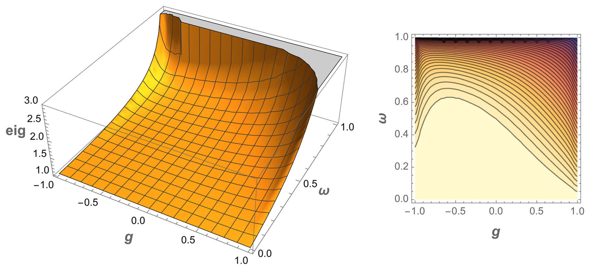
Figure 6 Maximum eigenvalues for varying asymmetry g and scatter fraction ω. The maximums increase as ω increases, i.e. as absorption decreases.

However the maximum eigenvalue is close to one on the majority of the region. Such materials have a decay rate of diffusion very close to the extinction decay rate of the direct component, so are in a strong sense effectively transparent in that there is always a component of direct intensity relative to the diffuse intensity. Given the direct component source, Fig. 7 shows the convergence of an opaque material to the diffusion limit, while Fig. 8 shows a semi-transparent material where the direct component remains larger than the limiting diffuse component.

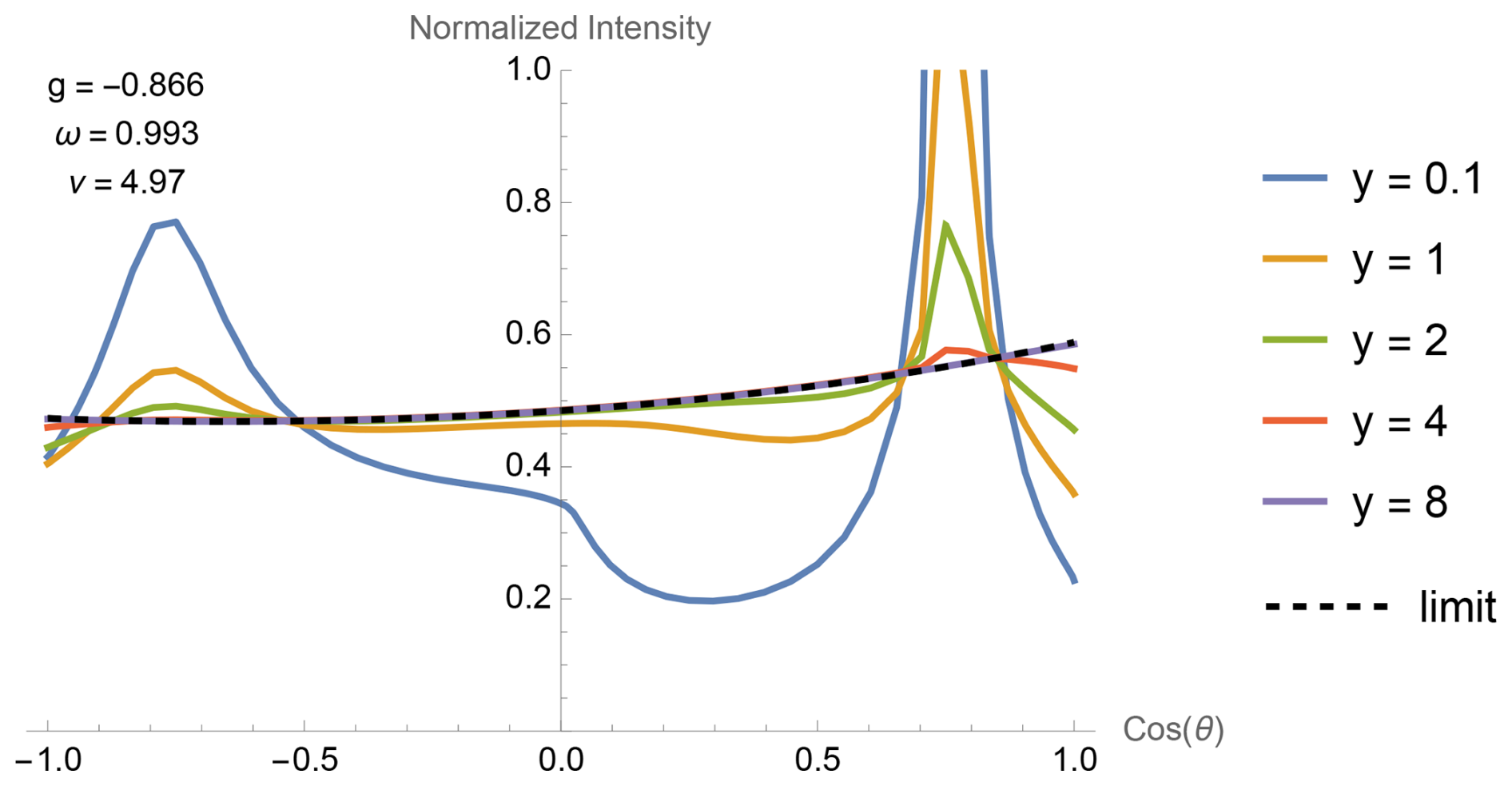
Figure 7 Asymptotic radiance distribution for a low absorption media (ω=0.993). As depth y increases, the diffuse internal intensity dominates the direct source intensity (the peak at the right) and the normalized intensity converges to the diffusion limit.

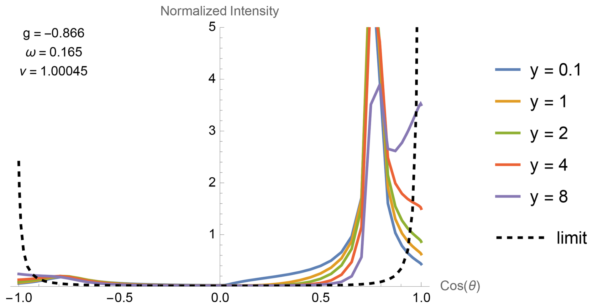
Figure 8 Asymptotic radiance distribution as depth y increases for a high absorption media (ω=0.165). The direct source intensity (the peak at the right) dominates the diffuse limit.

3.3 Comparing Apparent Optical Properties to Two-Stream Approximation

The two-stream/Kubelka-Munk formulation provides simple analytic formulas for computing g and ω from R and η, and for the inverse. We use it as a reference baseline in our investigation of the properties of the multi-stream formulation.

The Inherent Optical Properties (IOP) are the properties of a media that characterize its optical behavior (Mobley, 1994). For Eq. (1) they consist of the optical depth, the scatter fraction, and the scattering matrix. Since the numerical investigations here assume normalization by the optical depth and use the Henyey-Green one-parameter phase function, it is sufficient to use the scattering asymmetry g and the scattering fraction ω. This is also the common practice when using a two-stream approximation such as the Kubelka-Munk formulation. The Apparent Optical Properties (AOP) are the observed optical properties of a media (Mobley, 1994). Following common practice, we look at the measured reflectance R and attenuation coefficient η.

Figure 9 shows the reflectance and the attenuation coefficient at an optical depth of 0.75 for (a) g=0.85 as ω varies from −1 to 1, (b) $\mathit{\omega }=-\mathrm{1}$ as g varies from 0 to 1, and (c) ω=1 as g varies from 0 to 1, for the numerical simulation and for the two-stream analytic approximation.

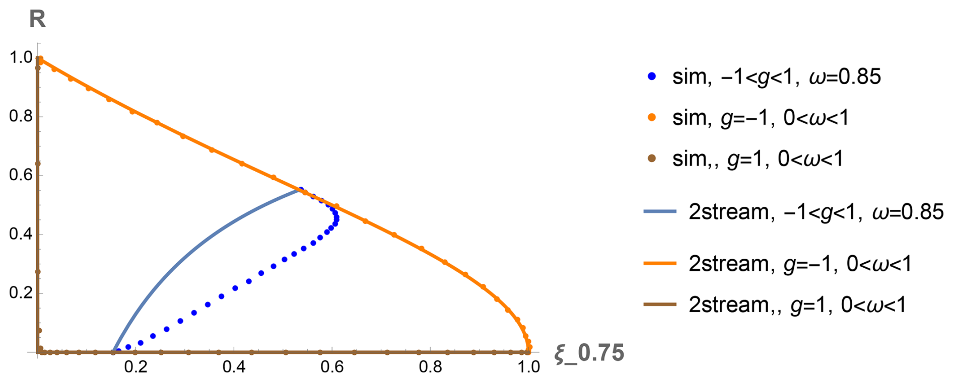
Figure 9 Reflectance and Attenuation Coefficient at 0.75 loss depth as computed by simulation and as given by the Kubelka-Munk two-stream approximation. There is agreement on the borders when $g=\pm \mathrm{1}$, but significant devation in the interior when $-\mathrm{1}<g<\mathrm{1}$.

This illustrates the following:

1. The two-stream approximation agrees with the full system on the four boundaries, $\mathit{\omega }=\pm \mathrm{1}$ and $g=\mathrm{0},\mathrm{1}$,

2. Overall error of the two-stream approximation is ≈0.15.

3. The reflectance R and attenuation coefficient ξ₇₅ (at transmission loss 0.75) do not uniquely determine the asymmetry g and scatter fraction ω for $g<-\mathrm{0.7}$.

If we look at the scatter diagrams at differing transmission loss depths in Fig. 10, we see that the difficulty of invertibility increases as the loss increases, the data lets us determine g and ω at loss depths of less than 50 %, or for $g>-\mathrm{0.5}$, while inversion becomes problematic for loss depths greater than 75 % and $g<-\mathrm{0.7}$.

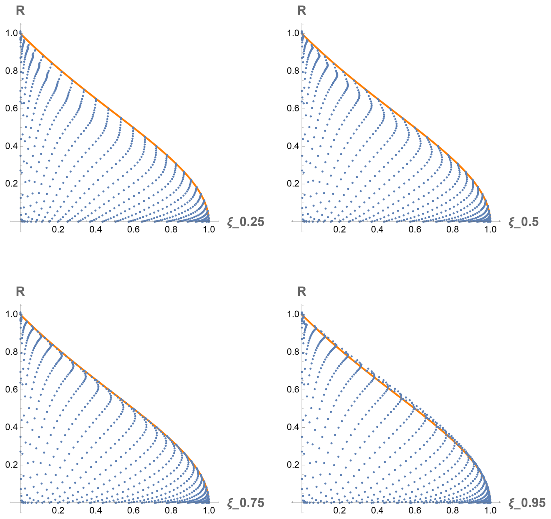
Figure 10 Scatter diagrams for reflectance R and attenuation coefficient ξ at loss depths of 25 %, 50 %, 75 %, and 95 %.

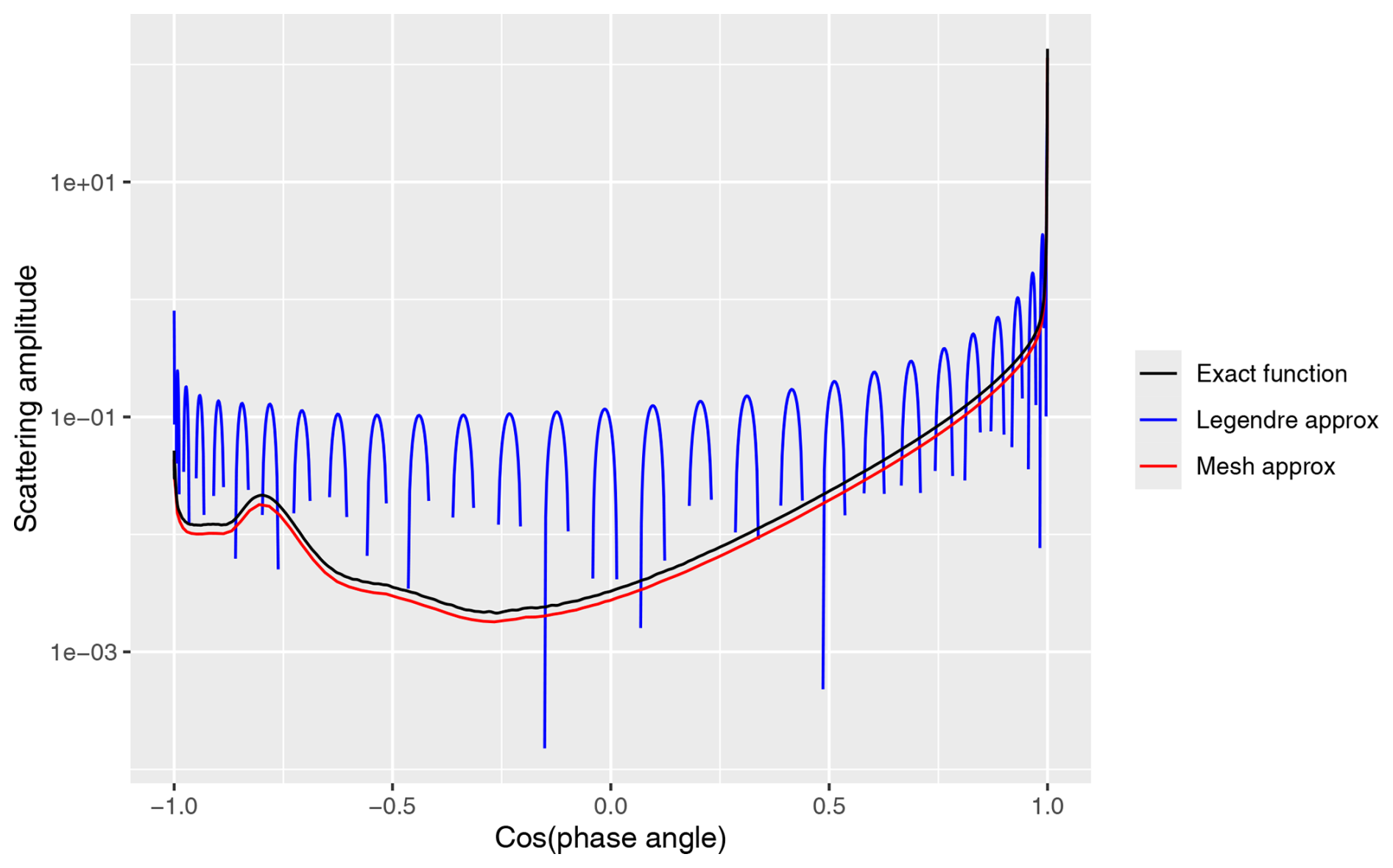
Figure 11 Cloud phase function and approximations for n=56. The original phase function is strongly forward scattering, but also has a significant backward scattering component. The gaps in the Legendre approximation are due to the approximation going negative.

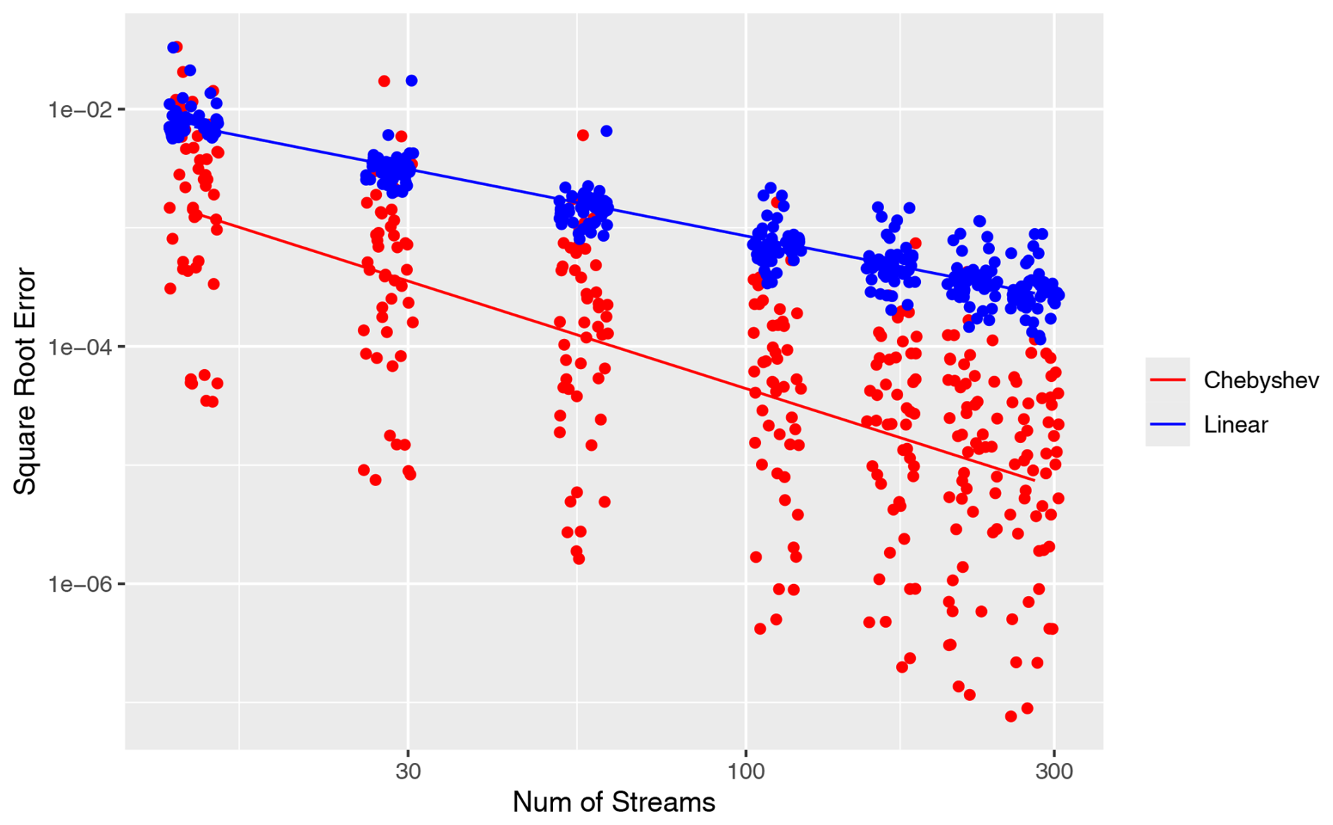
Figure 12 Error as a function of number of streams for Chebyshev spacing and for linear spacing, plotted on a log-log scale. The error is the integration of the squared error between the intensity and its reference equation. Fitting was made to a log-log curve. Jitter added to number of streams to expand point cloud.

3.4 Comparison to Other Models

A choice was made as to which Radiative Transfer Models (RTMs) to compare against EigenFlux (See Table 2). The major concerns were: (1) Does the RTM explicitly model scattering? (2) Does the RTM include the visible spectrum? (3) Is it available as open access, and is it still supported? (4) Does it use its own solver or does it use a different RTM? (5) Is it mature (version >1.0)?

These considerations led to two RTMS: DISORT and MYSTIC, of which DISORT was chosen due to its long maturity and the multiple RTMs that use it as their solver.

Table 2 Radiative Transfer Models (RTMs) considered in course of study. Does not include RTMs intended for spectrographic use which only implicitly consider multiple scattering. Does not include models that use other models as their solver. Includes only mature (version >1.0) models under active support. List of models obtained from Wikipedia (Wikipedia, 2026) and an independent literature search.

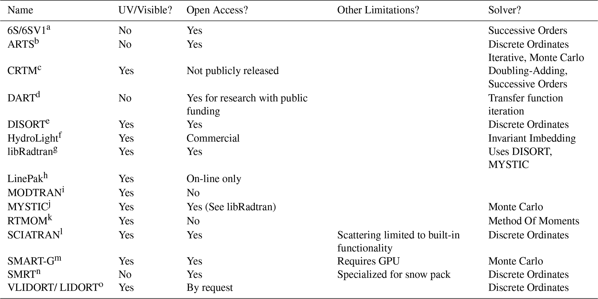
^a 6S/6SV1, “Second Simulation of a Satellite Signal in the Solar Spectrum vector code”, https://salsa.umd.edu/6spage.html (last access: 6 May 2026). ^b ARTS, “The Atmospheric Radiative Transfer Simulator”, https://www.radiativetransfer.org/about/ (last access: 6 May 2026). ^c CRTM, “Community Radiative Transfer Model (CRTM)”, https://www.jcsda.org/jcsda-project-community-radiative-transfer-model (last access: 6 May 2026). ^d DART, “The Discrete Anisotropic Radiative Transfer Model”, https://dart.omp.eu/#/ (last access: 6 May 2026). ^e DISORT, “LLLab DISORT Website”, http://www.rtatmocn.com/disort/ (last access: 6 May 2026). ^f HydroLight, “HydroLight”, https://www.numericaloptics.com/hydrolight.html (last access: 6 May 2026). ^g libRadtran, “libradtran”, https://www.libradtran.org/doku.php (last access: 6 May 2026). ^h LinePak, “Spectral Calc.com: High-resolution spectral modeling”, https://www.spectralcalc.com/info/about (last access: 6 May 2026). ⁱ MODTRAN, “MODTRAN®”, http://modtran.spectral.com (last access: 6 May 2026). ^j MYSTIC, “MYSTIC – the Monte Carlo code for the physically correct tracing of photons in cloudy atmospheres”, http://www.bmayer.de/index.html?mystic.html&1 (last access: 6 May 2026). ^k RTMOM, “Radiative Transfer Model Comparison with Satellite Observations over CEOS Calibration Site Libya-4”, https://www.mdpi.com/2073-4433/13/11/1759 (last access: 6 May 2026). ^l SCIATRAN, “SCIATRAN: RADIATIVE TRANSFER MODEL AND RETRIEVAL ALGORITHM”, https://www.iup.uni-bremen.de/sciatran/ (last access: 6 May 2026). ^m SMART-G, “SMART-G: a Monte Carlo GPU Radiative Transfer code”, https://hygeos.com/en/smart-g/ (last access: 6 May 2026). ⁿ SMRT, “SMRT: Snow Microwave Radiative Transfer model”, https://smrt-model.science (last access: 6 May 2026). ^o VLIDORT/LIDORT, “Overview of RT Solutions Products”, http://www.rtslidort.com/about_overview.html (last access: 6 May 2026).

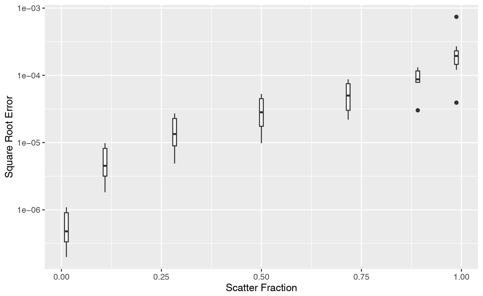
Figure 13 Boxplot of EigenFlux error as a function of scatter fraction. Data is for the run with nn=168. Lower absorption increases error.

3.5 Phase Function Limitations

Of the tools considered, the snow and ice models are intended for highly forward scattering problems. Since they use the DO method, they are subject to the instability problems that come with using Legendre expansions of a highly asymmetric phase function. They ameliorate those problems with the use of variations on a specific technique, called the δ−N method in Thomas and Stamnes (1999), which treat forward scattering light particles as non-scattering transmitted particles. But as we see below in Fig. 16, the effect of this is limited.

Stamnes et al. (2011) report that while snow grains have asymmetry g=0.9, brine pockets have asymmetry g=0.997. Their tool, CASIO-DISORT, derived from DISORT, was limited practically to g_max≤0.9. The higher g required for brine-snow mixtures was achieved through a reduced forward scattering transformation which is essentially an externally applied δ−N method.

We can see some of the advantages of the mesh approximation over the Legendre decomposition in managing phase functions. Figure 11 shows the approximations of the cloud phase function defined in Garcia and Siewert (1985), which contains both strongly forward scattering and a significant backward scattering component. Approximations used are those used in the case of n=56 streams.

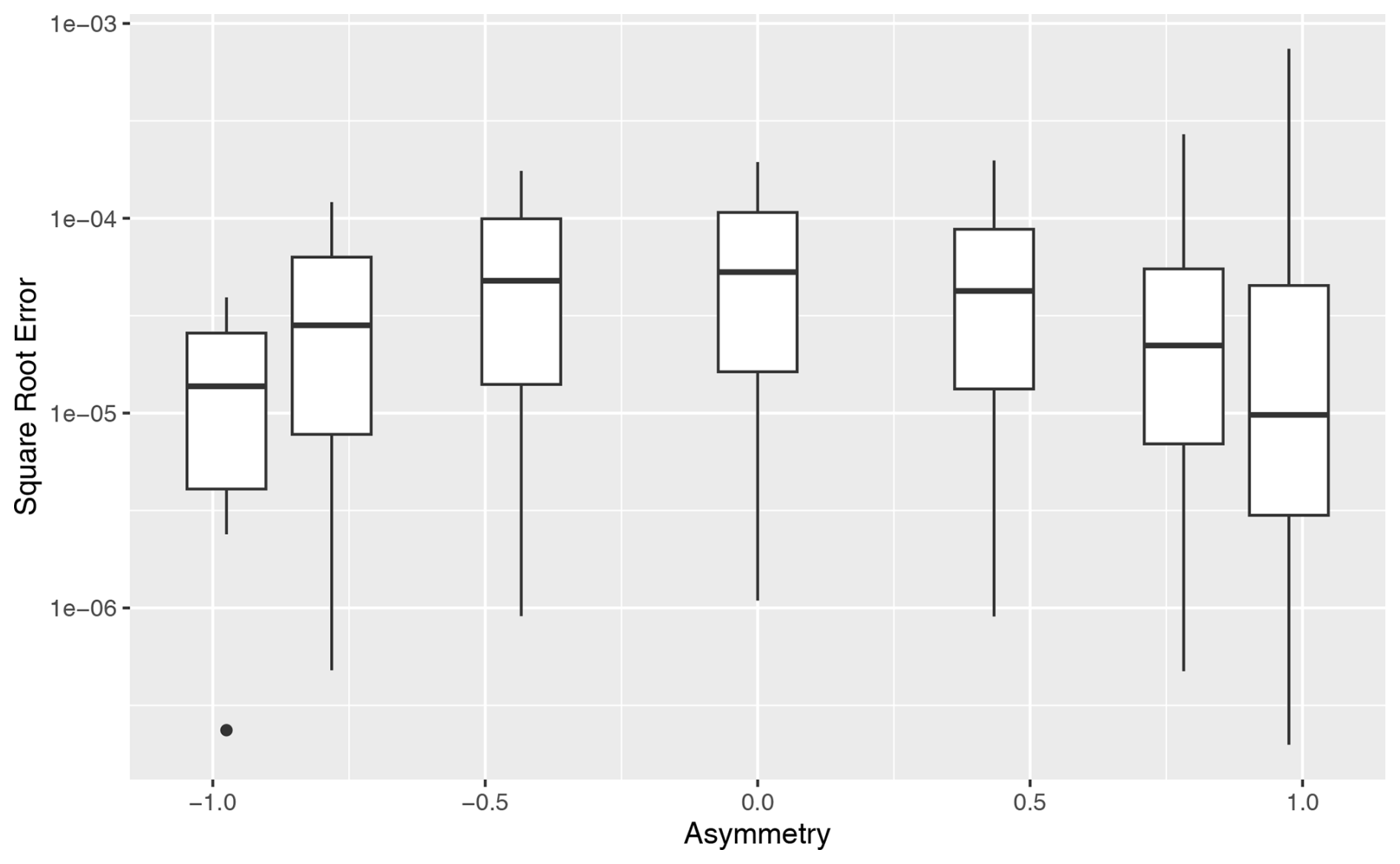
Figure 14 Boxplot of EigenFlux error as a function of asymmetry. Data is for the run with nn=168. Strong asymmetry decreases error slightly.

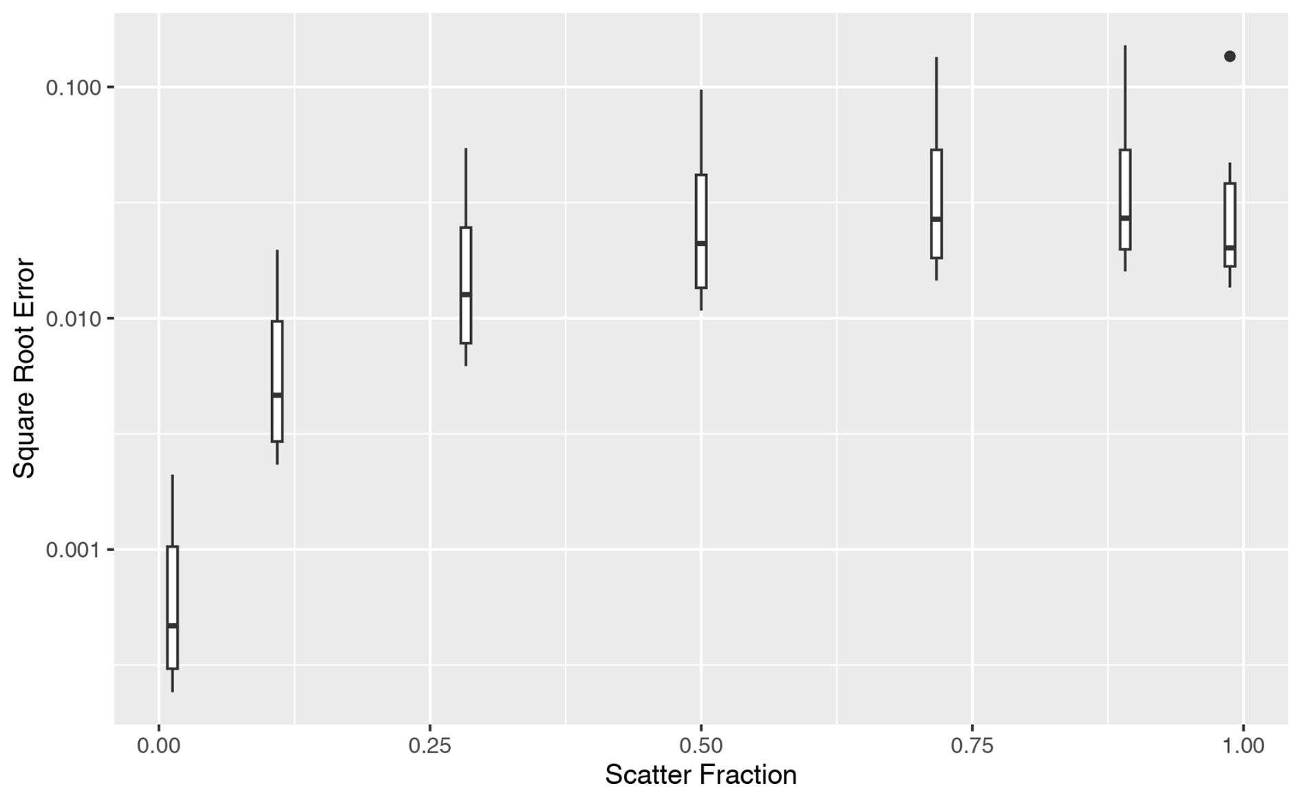
Figure 15 Boxplot of DISORT error as a function of scatter fraction. Data is for the run with nn=168. Lower absorption increases error.

3.6 Accuracy and Timing Studies

To establish the accuracy of the EigenFlux algorithm, numerical investigations were conducted on a MacBook Pro with 2.6 GHz 6-Core Intel Core i7, 16Gb of RAM, running Tahoe V26.3.1. The final algorithm was coded in GNU Fortran 2008. The accuracy of the implementation was first verified by hand comparisons to published tables (see Table 35 in Van De Hulst, 1980).

The distribution for DISORT4 was downloaded from the Light and Life Lab website (LLLab, 2023), along with its standard test suite, and compiled with the same compiler and options as Eigenflux was.

To provide a more general coverage of accuracy over a range of conditions, the error between the computed solution and the reference equation was computed. The integral formulation Eq. (2) was used as the reference equation because it is a numerically stable exact form. A Schlick phase distribution (Blasi et al., 1993; Pharr and Humphreys, 2004) was used as the reference phase kernel for two reasons (1) it is very similar to the popular Henyey-Greenstein phase distribution, (2) its kernel function K(v,w) has a simple analytic form, allowing the exact kernel to be used in the reference equation.

Runs were performed for varying number of streams ranging from 14 to 280, for a Chebyshev mesh and for a linear mesh. Each run included 49 test cases varying scattering fractions from 0.012 to 0.987 and for asymmetry varying from −0.975 to +0.975.

Figure 12 shows the accuracy as a function of the number of streams for the Chebyshev mesh and for the linear mesh. It shows that the Chebyshev mesh is more accurate by a range of 1 to 2 orders of magnitude. There is significant variance in the accuracy across the 49 test cases of differing scattering fraction and asymmetry. Increasing the number of streams by a factor of 3.77 results in an average increase in accuracy of one magnitude for the Chebyshev mesh.

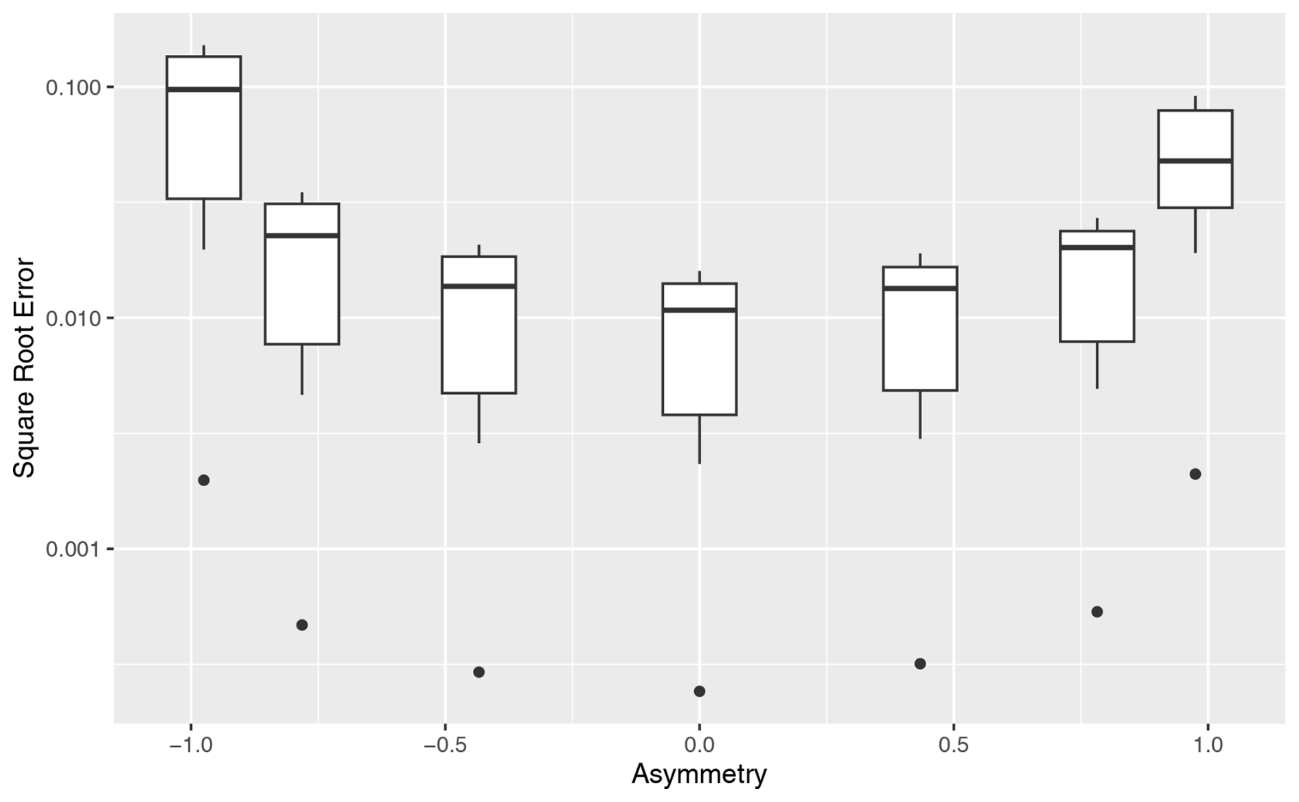
Figure 16 Boxplot of DISORT error as a function of asymmetry. Data is for the run with nn=168. Strong asymmetry increases error.

Figure 17 Squared error over test set for EigenFlux vs. DISORT, plotted on a log-log scale.

The change in accuracy for EigenFlux across the test cases is largely a function of the scatter fraction- the lower the absorption, the lower the accuracy as in Fig. 13. Figure 14 shows that there is a weak tendency for the method to be more accurate at the extreme points of asymmetry. The change in accuracy for DISORT across the test cases is similar in behavior to EigenFlux as a function of the scatter fraction- the lower the absorption, the lower the accuracy as in Fig. 15. However unlike EigenFlux, Fig. 16 shows DISORT is less accurate at the extreme points of asymmetry. The same input parameters were used to directly compare the EigenFlux and DISORT results and timing. The Henyey-Greenstein phase function was used for these comparisons.

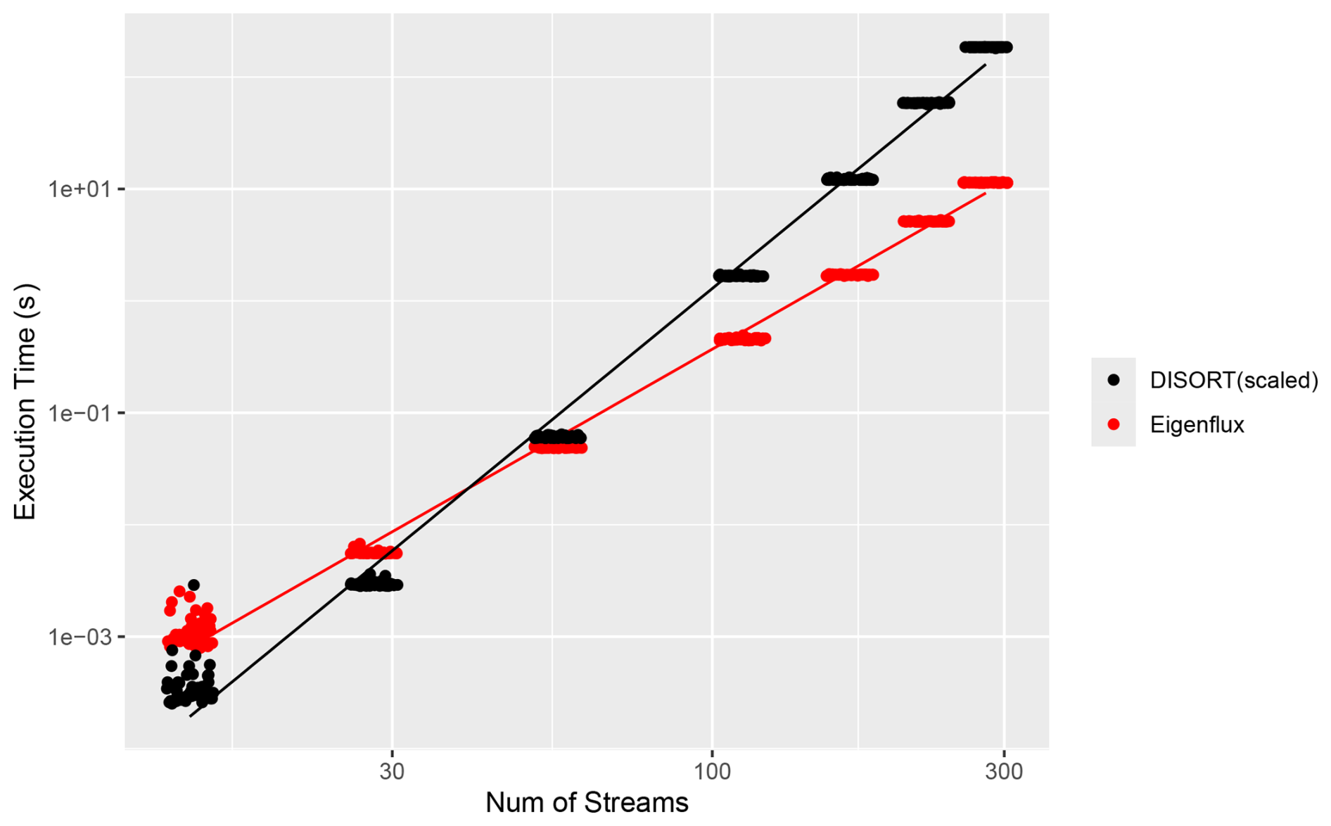
Figure 18 Execution time for EigenFlux vs. DISORT, plotted on a log-log scale. DISORT times have been scaled by number of source beams since EigenFlux always computes multiple source beams.

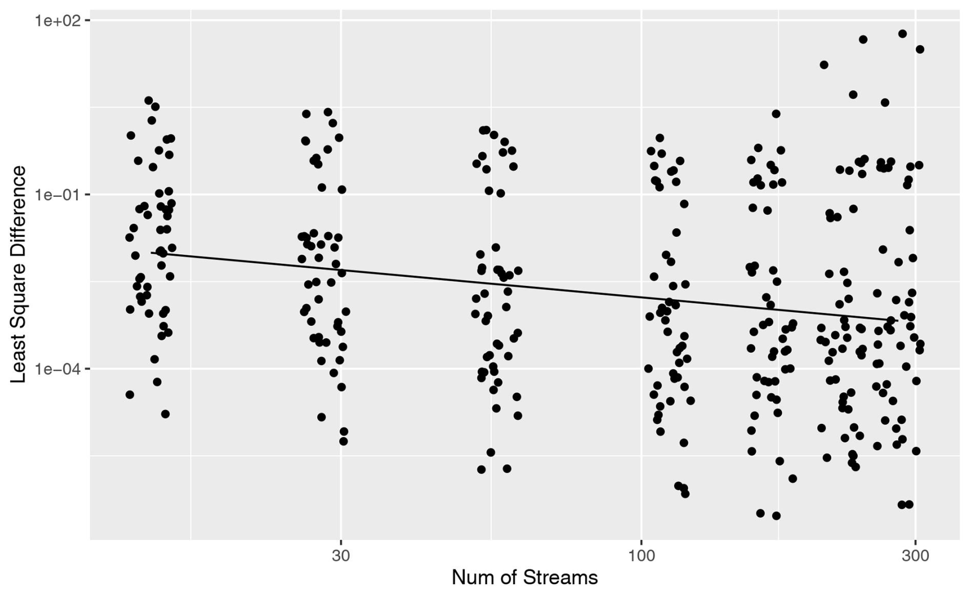
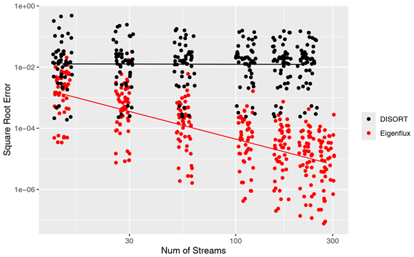
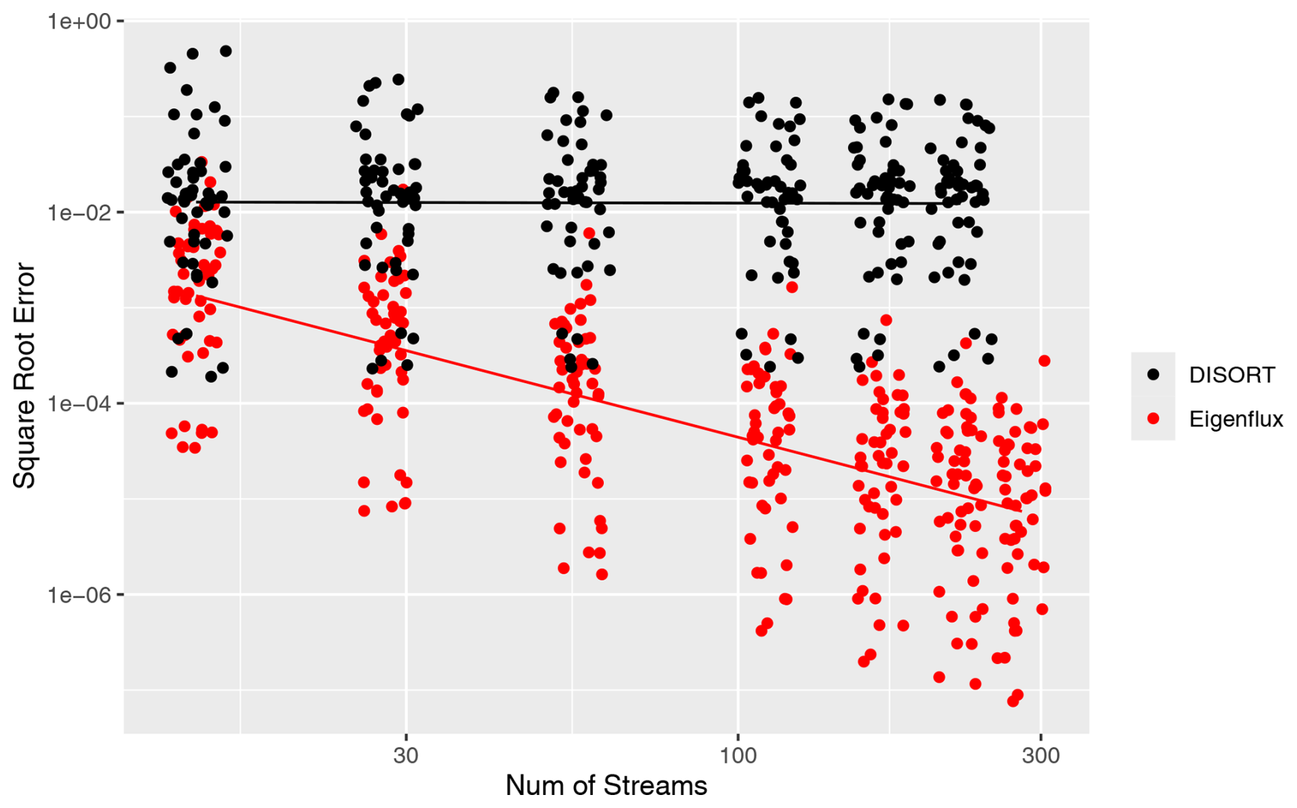
Figure 19 Least square difference between intensities computed by EigenFlux vs. DISORT, plotted on a log-log scale. Jitter added to number of streams to expand point cloud.

One issue in the comparison is that EigenFlux always computes across a spanning set of source functions, whereas DISORT computes a single source function at a time. As a result, the DISORT times in Fig. 18 were scaled to correspond to the EigenFlux usage. The result shows that DISORT is faster for lower numbers of streams, whereas EignFlux is faster for higher numbers of streams, with a crossover at n=56.

The difference between the intensities computed by EigenFlux versus DISORT show considerable variance, as seen in Fig. 19. Figures 21 and 20 show that this is largely a factor of the asymmetry- DISORT's solution deteriorates for strongly scattering problems.

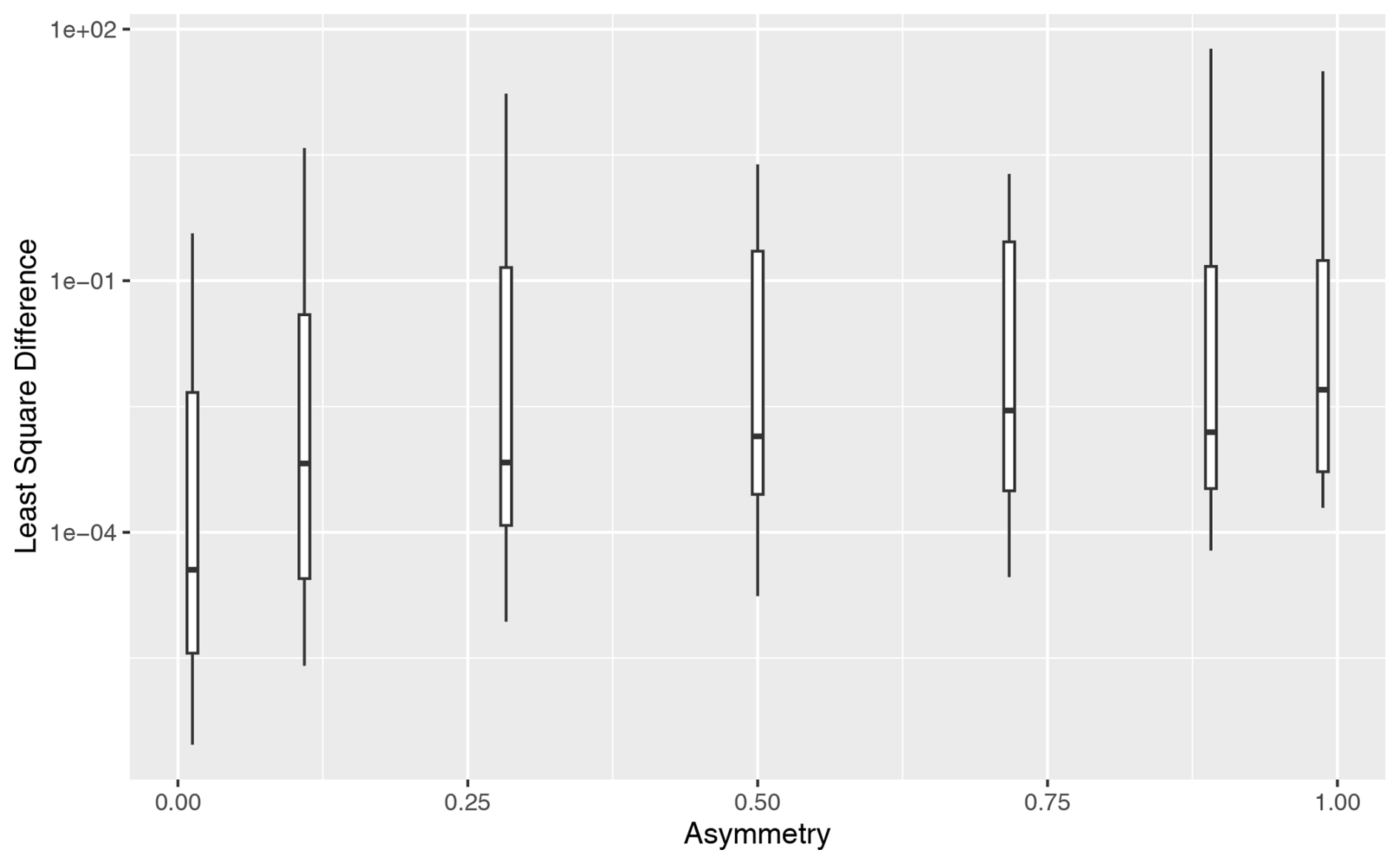
Figure 20 Least square difference between EigenFlux and DISORT as a function of scattering fraction, plotted on a log scale. Lower absorption increases the difference, very slightly.

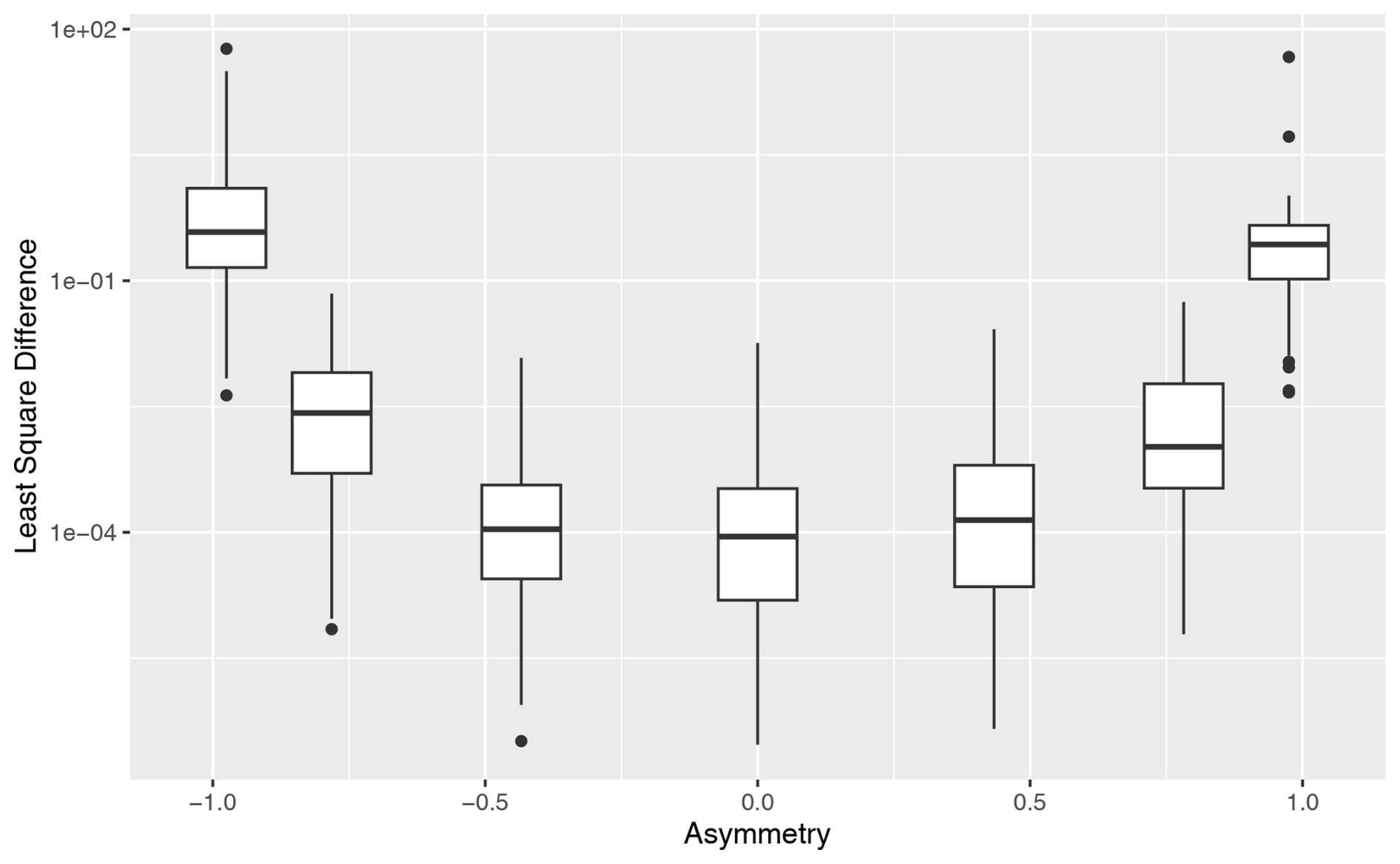
Figure 21 Least square difference between EigenFlux and DISORT as a function of asymmetry, plotted on a log scale. Strong asymmetry increases the difference.

4 Conclusions

EigenFlux is a novel approach to solving the radiative transfer problem, using a natural reflectance structure and a Galerkin mesh approximation scheme that allows for flexible calculation points including linear and Chebyshev point distributions, which in turn allows for accurate reduced order approximations of phase functions which are strongly forward scattering or have significant backward scattering components. The resulting implementation shows strong numerical accuracy and favorable computational scaling in comparison with DISORT across the test cases investigated here. The primary novelty of EigenFlux lies in its combination of natural-reflectance stabilization, localized mesh approximations, and eigenmode decomposition, allowing stable treatment of highly asymmetric scattering regimes that are difficult for conventional discrete-ordinate methods.

Figure 14 shows that EigenFlux is more accurate for extreme scattering points while Fig. 21 shows that the comparable DISORT code is less accurate for the same extreme points. Figure 17 shows that EigenFlux is is more and more accurate that DISORT as the number of streams increases, with an accuracy increase by a factor of 0.0013 at 168 streams. Figure 18 shows that EigenFlux is faster than DISORT for larger numbers of streams, with an even breakpoint at about 56 streams. Analytically, EigenFlux provides insights into the nature of RTM intensity structures. The max eigenvalue determines the limiting distribution of the intensity, and dictates the degree to which the diffuse intensity overcomes (or fails to overcome) the direct intensity as depths increase. In a low-absorption system such as snow and ice, the diffuse intensity quickly overcomes the direct intensity. The analysis here also shows that for low absorbance systems such as snow and ice, the use of two-stream approximation as an inverse model to infer the asymmetry and single stage albedo from measured transmission and reflectance can be problematic as multiple values for the asymmetry and single stage albedo can result in identical transmission and reflectance measures.

The present implementation of EigenFlux is limited to scalar radiative transfer in plane-parallel geometries and does not currently include polarization, thermal emission, or fully spherical atmospheric effects. Inhomogeneous systems are represented through combinations of homogeneous layers rather than through fully continuous spatial variation. These limitations define important directions for future development. Future work could include extension to pseudo-spherical geometries, inclusion of polarization and thermal emission, adaptive mesh refinement, and optimization for specific architectures. The flexible mesh and eigenmode structure of EigenFlux may also prove useful for inverse retrieval applications and coupling to atmospheric, oceanographic, and graphics-rendering systems.