New operational perspective to identify aerosols and hydrometeors in real-time with a pioneering algorithm (CONIOPOL) based on single-wavelength polarization lidar (CL61)

Air quality monitoring and climate studies require continuous, vertically resolved observations to characterize aerosols and their impact on radiation, cloud microphysics, and atmospheric composition. In this study, we present CONIOPOL (CONIOlogy + POLarization), an automated depolarization-based classification algorithm developed with the polarized Automatic Lidar Ceilometer (ALC), CL61 (Vaisala Oyj, Finland). The algorithm combines volume linear depolarization ratio (VDR), attenuated backscatter (ATB), and cloud-base height (CBH) retrievals to distinguish between aerosols, cloud phase, and precipitation, and to further classify aerosol subtypes.

One full year (February 2024–January 2025) of observations collected at Uccle (Belgium) was analyzed to investigate the seasonal and vertical distributions of the identified atmospheric targets. Aerosol classifications were assessed through a conditional comparison, using Copernicus Atmosphere Monitoring Service (CAMS) Global Forecast products. CONIOPOL successfully identified dust, smoke/marine, continental, and mixed aerosol environments showing strong temporal and vertical correspondence with CAMS, in particular for transported mineral dust and smoke plumes.

Despite its spectral limitations, the single-wavelength polarization-enabled ALC allows continuous, high-resolution aerosol classification over extended periods, providing a consistent observational dataset for investigating the seasonal evolution of aerosol types over mid-latitude Europe. These findings underscore the potential of polarization-enabled ALCs for long-term aerosol climatology and air quality monitoring, bridging temporal gaps between satellite, in situ, and multi-wavelength lidar observations.

1 Introduction

Aerosols and clouds are key components of the Earth's atmosphere, exerting a major influence on climate, air quality, and weather systems through their interactions with radiation and cloud microphysics (Illingworth et al., 2015; IPCC, 2023). They modulate the Earth's radiative balance by scattering and absorbing solar and terrestrial radiation and by acting as cloud condensation and ice-nucleating particles. Understanding their vertical distribution, composition, and evolution is therefore essential for constraining radiative forcing estimates and improving both weather and climate models.

In recent years, Europe has experienced an increased recurrence of transcontinental aerosol events, notably Saharan dust intrusions carried thousands of kilometers northward (Cuevas-Agulló et al., 2024; Monteiro et al., 2022; Vogel et al., 2025), and long-range smoke plumes from intense wildfires in North America, in particular Canada (Baars et al., 2021; Hu et al., 2019; Markowicz et al., 2016; Masoom et al., 2026; Sicard et al., 2019). These episodes can substantially modify the atmospheric radiative budget, degrade air quality, and influence cloud properties far from their source regions (Haywood and Boucher, 2000). Characterizing and monitoring such events require continuous, vertically resolved observations capable of discriminating between aerosol types and quantifying their optical and microphysical properties (Pappalardo et al., 2014).

Aerosol vertical profiles can be obtained using a range of observational methods. In situ measurements from aircraft (e.g. Jurányi et al., 2025), balloon-borne (e.g. Ravi Kiran et al., 2022), hot-air balloons (e.g. Petäjä et al., 2012), zeppelins (e.g. Tillmann et al., 2022), towers (e.g. Franco et al., 2024), or unmanned aerial vehicles (e.g. Brus et al., 2021) provide detailed chemical and microphysical characterizations but are limited in temporal and spatial coverage. In contrast, active remote sensing with lidar systems within the ACTRIS framework enables continuous retrievals of aerosol optical properties, allowing high-resolution monitoring of the vertical structure of aerosols and clouds (Laj et al., 2024).

Depolarization is one of the most powerful lidar observables for differentiating aerosol and cloud types. It quantifies changes in the polarization state of backscattered light induced by atmospheric scatterers. The quantity directly measured by a polarization lidar is the volume linear depolarization ratio (VDR), defined as the ratio of the cross-polarized (XPOL) to co-polarized (PPOL) backscattered signal and containing contributions from both atmospheric molecules and particles. By removing the molecular contribution, one obtains the particulate linear depolarization ratio (PDR), which characterizes the depolarization properties of aerosols and cloud particles alone. Depolarization mainly arises from light scattering by non-spherical particles such as mineral dust, volcanic ash, or ice crystals (Freudenthaler et al., 2009), which modify the polarization state of the incident light. Spherical particles, in contrast, preserve the incident polarization, producing low depolarization ratios. Depolarization thus provides a robust means of classifying atmospheric particles into depolarizing (e.g., dust, ice) and non-depolarizing (e.g., smoke, sulfate) types. Depolarization measurements also enable cloud-phase identification, distinguishing liquid-phase clouds composed of nearly spherical droplets from ice-phase clouds containing non-spherical crystals (Lewis et al., 2020; Neely et al., 2013).

Satellite observations based on depolarization are essential in this context, as they provide global, continuous, and synoptic coverage, capturing long-range transport events that ground-based instruments alone cannot resolve. Instruments such as CALIOP (Cloud-Aerosol Lidar with Orthogonal Polarization, Winker et al., 2009) aboard CALIPSO measure PDR in the vertical column, allowing discrimination between spherical and non-spherical particles. Similarly, depolarization-capable spaceborne lidars such as ATLID onboard ESA's EarthCARE mission (Illingworth et al., 2015; Wehr et al., 2023) exploit depolarization to identify aerosol types and cloud phases with high vertical resolution. By providing repeated, large-scale measurements, satellite depolarization observations are crucial for detecting and tracking transcontinental aerosol transport events – such as Saharan dust or North American smoke plumes – and for validating global and regional aerosol transport models.

Airborne lidar systems further complement spaceborne observations by offering flexible, high-resolution measurements over targeted regions. Instruments such as NASA's High Spectral Resolution Lidar (HSRL; Burton et al., 2018; Hair et al., 2008) and the French LNG lidar aboard the SAFIRE Falcon 20 (Chazette et al., 2019) can accurately profile aerosol and cloud optical properties with fine vertical and horizontal resolution, bridging the scale gap between satellite and ground-based measurements.

Complementary to these spaceborne and airborne systems, ground-based lidar networks, including multi-wavelength lidar and single-wavelength Automatic Lidar Ceilometer (ALC) systems, provide continuous, high-temporal-resolution observations of the vertical structure of aerosols and clouds (Illingworth et al., 2019) usually covering the whole troposphere. Multi-wavelength lidars represent the most advanced class of ground-based systems, as they combine measurements at several laser wavelengths and polarization states. This synergy allows for a more comprehensive retrieval of aerosol optical and microphysical properties, including particle size distribution, refractive index, and complex mixtures (Müller et al., 2007). In contrast, single-wavelength systems such as ALCs offer robust and continuous profiling but remain limited in their capability to characterize particle size and composition (Madonna et al., 2015, 2018; Wiegner et al., 2014).

Recent technological developments have led to the commercial availability of compact ALCs equipped with depolarization channels, enabling unattended, routine monitoring of particle shape and cloud phase at a fraction of the cost of multi-wavelength lidars. Among commercially available instruments, only two currently integrate depolarization capability with single wavelength: the Vaisala CL61 and the Halo Photonics StreamLine Doppler wind lidar. Both have been validated in numerous studies demonstrating their accuracy and suitability for operational applications. The Vaisala CL61 has been employed for a wide range of aerosol and cloud studies (Bedoya-Velásquez et al., 2022; Chen et al., 2025; Filioglou et al., 2023, 2025; Inoue et al., 2025; Inoue and Sato, 2023; Karle et al., 2025; Looschelders et al., 2025; Tukiainen et al., 2025), while the Halo Photonics StreamLine has been used to investigate aerosol–cloud interactions and to validate depolarization retrievals (Bohlmann et al., 2021; Le et al., 2024; Vakkari et al., 2021).

Recent studies have developed increasingly sophisticated frameworks for aerosol classification based on the PDR and complementary optical parameters. Multi-wavelength lidar observations have shown that combining PDR, attenuated backscatter (ATB), and lidar ratio enables reliable discrimination among major aerosol types, including dust, smoke, and marine particles (Baars et al., 2017; Burton et al., 2012; Groß et al., 2013). However, similar classifications can also be achieved with single-wavelength systems when rigorously calibrated against reference instruments, as demonstrated by Papetta et al. (2024), and by the successful use of the single-wavelength ATLID instrument (Wehr et al., 2023). This highlights that, while multi-wavelength lidars provide more detailed insights into aerosol microphysics, properly calibrated single-wavelength systems can still deliver valuable classification capabilities.

Depolarization-based aerosol classification typically follows a stepwise, decision-tree approach. Lidar signals are first calibrated to retrieve PDR and ATB profiles, after which PDR thresholds distinguish spherical from non-spherical particles. Auxiliary parameters such as lidar ratio, backscatter coefficient, and Ångström exponent further refine the classification, including the identification of mixed or layered aerosols. Additional temporal and vertical averaging, along with quality screening, helps reduce uncertainties related to noise and layer overlap. This modular framework allows ground-based polarization lidars to produce continuous, high-resolution aerosol and cloud typing for both climatological and operational applications.

In parallel, machine learning (ML) methods have become powerful tools for lidar-based aerosol classification. Supervised algorithms such as Random Forests and Support Vector Machines trained on labeled datasets can capture nonlinear relationships among lidar-derived variables, improving classification accuracy under diverse conditions (del Águila et al., 2025; Farhani et al., 2021; Nicolae et al., 2018). More recently, deep learning (DL) architectures, particularly Convolutional Neural Networks (CNNs), have shown strong potential for identifying complex aerosol features directly from vertical profiles. CNNs can extract spatial patterns within lidar signals, enabling finer discrimination of mixed or overlapping aerosol layers (Lolli, 2023). These advances indicate a growing trend toward hybrid frameworks that combine physical constraints with ML-based feature extraction, aiming to leverage the strengths of both physics-driven and data-driven approaches for improved aerosol and cloud classification.

Despite these advances, no operational classification framework specifically designed for continuous observations from commercially available single-wavelength polarization ceilometers has yet been comprehensively described and evaluated over a full annual cycle. However, aerosol classification using single-wavelength depolarization measurements remains particularly challenging, as it requires careful calibration and robust algorithms to separate aerosol types and cloud phases under varying atmospheric conditions. To address this gap, the CONIOPOL algorithm was developed at the Royal Meteorological Institute of Belgium to automatically classify atmospheric targets detected by the CL61 at the Uccle site in Brussels, Belgium. The algorithm combines depolarization, ATB, and cloud-base height (CBH) data to distinguish between aerosols, clouds, and precipitation and to further categorize aerosol types. By integrating filtering, smoothing, threshold-based classification, and clustering methods, CONIOPOL enables continuous, high-resolution monitoring of aerosol–cloud interactions and their seasonal variability.

The present study has four main objectives:

• To describe and implement the CONIOPOL algorithm for depolarization-based classification using the Vaisala CL61.

• To evaluate the performance and stability of the instrument calibration and algorithm thresholds at the Uccle site over an annual cycle.

• To characterize the occurrence, seasonal variability, and vertical distribution of the different aerosol and hydrometeor categories identified by CONIOPOL.

• To assess the physical consistency of the CONIOPOL aerosol classifications through a conditional comparison with Copernicus Atmosphere Monitoring Service (CAMS) Global Forecast aerosol fields.

Uccle provides an ideal testbed for this study, owing to its long-term atmospheric observation record and its location in a temperate oceanic environment, influenced by both natural and anthropogenic aerosol sources. The synergy between continuous high-resolution ALC observations and atmospheric composition modelling provides complementary information on aerosol occurrence and transport. While CONIOPOL resolves the temporal variability and fine-scale vertical structure of aerosol layers, CAMS provides the large-scale atmospheric context. Together, these datasets contribute to the development and evaluation of automated aerosol classification systems for operational monitoring within European observation networks.

2 Site description

The Uccle site is located in the southern part of Brussels (50.8° N, 4.35° E) in Belgium at approximately 100 m above sea level. Established in 1886, it is one of the longest-running atmospheric monitoring stations in Europe and is a member of many international networks such as the World Meteorological Organization's Global Atmosphere Watch (GAW), the Network for the Detection of Atmospheric Composition Change (NDACC), and in near future in the Aerosols, Clouds, and Trace Gases Research Infrastructure (ACTRIS). The site is situated within a suburban environment, including residential neighborhoods, parks, and green spaces, minimizing local pollution influences and ensuring that measurements are representative of regional atmospheric conditions.

Uccle experiences a temperate oceanic climate (Köppen classification: Cfb) and prevailing westerly winds associated with the North Atlantic which strongly favor the transport of aerosols from both regional and long-range sources. Westerly and southwesterly winds can carry mineral dust from the Sahara and southern Europe, sea salt from the North Sea, smoke from wildfires in southern Europe or even Canada during extreme wildfire seasons, depending on the synoptic conditions. Local and regional anthropogenic aerosols, including urban and industrial emissions, also contribute to the observed aerosol load, while natural sources such as biogenic aerosols play an additional role (Flemish Environment Agency, 2020; IRCELINE, 2023). These include primary biological particles (e.g., pollen, spores) as well as secondary organic aerosols formed from the oxidation of biogenic volatile organic compounds (BVOCs), particularly during the growing season. Seasonal variations in wind patterns, precipitation, and boundary-layer dynamics further control aerosol dispersion, mixing, and removal.

3 Vaisala CL61 ALC

At Uccle, a single ALC (CL61, Vaisala Oyj, Finland) is installed. The instrument is operated in a fixed zenith-pointing mode, providing continuous vertical profiling of the atmospheric column above the measurement site. It is specifically designed for atmospheric profiling and provides advanced capabilities for cloud and aerosol detection (Roininen et al., 2025). Using a 910.55 nm InGaAs diode laser, the CL61 measures ATB volume profiles with a vertical resolution of 4.8 m over a range from 0 to 15.4 km. A key feature distinguishing the CL61 from other ALCs is its depolarization measurement capability, which enables the differentiation between solid, liquid, and mixed-phase cloud and precipitation particles. The degree of depolarization is influenced by both aerosols and air molecules and is expressed as the volume linear depolarization ratio (VDR), defined as the ratio of the cross-polarized (XPOL) to the parallel-polarized (PPOL) signal components. The CL61 alternates acquisition of XPOL and PPOL signals with an integration time of 0.2 s for each, and complete profiles are averaged over 5 s prior to analysis. The minimum averaging interval is 5 s for ATB and 10 s for depolarization. In this study, a 30 s averaging interval is applied to both. This configuration enables detailed vertical profiling of the atmosphere, including the detection of CBH (determined internally at a 5 s resolution, independent of user-defined averaging, based on data collected during the last 30 min), aerosol layers, and boundary layer structures. The manufacturer provides an instrument-specific overlap function, expressed as a percentage from 0 % to 100 %, which characterizes the region of incomplete optical overlap, also known as the blind zone. Wagner et al. (2024) recommend discarding observations in the blind zone, which they define as being from the height the overlap function reaches 3 % down to the sensor. For the CL61 employed in this study, this height deduced from the specific overlap function of the instrument corresponds to 33.6 m. However, in accordance with the recommendations of Le et al. (2026) and Looschelders et al. (2025), measurements below 50 m are excluded from the analysis to ensure the reliability of the retrieved atmospheric properties.

The instrument operates autonomously under all weather conditions and requires only minimal maintenance, primarily the regular cleaning of the optical window, which is essential for preserving data quality. Measurement data and internal monitoring parameters are provided every 5 min in NetCDF format, ensuring interoperability with a wide range of reading tools. In this study, the measurement period considered spans from 13 February 2024 (instrument start-up) to 30 January 2025.

4 Algorithm design

The CONIOPOL algorithm uses range, ATB, VDR, and CL61-derived CBH to classify aerosol types, cloud phases, and precipitation types. The processing chain begins with signal conditioning and quality control, including SNR-based filtering and spatiotemporal smoothing, followed by empirically defined thresholds for aerosol, cloud, and precipitation classification.

4.1 Calibration

Accurate calibration of both ATB profiles and depolarization is essential for the reliable performance of CONIOPOL in automatic target classification. The ATB data provided by the CL61 are calibrated against a reference instrument that was calibrated at factory (Wagner et al., 2024) using the cloud calibration method proposed by O'Connor et al. (2004), which relies on the well-characterized and stable optical properties of liquid water clouds. While the calibration constant can be updated, its stability should be verified through monthly monitoring to identify potential drifts from the factory setting and to ensure the long-term consistency of the ATB measurements. In our case, the CL61 calibration remained stable throughout the analysis period.

Unlike more advanced lidars, the CL61 does not incorporate an internal calibrator for the depolarization channel, nor does it allow the user to modify the optical path to include one or to assess the depolarization effect of individual components. In the CL61, depolarization is measured using two filters positioned in front of a single avalanche photodiode detector on the coaxial optical path. Since the same receiver module is used for both PPOL and XPOL signals, no receiver sensitivity calibration is required.

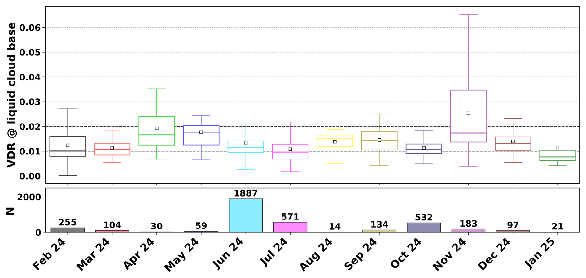
Figure 1 Boxplots of the linear depolarization ratio (VDR) recorded at the cloud base for each month after data filtering at Uccle between February 2024 and January 2025. The horizontal line within each box indicates the median, the square marker denotes the mean, the lower and upper bounds of each box correspond to the 25th and 75th percentiles, and the whiskers extend to the 5th and 95th percentiles. The lower panel displays the number of observations (N) contributing to each monthly boxplot.

Although the polarizer performance in this configuration is expected to remain stable, following the recommendations and methodology of Vakkari et al. (2021) for the Halo StreamLine lidar, we advise monitoring its performance monthly at the base of liquid water clouds. Cloud bases were selected according to this category when the VDR was below 0.1, the retrieved CBH from the CL61 product ranged between 1000 and 4000 m, and the standard deviation of the CBH remained below 15 m over a 10 min interval. While spherical droplets do not inherently polarize the ATB signal, the measured depolarization ratio is not exactly zero due to the non-simultaneous acquisition of PPOL and XPOL signals. This ratio exhibits a slight deviation from zero, reflecting temporal variations in the physical properties of the target between the two measurements. Moreover, Vakkari et al. (2021) reported a slight increase in the PDR within liquid clouds, which was attributed to multiple scattering. To further reduce its potential influence on the PDR, only the first range gates at the cloud base, in the absence of drizzle or precipitation, are used for calibration monitoring. To minimize the influence of drizzle and precipitation, the peak sharpness filter of Hopkin et al. (2019) was applied, and only the first four unsmoothed range gates (57.6–72.0 m) below the retrieved cloud base were retained, provided that the ATB remained greater than 3 × 10⁻⁶ ${\mathrm{m}}^{-\mathrm{1}}{\mathrm{sr}}^{-\mathrm{1}}$ across all selected gates. Data points were selected slightly below the retrieved CBH because Vaisala ALCs typically report the CBH slightly above the altitude of maximum ATB (Wagner et al., 2024). In Fig. 1, the VDR at the base of liquid clouds for each month exhibits no significant drift, with median values generally ranging from 0.01 to 0.02, in agreement with the values of Vakkari et al. (2021) and Le et al. (2024). During the coldest months, some variability may also arise from mixed-phase clouds that were mistakenly considered as liquid-only (Le et al., 2024), which may partly explain the larger spread observed in November.

4.2 SNR filtering and smoothing

In the CONIOPOL algorithm, only the portion of the ATB profile exhibiting a sufficiently high signal-to-noise ratio (SNR) is considered. The noise level is then estimated for each profile of 30 s in an altitude range where no aerosols or clouds are expected, using the SNR preprocessing method of Morille et al. (2007) with a threshold set at 3. Noise calculations are performed on the non-range-corrected ATB within the range gates spanning 14 760 to 15 720 m. The corresponding SNR mask derived from the ATB is subsequently applied identically to the XPOL and PPOL profiles. To suppress isolated noisy pixels while limiting the smoothing of atmospheric gradients and layer boundaries, a two-dimensional median filter with a kernel size of 10 × 10 samples is then applied separately to XPOL and PPOL signals. The filtered ATB and VDR used for the subsequent classification are then derived from the filtered polarized components. Given the CL61 temporal and vertical sampling intervals (30 s and 4.8 m, respectively), this corresponds to a neighborhood of approximately 5 min in time and 48 m in the vertical dimension. The median-filtered signals are subsequently smoothed using a two-dimensional Gaussian filter with standard deviations of (0.3, 0.3) samples in time and range. This light Gaussian smoothing reduces residual high-frequency fluctuations introduced by the median filtering while limiting additional smoothing of atmospheric structures.

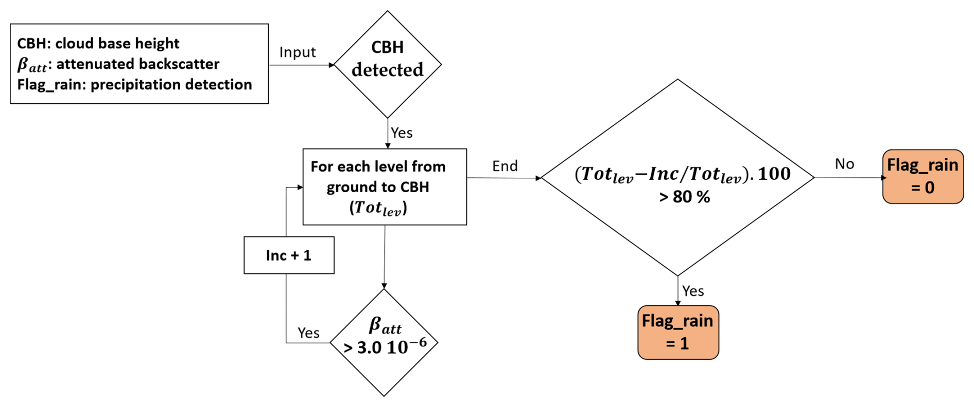
Figure 2 Decision tree employed in CONIOPOL for the detection of precipitation events. The flowchart illustrates the logical sequence of conditions applied to the ATB profiles from the CL61 ALC.

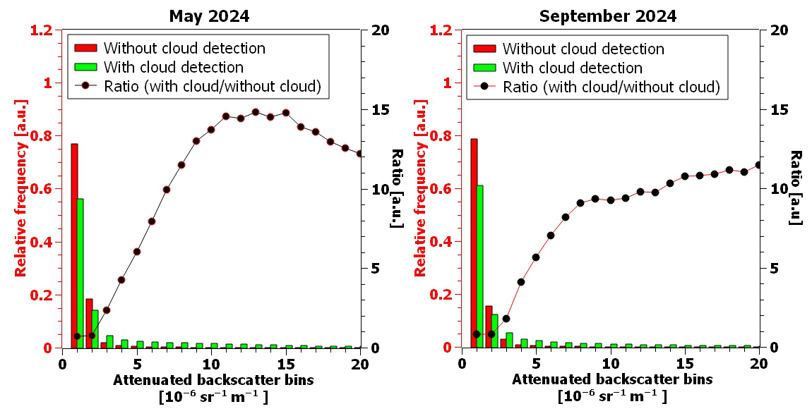
Figure 3 Relative frequency distributions (left y axis) of ATB values with (green) and without (red) cloud detection for May 2024 (left) and September 2024 (right). The black dots represent the ratio of distributions with and without clouds (right y axis). The threshold for distinguishing clouds from clear-sky conditions corresponds to the point where this ratio exceeds 1.

4.3 Threshold-based classification and evaluation

Classification of atmospheric targets as aerosols or clouds/precipitation is based on a threshold applied to the ATB signal. A signal is identified as precipitation when the threshold is exceeded throughout more than 80 % of the vertical range between the ground and the CBH retrieved by the CL61. The flowchart illustrating CONIOPOL's precipitation detection process is shown in Fig. 2.

The threshold for distinguishing aerosols from clouds and precipitation is determined empirically from the relative frequency distributions of ATB values conditioned on the presence or absence of a CBH retrieval from CL61 product. Relative frequency distributions are constructed for both regimes, and the separation threshold is defined where their ratio exceeds unity. This provides a statistically based criterion independent of the CONIOPOL processing chain, which uses CBH as an external input. Figure 3 shows these relative frequency distributions and their corresponding ratios for the months of May and September.

Higher ATB values occur more frequently in the presence of clouds or precipitation, whereas lower values are generally associated with clear-sky conditions. At Uccle, one year of data yielded a threshold of 3 × 10⁻⁶ ${\mathrm{sr}}^{-\mathrm{1}}{\mathrm{m}}^{-\mathrm{1}}$, which was consistent across months as illustrated partially in Fig. 3, and aligns with the value reported by Van Tricht et al. (2014) for distinguishing clear and cloudy conditions using ALCs (CT25K and CL31) operating at a wavelength similar to the CL61. This threshold is lower than 10⁻⁵ ${\mathrm{sr}}^{-\mathrm{1}}{\mathrm{m}}^{-\mathrm{1}}$ reported by Manninen et al. (2018) and 5 × 10⁻⁵ ${\mathrm{sr}}^{-\mathrm{1}}{\mathrm{m}}^{-\mathrm{1}}$ used by Harvey et al. (2013) for cloud detection with the Halo Photonics Streamline Scanning Doppler Lidar.

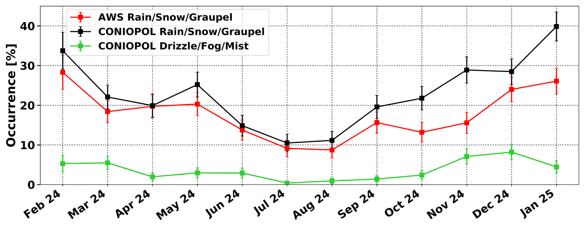
Figure 4 Monthly occurrence of surface precipitation events from February 2024 to January 2025 derived from CONIOPOL and measured by the automatic weather station (AWS) at the Uccle site. The blue curve represents the occurrence of precipitation (rain, wet snow, snow, and graupel reaching the surface) identified by CONIOPOL, while the orange curve shows the corresponding occurrence measured by the AWS weighing rain gauge at a 1 h temporal resolution. The green curve represents the occurrence of drizzle, fog, and mist detected by CONIOPOL. Error bars denote the 95 % confidence intervals.

Applying this threshold to other CL61 instruments within CONIOPOL requires accurate calibration of the ATB signal and regular maintenance of the instrument window. Furthermore, as a fixed ATB threshold is used, its applicability may be affected by exceptionally strong aerosol backscatter, particularly in dense plumes close to emission sources.

The validity of precipitation detection using this threshold was assessed by comparing the monthly precipitation (rain, snow, wet snow, and graupel reaching the surface) occurrences derived from CONIOPOL with those recorded by a rain gauge (OTT Pluvio1, OTT Hydromet) installed near the CL61 (Fig. 4) in Uccle. The occurrence of precipitation detection by CONIOPOL is generally 5 %–13 % higher than that derived from the rain gauge when using a 1 h temporal resolution. This positive bias is statistically significant during the autumn and winter seasons. A plausible contribution to this positive bias is the higher frequency of fog, mist, and drizzle-like conditions during these periods, for which discrimination from precipitation remains challenging. As further discussed in the sensitivity analysis (Sect. 4.7), measurement variability in VDR may additionally cause observations close to hydrometeor classification thresholds to shift between neighbouring categories. To enhance discrimination between precipitation/drizzle and fog/mist, it is recommended to combine the ALC with an additional ground-based remote sensing instrument, such as a Doppler radar (Acquistapace et al., 2019; O'Connor et al., 2005) or a Doppler wind lidar with a depolarization channel such as the Halo Photonics Streamline (Le et al., 2024).

4.4 Depolarization ratio

After separating aerosols, clouds, and precipitation, the identification of aerosols can be further refined using the depolarization ratio, which provides essential, although not comprehensive, quantitative information for aerosol classification (Comerón et al., 2017). High PDR values (greater than 0.2) are typically associated with non-spherical particles such as volcanic ash or mineral dust (Groß et al., 2012). In contrast, values close to 0 indicate spherical particles, such as marine aerosols, while intermediate values reflect mixtures of spherical and non-spherical particles.

Although PDR is a powerful indicator of particle sphericity, it cannot uniquely identify aerosol type on its own. A more robust classification requires the use of dual-wavelength lidar and polarized channels to retrieve additional optical parameters such as the lidar ratio and the Ångström exponent, which provide complementary information on aerosol size and composition. When using only PDR to classify aerosols, parameters like aerosol size distribution, aspherical aerosol orientation, mixture of aerosol types, and hygroscopic growth effects can impact the PDR and lead to ambiguous identification.

In this study, we use the VDR provided directly by the CL61. The VDR includes contributions from both molecular and particulate backscatter, although the relative contribution of molecular scattering decreases with increasing wavelength and in particle-dominated atmospheric layers due to the strong wavelength dependence of Rayleigh scattering. At 910 nm, in the presence of aerosol layers, the CL61 signal is therefore expected to be primarily driven by particulate scattering, with a reduced contribution from molecular backscatter (Haarig et al., 2025; Vakkari et al., 2021). For reference, the molecular backscatter coefficient at 910 nm is approximately 43 times lower than at 355 nm.

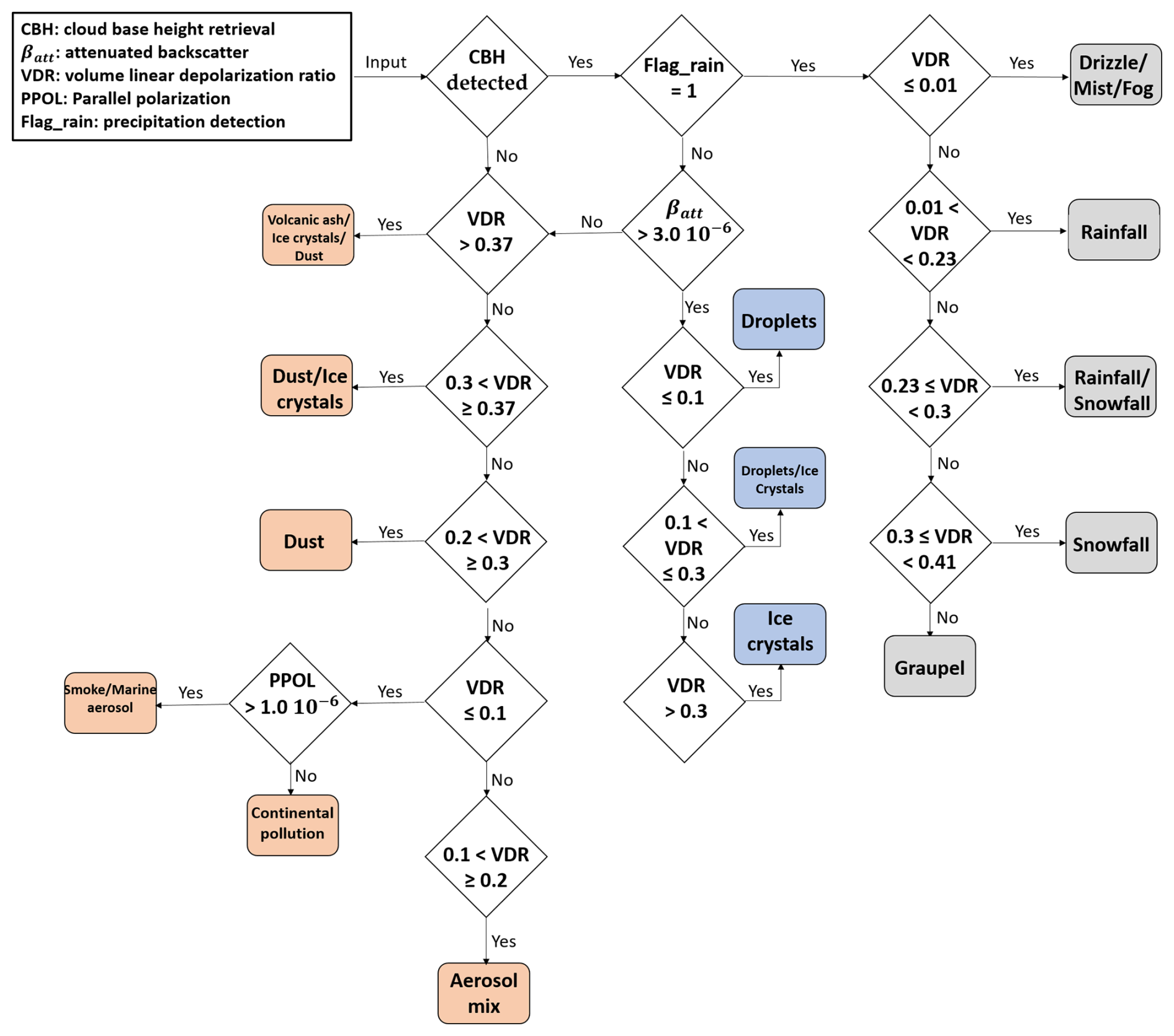
Figure 5 Decision tree for aerosol and cloud phase, and precipitation classification applied in CONIOPOL. The flowchart illustrates the sequence of conditions used to discriminate the different target types based on ALC measurements (ATB, VDR, PPOL) and on the ALC-derived CBH.

Given the limited discriminatory power of VDR alone, methodological choices are required to ensure a consistent aerosol classification while minimizing misclassification arising from overlapping depolarization signatures. Rather than assigning all observations to a limited number of discrete aerosol/cloud phase types, CONIOPOL introduces transitional classes to represent observations sharing characteristics of multiple aerosol, cloud, or precipitation types. This approach provides a more flexible classification framework and better represents the continuous nature of atmospheric particles and hydrometeors. Accordingly, CONIOPOL classifies atmospheric targets using an explicit scheme comprising both primary classes and transitional categories. The overall classification methodology is summarized in the decision tree shown in Fig. 5.

It should also be noted that most aerosol classification schemes reported in the literature have been developed using depolarization measurements at other wavelengths, primarily at the shorter wavelengths of 355 and 532 nm, but also at 1064 nm (Freudenthaler et al., 2009; Haarig et al., 2018). Consequently, the threshold values commonly used to distinguish aerosol types may not be directly transferable to measurements performed at 910 nm. Several studies (Freudenthaler et al., 2009; Haarig et al., 2022; Vakkari et al., 2021) have shown that particle depolarization exhibits spectral dependence, the magnitude and direction of which vary according to aerosol type, particle size, shape, and composition.

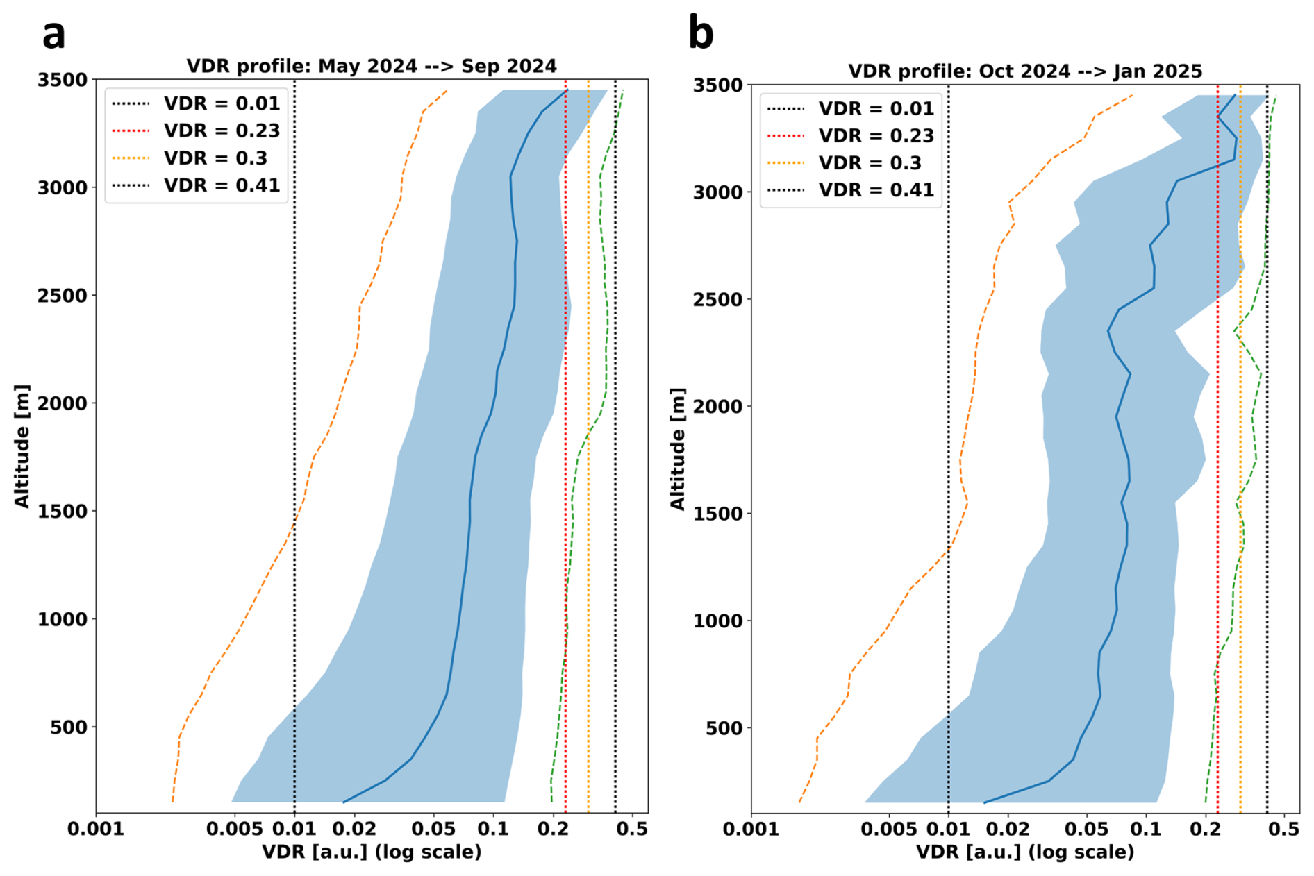
Figure 6 Vertical distribution of VDR measured by the CL61 during precipitation events for the warm season (May–September 2024; a) and cold season (October 2024–January 2025; b). Blue curves indicate the median, shaded areas the interquartile range (25th–75th percentiles), and dashed green curves the 90th percentile (P90), used to derive the precipitation-phase thresholds adopted by CONIOPOL. Vertical dotted lines indicate the four selected VDR thresholds (0.01, 0.23, 0.30, and 0.41) defining the boundaries between the five precipitation categories: fog/drizzle/mist (VDR < 0.01), liquid precipitation (0.01 ≤ VDR < 0.23), mixed-phase precipitation (0.23 ≤ VDR < 0.30), snow (0.30 ≤ VDR < 0.41), and graupel (VDR ≥ 0.41).

4.4.1 Cloud phase

To define cloud phase classification, we follow the scheme proposed by Wu et al. (2025), which defines a liquid phase for VDR < 0.1, a mixed liquid–solid transition phase for 0.1 ≤ VDR ≤ 0.3, and a solid (ice crystal) phase for VDR > 0.3. It should be noted, however, that preferentially horizontally oriented ice crystals may exhibit substantially reduced VDR when observed by a zenith-pointing lidar (Noel and Sassen, 2005). Such orientations are typically observed in weakly turbulent ice clouds composed of planar crystals, whereas turbulent conditions generally randomize crystal orientations. Consequently, this effect is expected to occur only under specific atmospheric conditions and is therefore unlikely to represent a systematic source of bias in the cloud-phase classification.

4.4.2 Precipitation/Fog

For fog, drizzle, and mist detection, the characteristic VDR observed at the base of liquid-phase clouds was adopted as the threshold (Fig. 1), corresponding to VDR < 0.01. Above this threshold, the presence of larger liquid droplets is assumed. As droplet size increases, deviations from perfect sphericity become more pronounced owing to aerodynamic deformation during their fall (Sassen, 2003), resulting in higher depolarization ratios. Consequently, VDR values exceeding 0.01 are interpreted as liquid precipitation. Nevertheless, as discussed previously, a clear distinction between fog, drizzle, and mist remains challenging because these phenomena form a continuum in droplet size and often occur simultaneously under similar meteorological conditions.

To distinguish between rain and snow, the 90th percentile (P90) of the VDR distribution was analysed during periods identified as rainfall events. The analysis was first performed for the period from May to September 2024, during which no snowfall reaching the surface was reported (Fig. 6a). Under these conditions, liquid precipitation was consistently associated with VDR values ranging from 0.01 to 0.23. At altitudes above approximately 2000 m, however, P90 values increased to between 0.30 and 0.41, indicating the presence of snowflakes aloft despite liquid precipitation being observed at the surface, a situation frequently encountered during summer. Between these two regimes, a transition zone characterized by VDR values between 0.23 and 0.30 was identified, corresponding to mixed-phase precipitation containing both liquid droplets and snowflakes. The same analysis was subsequently applied to the winter period (October 2024 to January 2025) (Fig. 6b). A similar transition zone was observed, although it occurred at lower altitudes and extended over a deeper vertical layer. Above approximately 1500 m, P90 values generally ranged between 0.30 and 0.41, consistent with predominantly solid precipitation. VDR values exceeding 0.41 were attributed to heavily rimed ice particles and aggregates, which were classified as graupel.

4.4.3 Aerosols

To define the dust class, we rely on the observations reported by Freudenthaler et al. (2009), who identified pure dust layers at wavelengths of 710 and 1064 nm and measured particle depolarization ratio (PDR) values ranging from 0.2 to 0.3. These thresholds are adopted here and applied to the VDR measurements provided by the CL61. Similar PDR values (0.20–0.30) were also reported by Burton et al. (2015) during Saharan dust transport events. In contrast, larger PDR values (> 0.30) were observed during dust outbreaks originating from nearby source regions and were attributed to a greater proportion of coarse mineral dust particles, which produce stronger depolarization signals (Burton et al., 2015; Haarig et al., 2022). Comparable observations were reported by Vakkari et al. (2021), who measured PDR values close to 0.30 during mineral dust events at a wavelength of 1565 nm. Based on these previous studies, VDR values between 0.20 and 0.30 were assigned to the dust class in CONIOPOL.

The presence of dust mixed with less depolarizing aerosol types can substantially reduce the observed depolarization ratio, sometimes below 0.2, particularly at shorter wavelengths such as 355 nm (Haarig et al., 2022). To account for this effect and the inherent ambiguity associated with mixed aerosol populations, an intermediate aerosol mix class is defined for VDR values between 0.1 and 0.2. This category may also include pollen particles, although the studies of Cao et al. (2010) and Filioglou et al. (2023) reported PDR values generally exceeding the range defined here. However, these studies were conducted under specific conditions: the former in laboratory chambers and the latter in close proximity to pollen emission sources, where pollen concentrations were particularly high. Filioglou et al. (2023) further showed that at longer wavelengths (910 and 1565 nm), the PDR–pollen concentration relationship exhibits a saturation behaviour for both pine and birch pollen. Prior to reaching this plateau, PDR values at 910 nm remained below 0.2. Similarly, Bohlmann et al. (2021) also demonstrated that PDR values are strongly influenced by pollen (spruce) concentration. For moderate concentrations of spruce pollen, PDR values measured at 1565 nm remained below 0.2, overlapping with the range defined for this class. Nevertheless, the presence of pollen fragments, which were not explicitly considered in that study, may lead to enhanced depolarization and consequently higher PDR values. As a result, pollen-rich aerosol layers may occasionally overlap with other aerosol classes, introducing additional uncertainty into aerosol classification based solely on depolarization measurements. Although pollen can undergo long-range atmospheric transport (e.g. Sofiev et al., 2006), its influence far from major source regions is expected to be more episodic, resulting in occasional rather than systematic classification uncertainty. In applications primarily focused on mineral dust detection, the contribution of pollen on aerosol classification is therefore expected to remain limited.

For VDR values exceeding 0.3, the possible presence of very large dust particles must be considered. However, such high depolarization values may also indicate the presence of ice crystals, especially in situations where cloud-base detection fails or where residual ice-phase hydrometeors are present within the observed layer. Consequently, observations with VDR > 0.3 should be interpreted with caution and in conjunction with the cloud-phase classification described previously.

To define the volcanic ash class, we rely on observations reported by Groß et al. (2012), who measured PDR values of approximately 0.37 at 532 nm within a pure volcanic ash plume originating from the Icelandic Eyjafjallajökull eruption. Similarly, Ansmann et al. (2010) reported PDR values ranging from 0.35 to 0.40 at 532 nm for the same event, while Marenco and Hogan (2011) obtained a mean depolarization value of 0.34 from lidar measurements at 355 nm. More recently, Filioglou et al. (2026) observed PDR values generally exceeding 0.37 during a volcanic ash event at a wavelength of 1565 nm. Based on these observations, VDR values above 0.37 are considered indicative of volcanic ash. Nevertheless, VDR values exceeding this threshold are not uniquely associated with volcanic ash. Large mineral dust particles and ice crystals may produce similarly high depolarization signatures, leading to potential ambiguities in aerosol identification. Consequently, observations classified as volcanic ash should be interpreted in conjunction with cloud-phase information and the broader meteorological context. The optimal application of the algorithm in contexts of volcanic eruptions requires integration of complementary constraints, including geographical source attribution, air mass origin analysis, and, where available, additional optical parameters. Although the studies cited above span wavelengths from 355 to 1565 nm and suggest a relatively weak spectral dependence of ash depolarization, the transfer of threshold values to 910 nm remains subject to uncertainty.

It should also be noted that studies conducted close to volcanic emission sources often report lower and more variable depolarization values. For example, Bedoya-Velásquez et al. (2022), using a CL61 ALC, reported VDR values ranging from 0.2 to 0.3 in volcanic plumes, while Pisani et al. (2012) observed lidar depolarization ratios at 532 nm ranging from 0.16 to 0.45. The immediate proximity to the volcanic source likely complicates the identification of pure ash plumes because of the complex composition of freshly emitted volcanic plumes and their subsequent evolution, including the progressive formation of weakly depolarizing sulfate aerosols. This mixing can substantially reduce the measured depolarization ratio and broaden the range of observed values.

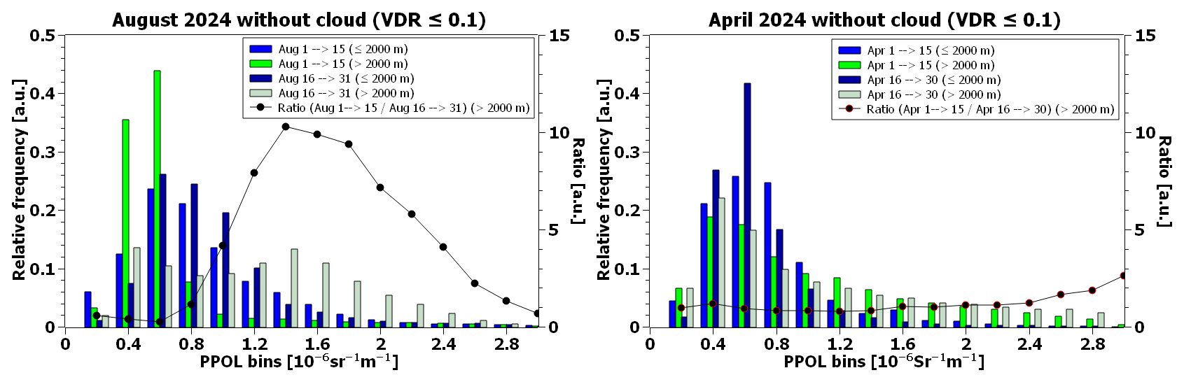
Figure 7 Relative frequency distributions of the parallel-polarized signal (PPOL) for two periods without cloud contamination (VDR ≤ 0.1): (left) August 2024 and (right) April 2024. Colored bars represent distributions for different sub-periods and altitude ranges below and above 2000 m. Specifically, blue denotes the first 15 d of the month below 2000 m, green the first 15 d above 2000 m, grey the last 15 d below 2000 m, and pink the last 15 d above 2000 m. The black points indicate the ratio of the relative frequency between the last 15 d and the first days of the month for altitudes above 2000 m.

The decision to group smoke and marine aerosols into a single classification was motivated by the fact that both aerosol types typically exhibit low PDRs, generally below 0.1 at 532 nm (Groß et al., 2013; Haarig et al., 2017, 2025). While fresh smoke shows little or no wavelength dependence in its PDR, aged smoke exhibits a clear wavelength dependence, with the PDR decreasing with increasing wavelength. However, even for aged smoke, the PDR remains below 0.1 at 1064 nm (Haarig et al., 2018). Both aerosol types are hygroscopic, and their PDR decreases with increasing water vapour content due to hygroscopic growth effects (De Rosa et al., 2025; Haarig et al., 2017).

To discriminate smoke and marine aerosols from continental pollution, a threshold on the PPOL is applied. Unlike continental pollution, which is generally produced by spatially distributed anthropogenic sources and becomes well-mixed within the ABL, smoke originates from localized wildfire sources and is typically transported over long distances in coherent plumes that form well-defined elevated aerosol layers. Depending on the wildfire intensity, the smoke may be injected above the ABL into the free troposphere, where it can be transported over continental to intercontinental scales (Haarig et al., 2018). Marine aerosols, by contrast, are commonly associated with sea-breeze circulations and are generally confined to the lowest atmospheric layers, although the sea-breeze flow may become partially decoupled from the continental ABL (Boyouk et al., 2011). Both smoke and marine aerosols are hygroscopic, and their optical properties are affected by hygroscopic growth. In particular, hygroscopic growth substantially enhances the ATB at 990 nm (Haeffelin et al., 2016), while simultaneously reducing the PDR as particles become more spherical. Consequently, a PPOL threshold alone is not always sufficient to distinguish smoke aerosols from other hygroscopic aerosol types, including marine.

The PPOL threshold, corresponding to a VDR lower than 0.1, was defined based on the ratio between the frequency distribution of PPOL values during a period affected by smoke plume events and the frequency distribution observed during a reference period without smoke plumes. The criterion for threshold selection was that this ratio exceeded unity above 2000 m. For the Uccle site, the ratio was computed using observations from the last 15 d of August 2024 – when the presence of significant smoke plumes was confirmed by CAMS – against the first 15 d of August, serving as the reference period without smoke influence, as illustrated in Fig. 7. The resulting threshold value was set to 1.0 × 10⁻⁶ ${\mathrm{sr}}^{-\mathrm{1}}{\mathrm{m}}^{-\mathrm{1}}$, corresponding to the PPOL value at which the ratio consistently exceeded 1. To ensure that this effect was specifically attributable to smoke and not to background variability, the frequency distribution was also analyzed below 2000 m for both periods, where no substantial differences were observed, confirming that the observed signal enhancement was restricted to altitudes impacted by transported smoke. Furthermore, the robustness of this approach was tested on several control months without smoke intrusions (such as in April 2024). In this case, no significant differences were found between the frequency distributions at the beginning and end of the month, both below and above 2000 m, thereby supporting the methodological validity of the threshold definition. Overall, this procedure strengthens the statistical reliability of the classification framework by minimizing the likelihood of false positives arising from natural variability in the aerosol background.

4.5 Limitations associated with cloud-base detection

The CONIOPOL decision tree uses the cloud-base information provided by the operational Vaisala CL61 algorithm to distinguish between cloud and aerosol branches. Consequently, cloud-base retrieval errors may propagate into the subsequent classification. The Vaisala cloud-base detection algorithm relies primarily on the magnitude of the ATB signal and its vertical gradient. Optically thick liquid clouds are generally detected reliably, whereas optically thin clouds, particularly cirrus, may exhibit weaker ATB gradients and lower signal-to-noise ratios, leading to an overestimation of CBH or, in some cases, to missed detections (Looschelders et al., 2025). Nevertheless, CBH information is only one element of the decision tree, which also relies on ATB, VDR, PPOL intensity, and a two-dimensional sliding-window consistency filter.

When no cloud base is detected, the decision tree deterministically follows the aerosol branch, so optically thin liquid clouds may be classified as smoke/marine aerosol, whereas optically thin ice clouds may be assigned to the dust/ice category. Conversely, dense aerosol layers, such as mineral dust or volcanic ash, may occasionally satisfy the cloud detection criteria of the ALC (Evan et al., 2022), locally activating the cloud branch and producing ice-crystal classifications within parts of the aerosol layer. Adjacent regions, where no cloud base is retrieved, continue to be classified as dust or dust/ice. Cloud-base retrieval errors are therefore expected to produce localized transitions between these categories rather than systematically convert an entire aerosol layer into an ice-cloud detection.

The occurrence statistics presented in this study therefore represent the occurrence of the CONIOPOL classifications rather than a reference cloud climatology. In particular, the reported occurrence of ice crystals reflects both the atmospheric occurrence of ice clouds and the performance of the CBH detection algorithm, particularly for optically thin high-altitude clouds with lower SNR. The analysis of the full measurement ranges up to 15.4 km nevertheless provides a comprehensive characterization of the vertical occurrence of the ice-crystal category. A quantitative assessment of the sensitivity of CONIOPOL to cloud-base retrieval errors would require independent collocated cloud observations, such as cloud radar or Cloudnet products, and is left for future work.

4.6 2D sliding-window consistency filter

A two-dimensional sliding-window consistency filter is applied to CONIOPOL detections in the time–height domain. The method operates on successive 5 × 5 windows comprising five consecutive profiles and five adjacent range gates. Given the native temporal and vertical resolutions of the CL61 observations (30 s and 4.8 m, respectively), each window spans 150 s in time and 24 m in the vertical direction. Within each window, the occurrence frequency of each aerosol category is computed. Categories with a relative occurrence frequency greater than 0.4 are considered representative of a coherent local atmospheric structure. In addition, the maximum density category (MDC), defined as the category with the highest occurrence frequency within the window, is retained as an indicator of the locally dominant aerosol type. Three situations are distinguished. First, if only one category exceeds the occurrence threshold, that category is assigned to the central observation. Second, if multiple categories exceed the threshold, the window is considered ambiguous and the MDC is assigned as the dominant category. Third, if no category exceeds the threshold, the observation is considered indeterminate and no category is assigned. The resulting time–height classification is spatially and temporally more consistent, with isolated detections effectively suppressed while ambiguous situations are explicitly identified. By exploiting information from adjacent observations, this sliding-window consistency filter improves the robustness of the CONIOPOL classification while accounting for the natural heterogeneity of atmospheric aerosol layers and the associated classification uncertainty. In addition, it may also help reduce the influence of isolated classification artefacts reported in the CL61 overlap transition region around 120–150 m (Le et al., 2026; Looschelders et al., 2025).

4.7 Sensitivity analysis

A sensitivity analysis was performed to assess the sensitivity of CONIOPOL to perturbations in the ATB and VDR, the two main optical parameters driving the classification, and to evaluate the influence of the temporal and vertical filtering applied during signal preprocessing. April and August 2024 were selected as representative periods characterized by contrasting aerosol and hydrometeor conditions.

The sensitivity to ATB calibration uncertainty was assessed by perturbing the ATB (and PPOL) by ± 5 % and ± 10 %, covering the range of calibration uncertainties typically achievable for ALC measurements (Hopkin et al., 2019; Looschelders et al., 2025; O'Connor et al., 2004). Because PPOL is also used through an absolute signal threshold in the aerosol classification branch, the same relative perturbation was simultaneously applied to PPOL to ensure a consistent perturbation of the signal-amplitude-dependent classification criteria. The sensitivity to VDR was evaluated using absolute perturbations of ± 0.01 and ± 0.02. These values were derived from the variability observed at the base of liquid water clouds (Fig. 1). For the purpose of the sensitivity analysis, this absolute variability was assumed to be representative across the VDR range used by CONIOPOL. This assumption provides a simple and uniform perturbation framework but may not fully represent the uncertainty at higher VDR values, since the variability derived from liquid cloud measurements primarily characterizes the low-VDR range. Consequently, the sensitivity results for highly depolarizing targets should be interpreted with this limitation in mind. The applied perturbations should therefore be regarded as a controlled sensitivity experiment rather than as a complete characterization of the VDR measurement uncertainty over its entire dynamic range. When a negative perturbation resulted in a VDR value below zero, the value was set to zero, since negative depolarization ratios are not physically meaningful. Consequently, the positive and negative VDR perturbation experiments are not strictly symmetric for very low-depolarization targets, as negative perturbed values are bounded at zero. The ± 0.01 and ± 0.02 perturbations should therefore be regarded as sensitivity scenarios rather than as quantified uncertainties applicable to the entire VDR measurement range.

Table 1 Overall sensitivity of CONIOPOL to perturbations of ATB, VDR, and the median-filter window for the two datasets considered in the sensitivity analysis: D1 (April 2024) and D2 (August 2024). Values indicate the percentage of reference classifications modified following each perturbation. For combined ATB–VDR experiments, the expected percentage assuming independent effects was calculated as $P_{\text{ATB}}+P_{\text{VDR}}-P_{\text{ATB}}{P}_{\text{VDR}}$ where P_ATB and P_VDR represent the fractions of modified classifications obtained for the corresponding individual ATB and VDR perturbations, respectively. All P values are expressed as fractions rather than percentages and Δ represents the difference between the observed and expected values (in percentage points). Values of Δ close to zero indicate approximately independent effects.

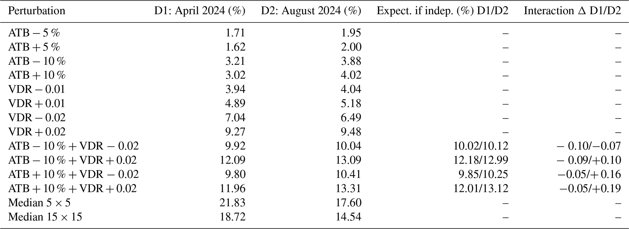
Because ATB and VDR uncertainties may occur simultaneously, four additional experiments combining the largest perturbations were performed: ATB − 10 % $/$ VDR − 0.02, ATB − 10 % $/$ VDR + 0.02, ATB + 10 % $/$ VDR − 0.02, and ATB + 10 % $/$ VDR + 0.02. Finally, the sensitivity to the preprocessing scale was investigated by replacing the reference 10 × 10 median-filter kernel with 5 × 5 and 15 × 15 kernels. All other processing and classification parameters were kept unchanged.

For each experiment, the perturbed classification was compared pixel by pixel with the reference CONIOPOL classification. Transition matrices were constructed in which each row represents a reference class and each column the class obtained after perturbation. The matrices were normalized by the total number of observations belonging to each reference class, allowing both the persistence of each classification and its redistribution toward other categories to be quantified. The complete transition matrices for April and August 2024 are provided in Appendix A (Figs. A1 and A2, respectively). For the sensitivity analysis only, an additional diagnostic category, termed “Classification loss”, was introduced. This category identifies observations that were assigned to a CONIOPOL class in the reference configuration but were no longer retained as classified pixels after perturbation. Such losses primarily arise from the spatial consistency filtering applied to the CONIOPOL classification output: perturbations of the optical parameters can modify the local distribution of classified pixels, causing some pixels to no longer satisfy the minimum relative-frequency criterion within the filtering window. The “Classification loss” is therefore not part of the operational CONIOPOL classification scheme and is used solely to quantify the fraction of reference classifications lost as a consequence of the imposed perturbations.

The overall fraction of modified classifications for each sensitivity experiment is summarized in Table 1, while the corresponding class-to-class transition matrices for April and August 2024 are shown in Figs. A1 and A2 in Appendix A, respectively. Overall, CONIOPOL showed relatively low sensitivity to ATB perturbations. For most atmospheric categories, the large majority of classifications remained unchanged under ± 5 % perturbations, and high persistence was generally maintained when the perturbation was increased to ± 10 %. The largest ATB-related changes occurred for categories close to backscatter-dependent decision boundaries, particularly smoke/marine aerosol and some mixed aerosol and hydrometeor classifications. The similarity of the results obtained for April and August indicates that this behaviour is not restricted to a particular seasonal aerosol regime.

A greater sensitivity was observed for VDR. Perturbations of ± 0.01 and ± 0.02 primarily redistributed observations between neighbouring categories separated by fixed depolarization thresholds. Negative VDR perturbations preferentially shifted classifications toward lower-depolarization categories, whereas positive perturbations promoted transitions toward categories characterized by higher depolarization. This behaviour was particularly apparent among the dust, ice/dust and ash/dust/ice categories and among neighbouring hydrometeor classes. The intermediate aerosol categories therefore play an important role in accommodating measurement variability and the natural overlap of optical properties near the classification thresholds, rather than forcing ambiguous observations directly into a single pure aerosol class.

The combined ATB–VDR experiments resulted in greater redistribution than ATB perturbations alone, but the transition patterns remained predominantly controlled by the imposed VDR perturbation (Figs. A1 and A2). At the global level, the combined response was remarkably close to that expected assuming independent ATB and VDR effects. The difference between the observed fraction of modified classifications and that predicted under independence remained below 0.2 percentage points for all combined experiments and both periods (Table 1). This suggests that interactions between ATB and VDR perturbations have only a minor influence on the overall fraction of modified classifications, although class-specific interactions remain visible in the transition matrices. Within the range of perturbations investigated here, CONIOPOL is therefore more sensitive to uncertainty in depolarization than to realistic ATB calibration biases.

VDR perturbations also affected neighbouring hydrometeor classes. In particular, positive VDR perturbations shifted part of the low-depolarization population toward higher-depolarization precipitation categories (Figs. A1 and A2). This sensitivity provides an additional potential contribution to the higher precipitation occurrence derived from CONIOPOL compared with the AWS (Sect. 4.3), as small VDR variations may cause observations close to classification thresholds to be assigned to a different hydrometeor category. However, the sensitivity experiment does not quantify how much of the observed CONIOPOL–AWS difference can be attributed to VDR uncertainty.

Changing the median-filter kernel size produced a broader redistribution across several categories than the ATB perturbations. This behaviour reflects the sensitivity of spatially and temporally heterogeneous features to the scale over which signal continuity is imposed. Smaller kernels preserve more fine-scale variability, whereas larger kernels favour spatially and temporally coherent structures at the expense of isolated or short-lived features. Nevertheless, the main classification patterns remained identifiable for both April and August.

Overall, the sensitivity analysis indicates that CONIOPOL is comparatively robust to ATB calibration uncertainties of up to ± 10 %, whereas VDR variability represents the dominant source of sensitivity among the optical parameters investigated. The effects are concentrated primarily near fixed classification boundaries and result preferentially in transitions between optically neighbouring or intermediate categories rather than arbitrary changes across the classification scheme. The filtering scale represents an additional source of variability, particularly for heterogeneous and short-lived atmospheric features. These results emphasize the importance of regular monitoring of both backscatter calibration and depolarization performance and should be considered when interpreting occurrence statistics derived from the CONIOPOL classification.

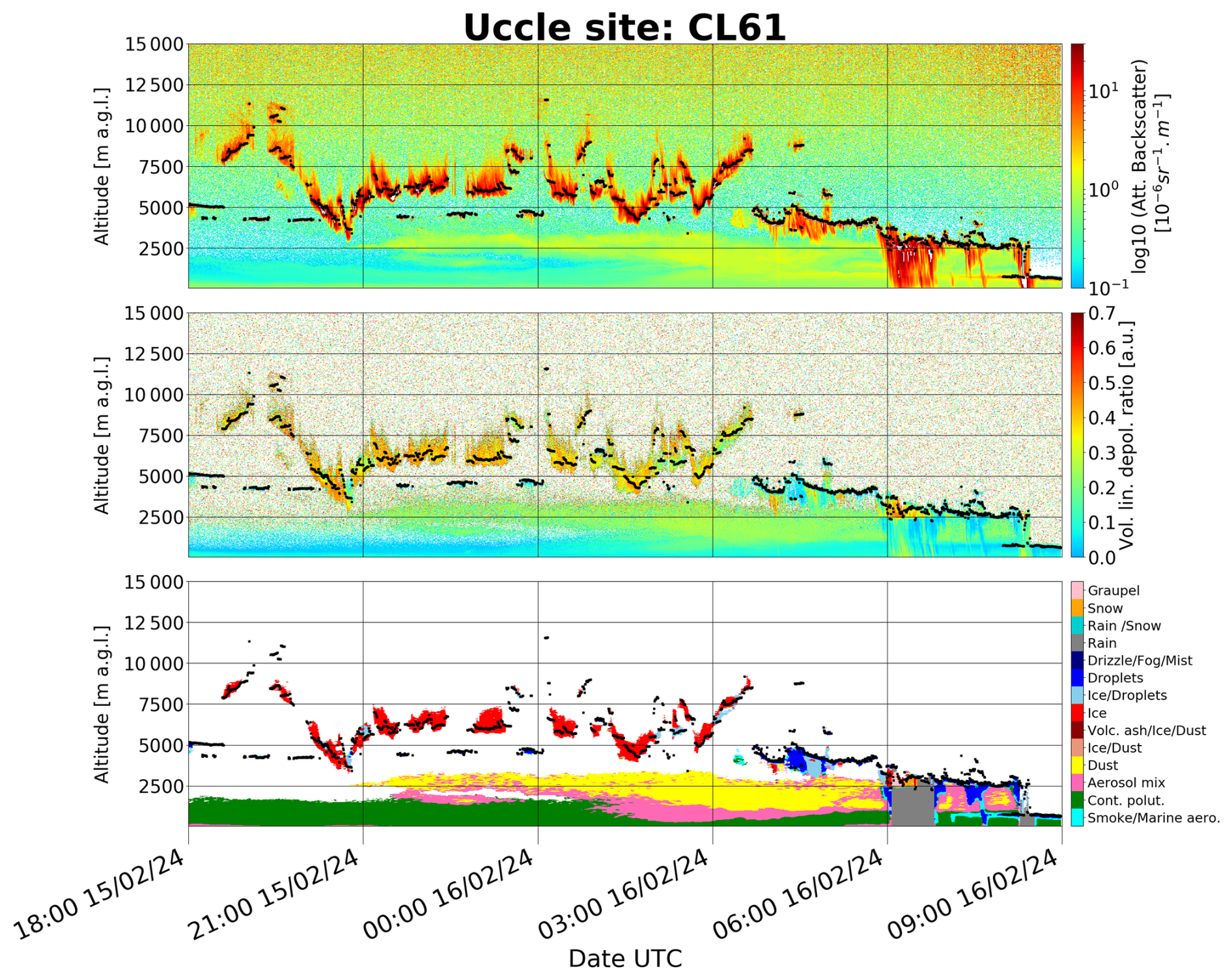
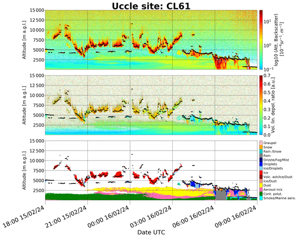
Figure 8 Raw ATB (top) and VDR (middle) observed during the night of 15–16 February 2024 in Uccle with the CL61, shown as a function of altitude and time, together with the corresponding CONIOPOL classification (bottom). The classification panel displays the identified aerosol types, hydrometeors, and cloud phases. Black dots indicate the detected CBH.

4.8 Showcase

To illustrate the practical application of the CONIOPOL classification framework, Fig. 8 presents a representative example of its output applied to CL61 measurements acquired on 16–17 February 2024. The example showcases how the algorithm interprets the raw ATB and VDR signal to produce a temporally and vertically coherent categorization of atmospheric aerosols and hydrometeors.

During the previous night and the early morning hours of 16 February, CONIOPOL detected an elevated dust plume situated near the top of the ABL. The plume exhibited weak coupling with the underlying ABL, allowing a portion of the dust to mix with background aerosols of the ABL. This interaction was accordingly classified as aerosol mix. Importantly, the plume remained aloft, suggesting limited direct influence on surface air quality during this period. The plot also shows multiple cloud layers, with CONIOPOL clearly discriminating an upper layer composed of ice crystals and a lower layer composed of supercooled liquid water, reflecting the vertical complexity of the cloud field. Precipitation features were also captured: shortly before 07:00 UTC, the algorithm identified a snow–rain transition near 2200 m. Overall, this example highlights the capability of CONIOPOL to extract fine-scale atmospheric structure from single-wavelength ALC measurements and to provide a detailed and physically consistent depiction of aerosol, cloud, and precipitation processes.

5 CAMS Global Forecast

The CAMS Global Forecast provides daily near-real-time predictions of atmospheric composition, including aerosols and reactive gases, on a global grid (Flemming et al., 2015; Peuch et al., 2022). Forecasts are produced using the ECMWF Integrated Forecasting System, which couples meteorology with aerosol and chemistry modules. Two forecast cycles are issued per day at 00:00 and 12:00 UTC, each with a native temporal resolution of 3 h and extending up to 5 d. In this study, only the first 12 h of each forecast cycle were used.

The CAMS Global Forecast was used as an independent atmospheric composition dataset to compare the aerosol environments associated with the CONIOPOL classifications. The comparison was intended to assess the physical consistency between the aerosol classes identified by CONIOPOL and the aerosol fields represented by CAMS, rather than to provide a formal validation of the algorithm. Although atmospheric composition models are affected by uncertainties in emissions, transport, and aerosol parameterizations, they provide spatially and temporally continuous aerosol fields that constitute a valuable reference for assessing the consistency of site-specific observations (Eskes et al., 2024; Flentje et al., 2021). Key aerosol species from CAMS used in this study include total dust (0.03–20 µm) mixing ratio, total sea salt (0.003–20 µm) mixing ratio, total soot (hydrophilic + hydrophobic black carbon) mixing ratio, total organic carbon (hydrophilic + hydrophobic organic matter) mixing ratio, and sulfate aerosols mixing ratio (Benedetti et al., 2009; Morcrette et al., 2009; Rémy et al., 2019).

Compared to the CAMS reanalysis, which provides a temporally consistent retrospective dataset primarily intended for climate studies and long-term analysis, the CAMS forecast product is better suited for short-term monitoring of wildfire smoke, dust events, and air quality. Moreover, the reanalysis was not available at the time this study was initiated, making the forecast product the best option for timely analysis.

6 Results

6.1 CONIOPOL output analysis

The analysis of CONIOPOL output was carried out over a complete annual cycle. Although most aerosols were confined to the ABL and the adjacent lower free troposphere, the entire profile was analysed to include all detection classes, including high-altitude ice crystals. The occurrence statistics are subject to the inherent limitations of the CL61: limited sensitivity to weak aerosol loadings and signal extinction above optically thick clouds. Consequently, the reported occurrences represent detections within the observable atmospheric column rather than the true atmospheric occurrence of each category.

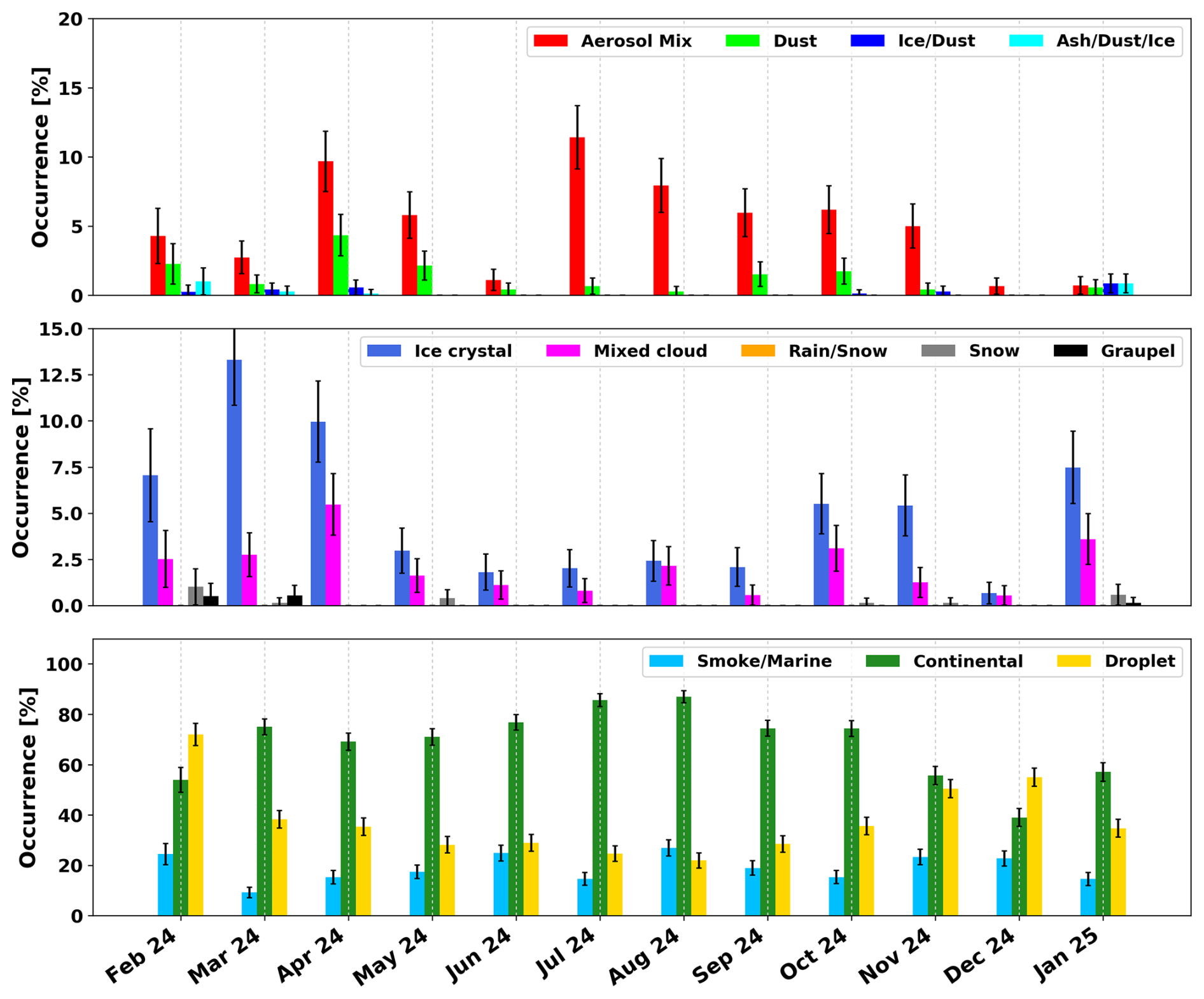
Figure 9 Monthly occurrence (%) of the different CONIOPOL-detected classes between February 2024 and January 2025. The occurrence analysis was performed using the full CL61 vertical profile (50 m–15.4 $\mathrm{km}\mathrm{a}.\mathrm{g}.\mathrm{l}.$). Top panel: occurrence of mixed aerosols, dust, ice/dust, and ash/dust/ice. Middle panel: occurrence of ice crystals, mixed-phase clouds, rain/snow, snow and graupel. Bottom panel: occurrence of smoke/marine aerosols, continental aerosols, and liquid cloud droplets. Monthly occurrences were computed as the fraction of hourly periods for which a given atmospheric target was detected in at least 60 % of the available observations within that hour. Error bars represent the 95 % confidence intervals.

6.1.1 Occurrence analysis

Figure 9 presents the monthly distribution of aerosol, cloud phase and solid precipitation occurrences throughout the study period. For each category, the monthly occurrence was calculated as the percentage of hourly profiles in which the corresponding category was detected in at least 60 % of the observations within that hour, relative to the total number of hourly profiles acquired during the month. Because multiple targets can coexist vertically within a single profile, summed occurrences across categories may exceed 100 %.

Throughout the year, continental aerosol classification was most frequently observed, with monthly occurrences consistently exceeding 50 % and reaching peaks of approximately 85 % in July and August. The second most prevalent category was represented by smoke/marine aerosols, with monthly occurrences generally ranging from approximately 10 %–27 %. Although some month-to-month variability was observed, no clear seasonal cycle emerged from the dataset. Mixed aerosols represented the third most frequently detected aerosol category and exhibited a more pronounced seasonal variability, with distinct peaks in April, July, and August, where occurrences reached approximately 10 %–12 %. Dust was observed at moderate frequencies, primarily during spring (April–May) and autumn (September–October). Ice/dust and ash/dust/ice mixtures were only occasionally identified, generally accounting for less than 1 % of the observations.

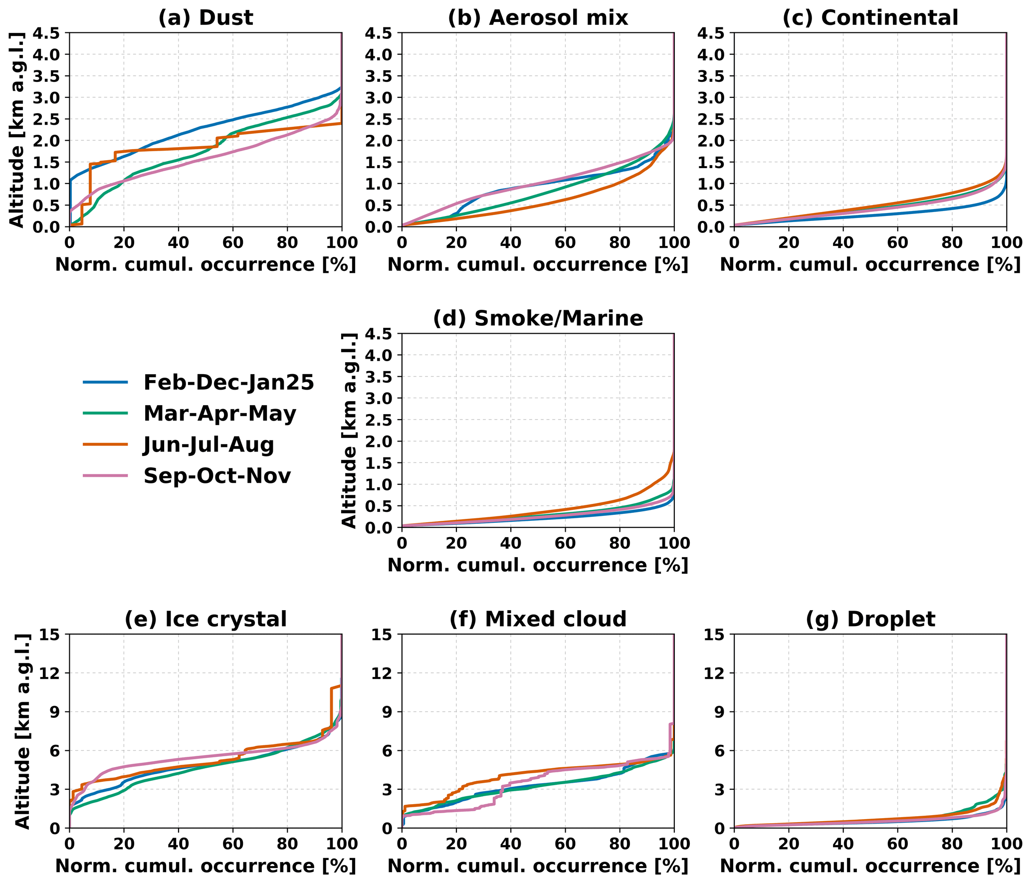
Figure 10 Seasonal normalized cumulative occurrence profiles of the main atmospheric target classes identified by CONIOPOL: (a) dust, (b) aerosol mix, (c) continental aerosol, (d) smoke/marine, (e) ice crystals, (f) mixed-phase clouds, and (g) liquid clouds. The profiles represent the normalized cumulative occurrence of detections from the surface (50 m) to a given altitude for the four climatological seasons: (February–December–January 2025 (blue), March–April–May (green), June–July–August (orange), and September–October–November (purple). For each altitude, the cumulative occurrence corresponds to the fraction of all detections located below that altitude and is normalized to 100 % at the highest detected altitude. Aerosol categories are displayed up to 4.5 km, whereas cloud and ice crystal categories are shown up to 15 km.

Regarding hydrometeors, ice crystals exhibited a marked seasonal cycle, with maxima during late winter–early spring and a secondary maximum during autumn–early winter, while summer occurrences remained comparatively low. Mixed-phase clouds were detected less frequently, with monthly occurrences generally ranging between approximately 1 % and 5 %. Their highest frequencies were recorded during April and again from October to January, following a seasonal evolution similar to that of ice crystals but with substantially lower occurrences. Liquid cloud droplets represented by far the most abundant hydrometeor category. Monthly occurrences varied between approximately 20 % and 70 %, with the highest frequencies observed during February 2024 and November–December 2024. These periods coincide with enhanced low-level cloudiness and more frequent precipitation events (Fig. 4). In contrast, solid precipitation remained relatively uncommon throughout the study period. Snow and graupel occurrences generally remained below 1 %, although isolated increases were observed during February–March 2024 and January 2025, reflecting the few winter precipitation events captured by CONIOPOL.

6.1.2 Vertical cumulative analysis

The examination of the vertical distribution of each target type in relation to its seasonal variability provides valuable insight into both the dominant altitude ranges and their temporal evolution of occurrence throughout the year. To this end, Fig. 10 presents the seasonal normalized cumulative occurrence for the main aerosol and hydrometeor categories. Only persistent detections, defined as an atmospheric target occupying at least 60 % of the profiles within an hour, were considered. Normalization allows direct comparisons between seasons despite differences in detection frequency and provides a robust representation of the vertical structure of aerosols and hydrometeors (Baars et al., 2012; Illingworth et al., 2007).

The dust category exhibited the largest seasonal variability among the aerosol classes. During winter (December–January–February), dust layers frequently extended above 3 km, whereas during summer (June–July–August) most detections remained confined below approximately 2.5 km. Spring (March–April–May) and autumn (September–October–November) displayed intermediate behaviour.

A marked seasonal dependence was also observed for the vertical distribution of mixed aerosols. During winter and autumn, the normalized cumulative occurrence profiles evolved with altitude in a manner similar to those of dust, indicating a comparable vertical distribution. In contrast, during spring and summer, the mixed aerosol profiles more closely resembled those of continental aerosols, although a greater vertical extent was observed, with detections reaching approximately 2.5 km compared with about 1.5 km for continental aerosols.

Continental aerosols remained predominantly confined to the lower troposphere throughout the year, with a stronger confinement during winter and more than 90 % of detections occurring below approximately 1.5 km in the other seasons. Smoke/marine exhibited a similar seasonal evolution but remained even more confined to the lowest atmospheric layers, with most detections below 1 km except during summer, when smoke layers occasionally extended above 1.5 km.

The vertical distributions of ice crystals and mixed-phase clouds extended well above those of aerosols, reaching altitudes of approximately 10–12 km. Although the overall shape of the normalized cumulative occurrence profiles remained relatively similar throughout the year, a slightly larger fraction of high-altitude ice crystal detections was observed during summer. Mixed-phase clouds were mostly confined below approximately 6 km. In contrast, liquid clouds were largely restricted to the lower troposphere, with most detections occurring below approximately 3–4 km and only limited seasonal variability being observed.

6.1.3 Conditional comparison with CAMS forecast

Because CAMS provides grid-cell averaged aerosol mixing ratios whereas CONIOPOL identifies atmospheric targets from high-resolution ALC observations, the comparison was performed conditionally rather than on a point-by-point basis. CAMS aerosol mixing ratios extracted from the model grid point closest to Uccle were analysed according to the corresponding CONIOPOL aerosol classifications to assess whether the different CONIOPOL classes are consistently associated with physically distinct aerosol environments represented by CAMS. Since CAMS aerosol profiles are available every 3 h, the corresponding CONIOPOL observations were aggregated over the same period. This interval was divided into three consecutive 1 h periods. For each altitude level, an hourly period was considered positive for a given aerosol category when the category was detected during at least 60 % of the available CONIOPOL observations. A CAMS profile was associated with a CONIOPOL aerosol category only when this criterion was fulfilled in at least two of the three hourly periods, thereby retaining only persistent aerosol layers and reducing the influence of short-lived detections. Owing to its much higher temporal and vertical resolution, CONIOPOL additionally provides information on the occurrence and fine-scale vertical structure of aerosol layers that cannot be resolved by the 3-hourly, grid-cell averaged CAMS forecasts.

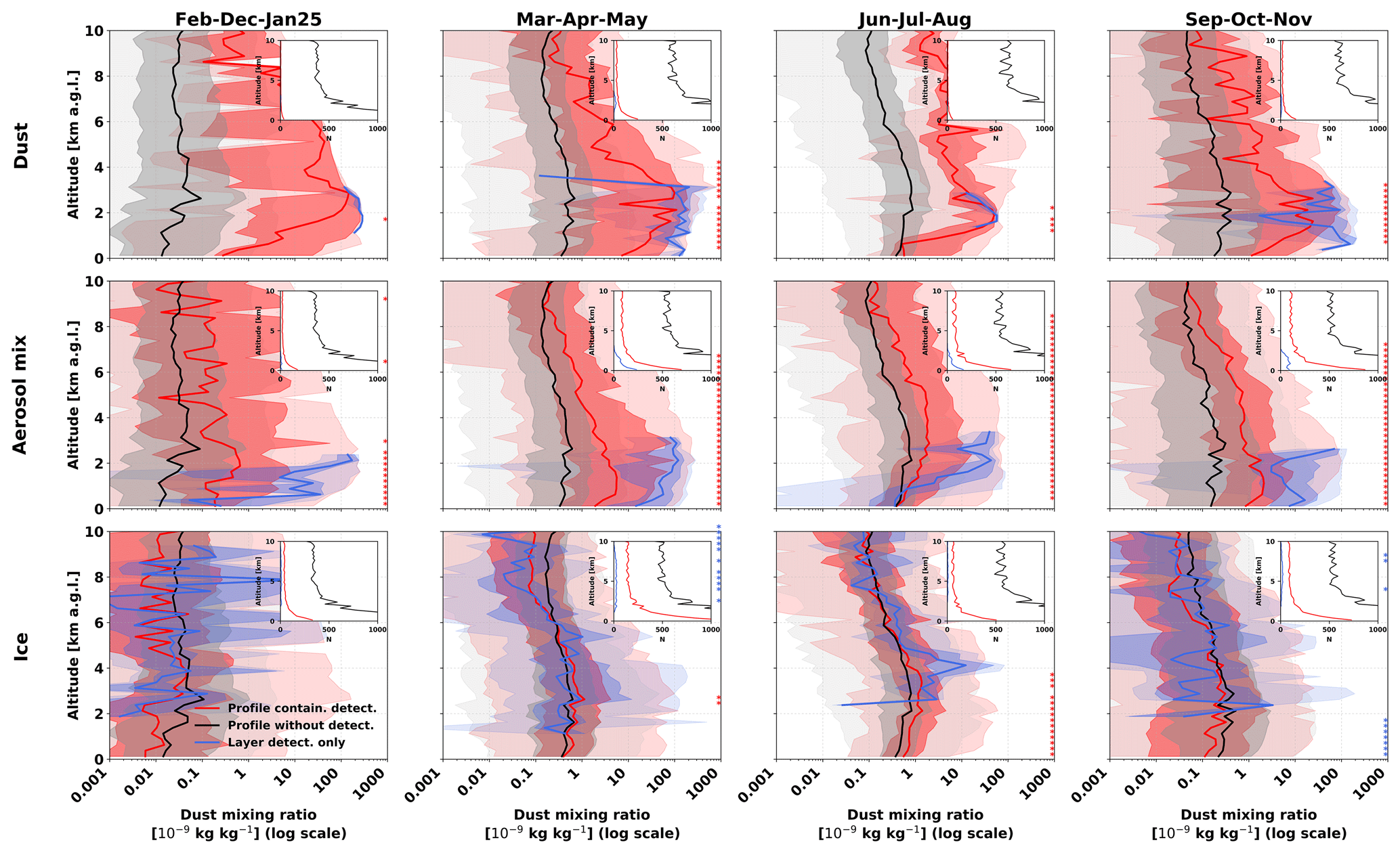
Figure 11 Seasonal comparison between CONIOPOL classifications and CAMS total dust mixing ratios. Vertical profiles of CAMS total dust mixing ratio are shown for three groups: profile containing detection, corresponding to CAMS profiles for which the considered CONIOPOL category was detected at least once within the atmospheric column (red); layer detection only, corresponding to individual altitude levels where the considered category was detected by CONIOPOL irrespective of the classification of the remainder of the profile (blue); and profile without detection, corresponding to profiles without any detection of the considered category (black). Solid lines represent the median, dark shading the interquartile range (25th–75th percentiles), and light shading the 5th–95th percentile range. Asterisks indicate altitude intervals where the CAMS mixing-ratio distributions associated with profile containing detection and profile without detection differ significantly according to a two-sided Mann–Whitney U test (p < 0.001). Red asterisks indicate that the median mixing ratio is higher for the profile containing detection group than for the profile without detection group, whereas blue asterisks indicate the opposite. The sample size (N) for each group is reported in the upper-left corner of each subplot, while the number of samples available within each 250 m altitude interval is shown for the profile containing detection (red), layer detection only (blue), and profile without detection (black) groups. The four vertical panels correspond to the December–February (February–December–January 2025), March–May (March–April–May), June–August (June–July–August), and September–November (September–October–November) periods. Results are shown for the dust, aerosol-mix, and ice-crystal categories.

For each season, CAMS vertical profiles were grouped according to the corresponding CONIOPOL classifications into three categories: (i) full profiles for which the considered aerosol category was detected at least once within the atmospheric column, (ii) full profiles without any detection of the considered category, and (iii) individual altitude levels where the considered category was detected, irrespective of the classification of the remainder of the profile. For the statistical analysis, CAMS data were aggregated into successive 250 m altitude intervals in order to account for the differing vertical resolutions of CAMS and CONIOPOL and to ensure a sufficient number of samples within each layer. Because the CAMS model uses terrain-following hybrid vertical levels whose spacing increases with altitude, the number of available samples within each 250 m interval gradually decreases with height. Figure 11 presents the seasonal vertical distributions of CAMS dust mixing ratios conditioned on the CONIOPOL dust, aerosol-mix and ice-crystal classifications.

For the dust category, both full-profile and layer-only detections were consistently associated with substantially higher CAMS dust mixing ratios than non-detection cases, with the clearest differences occurring below approximately 3 km, where most altitude intervals showed statistically significant differences. In most seasons, layer-only detections exhibited higher median dust mixing ratios than full-profile detections, although substantial overlap between the distributions remained. Overall, these results demonstrate that CONIOPOL dust detections preferentially occur under atmospheric conditions characterized by enhanced mineral dust loading.

The aerosol-mix category exhibited an intermediate behaviour, with CAMS dust mixing ratios generally higher than for non-detection profiles but lower than those associated with the dust category. Statistically significant differences between detection and non-detection populations were also observed over a broader altitude range in several seasons. This suggests that the aerosol-mix classification retains sensitivity to the presence of mineral dust even under conditions where the dust contribution is weaker or mixed with other aerosol components. The more limited statistical significance of the dust category at higher altitudes should not necessarily be interpreted as a weaker association with mineral dust, as it may partly reflect the smaller number of dust detections and the resulting greater sampling variability. Together, these results support the interpretation of the aerosol-mix category as representing aerosol populations containing a detectable mineral dust contribution mixed with less-depolarizing aerosol types.

For the ice-crystal category, CAMS dust mixing ratios generally showed substantial overlap between detection and non-detection populations, indicating no systematic association between CONIOPOL ice-crystal detections and enhanced mineral dust loading. Nevertheless, occasional enhancements in CAMS dust mixing ratios, particularly during summer, suggest that mineral dust and ice clouds may coexist within the same atmospheric column. In the other seasons, ice-crystal detections were generally associated with lower dust mixing ratios than non-detection cases over several altitude ranges, with some differences being statistically significant. Overall, these results suggest that most ice-crystal detections occurred under relatively weak mineral dust conditions, while occasional dust-rich situations cannot be excluded.

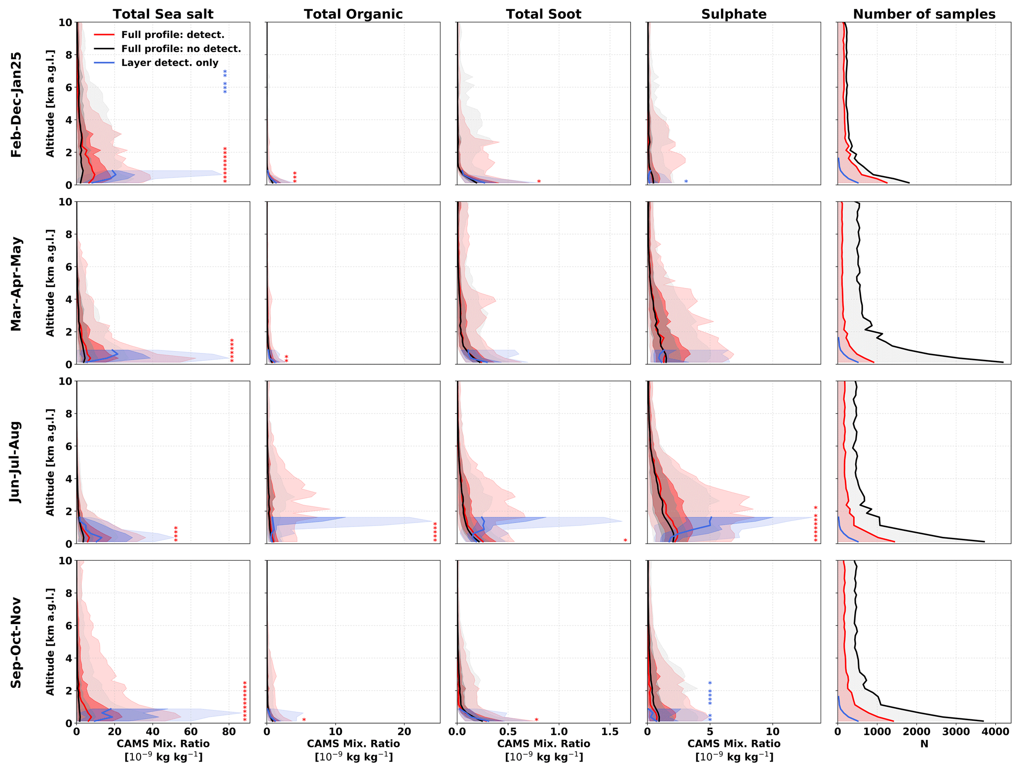
Figure 12 Seasonal comparison between CONIOPOL smoke/marine aerosol classifications and CAMS aerosol mixing ratios for total sea salt, total organic carbon, total soot, and sulphate. Vertical profiles of CAMS aerosol mixing ratios are shown for three groups: profile containing detection, corresponding to CAMS profiles for which the smoke/marine category was detected at least once within the atmospheric column (red); layer detection only, corresponding to individual altitude levels where the smoke/marine category was detected by CONIOPOL irrespective of the classification of the remainder of the profile (blue); and profile without detection, corresponding to profiles without any smoke/marine detection (black). Solid lines represent the median, dark shading the interquartile range (25th–75th percentiles), and light shading the 5th–95th percentile range. Asterisks indicate altitude intervals where the CAMS mixing-ratio distributions associated with profile containing detection and profile without detection differ significantly according to a two-sided Mann–Whitney U test (p < 0.001). Red asterisks indicate higher median mixing ratios for the profile containing detection group than for the profile without detection group, whereas blue asterisks indicate the opposite. The right-hand column shows the number of samples (N) available within each 250 m altitude interval for the profile containing detection (red), layer detection only (blue), and profile without detection (black) groups. The four rows correspond to the December–February (February–December–January 2025), March–May (March–April–May), June–August (June–July–August), and September–November (September–October–November) periods.

Figure 12 presents the seasonal comparison between the CONIOPOL smoke/marine category and the corresponding CAMS aerosol species (sea salt, organic matter, soot, and sulfate). For total sea salt, higher CAMS mixing ratios were consistently associated with CONIOPOL detections than with non-detection cases within approximately the lowest kilometer of the atmosphere, where statistically significant differences were frequently observed. Above this altitude, the distributions became increasingly similar, consistent with the predominantly ABL occurrence of sea-salt aerosols.

In contrast, total organic carbon, total soot, and sulphate were consistently associated with enhanced CAMS mixing ratios over a much deeper vertical extent, particularly during June–August. Similar to the dust category, the largest contrasts with the non-detection profile were observed within the lower troposphere, while statistically significant differences frequently extended above 1 km, consistent with the long-range transport of biomass-burning aerosols. Unlike the dust category, layer-only detections exhibited sulphate mixing ratios comparable to those associated with profile-containing detections, particularly during summer.

7 Discussion

Overall, the results highlight clear seasonal and vertical patterns in the occurrence and distribution of aerosols and hydrometeors over the study site. The conditional comparison with the CAMS Global Forecast reveals a generally consistent correspondence between the aerosol environments identified by CONIOPOL and those represented by the model, despite the fundamentally different nature of the two datasets. The analyses collectively indicate that depolarizing aerosols such as dust and mixed aerosols exhibit distinct altitude-dependent signatures and temporal variability, while continental and low-depolarizing aerosols remain largely confined to the ABL. The statistically significant differences observed between the CAMS aerosol mixing-ratio distributions associated with the various CONIOPOL classes support the interpretation that the classifications correspond to physically distinct aerosol environments. However, this comparison should not be regarded as a formal validation, as CAMS provides modelled aerosol mixing ratios at coarse spatial and temporal resolution, whereas CONIOPOL delivers observation-based target classifications at high temporal and vertical resolution. Consequently, both datasets provide complementary rather than directly comparable information. It should also be noted that the present analysis is based on a single year of observations at a single site, which limits its representativeness but provides an unprecedented temporally continuous record for the region. In addition, the sensitivity analysis showed that CONIOPOL remained comparatively robust to the ATB calibration uncertainties of up to ± 10 %, whereas VDR variability represented the dominant source of sensitivity among the optical parameters investigated. Classification changes occurred primarily for observations close to fixed decision thresholds and generally resulted in transitions between neighbouring categories rather than arbitrary changes across the classification scheme. The filtering scale introduced an additional source of variability, particularly for heterogeneous and short-lived atmospheric features. These sensitivities should therefore be considered when interpreting individual detections and occurrence statistics. With the aim of further assessing the physical consistency of CONIOPOL, the following discussion places these findings in the context of previous studies, exploring the physical and meteorological processes underlying the observed seasonal patterns and altitude dependencies.

7.1 Aerosol

7.1.1 Depolarizing targets

Comparing our results with previous studies conducted in Western and Central Europe remains challenging. First, the aerosol classification scheme employed in our analysis does not perfectly align with those used in other studies, making direct comparisons difficult. Second, unlike many earlier works that rely on campaign-based or discontinuous datasets, our study provides continuous, uninterrupted temporal coverage, which helps reduce potential sampling biases. Moreover, to our knowledge, no study covering the entire year 2024 has yet been published for Western and Central Europe, limiting the availability of recent reference data. Nevertheless, despite natural variability, previous studies can serve as useful benchmarks for assessing whether the characteristics of the aerosol categories detected by CONIOPOL are consistent with earlier observations.

For the dust category, the altitudes of the plumes detected by CONIOPOL fall within the range observed at Palaiseau, with heights between 400 and 4000 m (Papayannis et al., 2008). Regarding the seasonality of dust plumes, our study shows the highest occurrences in February, March, May, September, and October, rather than during the summer months. This contrasts with Marinou et al. (2017), who reported stronger dust activity over Central and Western Europe during spring and summer, based on a 9-year dataset that provides a more robust climatological reference than our 1-year analysis. In our case, the highest frequency of the aerosol mix category occurred in June, which may correspond to one or more dust intrusion events combined with other aerosol types. This interpretation is consistent with the CAMS comparison analysis, which indicates that the aerosol mix category was associated with noticeably higher CAMS dust mixing ratio values compared to periods without depolarizing target detections. However, these values remained well below those observed when CONIOPOL explicitly detected dust, suggesting that the aerosol mix class likely represents episodes of partial or diluted dust intrusions combined with other aerosol types. Such mixing becomes increasingly pronounced with the atmospheric transport distance from the source region (Dall'Osto et al., 2010). Furthermore, it is also possible that dust transport toward Western Europe was reduced in 2024, due to more efficient removal processes and large-scale circulation patterns (e.g., Schepanski et al., 2009) that favored eastward transport. Indeed, Ionita and Nagavciuc (2025) reported that the summer of 2024 was marked by unprecedented heatwaves and exceptionally dry conditions in Eastern Europe, linked to a persistent high-pressure system over the eastern continent and a low-pressure anomaly over the central North Atlantic (Ionita et al., 2025). These synoptic features likely enhanced the eastward advection of Saharan dust while limiting its transport toward Western Europe. It should also be noted that aerosol layers located above optically thick clouds or embedded within cloud layers cannot be observed by the ALC. Consequently, some dust events, as well as other aerosol episodes, are likely to be underrepresented in the CONIOPOL climatology.

The comparison reveals a clear altitude dependence in the relationship between CAMS dust mixing ratios and positive CONIOPOL dust detections. For comparable CAMS dust mixing ratios, dust layers were more frequently detected by CONIOPOL within the lower atmosphere than above approximately 2 km. Two complementary mechanisms likely contribute to this behaviour. First, global aerosol models such as CAMS often struggle to reproduce these near-surface concentrations accurately because of coarse vertical resolution, simplified ABL parameterizations, and uncertainties in deposition and transport processes (Huneeus et al., 2011; Zender et al., 2003). Near the surface, mineral dust is strongly influenced by gravitational settling, dry and wet deposition, turbulence, and frictional effects (Seinfeld and Pandis, 1998), while virga-induced turbulence may further redistribute dust vertically during sublimating precipitation events (Karle et al., 2023). Second, the detection capability of the CL61 progressively decreases with altitude because the ALC signal-to-noise ratio degrades with increasing range and atmospheric attenuation, reducing the sensitivity to optically thin aerosol layers aloft. This general limitation applies to all aerosol categories but is particularly relevant for elevated mineral dust layers. Consequently, dust layers associated with similar CAMS mixing ratios may be more readily detected close to the surface than at higher altitudes. The observed discrepancies should therefore not be interpreted as deficiencies of either dataset but rather as a consequence of their different representativeness and measurement principles. CAMS provides grid-cell averaged aerosol mixing ratios representative of the large-scale atmospheric environment, whereas CONIOPOL identifies individual aerosol layers from high-resolution observations. Despite potential mismatches during the onset and dissipation of dust events owing to the different temporal resolutions of the datasets, the overall correspondence remains robust. Periods without depolarizing aerosol detections in CONIOPOL generally coincide with low or negligible CAMS dust mixing ratios, whereas positive CONIOPOL dust detections are consistently associated with enhanced dust concentrations aloft. These statistically significant differences support the capability of CONIOPOL to identify physically meaningful mineral dust layers despite the intrinsic differences between the observational and modelling approaches.

The enhanced occurrence of the mixed aerosol category during spring may also partly reflect the presence of pollen. As discussed in Sect. 4.4, pollen exhibits depolarization ratios that overlap with those assigned to the mixed aerosol category and therefore cannot always be distinguished from other weakly depolarizing aerosol types using a single-wavelength polarization-enabled ALC. This interpretation is further supported by the occasional occurrence of a pronounced diurnal detection pattern (results not shown) consistent with the diurnal cycle of pollen emissions reported in previous lidar studies (Bohlmann et al., 2019, 2021; Noh et al., 2013; Sicard et al., 2016). Additional evidence is provided by the normalized cumulative occurrence profiles (Fig. 9). During winter and autumn, the vertical distribution of the mixed aerosol category closely resembles that of the dust category, suggesting that these observations are frequently associated with diluted or partially mixed mineral dust layers. In contrast, during spring and summer, the cumulative occurrence profiles become more similar to those of continental aerosols, although the mixed aerosol category consistently exhibits an intermediate vertical distribution between the continental and dust categories. This behaviour may reflect the greater depth of the ABL during spring and summer dust episodes. More importantly, the transition from dust-like vertical profiles in winter and autumn to profiles approaching those of continental aerosols during spring and summer suggests that the dominant aerosol population within this class also changes seasonally, with an increasing contribution from boundary-layer aerosols, among which pollen is a plausible contributor. This interpretation is further supported by the enhanced occurrence of the mixed aerosol category during the main pollen season in Belgium (Hoebeke et al., 2018; Verstraeten et al., 2025; de Weger et al., 2021). However, the June minimum does not coincide with the transition between tree and grass pollen emissions, which typically occurs in May (Hoebeke et al., 2018), suggesting that meteorological conditions and the contribution of other aerosol types also influence the seasonal behaviour within this category. Furthermore, because pollen optical properties vary considerably with species, particle size, morphology, and atmospheric conditions, not all pollen events are expected to be classified within the mixed aerosol category. This uncertainty reflects an inherent limitation of single-wavelength polarization-enabled ALC, which cannot unambiguously distinguish weakly depolarizing biogenic particles, such as pollen, from other aerosol types exhibiting similar optical properties.

7.1.2 Weakly depolarizing targets

Automatic detection of weakly depolarizing targets using a single-wavelength polarization-enabled ALC remains inherently challenging. Compared with depolarizing aerosols, the comparison with CAMS was more difficult to interpret when assessing the classification performance of CONIOPOL. This limitation is likely attributable, in part, to the complex processes occurring within the lowest layers of the atmosphere, which are frequently underrepresented in global models, including CAMS, as previously noted. This issue is particularly pertinent given that the majority of CONIOPOL detections of the smoke/marine aerosol category were confined to the lowest atmospheric layers, where model uncertainties and the influence of near-surface processes are most pronounced.

The normalized cumulative occurrence profiles provide additional insight into the vertical distribution of the weakly depolarizing aerosol categories. Although the continental and smoke/marine aerosol categories exhibit a broadly similar seasonal evolution, reflecting the seasonal development of the ABL, the smoke/marine category remains consistently confined to lower altitudes. Most smoke/marine detections occur within the lowest atmospheric layers, whereas continental aerosols frequently extend to approximately 1.5 km. This stronger confinement is consistent with the predominant influence of the marine boundary layer, where sea-salt aerosols are generated at the ocean surface and generally remain restricted to the lowest part of the atmosphere (Boyouk et al., 2011). During summer, however, the smoke/marine category exhibits a greater vertical extent, likely reflecting both the seasonal deepening of the ABL and the contribution of elevated wildfire smoke transported within the free troposphere.

Detection of marine or sea salt aerosols is especially challenging due to their weak depolarization signal, hygroscopic growth, and frequent mixing with other aerosol types within the ABL. These factors significantly limit the sensitivity and classification accuracy of single-wavelength ALC system such as CONIOPOL (Ferrare et al., 2023; Haarig et al., 2017; Klingebiel et al., 2019). The complex morphology and humidity-dependent size variability of sea-salt particles further increase optical retrieval uncertainties and may lead to partial misclassification with other weakly depolarizing aerosols (Ferrare et al., 2023; Haarig et al., 2017) .

At higher altitudes, however, the comparison with CAMS, particularly during summer, supports the capability of CONIOPOL to identify elevated smoke plumes. Corresponding CAMS fields indicate that these plumes are frequently associated not only with enhanced soot concentrations but also by elevated concentrations of sulfate and total organic matter mixing ratios. This composition reflects the multiphase chemistry of biomass-burning aerosols, which release a mixture of black carbon, organic carbon, and sulfate precursors. These precursors undergo atmospheric oxidation to form secondary aerosols, thereby enhancing the total aerosol load at higher altitudes (Reid et al., 2005; Souri et al., 2017).

The occurrence of the continental aerosol category enhanced during summer, consistent with numerous observations across Europe (Freney et al., 2011; Mattis et al., 2008; Pio et al., 2007; Putaud et al., 2010). These studies consistently show that photochemical activity and secondary aerosol formation intensify during the warmer months, when elevated solar radiation and temperature accelerate oxidation of gaseous precursors, producing sulfates, nitrates, and secondary organic aerosols (SOA). The normalized cumulative occurrence profiles further indicate that continental aerosols remain predominantly associated with the ABL, exhibiting a shallower vertical distribution during winter and a greater vertical extent during spring and summer, consistent with the seasonal evolution of ABL depth.

7.2 Cloud phase

Beyond aerosol classification, the cloud-phase and precipitation classifications provide an additional opportunity to evaluate the physical consistency of CONIOPOL. The normalized cumulative occurrence profiles are particularly valuable in this respect, as they reveal the expected vertical organization of the different hydrometeor categories. Ice crystals category exhibit the largest vertical extent, with cumulative occurrence profiles remaining progressive up to approximately 10–12 km throughout the year, consistent with their association with cirrus and deep ice clouds. In contrast, the mixed cloud category displays a similar profile shape in the lower troposphere but approaches an asymptotic limit around 5–6 km, indicating that mixed-phase clouds are predominantly confined to the middle troposphere. Liquid clouds category exhibit a much steeper cumulative occurrence profile, with most detections occurring below approximately 3–4 km, demonstrating that liquid clouds remain largely restricted to the lower troposphere. The clear separation between the cumulative occurrence profiles of the three cloud-phase categories is fully consistent with the expected vertical stratification of cloud phase in the atmosphere and therefore provides additional confidence in the physical consistency of the CONIOPOL cloud classification.

Although ice crystals were generally detected at much higher altitudes than dust plumes, periods of ice crystal detections occasionally coincided with elevated CAMS dust mixing ratios, particularly during summer. Although this comparison does not demonstrate a direct interaction between mineral dust and ice crystals, it is consistent with previous studies identifying mineral dust as an efficient source of ice-nucleating particles (Chatziparaschos et al., 2025). Likewise, Brunner et al. (2021) showed that transported mineral dust can trigger ice crystal formation at cirrus altitudes, with the resulting ice particles subsequently sedimenting through virga into lower atmospheric layers.

8 Conclusion

The CONIOPOL algorithm, applied to single-wavelength ALC observations from the Vaisala CL61, provides a robust foundation for establishing a long-term and coherent climatology of aerosol, cloud and precipitation occurrence and variability at a measurement site. Despite their spectral limitations, polarization-enabled ALCs provide continuous, high vertical resolution observations that make them valuable tools for operational atmospheric monitoring and long-term climatological studies.

CONIOPOL provides physically consistent discrimination among major aerosol categories, including dust, mixed aerosols, smoke/marine aerosols, and continental aerosols, while also providing physically consistent cloud-phase and precipitation classifications. The sensitivity analysis further showed that CONIOPOL is comparatively robust to realistic ATB calibration biases, whereas VDR variability constitutes the dominant source of sensitivity among the optical parameters investigated, in particular for observations close to classification thresholds. The comparison with CAMS demonstrates strong agreement for transported aerosol layers, particularly mineral dust and smoke, whereas the normalized cumulative occurrence profiles reveal realistic seasonal and vertical structures for both aerosols and hydrometeors. Together, these results demonstrate that continuous polarization-enabled ALC observations provide scientifically meaningful information despite their limited spectral information.

The threshold values adopted in CONIOPOL are primarily intended for regional background observations and long-range transported aerosol layers. Their direct application in the immediate vicinity of strong local emission sources (e.g. volcanic eruptions, intense wildfire plumes or regions with exceptionally high pollen concentrations) should therefore be approached with caution, as freshly emitted particles often exhibit optical properties that differ from those of aged and well-mixed aerosols.

The relatively low acquisition and maintenance costs of polarization-enabled ALCs, combined with their straightforward 24/7 operational capability, make CONIOPOL a valuable tool for air quality monitoring. In particular, it enables real-time identification of aerosol plumes interacting with the ABL, providing information that complements numerical models and supports model evaluation and forecasting.

However, the results presented here are derived from a single site, which, while representative, cannot by itself fully validate the CONIOPOL algorithm under diverse meteorological and aerosol conditions. Expanding the analysis to multiple sites equipped with polarization-enabled ALCs – ideally covering different climatic and aerosol regimes – would provide a more comprehensive evaluation of the algorithm's performance and improve the robustness of its climatological applications.

Looking ahead, extending CONIOPOL to additional CL61 sites and combining its classifications with complementary observations from ACTRIS multi-wavelength polarization lidars, EarthCARE ATLID, and the new ACTRIS Aerosol In-Situ National Facility at Uccle will provide valuable opportunities for validating aerosol types, optical properties, and particle size distributions. Such synergies will strengthen confidence in CONIOPOL, improve model evaluation – particularly within the ABL – and advance our understanding of aerosol variability and aerosol–cloud–radiation interactions relevant for both air quality and climate applications.

Appendix A

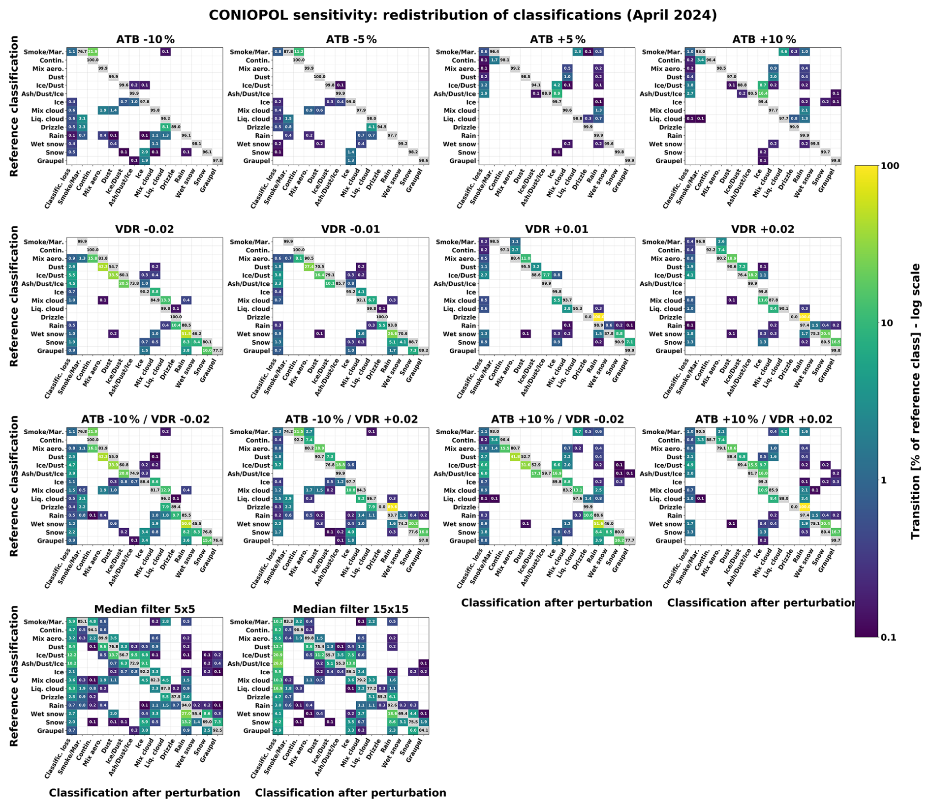
Figure A1 Sensitivity of CONIOPOL classifications to perturbations of the optical parameters and median-filter window for April 2024. Each panel shows the transition matrix between the reference CONIOPOL classification (rows) and the classification obtained after perturbation (columns). Cell values indicate the percentage of observations from each reference class assigned to the corresponding class after perturbation. Grey diagonal cells represent classifications that remain unchanged, whereas coloured off-diagonal cells indicate redistribution toward another category. “Classification loss” denotes reference classifications that are no longer retained after perturbation following the spatial consistency filtering. Transitions below 0.1 % are not displayed. Colours represent the percentage of the reference class on a logarithmic scale from 0.1 % to 100 %. The first and second rows show the sensitivity to ATB and VDR perturbations, respectively; the third row shows combined ATB–VDR perturbations; and the fourth row shows the sensitivity to the median-filter window size relative to the reference 10 × 10 kernel.

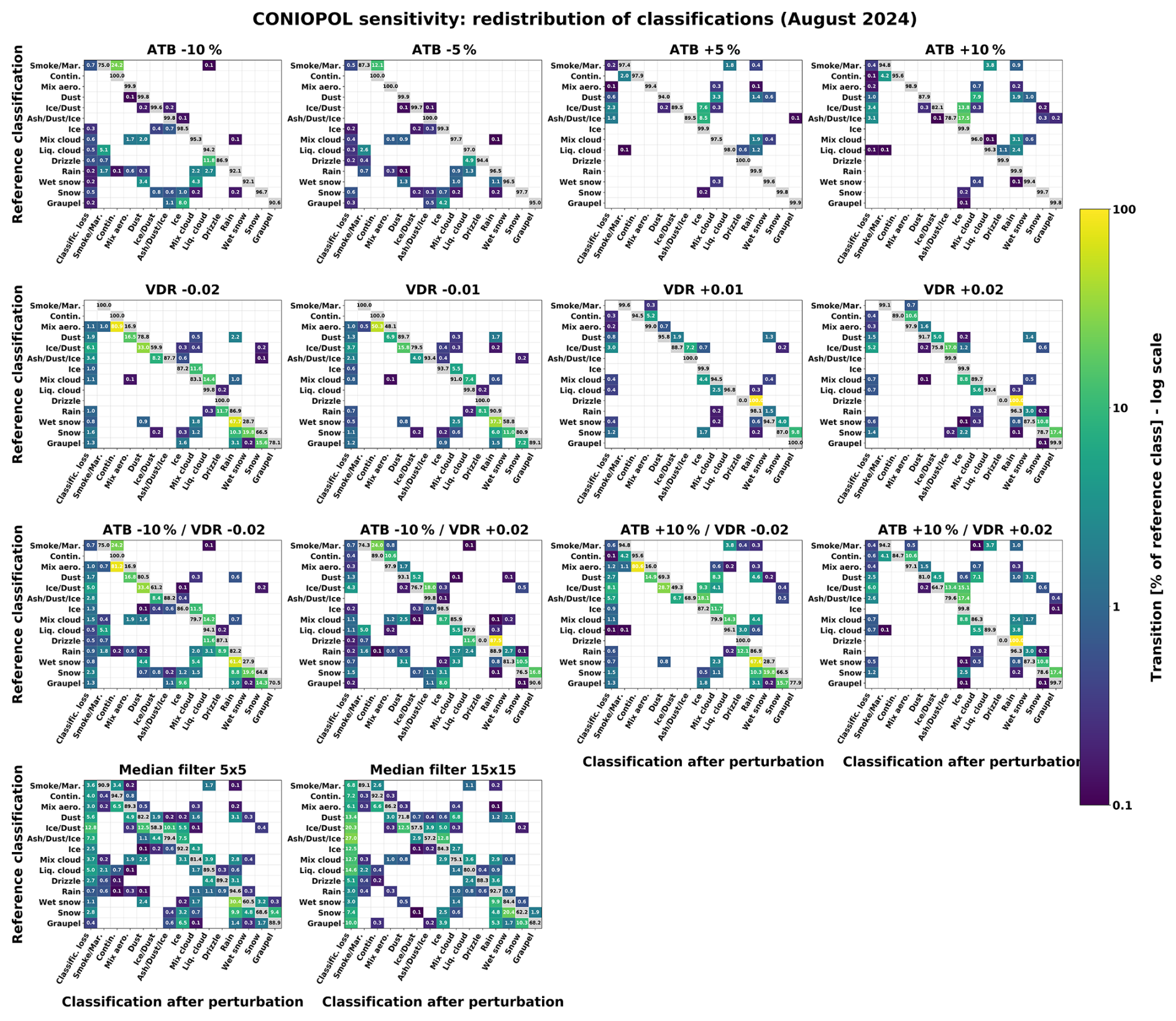
Figure A2 Sensitivity of CONIOPOL classifications to perturbations of the optical parameters and median-filter window for August 2024. Each panel shows the transition matrix between the reference CONIOPOL classification (rows) and the classification obtained after perturbation (columns). Cell values indicate the percentage of observations from each reference class assigned to the corresponding class after perturbation. Grey diagonal cells represent classifications that remain unchanged, whereas coloured off-diagonal cells indicate redistribution toward another category. “Classification loss” denotes reference classifications that are no longer retained after perturbation following the spatial consistency filtering. Transitions below 0.1 % are not displayed. Colours represent the percentage of the reference class on a logarithmic scale from 0.1 % to 100 %. The first and second rows show the sensitivity to ATB and VDR perturbations, respectively; the third row shows combined ATB–VDR perturbations; and the fourth row shows the sensitivity to the median-filter window size relative to the reference 10 × 10 kernel.